1. Introduction
Classical computing has a firmly established model, based on Boolean logic, known as Von Neumann architecture. By contrast, quantum computing can be implemented in different ways, including adiabatic quantum computing, cluster state quantum computing, or topological quantum computing, among others. However, the most firmly established model to be used as a standard is the quantum circuit model introduced by Deutsch [
1], which is described as follows. First, the quantum computer is in a state described in a quantum register. Then, the state evolves by applying operations specified in an algorithm. Finally, the information about the state of the quantum register is obtained by a special operation, called measurement. Thus, a design of logic circuits operating on logic gates and acting on classical bits is extended to the design of another type of circuit that operates by means of quantum gates acting on qubits that are finally required to be measured.
Currently, many resources are needed to research and develop quantum computing. On the one hand, the number of simulable qubits able to be entangled is kind of low, as we will discuss in the following paragraphs. On the other hand, not everyone has access to a real quantum computer with both enough qubits as well as entangling options in order to test their algorithms; beyond this, they also have to check whether some qubits are allowed to be entangled within the current architecture at their disposal. As an example of a public access quantum computer, we have those provided by IBM in their Quantum Experience initiative. A large study has been completed about how to map quantum circuits to the different architectures they provide [
2].
The lack of standardization on the set of gates provided by real and simulated quantum computers makes even more difficult the quantum algorithms design task. This arises for example when comparing OpenQASM [
3] and Quil [
4]. Furthermore, current implementations of Quil do not include any
gate (also known as C-NOT), but include
gate instead. All these features, with special attention to the small number of available qubits (ancillary qubits included), make that having as many disposable qubits as possible in order to be stored and operated becomes a key factor in quantum computing, either actual or simulated.
There is a huge variety of software tools that can be used for quantum computing simulation, almost all of them defined for different purposes. The essential facilities expected to be provided by a quantum simulator are an expressive programming language that allows the programmer to implement all possible computations, together with a good performance, making it possible to simulate a remarkable number of qubits.
Among the first simulators, ref. [
5] explored a huge number of concepts about quantum computer simulation. At the time the paper was written, simulators were not able to handle a large number of qubits, i.e., they were mostly developed for educational purposes rather than for high-performance simulation.
Currently, a complete list of tools is available from Quantiki [
6]. There are many kinds of simulators when classified by the data structure they use to store quantum information. The most common simulator category is the full-state vector one, usually used to simulate general-purpose quantum machines. Other kinds of simulators capable of simulating universal quantum computation are tensor networks based [
7] and decision diagrams based [
8] (unmaintained) [
9]. Tensor network simulators require less space than the former, in exchange for fidelity. The more accurate results you need, the more memory usage. Decision diagrams have the same flaw, as they are stochastic and they will not have the same accuracy as state-vector simulators. There are also density matrix simulators, capable of doing anything full-state vector simulators are able to do, trading being able to simulate noise with being more inefficient. There are very efficient simulators capable of reproducing other quantum machines with more restrictions. These restrictions range from permitting a highly restricted set of gates to even blocking entanglement. We will focus on full-state vector simulators. Their common characteristic, in essence, is that the amount of memory needed to store a register of
n entangled qubits corresponding to
complex values. Besides, simulating the effect of applying a quantum gate to an
n qubits system requires operating a matrix that represents the operation by the state vector in column form. This means that, in the worst-case scenario, we will need a matrix of size
. Those reasons, especially the latter, heavily bound the number of qubits that can be handled. Let us notice that one of the quantum computer simulators most widely used in education environments, mainly due to its easy-to-use drag-and-drop interface, Quirk [
10], suffers from this problem.
Several techniques have been followed in order to implement simulators with as many entangled qubits as possible, and support as many operations as possible. Among them, we can mention the use of sparse matrices, as [
11] does in the QX simulator, or decomposing a quantum circuit into smaller circuits to execute distributed calculations, either in a parallel architecture [
12], or sequentially on the same platform [
13]. Research has been completed on how to efficiently simulate quantum circuits, yet it is still inefficient without losing universality when it only contains a subset of operations, such as not allowing controlled gates (storing each qubit in a separate state vector or density matrix) or with stabilizer circuits [
14]. Our focus is on simulating universal quantum circuits, and therefore, we are not able to use the same improvements.
QX simulator [
11] can be taken as an example of one of the currently most efficient tools for this purpose. QX needs almost 270 GB of memory just to store a 34 fully entangled qubits registry. QSimov requires a similar, but slightly lower, storage capacity than QX; nevertheless, at applying some quantum gates, QX pays an substantially more expensive computational price, especially when dealing with matrices with a low number of zeros (referred to as a low degree of sparsity). This scenario is completely independent of QSimov memory requirements.
Another way to cope with the requirements of the gate application operation is to avoid calculating the referred big matrix. This approach is used by some simulators such as Intel Quantum Simulator [
15], formerly known as QHiPSTER [
16]. Instead of calculating and storing the whole matrix, just the elements of the full-state vector that will be modified are calculated and operated accordingly. This approach is widely used by lots of currently available quantum computing simulators such as QuEST [
17] (developed at the University of Oxford) and Qiskit [
18] (developed by IBM), both of them offering a function for each gate they offer.
We provide the quantum computing research community with a quantum computer simulator named QSimov, whose main purposes are, on the one hand, being able to deal with a big number of qubits and, on the other hand, providing a set of basic gates as well as an easy way to build more complex ones.
The simulator uses the circuit model, similar to many other simulators [
19] or even real quantum computers. This model was chosen because a lot of well-known algorithms, such as Deutsch’s algorithm or Shor’s, are described using it. QSimov handles the problem of both memory allocating and operating by using functional matrices instead of the most common option conformed by either dense matrices with some sort of parallelization or sparse matrices, such as some of the aforementioned simulators. These functional matrices are a data structure that will be presented and described within this paper.
A comparison between the functional matrices implemented in QSimov versus the other two implementations, i.e., NumPy (dense matrices) and SciPy (sparse matrices) has been performed.
The paper is structured as follows,
Section 2 presents the data structure over which QSimov operates.
Section 3 describes the experimental setup we have implemented with the aim of checking empirically our intuition about the advantages of our proposal.
Section 4 summarizes the results of the experiments comparing our simulator running over the most commonly used data structure for these purposes vs. our proposal of functional matrices.
Section 5 ends the paper.
2. Functional Matrices
The size of the matrices representing gates for Quantum computing simulation, using the circuit model, is a crucial issue to be considered as the state vector of these systems grows at a rate of , where n = number of qubits in the system; therefore, the matrix representing any gate grows at a rate of , which becomes a storage problem.
In order to cope with this, we have defined a data structure, inspired by both functional programming features and lazy evaluation, the characteristics of which have been cooperatively used with the aim of overcoming this limitation.
The data structure functional matrix provides a function such that, for a given sized bi-dimensional matrix A, we obtain the element within the matrix A, where i is the row and j is the column of this element. Parameters r and c stand for the total number of rows and columns in A, respectively. is a pointer to a tentative set that could be required in some cases in order to compute . The functional matrix data structure lets you handle a matrix with f, r, c, and (and therefore, matrices cannot be reshaped, and must be constant).
These functional matrices domain supports the following operations over matrices:
Most of these operations are used in quantum computing. According to [
20], any quantum gate (and its extension to a quantum circuit) can be written in terms of universal quantum gates that in the end are all either unitary or unitary controlled. They are going to be considered as base elements for the comparison.
The way of operating functional matrices is somehow lazy (by demand), i.e., it only computes an element of the corresponding functional matrix when it is required for any further operation. Using a functional matrix instead of an ordinary matrix (made of arrays) has some advantages as well as some disadvantages regarding space and time complexities. In a nutshell, we are interested in both space (size in memory to store and handle elements) and time complexities (time to get an element)
Size in memory:
Array matrices: , where and ;
Functional matrices: The size of the function + six integer numbers (corresponding to the number of rows, number of columns, code for a previous operation, Boolean for transpose matrix, Boolean for conjugate, Boolean for whether previous operation) + one complex number + three pointers (to and to the matrices just in case of an existing previous operation).
Time to get an element:
Bearing this in mind, functional matrices should be used instead of an array matrix provided that you are able to define such function f in a computationally efficient fashion.
Neither when the space needed to compute f is bigger than the one needed by the array matrix -sized nor when the time complexity of f is unaffordable is it worth using functional matrices data structure.
3. Quantum Simulating in Practice
The last version of QSimov is currently available at
https://github.com/Mowstyl/QSimov/ (accessed on 1 June 2023) and in PyPI (Python Package Index) under the name “QSimov-Mowstyl”.
Three Python functions have been defined in this demo of execution on QSimov.
The first one returns the circuit defined by the Deutsch–Jozsa algorithm. It requires two parameters: size (number of qubits affected by the oracle) and (oracle associated with f).
![Mathematics 11 03742 i001]()
The second function returns oracle we are going to test. The function used by the oracle is defined as , a balanced function where x is an integer number encoded by bits in which two’s complement stands for negative numbers. Therefore, we only need to test the most significant bit of x. This can be achieved by applying a NOT gate to the output qubit y anti-controlled by the most significant qubit.
![Mathematics 11 03742 i002]()
The last function defined is the main one whose input parameter is expected to be the total number of qubits we are going to use. In order to work with a worst-case scenario, we disable optimizations other than functional matrices (this circuit could be simulated with only two entangled qubits). This means all qubits will be ready to be entangled, with a state of complex numbers. After the execution of the circuit, the output (whether f is balanced or constant) and the running time (measured in seconds) taken by the algorithm, will be printed.
![Mathematics 11 03742 i003]()
For this example, the maximum number of entanglement-ready qubits supported by QSimov v3.1.2 has been used, i.e., 30 so far.
As all optimizations have been disabled for this simulation, it has used more resources than it could for a function that only checks the sign bit of a binary number. This way, we will be able to see how the entanglement impacts the resources needed for a simulation.
The result of the execution was f is balanced, as expected. The whole execution of the example took 1 h plus 4.159 s, 3604.159 s. In total, 16 GB of memory was used to store the state as an array of complex double numbers. Another 16 GB was used in creating another state array to store the result (applying gate operation), for a peak of 32 GB.
4. A Comparative Study
Let us start by describing the platforms supporting the experiments as well as the tasks to be performed.
4.1. Experimental Setups
For the sake of obtaining the most valuable information with the computing architectures at our disposal, we have performed the same series of experiments over the following two platforms, as they are considered quite representative:
AMD PC:
- -
Number of nodes: 1;
- -
Processor: 1 × AMD Ryzen 7 3700X, 8 Cores, 3600 MHz;
- -
RAM: 2 × 8 GB, DDR4, 3600 MHz;
- -
SO: Windows 10 Education 64-bit.
HP GALGO:
- -
Number of nodes: 25;
- -
Processor: 2 × Intel Xeon E5-2650, 8 Cores, 2000 MHz;
- -
RAM: 16 × 4 GB, DDR2, 667 MHz;
- -
SO: CentOS 6.x 64-bit.
Two experiments have been carried out over each of these platforms in order to empirically test the benefits of functional matrices vs. both dense and sparse matrices as representative of the most commonly used types of matrices for this purpose nowadays.
Dense matrices will be stored using NumPy’s multidimensional arrays and operated using NumPy (which relies on BLAS and LAPACK for linear algebra operations).
Sparse matrices will be stored by those with the same name within SciPy’s Dictionary of Keys. It has been chosen in order to obtain an easy way both to build and to access them. Finally, SciPy will make them become another type of matrix during its operation.
From now on, the lines representing the performance of the three different domains of matrices at comparison are depicted in the following way:
Solid lines are used for dense matrices;
Dashed lines distinguish sparse matrices;
Functional matrices are identified by dotted lines.
At quantum computing simulations, applying a n qubits gate to a n qubits registry requires allocating in memory times the size required for a single qubit, and this amount is far bigger than the qubits required to store the registry itself. Therefore, in the end, quantum gates application becomes the weak point when simulating a quantum computer (provided that we are concerned neither with decoherence nor with error issues)
In applying a m qubits gate, , in order to be actually capable of multiplying the gate matrix by the key of the registry, we have to use the Kronecker product involving that gate and identity matrices. The outcome matrix’ size is again.
This is the formula that we implement in order to compute an element of the matrix resulting from the tensor product of two matrices
A and
B:
The core function f provided by functional matrix structure is remarkably appropriate in this case since they allow handling quantum gates just paying constant computational complexity in space, thus avoiding the space bottleneck. To be honest, there is a very slight increase (linearly increasing) in the time needed to get (access/read) an element of the matrix.
When working with functional matrices, it is best to avoid multiplying all the gate matrices and afterwards apply the resultant matrix to the registry. Instead, QSimov operates quantum gates one by one so avoiding the elements to be stored, which would generate a lot of computations being repeated when getting the elements of the outcome matrix (the number of computations performed more than once depends on the matrix multiplication algorithm implemented, which in the naïve case belongs to time complexity).
This formula is the formula that we implement in order to calculate an element of the matrix resulting from the product of two given matrices
A and
B:
Apart from this improvement regarding space issues, we must keep in mind that it is still needed to multiply a × matrix by a column vector. In a nutshell, we moved the bottleneck of the simulation problem from space to time.
4.2. Core Experiment: Quantum Gates
As quantum gate application is assumed to be the main problem in quantum computing simulations, we focus this first experiment in comparing our proposal when running over a representative set of quantum gates.
To begin with, we have considered a Hadamard gate for n qubits, as it is maybe the most commonly used. Afterwards, we have taken a composite gate composed of other quantum gates randomly chosen from a wide set of them, so trying to sample all the rest:
3 qubits: ;
4 qubits: ;
5 qubits: ;
6 qubits: ;
7 qubits: ;
8 qubits: ;
9 qubits: ;
10 qubits: ;
11 qubits: ;
12 qubits: ;
13 qubits: .
These are the detailed set of gates used for each number of qubits in the second case. The corresponding matrices for these gates are shown in
Appendix A.
The memory usage (how many MBs have been allocated to store the data structure) figures summarizing a number of experiments are captured in
Figure 1 and
Figure 2.
As expected, functional matrices are far better than the other two options, since they only need to use memory on demand so nothing is required to be stored. Nevertheless, a drawback appears when elements have to be accessed. Even in this case, only dense matrices improve functional ones. We should bear in mind that time is not the main problem when simulating quantum.
The access time (average number of seconds needed to access all the elements of the matrix divided by the number of elements in the matrix) has been computed and depicted for both methods in
Figure 3 and
Figure 4.
For composite gates the time needed to “create” the gate, i.e., computing the Kronecker product of one or two qubit gates to obtain the corresponding matrix, has also been recorded; see
Figure 5. Again, here, the advantage when creating some representative gates appears by the side of functional matrices. Moreover, it seems that as the number of qubits grows this advantage increases too.
4.3. Second Experiment: Concurrence
The concurrence of a quantum system, as defined in [
21], is a value widely used in order to measure the degree of entanglement of a bipartite system. In [
22], this concept was extended to multipartite systems. Finally, ref. [
23] did the same for arbitrary dimensional bipartite systems. In our case, we have computed only the concurrence of the system after removing the first qubit from it.
In order to get this value, we require:
Computing the density matrix of the system ;
Tracing that first qubit, obtaining a reduced density matrix , the so-called partial trace computation;
Computing its square .
The trace of that matrix is the last step before performing some more calculations to finally obtain this formula:
where
Q is the set of qubits in the quantum system;
is the vector of state amplitudes of the system;
is the density matrix defined as ;
is the reduced density matrix after tracing out the qubit from the system.
More precisely, in order to compute the concurrence of the density matrix of the system , as well as, in the rest of the tasks to be performed for the sake of testing functional matrices with the most common options, we have considered the following scenarios to be compared:
By using dense matrices, we would need to calculate , a matrix of complex numbers, so obtaining the reduced density matrix of size by tracing out a qubit from the system, calculating its square, calculating the trace of that matrix, and finally operating with that value;
By using sparse matrices using them the same way we have used dense matrices;
By using functional matrices with such function f that uses the registry as its argument, then you can get the elements you need of the density matrix without storing them, i.e., using them just to compute the elements of the diagonal and adding them one by one to calculate the trace.
In order to study the concurrence of systems of entangled qubits, the following quantum processes are executed:
Setting all qubits to 0;
Hadamard gate is applied over the first qubit;
For i ranging from 0 to (n is the number of qubits of the system), a rotation of rads around the X axis controlled by qubit i is applied over qubit .
For each kind of matrix (dense, sparse, and functional), both the maximum memory requirements,
Figure 6 and the time needed to compute it have been recorded and depicted in
Figure 7.
In the case of memory requirements, both sparse and functional matrices are the best options with identical results.
When measuring the time required to compute concurrency, both dense and functional matrices are the best options.
Furthermore, in this second experiment, the figures indicate that functional matrices perform as well as the best in both measures.
4.4. Third Experiment: Algorithms
For the last experiment, we developed a quantum computer simulator that only makes use of functional matrices. With it, three well-known algorithms have been executed and several graphs showing the memory usage and the time needed have been drawn.
This experiment has been executed using the AMD PC described in
Section 4.1. All circuits below have been implemented for both functional matrix and full state vector (dense) simulation. In the first experiment, we compared execution time and memory usage when multiplying a big matrix representing the operation by the state column vector. For this instance, another, more competitive approach has been used, which is to never calculate said matrix. This way of simulating quantum computing is the one used by some Qiskit Aer backends, i.e., QuEST and QSimov by default, since it does not suffer from the bottleneck of having a
matrix while still having to store a state vector of size
. The simulation with full state vectors has been parallelized using OpenMP, with 16 threads and shared memory. The execution with functional matrixes has been parallelized using MPI, with 16 nodes to make use of all logic threads available in said setup.
An experiment does not end until all the nodes have sent their results to the root node and it has answered with the result of the measurement. Furthermore, all nodes must have the same data available, sharing the whole application code. That is why the time and the memory usage shown in both graphs is the one the root node (id = 0) returned.
It is important to note that Hadamard gates applied in parallel are not being applied either one by one or by calculating their tensor product. That is because a functional matrix representing
has been defined.
f is the function that returns an element of matrix, for any positive value of . It can be proven that . By using this functional matrix, any number of parallel Hadamard gates will take the same amount of memory and will perform better than calculating the Kronecker product of Hadamard gates. & is meant to be the bitwise “and” operation.
4.4.1. Deutsch–Jozsa Algorithm
Let
f be a Boolean function that is guaranteed to be constant or balanced:
Let be a quantum oracle for qubits. The first n qubits are treated as the inputs parameters for the f function, and the last qubit y will be used to do the output, with . When working with classical values, all the input qubits will be left as they were before applying the gate, only the output y will have been modified according to the result of evaluating f.
We have used the quantum circuit implementing the Deutsch–Jozsa algorithm for these experiments, which can be seen in
Figure 8. If
f is constant, the algorithm guarantees that all measurements will be zero. Otherwise, at least one of them will be one.
During each iteration of the experiment, a function has been picked between two: a constant and a balanced one:
Constant function: ;
Balanced function: .
4.4.2. Bernstein–Vazirani Algorithm
Let s be a secret string of bits of size n.
Let
f be a Boolean function
defined as follows:
Let be a quantum oracle for qubits with the same definition as that in the Deutsch–Jozsa algorithm.
The quantum circuit that implements Bernstein–Vazirani algorithm is the same that implements Deutsch–Jozsa, the only change is the way we interpret the measurements. This time, the measurement of qubit
will give us the bit
of the secret string. It can be seen in
Figure 8.
During each iteration of the experiment, a random
s bit string has been generated. The oracle is generated by adding a C-NOT gate targeting
y qubit and controlled by the
qubit if and only if
, for each input qubit. A 4-qubit example can be seen in
Figure 9.
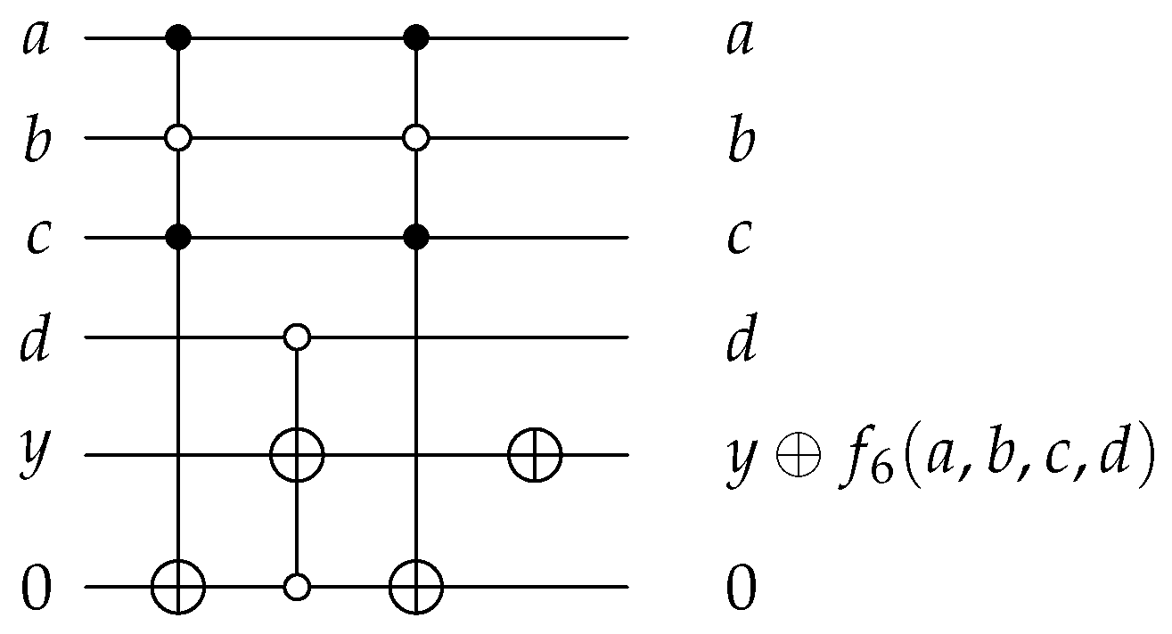
4.4.3. Grover’s Algorithm
Let f be a function . If and only if , then x is a solution. There are no restrictions regarding the number of solutions, ranging from 0 to M.
Let be the minimum number of bits needed to represent any possible input.
Let be a quantum oracle for at least qubits. The first m qubits encode the input, being the binary representation of x. The next qubit will be used to store . The rest of the qubits, if any, will be ancillary qubits needed to calculate f. Their number n depends on the way f has been implemented. This way of arranging the qubits may vary between implementations, sometimes using the last qubit as the output one, and the ones between it and the input qubits as the ancillary qubits. There are no reasons to prefer one to the other, neither of them affecting the result.
Let
be the quantum gate that implements the “Inversion About the Mean” operator. Its circuit can be seen in
Figure 10. This operator is applied once at the end of each Grover iteration. For the sake of efficiency, the
used at the last Grover iteration has one less gate, since it does not affect the results of the measurements that will be performed just after its application. It just affects the phase, which will be lost regardless. The circuit of this
gate is the one in
Figure 11. This gate cannot be used in any other iteration, for this phase change will affect the result otherwise.
The quantum circuit implementing Grover’s algorithm that we have used for these experiments can be seen in
Figure 12. The squared section may have to be repeated
times, with
g being the number of Grover iterations needed in this problem instance. If the right number of iterations are executed (depending on the number of solutions), there is a high chance that what we have measured is a solution. Any variation in the number of iterations or leaving garbage values in ancillary qubits can greatly decrease the odds of finding the answer. To obtain all possible solutions for the function
f, Grover’s algorithm may need to be executed multiple times. It is not exact like the previous two algorithms; it is probabilistic.
A different function has been defined for the specific number of qubits of each experiment, from 2 to 10. This number of qubits is not , but . Since we are trying to measure how the simulator performs, it would be unfair to make it depend on how well did we define the oracle. That is the reasoning behind this decision, to take into account the number of ancillary qubits. The logic functions we have defined are as follows:
;
;
;
;
;
;
;
;
.
The circuits that implement these functions can be found in
Appendix B. After calculating the number of Grover iterations, we will only need one per problem instance.
4.4.4. Results
Memory usage goes from exponential with dense vectors to linear with functional vectors, as shown in
Figure 13. What has been measured is the peak memory used. The exponential nature of the problem is not avoided by the first approach, having to store
complex numbers in memory. Meanwhile, when using functional matrices, the linear growth is due to the linearly increasing number of operations performed.
The lowest growth is that of the Deutsch–Jozsa algorithm execution, since each qubit only adds a measurement, that can be decomposed into multiplying by a projection matrix and by a scalar. We do not take into account the two extra Hadamard gates because of our functional matrix. The number of gates applied in the Bernstein–Vazirani algorithm ranges from 0 to n. On average, increasing the number of qubits by one will increase the number of operations by two, doubling the growth rate of the Deutsch–Jozsa algorithm execution. In spite of this, it is still linear. Finally, for Grover’s algorithm, the number of gates depends on the function to be implemented. Since we have tried to use the least possible number of qubits for each logic function, that means that adding one qubit increases the complexity of the oracle we have built. That is why it shows the highest memory usage of all algorithms.
Take into account that the memory specified in the rightmost graph will be used up on every computation node. It is not the sum of the memory used on each one. We have decided to show this because usually in supercomputing, you may have distributed memory instead of shared memory, so you are more interested in how much memory a node needs at most. To get the total memory used, multiply it by 16. It would still be linear.
As for the execution time in
Figure 14, it is shown to be growing exponentially as expected in both charts. The Bernstein–Vazirani algorithm is shown to be the slowest because of how we implemented the gate application functional matrix. It greatly benefits from the number of controls or anti-controls. Bernstein–Vazirani’s oracles are composed of gates with only one control, while Grover’s have a greater number of them.
The implementation for both the functional matrices and the full state vector simulator is available at Doki repository, QSimov’s simulation core, written in C.
https://github.com/Mowstyl/Doki/ (accessed on 1 June 2023).
The time needed to run the simulations is clearly lower when using full vectors rather than using functional ones. This is due to the fact that our functional matrix implementation repeats a lot of calculations, and shows that there is still room for improvement. Despite this difference, both approaches still have exponential asymptotic complexities.
These results show that algorithms that run over a universal quantum computer simulator can be executed with a very little amount of memory (with the same growth rate as the number of gates in the algorithm). They can also be easily parallelized to reduce their execution time with just a few messages between nodes ( messages per measurement). While functional matrices have been able to beat any other approach in terms of memory usage, lots of improvements and optimizations have to be made in order to be competitive in terms of execution time.
5. Conclusions and Further Work
Working with big-size matrices is a very common scenario when performing Quantum Computing Simulations. In the field of simulation using the circuit model, applying a gate is translated into a matrix product: the gate is represented by a matrix and the state of the system is represented by a column vector. Both of them grow exponentially which, therefore, drastically decreases the efficiency of the simulation.
In this paper, we make a proposal that reduces both the time and memory consumption of the stated problem using functional matrices that have been proven to outperform ordinary matrices to achieve a linear space complexity for quantum gates. In particular, a comparative study between the most commonly used mathematical structures and functional matrices has been performed. They have been tested under the scenarios and over the types of platforms that we understand to be the most representative.
When comparing these results to the ones achieved by simulators that directly apply the gates without calculating the tensor product, we find greater memory requirements but with smaller execution times, favoring the latter simulators. The exponentially growing nature of the matrices we are working with, along with the computational cost of the performed operations, leads to this result, making our first approach unable to match the speed of these simulators. This does not mean that functional matrices will never lead to better results than theirs. Since the development performed is just a proof of concept to test the capabilities of the functional matrices, the algorithms that implement matrix and tensor product used in this article are the naïve ones. Consequently, further work should search and implement algorithms with a smaller computational cost, leading to better results.
Apart from this, functional matrices can also be used to perform some hard calculus (in computational terms) as the partial trace of a system. This fact generates a general improvement in space complexity in any computation in which you could make use of them, for instance, whatever operation involving the density matrix calculated from the full-state vector.

 ,
, 


