Alzheimer’s Disease Prediction Using Deep Feature Extraction and Optimization

Abstract

Alzheimer’s disease (AD) is a prevalent neurodegenerative disorder that affects a substantial proportion of the population. The accurate and timely prediction of AD carries considerable importance in enhancing the diagnostic process and improved treatment. This study provides a thorough examination of AD prediction using the VGG19 deep learning model. The primary objective of this study is to investigate the effectiveness of feature fusion and optimization techniques in enhancing the accuracy of classification. The generation of a comprehensive feature map is achieved through the fusion of features that have been extracted from the fc7 and fc8 layers of VGG19. Several machine learning algorithms are employed to classify integrated features and recognize AD. The amalgamated feature map demonstrates a significant level of accuracy of 98% in the prognostication of AD, outperforming present cutting-edge methodologies. In this study, a methodology is utilized that makes use of the whale optimization algorithm (WoA), a metaheuristic approach to optimize features through feature selection. Feature optimization aims to eliminate redundant features and enhance the discriminatory power of the selected features. Following the optimization procedure, the F-KNN algorithm attained a precision level of 99%, surpassing the present state-of-the-art (SOTA) results reported in the current literature.

1. Introduction

Alzheimer’s disease (AD) is a neurodegenerative condition that gradually impairs cognitive functions, including memory, language and decision making. Early detection of AD is of paramount significance in the context of brain health. MRI is a significant diagnostic modality utilized for AD. The etiology of AD has been attributed to a combination of genetic, environmental and behavioral factors [1]. The formation of AD brains is attributed to the presence of two anomalous protein fragments: beta-amyloid and tau. The shape of anomalous protein fragments results in the creation of aggregates and filaments that impede intercellular communication within the brain, ultimately culminating in cellular demise and a subsequent decline in cognitive abilities [2,3]. AD is characterized by a range of symptoms, including memory impairment, alterations in mood and personality and challenges with orientation in time and place. These clinical manifestations are widely recognized as early indicators of the disease. As the condition develops, patients may face communication difficulties, appetite loss and more incredible difficulty with physical duties. AD may ultimately result in losing all cognitive and physical abilities and is often deadly. There is currently no cure for AD, and present therapies give only limited symptom alleviation [4]. Detection and treatment of the illness at an early stage are essential for optimizing life expectancy and improving the diagnostic system. Brain MRI scans are one of the most important diagnostic modality methods used to identify AD, and deep learning-based algorithms show robustness in enhancing the accuracy of these diagnoses. Ongoing research aims to uncover novel therapeutic targets and produce more effective AD therapies [5].

Artificial intelligence (AI) techniques are based on artificial neural networks (ANNs), deep learning (DL) and computer vision. The DL algorithms are meant to learn from massive datasets and may be used to generate predictions or judgments, depending on the data utilized for prognoses [6]. These algorithms learn more complex data features since they have several layers of connected blocks. These methods use several densely connected layers, unlike standard machine learning algorithms, which use one. Due to their ability to learn from complex data forms, including images, movies and spoken language, deep learning algorithms have been trending up in multiple domains [7]. The primary robust use of DL algorithms is their capacity to automatically extract relevant characteristics from incoming data without requiring human interaction. Deep learning algorithms have recently emerged as a potent tool for analyzing medical imaging data, such as brain MRI images. These algorithms can learn complicated visual cues that may be utilized to produce accurate illness status forecasts. Brain MRI-based Alzheimer’s disease prediction based on deep learning often comprises many stages [8]. During the first phase, preprocessing techniques are utilized in magnetic resonance imaging (MRI) images to mitigate noise and artifacts. In the next step, the preprocessed images are fed into a DL model that learns to detect the patterns and traits that distinguish healthy brains from AD brains [9]. Typically, the model’s training data comprises many MRI scans from healthy and AD-affected people. Once the model has been trained, it may be used to test MRI scans and predict the risk of Alzheimer’s disease. Typically, this is achieved by putting fresh MRI images into a model and generating a likelihood score for each scan. A higher probability score suggests Alzheimer’s disease is more likely [10,11].

Brain-based prediction includes evaluating MRI images of the brain to forecast a patient’s health or illness risk. Brain MRI is a noninvasive imaging method that offers comprehensive pictures of the brain’s anatomy and function [12]. Deep learning algorithms have shown potential for enhancing brain MRI-based predictions’ precision. These algorithms can learn and utilize complicated visual cues to forecast a patient’s health condition and illness risk, particularly for patients with neurological diseases for whom treatment results could be predicted through machine learning techniques [13]. By studying changes in the structure and function of the brain over time, these algorithms can anticipate how a patient will react to various therapies, enabling physicians to personalize treatment for each patient. Using brain MRI and deep learning to predict AD has shown encouraging results in many studies [14]. In recent research published in the Journal of Alzheimer’s Disease, a deep learning system trained on MRI scans predicted AD with a 95 percent accuracy rate. Brain MRI-based, deep learning-based AD prediction can enhance the early identification and treatment of disease, leading to improved patient outcomes. However, further study is necessary to evaluate the accuracy and dependability of these algorithms in clinical contexts [15]. To address the challenges presented in AD prediction, a deep CNN model-based prediction model has been proposed with the following traits:

• Transfer learning is employed on VGG19 with fine-tuned hyperparameters for deep feature extraction from the fc7 and fc8 layers.
• The process of feature concatenation is performed to create a unified feature space by considering the highest value.
• Redundancy in the features is eliminated using an updated version of the WoA with optimal settings.

The subsequent sections of this document are arranged in the following manner. Section 2 contains a presentation of the related work. Section 3 outlines the proposed approach, which involves optimizing features, fusing them and using ML classifiers for classification. Section 4 of this paper presents the results, while Section 5 provides the conclusion.

2. Related Work

The investigation of AD diagnosis using brain MRI and deep learning techniques has garnered growing attention in computer-aided diagnostics [16,17]. Deep neural networks offer considerable potential for identifying brain illnesses and providing prognosis predictions based on neuroimaging data, but significant, labeled training datasets are often needed for excellent predictive accuracy [15,18]. The authors of [19] explored a variety of pretraining and transfer learning (TL) [20] techniques to construct usable MRI representations for downstream tasks that lack significant quantities of training data, such as AD classification [21], in the absence of vast amounts of training data. The scientists studied 4098 3D T1-weighted brain MRI images from the Alzheimer’s Disease Neuroimaging Initiative (ADNI) cohort and 600 scans from the Open Access Series of Imaging Studies (OASIS3) [22] cohort to assess the suggested pretraining methodologies for identifying AD. The authors first trained three-dimensional and two-dimensional convolutional neural network (CNN) architectures. The authors examined combinations of several pretraining procedures based on (1) supervised, (2) contrastive and (3) self-supervised learning, employing pretraining data from inside and beyond the MRI domain. In these studies, the 3D CNN pretrained with contrastive learning produced the best overall results on T1-weighted scans for AD classification and exceeded the baseline by 2.8% when trained using all the ADNI training data. The authors also proved the validation performance as a function of the training dataset size and pretraining technique. TL provided considerable advantages in low-data environments, resulting in a 7.7% improvement in performance. A uniform manifold approximation (UMAP) projection of the high-dimensional model embedding space revealed a better clustering of test participants’ diagnostic groups when the pretrained DL model was employed for AD classification. In addition, saliency maps showed the extra brain scan activation areas that contributed the most to the final prediction score based on pretraining. This study built a DL-based pipeline for accurate AD diagnosis and stage classification. The suggested analytic pipeline employed shallow CNN architecture for MRI, 2D T1-weighted brain scans. The proposed pipeline includes a rapid and accurate AD diagnostic module, a global classification (average versus mild cognitive impairment (MCI) versus AD) and a local classification. As the prodromal stage of Alzheimer’s disease, it is much more challenging to classify MCI into mild dementia (MD), very mild dementia (VMD) and moderate dementia (MoD). In addition, the authors compared their methodology to advanced DL architectures, such as DenseNet121, ResNet50 [23], VGG16 [24], EfficientNetB7 [25] and InceptionV3 [26]. The presented findings demonstrated the robustness and high accuracy of the recommended procedure. Using T1-weighted magnetic resonance imaging (MRI) images, the authors of [27] evaluated the effectiveness of a CNN algorithm to distinguish temporal lobe epilepsy (TLE) versus patients with Alzheimer’s disease against healthy controls. The authors utilized feature visualization tools to discover the areas CNN uses to determine illness types. It was shown that AI (CNN deep learning) can categorize and differentiate TLE, highlighting its potential value for future computer-assisted radiological examinations of epilepsy, particularly for individuals who do not present immediately recognizable TLE-associated MRI characteristics.

Using MRI images, the authors of [28] classified Alzheimer’s disease using deep learning algorithms. Compared with conventional machine learning approaches, the accuracy of AD prediction using DL algorithms was much higher. Using MRI images, the authors [29] predicted the progression of MCI to AD using a deep learning system. The research indicated that the deep learning system predicted the onset of AD within three years with an accuracy of 83.3 percent. MRI images were combined with deep learning algorithms to diagnose AD. The research in [30] showed that deep learning algorithms accurately diagnose Alzheimer’s disease, reaching more than 95% accuracy in some studies. The authors used the DL algorithm to classify AD with T1-1-weighted, T2-weighted, and diffusion-weighted images. According to the study carried out in [31], which also included diffusion-weighted images, the DL method correctly detected AD at a rate of 92.3 percent. The DL system was used to diagnose AD and predict prognoses using neuroimaging techniques with magnetic resonance imaging (MRI), positron emission tomography (PET) and cerebrospinal fluid (CSF) biomarkers which, according to the study, showed excellent diagnostic and predictive accuracy. According to [32], a deep learning system can improve brain MRI-based Alzheimer’s disease prognosis, with some studies reaching an accuracy of 90%. More studies are needed to confirm these results in different populations [33]. The summary of the detailed model is discussed in the Related Work section with the dataset being used and accuracy presented in

Table 1. Comparison of existing studies discussed in literature.

Ref.	Year	Dataset	Model	Accuracy
[6]	2022	MRI Brain Images	DL model	96%
[7]	2022	MRI	Deep TL model	93.52%
[10]	2023	MRI Images	DL-based radiomics	93.50%
[18]	2022	MRI, PET	AD dataset	94.61%
[19]	2023	MRI	Deep CNN	89%
[20]	2023	Brain Dataset	AlexNet framework	98.35%
[22]	2023	MRI	CNN	98.67%
[23]	2022	MRI	ML	94.64%
[24]	2022	MRI	DL and ML	91.70%
[25]	2022	MRI	ML	95.30%
[26]	2022	MRI	DL	82.2%

.

3. Materials and Methods

The present study introduces a new approach for predicting AD by utilizing the VGG19 architecture, feature fusion and optimization techniques. The methodology entails the extraction of features from the fc7 and fc8 layers of VGG19, followed by their fusion to generate a comprehensive feature map. Furthermore, this study utilizes a feature optimization methodology utilizing the whale optimization algorithm (WoA) to augment the discriminatory capabilities of the features. Subsequently, several ML algorithms are employed for classification purposes. The architecture of the proposed method is shown in Figure 1.

3.1. Dataset

The Alzheimer’s Disease Neuroimaging Initiative (ADNI) [34] is a collaborative effort that integrates resources and knowledge from both the private and public sectors to investigate individuals afflicted with AD. The researchers associated with the Alzheimer’s Disease Neuroimaging Initiative (ADNI) collect, validate, and utilize diverse types of data, including MRI and positron emission tomography (PET) scans, genetic data, cognitive evaluations, cerebrospinal fluid (CSF) and blood biomarkers to potentially identify factors that can predict the onset of the disease. The dataset utilized to validate the performance of the proposed method was extracted from the ADNI and is accessible publicly on the Kaggle [35] platform. The dataset was composed of three distinct categories, specifically AD, individuals with normal cognitive function (CN) and those experiencing cognitive impairment (CI). The number of images per class was an AD class comprising 1124 images, a CI class with 2590 images and a CN class with 1440 images. The class imbalance was handled using gat augmentation. The data augmentation process was employed to increase the samples per class as well as address the class imbalance problem. During the augmentation rotation, flipping, mirroring, and scaling were performed.

3.2. Deep Feature Extraction

Deep learning has been employed extensively recently in several tasks [36] involving disease detection and prediction [15,37]. The VGG-19 [38] model was proposed as a solution to tackle the problem of vanishing gradients that arise in deep convolutional neural networks. It is widely acknowledged that deep neural networks possess a considerable quantity of parameters, which endows them with the capability to acquire intricate patterns and depictions from their source data. The process of training deep networks poses a significant challenge due to the occurrence of the vanishing gradient problem. This problem occurs when the gradients diminish significantly as they backpropagate through the layers. This issue poses a challenge to the network’s ability to learn with optimal efficacy. In our proposed method, we utilize VGG19 for feature engineering.

VGG-19 is a 19-layer-deep neural network comprising 16 convolutional layers and 3 fully connected (FC) layers. It was designed to classify images using the ImageNet dataset [39], which consists of over 1 million images belonging to a thousand classes. The convolutional layers of VGG19 use 3 × 3 filters with a 1-pixel stride, followed by max pooling layers with a 2 × 2 window size and a 2-pixel stride. This design and architecture of the network can classify more complex image data. Convolutional and fully linked layers of VGG19 use the rectified linear unit (ReLU) activation function [40]. The convolution operation over a location $(x,y)$ with a filter $L$ having a size $M\times M$ for an input feature space $I$ with dimensions $W\times H$ can be defined as follows:

$$O(x,y)=\sum _{i=1}^M\sum _{j=1}^{M}I\left(x+i-1,y+j-1\right)\times L(i,j)$$

(1)

where the output at location $(x,y)$ is presented as $O(x,y)$. The filter used in the convolution operation is denoted by $L$. The ReLU function is often employed in deep learning models due to its computational efficiency and has shown effectiveness in practice [4]. VGG19 utilizes convolutional layers with ReLU activation functions and max pooling layers to extract features and reduce spatial dimensions. ReLU activation functions are also used by the final, fully interconnected network layers. The activation function of ReLU applied to FC layers for feature extraction can be defined over an input $x$ as

$$ReLU\left(x\right)=max(0,x)$$

(2)

The initial fully connected layer computes a total of 4096 × 25 learnable weights and 4096 × 1 bias. The implementation of a dropout layer between fully connected layers has been observed to mitigate the 50% dropout rate. The final layer contains a total of 1000 by 4096 learnable weights. The feature map resulting from activation has dimensions of 1 × 1 × 1000 at the FC7 layer and 1 × 1 × 4096 at the FC8 layer. The VGG19 architecture for feature engineering is shown in Figure 2.

3.3. Feature Concatenation

The process of feature concatenation involves the incorporation of two feature spaces into a unified vector through a novel equation that accentuates the highest value. Although it improves accuracy, it also results in elevated prediction and training durations. The composite vector, represented by $Y_3$, is characterized as the highest value derived from $Y_1\in {FV}_1$ and $Y_2\in {FV}_2$ while guaranteeing that $Y_3$ is devoid of any duplicated elements. The pseudo code of the feature concatenation is presented below in Algorithm 1. The feature vector $Y_3$ is a composite entity with dimensions of ${FV}_1\times 4096$ and ${FV}_2\times 1000$. The concatenated feature map will be as follows

$$\widetilde{Y_3}=Y_3\leftarrow Maximum\left(Y_1,Y_2\right)\&Y_3\in NotRepeated$$

(3)

Algorithm 1: Pseudo code of feature concatenation

Normalize ($Y_1$) Normalize ($Y_2$) if length ($Y_1$) < length ($Y_2$): Extend $Y_1$ to match the length of $Y_2$ else: Extend $Y_2$ to match the length of $Y_1$ $Y_3$= empty_vector of length ($Y_1$) used_features = empty_set for i from 0 to length ($Y_1$) − 1: weighted_$Y_1$_value = $W_1$ * $Y_1$[i] weighted_$Y_2$_value = $W_2$ * $Y_2$[i] if weighted_$Y_1$_value > weighted_$Y_2$_value and $Y_1$[i] no longer in used_features: $Y_3$[i] = $Y_1$[i] else if weighted_Y_2_value >= weighted_$Y_1$_value and $Y_2$[i] no longer in used_features: $Y_3$[i] = $Y_2$[i] else: $Y_3$[i] = some_fallback_logic () used_features.Upload ($Y_3$[i])

3.4. Feature Optimization

The implementation of feature optimization methodologies enhances the efficacy of machine algorithms by eliminating extraneous and duplicative features. Various algorithms are employed in disease detection to enhance data optimization for improved disease diagnosis. Our proposed methodology for AD prediction involves utilization of the whale optimization algorithm (WOA) to optimize features. The feature selection algorithm (WOA) was applied to a fused feature map, resulting in a feature map with reduced dimensionality and eliminated feature redundancy [41].

Whale Optimization Algorithm

The whale optimization algorithm (WOA) [41] was employed for feature optimization to minimize the presence of redundant and irrelevant features. The process of optimization involves a dual-step approach. Initially, the spiral position is revised, subsequently resulting in the encirclement of the prey. During the second stage, a randomized search is conducted to locate the prey.

Regarding encircling prey, whales employ a strategy of locating their prey and encircling it. The precise whereabouts of the prey within the search area remains unknown. Assuming that the dominant species is the most advantageous prey, the existing search agents endeavor to attain optimality by altering their spatial position. The presentation showcases the search agents’ behaviors:

$$\overrightarrow{Z}\left(v+1\right)=\overrightarrow{Z^{*}}\left(u\right)-\overrightarrow{A}·\overrightarrow{F},$$

(4)

$$\overrightarrow{F}=\left|\overrightarrow{D}·\overrightarrow{Z^{*}}\left(u\right)-\overrightarrow{Z}(u)\right|,$$

(5)

The notation $\overrightarrow{Z^{*}}\left(u\right)$ denotes the optimal location of the whale after iteration u. The present coordinates of the whale are denoted by the vector $\overrightarrow{Z}\left(u+1\right)$, while the magnitude of the distance between the whale and its prey is represented by the vector $\overrightarrow{F}$, with the double vertical bars indicating the absolute value. The vectors $\overrightarrow{A}$ and $\overrightarrow{D}$ are computed as coefficient vectors:

$$\overrightarrow{A}=2·\overrightarrow{a}·\overrightarrow{s}+\overrightarrow{a}$$

(6)

$$\overrightarrow{D}=2·\overrightarrow{s}$$

(7)

The magnitude of a vector can be reduced by contraction, leading to transformation of the amplitude of the vector $\overrightarrow{A}$ into vector a through iterative processes. The variable $\overrightarrow{A}$ is defined as a range of values (−a, a) between negative and positive a, while the variable A undergoes a decremental change from 2 to 0 iterations. The optimal agent location and initial agent location are established by randomly selecting a value for the vector $\overrightarrow{A}$ within the range of $(-1,1)$.

For spiral position updating, the process of helix formation in whales for prey tracking involves computation of the spatial separation between the location of the whale $\left(Z,Q\right)$ and that of the prey $\left(Z^{*},Q\right)$. The act of advancing towards prey is commonly expressed as follows:

$$\overrightarrow{Z}\left(u+1\right)=e^{bk}·\cos \left(2\pi k\right)·\overrightarrow{F^{*}}+\overrightarrow{F^{*}}(u)$$

(8)

$$\overrightarrow{F^{*}}=\left|\overrightarrow{Z^{*}}\left(u\right)-Z(u)\right|$$

(9)

The logarithmic spiral’s configuration is determined by a consistent parameter, denoted as $k,$ and a stochastic variable that spans the interval [−1, 1]. The whales’ ability to perform reduction while changing their location is facilitated by their spiral movement. The probability of being chosen is equally distributed at 50% for both the spiral and diminishing encircling methods:

$$\overrightarrow{Z}\left(u+1\right)=\left\{\begin{array}{c}\overrightarrow{Z^{*}}-\overrightarrow{A}·\overrightarrow{F},ifp<0.5,\\ e^{bk}·\cos \left(2\pi k\right)·\overrightarrow{F^{*}}+\overrightarrow{Z^{*}}\left(u\right),ifp\ge 0.5,\end{array}\right.$$

(10)

The variable $p$ is a uniformly distributed random number that takes values between 0 and 1.

For prey searching, the initial phase of hunting for prey is commonly referred to as the exploration process and is contingent upon the fluctuations of vector $\overrightarrow{A}$. Whales engage in stochastic foraging behavior, whereby they conduct non-directed searches to locate prey based on its spatial distribution. The presence of whales in each area causes search agents to avoid conducting searches in that location. The WOA algorithm employs a vector $\overrightarrow{A}$ comprising randomly generated values that fall within the range from negative one to positive one. During the exploration phase, the selection of the search agent is randomized. The utilization of random selection endows the WOA algorithm with global search capabilities, thereby mitigating the issue of local optimization. The global search feature is presented in the interface:

$$\overrightarrow{Z}\left(u+1\right)=\overrightarrow{Z_{rand}}-\overrightarrow{A}·\overrightarrow{F},$$

(11)

$$\overrightarrow{F}=\left|\overrightarrow{C}·\overrightarrow{Z_{rand}}-\overrightarrow{Z}\right|$$

(12)

The symbol $\overrightarrow{Z_{rand}}$ denotes a randomly selected whale from the specified population.

The WOA commences by assigning arbitrary values to the whale population, assuming the optimal solution of the function with either the minimum or maximum value. The pseudo code of the fine-tuned and improved WoA is presented below in Algorithm 2.

Algorithm 2: Pseudo code of the whale optimization algorithm

Pseudocode of whale optimization algorithm Step 1: Initialization (Whale population) $Z_i$ where $(i=\mathrm{1,2},3,\dots \dots n)$ Step 2: The computation of fitness for every solution. $Z^{*}=$ best search agent Step 3:   While $(u<Max\_iteration)$         For every solution             Updated $c,A,C,M$ and $p$                If1 $(p<0.5)$                    If2 $(/A/<1)$ Revise the present location of the search agent by Equation (1).                    Else if2$(/A/>1)$ The process of selecting a random search agent. ${(Z}_{rand})$ The location of the search agent is subject to modification based on Equation (7).                    End if2                Else if1$(p\ge 0.5)$ The location of the search agent is subject to modification by Equation (5).                    End if1        End for Examine the trajectory of a search agent if it deviates from its designated search location and alters its course. Change $Z^{*}$ if the better solution is presented $u=u+1$        End While Step 4: Return $Z^{*}$

4. Results

The method for recognizing AD that has been proposed was implemented on a dataset available publicly on Kaggle. The dataset consists of various types of MRI scans exhibiting a variety of orientations. The method employed for training and testing involved the utilization of a 70:30 approach. The process of simulating the proposed method was executed on a desktop computer featuring an Intel i7 8th generation central processing unit, 16 gigabytes of random access memory and an 8-gigabyte graphics processing unit. Various classifiers were utilized to classify AD diseases, and those that demonstrated greater accuracy were chosen as robust classifiers. The efficacy of the applied technique was assessed through diverse performance evaluation metrics such as precision, recall, F1 score, false negative rate (FNR) and computational duration.

4.1. AD Prediction Results of Features Extracted from fc7

The models’ performance was assessed using several measures, including accuracy, precision, recall, F1 score, false negative rate (FNR) and time (in seconds), and they made use of extracted features from the VGG 19 fc7 layer. The study employed several models, each with its respective performance metrics evaluation. The models included W-KNN, F-KNN, ES-KNN [42], C-SVM, Q-SVM and MG-SVM [43].

Table 2. Alzheimer’s disease prediction using extracted features from VGG 19 fc7 layer.

Method	Accuracy (%)	Precision (%)	Recall (%)	F1 Score (%)	FNR (%)	Time (s)
F-KNN	97.3	95.4	96.8	96.1	2.7	900
C-SVM	96.4	93.1	95.6	94.3	3.6	712
Q-SVM	94.2	91.2	94.3	92.7	5.8	656
MG-SVM	91.8	92	91.6	91.6	8.2	989
W-KNN	92.3	92.3	92.6	92.3	7.7	1256
ES-KNN	97.1	97.3	96.3	96.3	2.9	1522
ESD	93.9	94	94	93.66	6.1	1823

displays the accuracy, precision, recall and F1 score for each model, which are frequently used measures for assessing the effectiveness of machine learning models. Also included is the false negative rate (FNR), which is the proportion of real Alzheimer’s patients that were mistakenly labeled as non-Alzheimer’s cases.

The F-KNN and ES-KNN models demonstrated superior performance in predicting AD when using the derived features of the VGG 19 fc7 layer. These models, with accuracy levels of 97.3% and 97.1%, respectively, had the highest accuracy values. Furthermore, these models had the lowest false negative rates (FNRs) of any model, with F-KNN having an FNR of 2.7% and ES-KNN having an FNR of 2.9%. In addition, F-KNN and ES-KNN both showed reasonably quick prediction times when compared with the other models, taking 900 and 1522 s, respectively.

The MG-SVM model, on the other hand, performed the poorest in terms of accuracy, obtaining only 91.8% accuracy. Additionally, this model had the highest FNR of 8.2%, indicating a significant rate of incorrectly identifying real Alzheimer’s cases as non-Alzheimer’s cases. Additionally, this model’s forecast time, which was 989 s, was rather long. The best-performing classifier’s (F-KNN) performance was also evaluated using the confusion matrix and ROC curve presented in Figure 3.

Table 3. Proposed model performance evaluation measures per class using fc7 layer features.

Classes	Accuracy (%)	Precision (%)	Recall (%)	F1 Score (%)
AD	98.31	98.31	98.31	98.31
CI	97.71	97.71	97.71	97.71
CN	98.56	98.56	98.56	98.56

displays the performance evaluation metrics for a suggested model for categorizing Alzheimer’s, assessed by class. The highest accuracy was achieved in the CN class with 98.56%, and the lowest accuracy was achieved in the CI class with 97.71%.

4.2. AD Prediction Results of Features Extracted from fc8

Table 4. Alzheimer’s disease prediction using extracted features from the fc8 layer.

Method	Accuracy (%)	Precision (%)	Recall (%)	F1 Score (%)	FNR (%)	Time (s)
F-KNN	96.2	96	96	96.33	3.8	900
C-SVM	95.5	95.6	95.4	95.6	4.5	712
Q-SVM	91.7	91.6	92	92	8.3	809.35
MG-SVM	88.5	88.3	88.3	88.6	11.5	840.25
W-KNN	91.2	91.3	91.66	91	8.8	1182.7
ES-KNN	95.5	95.6	95.6	95.6	4.5	2167.9
ESD	88.4	88	88.6	88.33	11.6	18,446

shows that, with accuracy values ranging from 95.5% to 96.2%, F-KNN, C-SVM and ES-KNN outperformed the other algorithms in terms of accuracy, precision, recall and F1 score. While the accuracy of Q-SVM, MG-SVM, W-KNN and ESD ranged from 88.4% to 91.7%, they were less accurate. The FNR shows the proportion of instances belonging to a class that was mistakenly categorized as not being a member of that class. A higher FNR denotes more false negatives, or occurrences that should belong to a class but are incorrectly labeled as not being part of it. The table shows that the algorithms with the greatest FNRs were MG-SVM and ESD, which shows that they were less accurate in accurately classifying instances that belonged to a class. The amount of time needed by each method to complete the classification task differed greatly, ranging from 900 s (F-KNN) to 18,446 s (ESD).

The required tradeoff between classification performance and computing economy thus determines the selection of an optimal method. The performance of the robust method with the highest accuracy was also validated with the confusion matrix and ROC curve in Figure 4.

In

Table 5. Proposed model performance evaluation measures per class using fc8 layer features.

Classes	Accuracy (%)	Precision (%)	Recall (%)	F1 Score (%)
AD	98.09	98.09	98.09	98.09
CI	96.48	96.48	96.48	96.48
CN	97.88	97.88	97.88	97.88

, for all three classes, the suggested model obtained excellent levels for accuracy, precision, recall and F1_score, with the AD class recording the highest values. For the AD class, the model obtained 98.09% accuracy, 98.09% precision, 98.09% recall and 98.09% for the F1 score. The model’s accuracy for the CI and CN classes was 96.48% and 97.88%, respectively, with matching values for precision and recall and F1 scores of 96.48% and 97.88%, respectively.

4.3. AD Prediction Results of Feature Fusion Extracted from fc7 and fc8

In terms of accuracy, precision, recall, F1 score, FNR and time,

Table 6. AD prediction using feature concatenation.

Method	Accuracy (%)	Precision (%)	Recall (%)	F1 Score (%)	FNR (%)	Time (s)
F-KNN	98	97	98.3	97.6	2	972
C-SVM	98	97.6	98.3	98	2	912.2
Q-SVM	96.4	96.3	96.3	96.3	3.6	879
MG-SVM	94.4	94.3	94.6	94.3	5.6	1420.5
W-KNN	92.4	92.3	92.6	92.3	7.6	1882.7
ES-KNN	97.5	97.3	97.3	97.6	2.5	2667.9
ESD	95.7	95.6	96	95.6	4.3	3752.2

shows the performance evaluation metrics for various approaches using feature fusion extracted from fc7 and fc8. The F-KNN and C-SVM algorithms both scored 98%, which was the highest accuracy rating. The accuracy ratings for the Q-SVM and MG-SVM approaches were lower, coming in at 96.4% and 94.4%, respectively. The even less accurate approaches, namely W-KNN and ESD, scored 92.4% and 95.7%, respectively.

The ESD approach was the slowest, taking 3752.2 s to finish, while the F-KNN method was the fastest in terms of time, finishing in just 972 s. Overall, the F-KNN approach was the quickest, and the C-SVM method was the most accurate.

Table 7. Proposed model performance evaluation measures per class using feature fusion.

Classes	Accuracy (%)	Precision (%)	Recall (%)	F1 Score (%)
AD	98.64	98.64	98.64	98.64
CI	98.31	98.31	98.31	98.31
CN	98.98	98.98	98.98	98.98

exhibits the performance evaluation metrics for each class in a classification task, where the classes are denoted by AD, CI and CN. The assessment metrics used were accuracy, precision, recall and F1 score, which were quantified as percentages.

Upon examination of the accuracy metrics, it is evident that the model demonstrated exceptional performance across all three categories, attaining a precision rate of 98.64% for the AD class, 98.31% for the CI class and 98.98% for the CN class. The results indicate that the model achieved accurate classification rates of 98.64%, 98.31% and 98.98% for the AD, CI and CN samples, respectively. The performance of the highest-performing ML classifier was also evaluated using the ROC curve and the confusion matrix in Figure 5.

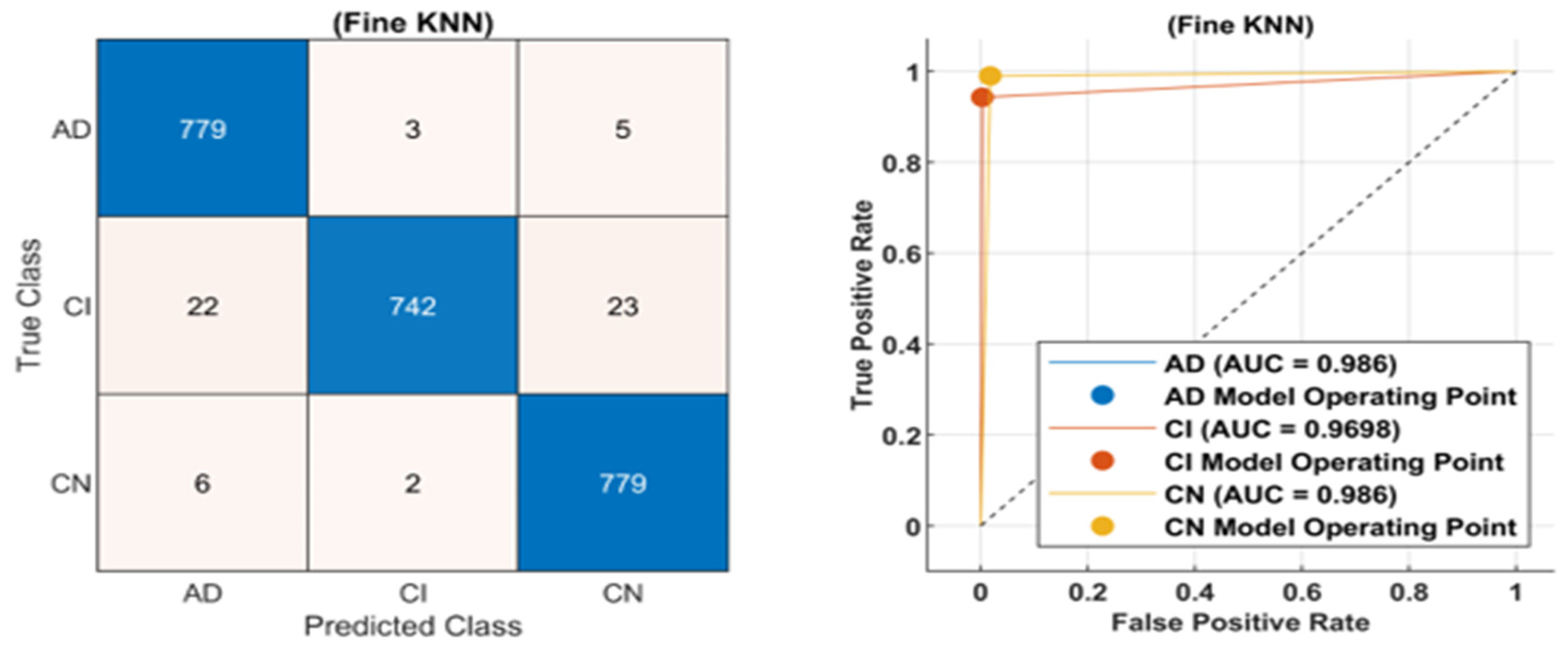
4.4. AD Prediction Results of Feature Optimization

In

Table 8. Results of the proposed method using feature optimization.

Method	Accuracy (%)	Precision (%)	Recall (%)	F1 Score (%)	FNR (%)	Time (s)
F-KNN	99	99.6	99.6	99.6	1	12
C-SVM	97.5	98	98	98	2.5	39.15
Q-SVM	95.3	95.3	95.3	95	4.7	54.42
MG-SVM	94	94.3	94.3	94	6	61.52
W-KNN	92	92	92.3	91.66	8	65.35
ES-KNN	92.4	92.6	92.3	92.3	7.6	89.65
ESD	97.3	97.3	97.3	97	2.7	109.35

, the AD prediction results are presented using a feature optimization approach which resulted in a higher prediction rate as well as a decrease in the computational cost. The F-KNN method exhibited the highest level of precision, attaining a 99% accuracy rate. The results demonstrate that F-KNN achieved a classification accuracy of 99%, thereby establishing it as the most precise approach among the enumerated methods. W-KNN, which had an accuracy of 92%, had the lowest accuracy of any approach. The findings suggest that W-KNN exhibited a comparatively inferior classification accuracy with alternative methodologies, accurately classifying only 92% of the instances. F-KNN exhibited the shortest computational duration, accomplishing the task within 12 s. Conversely, the computation time for ESD was the lengthiest, amounting to 109.35 s. A trade-off appeared to exist between the accuracy and computation time. The F-KNN method exhibited superior accuracy and computational efficiency compared with the W-KNN method, which demonstrated lower accuracy and a higher computational time. This implies that F-KNN could potentially offer superior efficiency in terms of both precision and computational cost.

The method put forth was compared to pre-existing methods for the identification of AD and demonstrated comparable levels of accuracy and computational efficiency. A comprehensive comparison and analysis of the proposed method with the existing methodologies has been presented.

Lu et al. [44] proposed a multimodal multi-scale deep CNN approach for the prediction of AD disease and achieved an accuracy of 82.4%. A DL- and ensemble learning-based model [45] has been proposed for the early stage diagnosis of AD with an overall accuracy of 97.65%. In [46], a robust AD classification method was presented. The presented technique used deep CNN and mobility data for timely diagnosis of the stage of AD in patients. Kundaram et al. [47] came up with a deep CNN-based method that accurately classifies AD, normal control (NC), and mild cognitive impairment (MCI) on the ADNI dataset. Nguyen et al. [7] presented an ensemble learning-based approach for AD prediction by combining traditional ML and DL approaches and achieving an accuracy of 96%. Sisodia et al. [48] came up with a DL-based technique to identify the different stages of AD and attained an accuracy of 93.52%. In [12], segmentation was employed with deep learning for the accurate prediction of AD, with an accuracy of 93.50%. The authors of [48] employed DL approaches to determine AD using the disease ontology method and accurately predicted AD with an accuracy of 94.61%. Shamrat et al. [28] proposed an Alzheimer Net to predict AD robustly using DL approaches, with an accuracy of 98.67%. The proposed DL-based method demonstrated superior performance compared with the state-of-the-art (SOTA) methodologies presented in

Table 9. Proposed method comparison with SOTA.

Reference	Year	Method	Accuracy
[44]	2018	Deep CNN	82.4%
[45]	2019	ConvNets	97.65%
[46]	2020	Deep CNN	91%
[47]	2021	Deep CNN	98.57%
[7]	2022	Ensemble of ML and DL	96%
[12]	2022	Segmentation and DL	93.50%
[49]	2022	DL-based ontology	94.61%
[48]	2023	Deep CNN	93.52%
[28]	2023	DL-based Alzheimer Net	98.67%
Proposed		DL and Feature Optimization	99%

.

5. Discussion

The strategy proposed for predicting AD involves employing several machine learning models and feature extraction utilizing a fine-tuned VGG19 model. The effectiveness of the proposed AD prediction approach was assessed using a publicly accessible dataset sourced from Kaggle. This dataset was obtained from the ADNI and contains MRI images captured from various angles. The proposed approach includes dividing the dataset into training and testing sets at a ratio of 70:30. This division was used to evaluate the performance of the model. The study findings indicate that the F-KNN and ES-KNN models exhibited superior performance when utilizing features extracted from the VGG 19 fc7 layer. These models achieved accuracy levels of 97.3% and 97.1%, respectively. The models exhibited a low incidence of false negatives (FNs) and reasonable prediction times. The accuracy of Q-SVM, MG-SVM, W-KNN, and ESD for AD prediction utilizing the fc8 layer features varied from 88.4% to 91.7%; in other words, they were less accurate. The FNR displays the percentage of instances that should belong to a class but are incorrectly identified as not belonging to that class. A higher rate of false negatives, which refers to instances that should be categorized as belonging to a particular class but are incorrectly labeled as not belonging, results in an increased FNR.

Additionally, the proposed technique was evaluated by utilizing features extracted from the fc7 and fc8 layers and featured concatenation of both layers. The model performance was evaluated based on accuracy, precision, recall and computation time. Feature fusion enhanced accuracy by compromising the computational cost. After analyzing the accuracy metrics, it was apparent that the model exhibited outstanding performance in each of the three categories after feature fusion. Specifically, it achieved a precision rate of 98.64% for the AD class, 98.31% for the CI class and 98.98% for the CN class. The findings suggest that the model demonstrated high levels of accuracy in classifying the AD, CI and CN samples, with rates of 98.64%, 98.31% and 98.98%, respectively. To address the computation cost issue, feature reduction was performed to eliminate the redundant features and select the most prominent features. The feature optimization proved robust in terms of the reduction in computational cost and increase in accuracy. The proposed model attained remarkable precision and accuracy levels for each of the categories (AD, CI and CN) and surpassed other contemporary methods in terms of both accuracy and computational efficiency. This study offers a thorough assessment and contrast of various models and techniques for feature extraction in predicting AD. It emphasizes the significance of selecting suitable models and feature layers to attain precise and efficient outcomes.

6. Conclusions

The proposed technique provides a thorough investigation into the prediction of AD utilizing the VGG19 framework, feature fusion and optimization methodologies. The findings indicate that the suggested approach is effective in improving the precision of classification. Initially, a high level of accuracy of 98% was attained through the fusion of characteristics derived from the fc7 and fc8 layers of VGG19. Moreover, the utilization of the WoA in feature optimization resulted in a noteworthy enhancement, achieving a remarkable precision of 99% in predicting AD, exceeding the current leading outcomes. The results underscore the possibility of enhancing the precision of AD prediction through the utilization of deep learning architectures, feature fusion and optimization methods. The methodology put forth in this study makes a significant contribution to the field of AD research and offers valuable insights for the timely diagnosis and efficacious treatment of this condition. Subsequent investigations may expand upon these results by examining alternative architectures, exploring diverse feature selection methods, and incorporating multimodal data to enhance the predictive capabilities of Alzheimer’s disease.

References

1. Marwa, E.-G.; Moustafa, H.E.-D.; Khalifa, F.; Khater, H.; AbdElhalim, E. An MRI-based deep learning approach for accurate detection of Alzheimer’s disease. Alex. Eng. J. 2023, 63, 211–221. [Google Scholar]
2. DeTure, M.A.; Dickson, D.W. The neuropathological diagnosis of Alzheimer’s disease. Mol. Neurodegener. 2019, 14, 1–18. [Google Scholar]
3. Chen, H.; Qiao, H.; Zhu, F.; Chen, L. Alzheimer’s Disease Clinical Scores Prediction based on the Label Distribution Learning using Brain Structural MRI. In Proceedings of the 2022 International Joint Conference on Neural Networks (IJCNN), Padua, Italy, 18–23 July 2022; pp. 1–8. [Google Scholar]
4. Lu, B.; Li, H.-X.; Chang, Z.-K.; Li, L.; Chen, N.-X.; Zhu, Z.-C.; Zhou, H.-X.; Li, X.-Y.; Wang, Y.-W.; Cui, S.-X. A practical Alzheimer’s disease classifier via brain imaging-based deep learning on 85,721 samples. J. Big Data 2022, 9, 1–22. [Google Scholar]
5. Sudar, K.M.; Nagaraj, P.; Nithisaa, S.; Aishwarya, R.; Aakash, M.; Lakshmi, S.I. Alzheimer’s Disease Analysis using Explainable Artificial Intelligence (XAI). In Proceedings of the 2022 International Conference on Sustainable Computing and Data Communication Systems (ICSCDS), Erode, India, 7–9 April 2022; pp. 419–423. [Google Scholar]
6. Liu, S.; Masurkar, A.V.; Rusinek, H.; Chen, J.; Zhang, B.; Zhu, W.; Fernandez-Granda, C.; Razavian, N. Generalizable deep learning model for early Alzheimer’s disease detection from structural MRIs. Sci. Rep. 2022, 12, 17106. [Google Scholar] [PubMed]
7. Nguyen, D.; Nguyen, H.; Ong, H.; Le, H.; Ha, H.; Duc, N.T.; Ngo, H.T. Ensemble learning using traditional machine learning and deep neural network for diagnosis of Alzheimer’s disease. IBRO Neurosci. Rep. 2022, 13, 255–263. [Google Scholar] [PubMed]
8. Payton, E.; Khubchandani, J.; Thompson, A.; Price, J.H. Parents’ expectations of high schools in firearm violence prevention. J. Community Health 2017, 42, 1118–1126. [Google Scholar]
9. Ullah, Z.; Jamjoom, M. A Deep Learning for Alzheimer’s Stages Detection Using Brain Images. Comput. Mater. Contin. 2023, 74, 1457–1473. [Google Scholar] [CrossRef]
10. Thangavel, P.; Natarajan, Y.; Preethaa, K.S. EAD-DNN: Early Alzheimer’s disease prediction using deep neural networks. Biomed. Signal Process. Control 2023, 86, 105215. [Google Scholar] [CrossRef]
11. Khatri, U.; Kwon, G.-R. Alzheimer’s disease diagnosis and biomarker analysis using resting-state functional MRI functional brain network with multi-measures features and hippocampal subfield and amygdala volume of structural MRI. Front. Aging Neurosci. 2022, 14, 818871. [Google Scholar]
12. Aaraji, Z.S.; Abbas, H.H. Automatic Classification of Alzheimer’s disease using brain MRI data and deep Convolutional Neural Networks. arXiv 2022, arXiv:2204.00068. [Google Scholar]
13. Faisal, F.U.R.; Kwon, G.-R. Automated detection of Alzheimer’s disease and mild cognitive impairment using whole brain MRI. IEEE Access 2022, 10, 65055–65066. [Google Scholar] [CrossRef]
14. Minne, P.; Fernandez-Quilez, A.; Aarsland, D.; Ferreira, D.; Westman, E.; Lemstra, A.W.; Ten Kate, M.; Padovani, A.; Rektorova, I.; Bonanni, L. A study on 3D classical versus GAN-based augmentation for MRI brain image to predict the diagnosis of dementia with Lewy bodies and Alzheimer’s disease in a European multi-center study. In Medical Imaging 2022: Computer-Aided Diagnosis; SPIE: Bellingham, WA, USA, 2022; pp. 624–632. [Google Scholar]
15. Zhao, Z.; Chuah, J.H.; Lai, K.W.; Chow, C.-O.; Gochoo, M.; Dhanalakshmi, S.; Wang, N.; Bao, W.; Wu, X. Conventional machine learning and deep learning in Alzheimer’s disease diagnosis using neuroimaging: A review. Front. Comput. Neurosci. 2023, 17, 1038636. [Google Scholar] [CrossRef] [PubMed]
16. Orouskhani, M.; Zhu, C.; Rostamian, S.; Zadeh, F.S.; Shafiei, M.; Orouskhani, Y. Alzheimer’s disease detection from structural MRI using conditional deep triplet network. Neurosci. Inform. 2022, 2, 100066. [Google Scholar] [CrossRef]
17. Hu, Z.; Wang, Z.; Jin, Y.; Hou, W. VGG-TSwinformer: Transformer-based deep learning model for early Alzheimer’s disease prediction. Comput. Methods Programs Biomed. 2023, 229, 107291. [Google Scholar] [CrossRef] [PubMed]
18. Sudharsan, M.; Thailambal, G. An Recognition of Alzheimer Disease using Brain MRI Images with DPNMM through Adaptive Model. In Proceedings of the 2022 International Conference on Edge Computing and Applications (ICECAA), Tamilnadu, India, 13–15 October 2022; pp. 952–959. [Google Scholar]
19. Dhinagar, N.J.; Thomopoulos, S.I.; Rajagopalan, P.; Stripelis, D.; Ambite, J.L.; Ver Steeg, G.; Thompson, P.M. Evaluation of transfer learning methods for detecting Alzheimer’s disease with brain MRI. In Proceedings of the 18th International Symposium on Medical Information Processing and Analysis, Valparaiso, Chile, 9–11 November 2022; pp. 504–513. [Google Scholar]
20. Kolides, A.; Nawaz, A.; Rathor, A.; Beeman, D.; Hashmi, M.; Fatima, S.; Berdik, D.; Al-Ayyoub, M.; Jararweh, Y. Artificial intelligence foundation and pre-trained models: Fundamentals, applications, opportunities, and social impacts. Simul. Model. Pract. Theory 2023, 126, 102754. [Google Scholar] [CrossRef]
21. Rao, K.N.; Gandhi, B.R.; Rao, M.V.; Javvadi, S.; Vellela, S.S.; Basha, S.K. Prediction and Classification of Alzheimer’s Disease using Machine Learning Techniques in 3D MR Images. In Proceedings of the 2023 International Conference on Sustainable Computing and Smart Systems (ICSCSS), Coimbatore, India, 14–16 June 2023; pp. 85–90. [Google Scholar]
22. Marcus, D.S.; Fotenos, A.F.; Csernansky, J.G.; Morris, J.C.; Buckner, R.L. Open access series of imaging studies: Longitudinal MRI data in nondemented and demented older adults. J. Cogn. Neurosci. 2010, 22, 2677–2684. [Google Scholar] [CrossRef]
23. Huang, G.; Liu, Z.; Van Der Maaten, L.; Weinberger, K.Q. Densely connected convolutional networks. In Proceedings of the IEEE Conference on Computer Vision and Pattern Recognition, Honolulu, HI, USA, 21–26 July 2017; pp. 4700–4708. [Google Scholar]
24. Russakovsky, O.; Deng, J.; Su, H.; Krause, J.; Satheesh, S.; Ma, S.; Huang, Z.; Karpathy, A.; Khosla, A.; Bernstein, M. Imagenet large scale visual recognition challenge. Int. J. Comput. Vis. 2015, 115, 211–252. [Google Scholar] [CrossRef]
25. Tan, M.; Le, Q. Efficientnet: Rethinking model scaling for convolutional neural networks. In Proceedings of the International Conference on Machine Learning, Long Beach, CA, USA, 10–15 June 2019; pp. 6105–6114. [Google Scholar]
26. Szegedy, C.; Vanhoucke, V.; Ioffe, S.; Shlens, J.; Wojna, Z. Rethinking the inception architecture for computer vision. In Proceedings of the IEEE Conference on Computer Vision and Pattern Recognition, Las Vegas, NV, USA, 27–30 June 2016; pp. 2818–2826. [Google Scholar]
27. Chang, A.J.; Roth, R.; Bougioukli, E.; Ruber, T.; Keller, S.S.; Drane, D.L.; Gross, R.E.; Welsh, J.; Abrol, A.; Calhoun, V. MRI-based deep learning can discriminate between temporal lobe epilepsy, Alzheimer’s disease, and healthy controls. Commun. Med. 2023, 3, 33. [Google Scholar] [CrossRef]
28. Shamrat, F.J.M.; Akter, S.; Azam, S.; Karim, A.; Ghosh, P.; Tasnim, Z.; Hasib, K.M.; De Boer, F.; Ahmed, K. AlzheimerNet: An effective deep learning based proposition for alzheimer’s disease stages classification from functional brain changes in magnetic resonance images. IEEE Access 2023, 11, 16376–16395. [Google Scholar] [CrossRef]
29. Mao, C.; Xu, J.; Rasmussen, L.; Li, Y.; Adekkanattu, P.; Pacheco, J.; Bonakdarpour, B.; Vassar, R.; Shen, L.; Jiang, G. AD-BERT: Using Pre-trained Language Model to Predict the Progression from Mild Cognitive Impairment to Alzheimer’s Disease. J. Biomed. Inform. 2023, 144, 104442. [Google Scholar] [CrossRef]
30. Rehman, A.; Saba, T.; Mujahid, M.; Alamri, F.S.; ElHakim, N. Parkinson’s Disease Detection Using Hybrid LSTM-GRU Deep Learning Model. Electronics 2023, 12, 2856. [Google Scholar] [CrossRef]
31. Cheung, E.Y.; Shea, Y.; Chiu, P.K.; Kwan, J.S.; Mak, H.K. Diagnostic efficacy of voxel-mirrored homotopic connectivity in vascular dementia as compared to alzheimer’s related neurodegenerative diseases—A resting state fMRI study. Life 2021, 11, 1108. [Google Scholar] [CrossRef] [PubMed]
32. Loddo, A.; Buttau, S.; Di Ruberto, C. Deep learning based pipelines for Alzheimer’s disease diagnosis: A comparative study and a novel deep-ensemble method. Comput. Biol. Med. 2022, 141, 105032. [Google Scholar] [CrossRef] [PubMed]
33. Sharma, R.; Goel, T.; Tanveer, M.; Lin, C.; Murugan, R. Deep learning based diagnosis and prognosis of Alzheimer’s disease: A comprehensive review. IEEE Trans. Cogn. Dev. Syst. 2023. [Google Scholar] [CrossRef]
34. ADNI|Alzheimer’s Disease Neuroimaging Initiative. 2022. Available online: https://adni.loni.usc.edu/ (accessed on 14 May 2023).
35. ADNI Extracted Axial. Available online: https://www.kaggle.com/datasets/katalniraj/adni-extracted-axial (accessed on 14 May 2023).
36. Alzubaidi, L.; Zhang, J.; Humaidi, A.J.; Al-Dujaili, A.; Duan, Y.; Al-Shamma, O.; Santamaría, J.; Fadhel, M.A.; Al-Amidie, M.; Farhan, L. Review of deep learning: Concepts, CNN architectures, challenges, applications, future directions. J. Big Data 2021, 8, 1–74. [Google Scholar] [CrossRef] [PubMed]
37. Khan, M.A.; Hussain, N.; Majid, A.; Alhaisoni, M.; Chan Bukhari, S.A.; Kadry, S.; Nam, Y.; Zhang, Y.-D. Classification of Positive COVID-19 CT Scans Using Deep Learning. Comput. Mater. Contin. 2021, 66, 2923–2938. [Google Scholar] [CrossRef]
38. Simonyan, K.; Zisserman, A. Very deep convolutional networks for large-scale image recognition. arXiv 2014, arXiv:1409.1556. [Google Scholar]
39. Deng, J.; Dong, W.; Socher, R.; Li, L.-J.; Li, K.; Fei-Fei, L. Imagenet: A large-scale hierarchical image database. In Proceedings of the 2009 IEEE Conference on Computer Vision and Pattern Recognition, Miami, FL, USA, 20–25 June 2009; pp. 248–255. [Google Scholar]
40. Schmidt-Hieber, J. Nonparametric Regression Using Deep Neural Networks with ReLU Activation Function. arXiv 2020, arXiv:1708.06633. [Google Scholar]
41. Mirjalili, S.; Lewis, A. The whale optimization algorithm. Adv. Eng. Softw. 2016, 95, 51–67. [Google Scholar] [CrossRef]
42. Fix, E.; Hodges, J.L. Discriminatory analysis. Nonparametric discrimination: Consistency properties. Int. Stat. Rev./Rev. Int. De Stat. 1989, 57, 238–247. [Google Scholar] [CrossRef]
43. Joachims, T. Making Large-Scale SVM Learning Practical; Technical Report; 1998. Available online: https://www.econstor.eu/handle/10419/77178 (accessed on 14 May 2023).
44. Lu, D.; Popuri, K.; Ding, G.W.; Balachandar, R.; Beg, M.F. Multimodal and multiscale deep neural networks for the early diagnosis of Alzheimer’s disease using structural MR and FDG-PET images. Sci. Rep. 2018, 8, 5697. [Google Scholar] [CrossRef] [PubMed]
45. Ji, H.; Liu, Z.; Yan, W.Q.; Klette, R. Early diagnosis of Alzheimer’s disease using deep learning. In Proceedings of the 2nd International Conference on Control and Computer Vision, Marseille, France, 18–20 September 2019; pp. 87–91. [Google Scholar]
46. Bringas, S.; Salomón, S.; Duque, R.; Lage, C.; Montaña, J.L. Alzheimer’s disease stage identification using deep learning models. J. Biomed. Inform. 2020, 109, 103514. [Google Scholar] [CrossRef]
47. Kundaram, S.S.; Pathak, K.C. Deep learning-based Alzheimer disease detection. In Proceedings of the Fourth International Conference on Microelectronics, Computing and Communication Systems: MCCS 2019, Ranchi, India, 11–12 May 2021; pp. 587–597. [Google Scholar]
48. Sisodia, P.S.; Ameta, G.K.; Kumar, Y.; Chaplot, N. A review of deep transfer learning approaches for class-wise prediction of Alzheimer’s disease using MRI images. Arch. Comput. Methods Eng. 2023, 30, 2409–2429. [Google Scholar] [CrossRef]
49. Bangyal, W.H.; Rehman, N.U.; Nawaz, A.; Nisar, K.; Ibrahim, A.A.A.; Shakir, R.; Rawat, D.B. Constructing Domain Ontology for Alzheimer Disease Using Deep Learning Based Approach. Electronics 2022, 11, 1890. [Google Scholar] [CrossRef]
Figure 1. Architecture of proposed method for AD prediction.
Mathematics 11 03712 g001
Figure 2. VGG19 architecture for feature extraction from fc7 and fc8 layers.
Mathematics 11 03712 g002
Figure 3. Confusion matrix and ROC curve of F-KNN classifier using fc7 layer features.
Mathematics 11 03712 g003
Figure 4. Confusion matrix and ROC curve of F-KNN classifier using fc8 layer features.
Mathematics 11 03712 g004
Figure 5. Confusion matrix and ROC curve of F-KNN classifier using feature concatenation.
Mathematics 11 03712 g005