Mathematical Modeling and Stability Analysis of the Delayed Pine Wilt Disease Model Related to Prevention and Control

Abstract

Forest pests and diseases have been seriously threatening ecological security. Effective prevention and control of such threats can extend the growth cycle of forest trees and increase the amount of forest carbon sink, which makes a contribution to achieving China’s goal of “emission peak and carbon neutrality”. In this paper, based on the insect-vector populations (this refers to Monochamus alternatus, which is the main vector in Asia) in pine wilt disease, we establish a two-dimensional delay differential equation model to investigate disease control and the impact of time delay on the effectiveness of it. Then, we analyze the existence and stability of the equilibrium of the system and the existence of Hopf bifurcation, derive the normal form of Hopf bifurcation by using a multiple time scales method, and conduct numerical simulations with realistic parameters to verify the correctness of the theoretical analysis. Eventually, according to theoretical analysis and numerical simulations, some specific suggestions are put forward for prevention and control of pine wilt disease.

1. Introduction

The world has long been confronted with hazads of climate change caused by global warming. China is taking pragmatic actions facing the challenges brought by climate change. At the general debate of the 75th Session of the United Nations General Assembly on 22 September 2020, President Xi Jinping announced that China would scale up its NDCs (Nationally Determined Contributions) by adopting more vigorous policies and measures, strive to peak ${\mathrm{CO}}_2$ emissions before 2030, and achieve carbon neutrality before 2060.

Forests’ annual carbon sequestration accounts for about 2/3rd of the whole terrestrial system, which is the main body of the terrestrial ecosystem. According to the China Forest Resources Report, by 2018, China’s forest coverage rate was 22.96%, forest area was 220 million ${\mathrm{hm}}^2$, forest stock volume was 17.56 billion ${\mathrm{m}}^3$, and total carbon storage was 91.86 billion tons. From 1990 to 2020, China’s forest carbon sink capacity witnessed an escalation from 185.5 ${\mathrm{GtCO}}_2$ to 321.4 ${\mathrm{GtCO}}_2$. A vigorous increase of forest carbon sink has become a top priority to achieve the carbon peaking and carbon neutrality goals. Effective control of forest pests and diseases can prolong the growth cycle of trees and increase the forest carbon sink, which is of great significance for the realization of China’s “30·60” goal.

Pine wilt disease (PWD) is a devastating forest disease caused by pine wood nematode (PWN). The PWD is a multipartite system involving intimate relationships between the pathogen, PWN, Bursaphelenchus xylophilus (Steiner & Buhrer) Nickle, its vectors, and symbiotic microorganisms [1]. It is mainly transmitted by Monochamus alternatus (M. alternatus) in Asia [1], which spreads rapidly and kills trees quickly. Through consulting relevant data, PWN is thought to have originated in North America [2], then gradually invaded other countries, such as Japan [3], Korea [4], China [5], Mexico [6], and Spain [7]. How to effectively control the occurrence and spread of PWD has become the focus and frontier topic of researchers. Ecologists have made remarkable progress in many aspects. Kim et al. [8] used recombinant BxPrx as an antigen to generate a novel antibody that can be used to quickly and accurately determine PWD. Ding et al. [9] improved the genome sequence of PWN and explained the interaction between PWD and pine trees. Palomares-Rius et al. [10] determined a gene set affected by genomic variation finding that the level of genomic diversity of PWN was related to its phenotypic variability, including variations in pathogenicity and ecological traits. Presently, global strategies for PWD prevention and control encompass chemical control, physical control, biological control and biomimetic technology, with avermectin (AVM) as a predominant insecticidal agent [11]. Lee et al. [12] conducted comparative analyses on 16 avermectin benzoate formulations against PWD to support disease control. Alvarez et al. [13] engineered diverse trap designs assessing their efficacy in maximizing the attraction and retention of live insects through field experiments and comparative modeling. Mannaa et al. [14] found that treatment with resistance-induced chemical inducers MeSA and ASM significantly reduced the severity of PWD, providing new ideas for its prevention and treatment.

While ecologists have largely concentrated on the biological structure, distribution and control factors of PWN, attention to the dynamic characteristics of PWD transmission system remains scant. In recent years, mathematicians have established various models to predict the occurrence trend of PWD. Shi and Song [15] investigated the dynamical behavior of PWD by incorporating a standard incidence rate and the threshold value of the relative basic reproductive number $R_0$ which determined the spread of infection has been worked out. Ozair [16] discussed the global stability of PWD by considering the nonlinear incidence rate with the horizontal transmission in the model. Khan et al. [17] introduced a mathematical model that described the dynamics of PWD by presenting the stability analysis of the disease-free and endemic equilibria base on basic reproduction number $R_0$, and an optimal control strategy was formulated by adding control variables related to time to the model. Subsequent work by Khan et al. [18] continued this line of inquiry by exploring the effect of asymptomatic carriers of PWD and further elaborating on the optimal control strategies in 2020.

As we know from the literature, most of the literature studied the occurrence of PWD in its natural state or the effects of prevention and control on PWD infectivity, with limited examination of time-delay in the control process. Therefore, it is feasible to propose a model that can comprehensively show intensity and time-delay of disease control. Based on the infectious disease model, we divide M. alternatus into susceptible M. alternatus (not carrying PWN) and infected M. alternatus (carrying PWN). After the outbreak of PWD in a forest area, we usually take measures to protect pine trees and kill M. alternatus. However, given the extensive adaptability of PWN and the rapid spread of PWD, there is a certain time delay of the control to take effect (that is, the infection rate of M. alternatus begins to decline). We use delay differential equations to describe the dynamic changes in the insect-vector populations system more truly and accurately. Delay differential equations are used to describe the development systems that depend on both the current state and the past state and have been widely used in many fields. In the study of the bifurcation phenomenon, it is very important to derive the bifurcation normal form of differential equations. Nayfeh [19] proposed the method of multiple time scales (MTS) to solve the problem of nonlinear vibration and gave the calculation process of Hopf bifurcation normal form of delay differential equations by MTS in 2008 [20]. Later, many scholars studied the stability and bifurcation theory of various differential equations [21,22,23]. Based on this background, we establish a two-dimensional differential equation model with time delay to discuss the stability and bifurcation phenomenon of PWD infection-control system to predict the occurrence of PWD, and provide theoretical support for the prevention and control of PWD.

The rest of the content is arranged as follows. In Section 2, we first build a differential equation model with time delay based on the epidemic model among the medium insects. In Section 3, we analyze the existence and stability of equilibrium and the existence of Hopf bifurcation for the model with time delay. In Section 4, we derive the normal form of the Hopf bifurcation by using MTS and analyze the stability of the periodic solution of the Hopf bifurcation. In Section 5, we discuss and analyze the unknown parameters in the model and then present numerical simulations to verify the correctness of the theoretical analysis. Finally, the conclusion is drawn in Section 6.

2. Mathematical Modeling

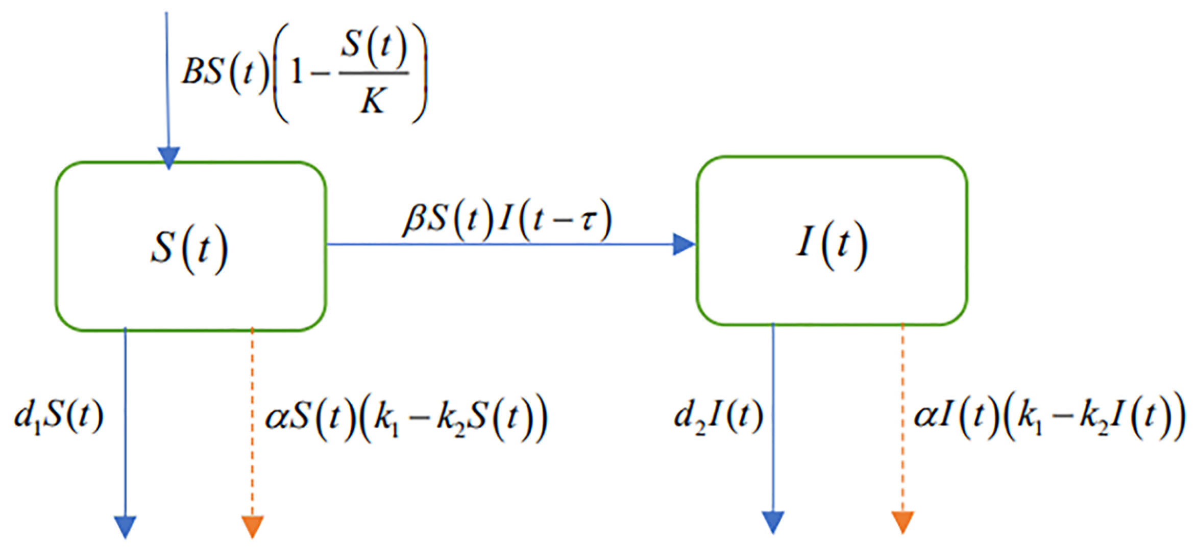
After the outbreak of PWD in an area, we take control measures (such as nematicide injection and vaccination) to protect pine trees. The transmission of PWN is not reliant upon direct contact between M. alternatus, but hinges on the process of infected M. alternatus transmitting PWN to healthy pine trees during feeding and oviposition. Newly formed adult M. alternatus remain within the pupation chamber prior to emergence, where they become infected by PWN from deceased host tree wood, then they carry PWN to continue to infect other healthy pine trees after emergence. Upon implementation of nematicide injection or vaccination, the quantity of PWN in pine trees diminishes, leading to a concomitant decline in infection rate. Therefore, taking control measures on trees can effectively reduce the infection rate of M. alternatus. Moreover, measures such as insecticidal spraying insecticides can kill M. alternatus, which also reduces the rate of infection. However, the transmission speed of PWN is very fast when the forest is in the outbreak period of PWD, so in the early stage of control, the transmission efficiency of PWN may be higher than that of control. Consequently, there is a time delay between taking control measures and the beginning of the decline in the infection rate of M. alternatus, so there is a certain time delay in the effective of prevention and control. Since not every time infected M. alternatus can “feed” PWN, we introduce an infection coefficient. We suppose that the infection coefficient of PWD is reduced to $\beta$ after adopting control measures. Other influencing factors in the infection-control system are analyzed below.

It is assumed that M. alternatus are divided into susceptible M. alternatus $S\left(t\right)$ which did not carry PWN and infected M. alternatus $I\left(t\right)$ which did carry PWN at a certain time in a PWD epidemic area. For the input of M. alternatus, the born M. alternatus and the dead M. alternatus are mainly considered. Because the resources are limited, it is more realistic for us to use the logistic function to describe the growth rate of the M. alternatus. We assume the natural mortality of susceptible and infected M. alternatus as $d_1$, $d_2$, respectively. In the process of the spread of PWD, prevention and control can increase the mortality rate of M. alternatus, thereby inhibiting the spread of the disease. With the progress of control, the mortality rate of M. alternatus will tend to be saturated. Therefore, the number of M. alternatus killed by artificial control grows following nonlinear logistic growth, and the mortality rate of M. alternatus is related to the intensity of control, with the increase of control efforts, the mortality rate also increases nonlinearly, so we use $k_1\alpha$ to describe its linear part and $k_2\alpha$ to describe its nonlinear part, where $k_1\alpha$ represents control measures efficiency of PWD. Adding the nonlinear part better reflects the saturation effect of artificial prevention and control, which is more consistent with reality. To better study the impact of prevention and control on PWD infection-control system, we present the variable relationships shown in Figure 1.

According to Figure 1, we can construct the following delayed differential equation model:

$$\left\{\begin{array}{c}\frac{\mathrm{d}S}{\mathrm{d}t}=B(1-\frac{S\left(t\right)}{K})S\left(t\right)-d_{1}S\left(t\right)-\beta S\left(t\right)I(t-\tau )-k_1\alpha S\left(t\right)+k_2\alpha S^2\left(t\right),\hfill \\ \frac{\mathrm{d}I}{\mathrm{d}t}=\beta S\left(t\right)I(t-\tau )-d_{2}I\left(t\right)-k_1\alpha I\left(t\right)+k_2\alpha I^2\left(t\right),\hfill \end{array}\right.$$

(1)

where $S\left(t\right)$ and $I\left(t\right)$ are the variables; B, $d_1$, $d_2$, $k_1$, $k_2$, $\beta$, $\alpha$ and K are the positive constants; and $\tau$ is the time delay of disease control to take effect. The specific descriptions are given in

Table 1. Descriptions of parameters in the model (1).

Symbol	Description	Unit
S	Amount of susceptible M. alternatus	${10}^4\mathrm{head}$
I	Amount of infected M. alternatus	${10}^4\mathrm{head}$
B	Natural birth rate of M. alternatus	$\% \left(\mathrm{year}\right)$
$d_1$	Natural mortality of susceptible M. alternatus	$\% \left(\mathrm{year}\right)$
$d_2$	Natural mortality of infected M. alternatus	$\% \left(\mathrm{year}\right)$
$k_1$	Linear coefficient related to mortality caused by control	-
$k_2$	Nonlinear coefficient related to mortality caused by control	-
$\beta$	Infection coefficient	-
$\alpha$	Intensity of prevention and control against M. alternatus	%
K	Environmental capacity	-
$\tau$	Time delay of disease control to take effect	year
t	Time	year

.

For convenience, we denote that $n_1=B-d_1-k_1\alpha$, $n_2=k_2\alpha -\frac{B}{K}$, $n_3=d_2+k_1\alpha$; then, model (1) becomes:

$$\left\{\begin{array}{c}\frac{\mathrm{d}S}{\mathrm{d}t}=n_{1}S\left(t\right)+n_2{S}^2\left(t\right)-\beta S\left(t\right)I(t-\tau ),\hfill \\ \frac{\mathrm{d}I}{\mathrm{d}t}=\beta S\left(t\right)I(t-\tau )-n_{3}I\left(t\right)+k_2\alpha I^2\left(t\right).\hfill \end{array}\right.$$

(2)

Due to the wide distribution and strong concealment of M. alternatus, we believe that the number of births of susceptible M. alternatus is always greater than the number of deaths, that is, $n_1>0$, which is also consistent with the data we found in the later parameter analysis. Moreover, we believe that the intensity of prevention and control against M. alternatus will be change within 0∼1, that is, the maximum value of $\alpha$ is 100%.

Then, we prove that the solution of system (2) is nonnegative under positive initial conditions.

The initial condition of system (2) is $\phi =\left({\phi }_s\left(\theta \right),{\phi }_I\left(\theta \right)\right)\in C\left(\left[-\tau ,0\right],R_{+0}^2\right),\theta \in \left[-\tau ,0\right]$, where ${\phi }_s\left(\theta \right)\ge 0$, ${\phi }_I\left(\theta \right)\ge 0$, $C\left(\left[-\tau ,0\right],R_{+0}^2\right)$ is a continuous function mapping from $\left[-\tau ,0\right]$ to $R_{+0}^2$ in Banach space, for system (2), $R_{+0}^2=\left\{(S\left(t\right),I\left(t\right))\right|S\left(t\right)\ge 0,I\left(t\right)\ge 0\}$.

Theorem 1.

If ${\phi }_s\left(\theta \right)\ge 0$, ${\phi }_I\left(\theta \right)\ge 0$, $\theta \in \left[-\tau ,0\right]$, then the solution of system (2) $S\left(t\right)$, $I\left(t\right)$ is nonnegative for $t\ge 0$.

Proof. 

Assume that the system (2) in the nonnegative initial function ${\phi }_s\left(\theta \right)\ge 0$, $\theta \in \left[-\tau ,0\right]$, the solution $S\left(t\right)$ is not nonnegative when $t\ge 0$, then there must be the first time $t_1>0$, such that $S\left(t_1\right)=0$, $S^{\prime }\left(t_1\right)<0$. According to the first equation of system (2), we can obtain $S^{\prime }\left(t_1\right)=0$, contradicting with $S^{\prime }\left(t_1\right)<0$ at this time.

Similarly, assuming that the solution of system (2) $I\left(t\right)$ is not nonnegative when $t\ge 0$ in the case of nonnegative initial function ${\phi }_I\left(\theta \right)\ge 0$, $\theta \in \left[-\tau ,0\right]$, then there must be a first time $t_2>0$, such that $I\left(t_2\right)=0$, $I\left(t_2-\tau \right)>0$, $I^{\prime }\left(t_2\right)<0$, according to the second equation of system (2): $I^{\prime }\left(t_2\right)=\beta SI\left(t_2-\tau \right)$, note the parameter $\beta >0$, so $I^{\prime }\left(t_2\right)>0$, contradicting with $I^{\prime }\left(t_2\right)<0$ at this time.

In summary, when $t\ge 0$, the solutions $S\left(t\right)$ and $I\left(t\right)$ of system (2) are still nonnegative for nonnegative initial functions. □

3. Stability Analysis of Equilibrium and Existence of Hopf Bifurcation

In this section, we will discuss the stability of equilibria and the existence of Hopf bifurcation for system (2).

3.1. Existence of Equilibrium Point

Firstly, we give the following assumptions:

$$\begin{array}{cc}& \left(\mathrm{H}1\right)n_2<0,\hfill \\ & \left(\mathrm{H}2\right)\left\{\begin{array}{c}\frac{(d_2+k_1\alpha )({\beta }^2+k_2\alpha n_2)-k_2\alpha (n_1\beta +n_2{n}_3)}{\beta ({\beta }^2+k_2\alpha n_2)}>0,\hfill \\ \frac{n_1\beta +n_2{n}_3}{{\beta }^2+k_2\alpha n_2}>0.\hfill \end{array}\right.\hfill \end{array}$$

System (2) always has a zero equilibrium $E_1=(S^{\left(1\right)},I^{\left(1\right)})=(0,0)$ and a boundary equilibrium $E_2=(S^{\left(2\right)},I^{\left(2\right)})=(0,\frac{n_3}{k_2\alpha })$, since $n_3>0, k_2\alpha >0$. When $\left(\mathrm{H}1\right)$ holds, system (2) has a disease-free equilibrium:

$$E_3=(S^{\left(3\right)},I^{\left(3\right)})=(-\frac{n_1}{n_2},0).$$

When $\left(\mathrm{H}2\right)$ holds, system (2) has a positive equilibrium:

$$E_4=(S^{\left(4\right)},I^{\left(4\right)})=(\frac{d_2+k_1\alpha -k_2\alpha I^{\left(4\right)}}{\beta },\frac{n_1\beta +n_2{n}_3}{{\beta }^2+k_2\alpha n_2}).$$

Based on the practical significance, we pay more attention to the existence and stability of disease-free equilibrium $E_3$ and positive equilibrium $E_4$.

Remark 1.

If $n_2=k_2\alpha -\frac{B}{K}<0$, that is $k_2\alpha <\frac{B}{K}$. When $k_2$, α, B are fixed, the smaller K is, the greater possibility of the assumption $\left(\mathrm{H}1\right)$ is established. Therefore, when the natural conditions of a forest area are better, that is, the environmental carrying capacity of M. alternatus is large, the assumption $\left(\mathrm{H}1\right)$ may not hold, and thus, the disease-free equilibrium $E_3$ may not exist. This indicates that when the forest conditions are suitable for the survival of M. alternatus, the infected M. alternatus cannot be completely eliminated, which is consistent with the actual situation.

Next, we will discuss the existence and stability of equilibrium $E_3,E_4$.

3.2. Stability and Existence of Hopf Bifurcation for $E_3$

When $\left(\mathrm{H}1\right)$ holds, system (2) has a disease-free equilibrium $E_3$. Transferring the equilibrium $E_3$ to the origin and linearizing the surrounding system (2), we obtain the characteristic equation of the linearized system as follows:

$$\left(\lambda +n_1\right)\left(\lambda +n_3+\frac{\beta n_1}{n_2}{\mathrm{e}}^{-\lambda \tau }\right)=0.$$

(3)

When $\tau =0$, Equation (3) becomes:

$$\left(\lambda +n_1\right)\left(\lambda +\frac{\beta n_1+n_2{n}_3}{n_2}\right)=0.$$

(4)

Then, We give the following hypothesis:

$$\left(\mathrm{H}3\right)\beta n_1+n_2{n}_3<0.$$

Equation (4) has two characteristic roots ${\lambda }_1=-n_1$, ${\lambda }_2=-\frac{\beta n_1+n_2{n}_3}{n_2}$. Since $n_2<0$, when $\left(\mathrm{H}3\right)$ holds, ${\lambda }_1<0$ and ${\lambda }_2<0$, then $E_3$ is locally asymptotically stable; when $\beta n_1+n_2{n}_3=0$, ${\lambda }_2=0$, the equilibrium $E_3$ undergoes a fixed point bifurcation; when $\beta n_1+n_2{n}_3>0$, ${\lambda }_1<0$ but ${\lambda }_2>0$, and thus, the equilibrium $E_3$ is unstable at this time.

When $\tau >0$, we try to discuss the existence of Hopf bifurcation. We assume that $\lambda =\mathrm{i}\omega (\omega >0)$ is a pure imaginary root of Equation (3). Substituting it into Equation (3) and separating the real and imaginary parts, we obtain:

$$\left\{\begin{array}{c}\hfill {\omega }^2-n_1{n}_3=\frac{\beta n_1^2}{n_2}cos\left(\omega \tau \right)+\frac{\beta n_1\omega }{n_2}sin\left(\omega \tau \right),\\ \hfill \left(n_1+n_3\right)\omega =\frac{\beta n_1^2}{n_2}sin\left(\omega \tau \right)-\frac{\beta n_1\omega }{n_2}cos\left(\omega \tau \right).\end{array}\right.$$

(5)

Equation (5) derives the following results:

$$\begin{array}{cc}\hfill sin\left(\omega \tau \right)& =\frac{n_2\left(\beta n_1{\omega }^3+\beta n_1^3\omega \right)}{{\beta }^2{n}_1^4+{\beta }^2{n}_1^2{\omega }^2}\triangleq X_0,\hfill \\ \hfill cos\left(\omega \tau \right)& =\frac{-n_2\left(\beta n_1^3{n}_3+\beta n_1{n}_3{\omega }^2\right)}{{\beta }^2{n}_1^4+{\beta }^2{n}_1^2{\omega }^2}\triangleq Y_0.\hfill \end{array}$$

(6)

Adding the square of the two equations in Equation (5), letting ${\omega }^2=z$, we obtain:

$$h\left(z\right)=z^2+\frac{n_1^2{n}_2^2+n_2^2{n}_3^2-{\beta }^2{n}_1^2}{n_2^2}z+\frac{n_1^2\left(n_2^2{n}_3^2-{\beta }^2{n}_1^2\right)}{n_2^2}.$$

(7)

When $\left(\mathrm{H}3\right)$ holds, ${\beta }^2{n}_1^2<n_2^2{n}_3^2$, Equation (7) has no positive root, the equilibrium $E_3$ is locally asymptotically stable for any $\tau >0$; when $\beta n_1+n_2{n}_3=0$, ${\beta }^2{n}_1^2=n_2^2{n}_3^2$, Equation (7) also only has a zero root and no pair of pure imaginary roots, and thus, the equilibrium $E_3$ still undergoes a fixed point bifurcation; when $\beta n_1+n_2{n}_3>0$, ${\beta }^2{n}_1^2>n_2^2{n}_3^2$, Equation (7) always has one positive root $z_0$. From Equation (6), we can solve the critical value of time delay:

$${\tau }_0^{\left(j\right)}=\left\{\begin{array}{c}\frac{arccos{Y}_0+2j\pi }{{\omega }_0}, X_0>0,\hfill \\ \frac{2\pi -arccos{Y}_0+2j\pi }{{\omega }_0}, X_0\le 0, j=0,1,2,\cdots ,\hfill \end{array}\right.$$

(8)

where $X_0$ and $Y_0$ are given in Equation (6).

Lemma 1.

If $\left(\mathrm{H}1\right)$ holds and $\beta n_1+n_2{n}_3>0$, when $\tau ={\tau }_0^{\left(j\right)}(j=0,1,2,\cdots )$, then Equation (3) has a pair of pure imaginary roots $\pm \mathrm{i}{\omega }_0$, and all the other roots of Equation (3) have nonzero real parts.

Let $\lambda =\lambda \left(\tau \right)$ be the root of Equation (3), satisfying $\lambda \left({\tau }_0^{\left(j\right)}\right)=\mathrm{i}{\omega }_0(j=0,1,2,\cdots )$. Then, we will calculate transversality condition.

Lemma 2.

If $\left(\mathrm{H}1\right)$ holds and $\beta n_1+n_2{n}_3>0$, Equation (7) has one positive root $z_0$ and $z_0={\omega }_0^2$, $h^{\prime }\left(z_0\right)>0$, where $h^{\prime }\left(z\right)$ is the derivative of $h\left(z\right)$ with respect to z. Then, we have the following transversality condition:

$${\left.Re{\left(\frac{\mathrm{d}\lambda }{\mathrm{d}\tau }\right)}^{-1}\right|}_{\tau ={\tau }_0^{\left(j\right)}}=\frac{n_2^2{h}^{\prime }\left(z_0\right)}{{\beta }^2{n}_1^2\left(n_1^2+z_0\right)}>0.$$

Therefore, when $\left(\mathrm{H}1\right)$ holds and $\beta n_1+n_2{n}_3>0$, system (2) undergoes a Hopf bifurcation near equilibrium $E_3$.

Theorem 2.

If the parameters of system (2) meet $\left(\mathrm{H}1\right)$, then:

(1) 

When $\left(\mathrm{H}3\right)$ holds, the equilibrium $E_3$ is locally asymptotically stable for any $\tau \ge 0$.

(2) 

When $\left(\mathrm{H}3\right)$ does not hold, if $\beta n_1+n_2{n}_3=0$, the equilibrium $E_3$ undergoes a fixed point bifurcation for any $\tau \ge 0$; if $\beta n_1+n_2{n}_3>0$, it is unstable for any $\tau \ge 0$ and system (2) undergoes a Hopf bifurcation near equilibrium $E_3$ when $\tau ={\tau }_0^{\left(j\right)}$.

3.3. Stability and Existence of Hopf Bifurcation for $E_4$

Next, we analyze the stability of system (2) for $E_4=(S^{\left(4\right)},I^{\left(4\right)})$. Similarly, transferring the equilibrium $E_4$ to the origin and linearizing the system (2) around it, we obtain the characteristic equation of the linearized system as follows:

$${\lambda }^2+\left(a_1-\beta S^{\left(4\right)}{\mathrm{e}}^{-\lambda \tau }\right)\lambda +a_2+a_3{\mathrm{e}}^{-\lambda \tau }=0.$$

(9)

where

$$\begin{array}{cc}& a_1=n_3-2k_2\alpha I^{\left(4\right)}-n_2{S}^{\left(4\right)},\hfill \\ & a_2=2n_2{k}_2\alpha S^{\left(4\right)}{I}^{\left(4\right)}-n_2{n}_3{S}^{\left(4\right)},\hfill \\ & a_3=n_2\beta {\left(S^{\left(4\right)}\right)}^2+{\beta }^2{S}^{\left(4\right)}{I}^{\left(4\right)}.\hfill \end{array}$$

When $\tau =0$, Equation (9) becomes:

$${\lambda }^2+\left(a_1-\beta S^{\left(4\right)}\right)\lambda +a_2+a_3=0.$$

(10)

We consider the following assumption obtained by Vieta theorem:

$$\left(\mathrm{H}4\right)\left\{\begin{array}{c}\beta {\mathrm{S}}^{\left(4\right)}-{\mathrm{a}}_1<0,\hfill \\ {\mathrm{a}}_2+{\mathrm{a}}_3>0.\hfill \end{array}\right.$$

Under the assumption $\left(\mathrm{H}4\right)$, all the roots of Equation (10) have negative real parts, and the equilibrium $E_4=(S^{\left(4\right)},I^{\left(4\right)})$ is locally asymptotically stable when $\tau =0$.

When $\tau >0$, we will discuss the existence of Hopf bifurcation. We assume that $\lambda =\mathrm{i}\omega (\omega >0)$ is a pure imaginary root of Equation (9). Substituting it into Equation (9) and separating the real and imaginary parts, we obtain:

$$\left\{\begin{array}{c}{a}_1\omega =a_{3}sin\left(\omega \tau \right)+\beta S^{\left(4\right)}\omega cos\left(\omega \tau \right),\hfill \\ {\omega }^2-a_2=a_{3}cos\left(\omega \tau \right)-\beta S^{\left(4\right)}\omega sin\left(\omega \tau \right).\hfill \end{array}\right.$$

(11)

Equation (11) derives the following results:

$$\begin{array}{cc}\hfill sin\left(\omega \tau \right)& =\frac{a_1{a}_3\omega +\beta S^{\left(4\right)}{a}_2\omega -\beta S^{\left(4\right)}{\omega }^3}{a_3^2+{\beta }^2{\left(S^{\left(4\right)}\right)}^2{\omega }^2}\triangleq X_1,\hfill \\ \hfill cos\left(\omega \tau \right)& =\frac{a_3{\omega }^2-a_2{a}_3+\beta S^{\left(4\right)}{a}_1{\omega }^2}{a_3^2+{\beta }^2{\left(S^{\left(4\right)}\right)}^2{\omega }^2}\triangleq Y_1.\hfill \end{array}$$

(12)

Adding the square of the two equations in Equation (11), letting ${\omega }^2=z$, we obtain:

$$l\left(z\right)=z^2+A_{1}z+A_2=0,$$

(13)

where $A_1=a_1^2-2a_2-{\beta }^2{\left(S^{\left(4\right)}\right)}^2$ and $A_2=a_2^2-a_3^2$. Then, if $A_1>0$ and $A_2>0$ hold, Equation (13) has no positive root; if $A_2<0$ holds, Equation (13) has one positive root $z_1$; if $A_1<0$ and $A_2>0$ hold, Equation (13) has two positive roots $z_2,z_3$. We hypothesize that Equation (13) has positive roots $z_n(n=1,2,3)$, then ${\omega }_n=\sqrt{z_n}(n=1,2,3)$. From Equation (12), we can solve the critical value of time delay:

$${\tau }_n^{\left(j\right)}=\left\{\begin{array}{c}\frac{arccos{Y}_1+2j\pi }{{\omega }_n}, X_1>0,\hfill \\ \frac{2\pi -arccos{Y}_1+2j\pi }{{\omega }_n}, X_1\le 0, n=1,2,3, j=0,1,2,\cdots ,\hfill \end{array}\right.$$

(14)

where $X_1$ and $Y_1$ are given in Equation (12).

Lemma 3.

When $\left(\mathrm{H}2\right)$ and $\left(\mathrm{H}4\right)$ hold, if $A_2<0$ or $A_1<0,A_2>0$, where $A_1$ and $A_2$ are given in Equation (13), when $\tau ={\tau }_n^{\left(j\right)}(n=1,2,3, j=0,1,2,\cdots )$, then Equation (9) has a pair of pure imaginary roots $\pm \mathrm{i}{\omega }_n$, and all the other roots of Equation (9) have nonzero real parts.

Let $\lambda =\lambda \left(\tau \right)$ be the root of Equation (9), satisfying $\lambda ({\tau }_n^{\left(j\right)})=\mathrm{i}{\omega }_n(n=1,2,3)$. Then, we will calculate transversality condition.

Lemma 4.

When $\left(\mathrm{H}2\right)$ and $\left(\mathrm{H}4\right)$ hold, if $A_2<0$ or $A_1<0,A_2>0$, where $A_1$, $A_2$ are given in Equation (13), and $z_n={\omega }_n^2$, $l^{\prime }\left(z_n\right)\ne 0(n=1,2,3)$, where $l^{\prime }\left(z\right)$ is the derivative of $l\left(z\right)$ with respect to z. Then, we have the following transversality condition:

$${\left.Re{\left(\frac{\mathrm{d}\lambda }{\mathrm{d}\tau }\right)}^{-1}\right|}_{\tau ={\tau }_n^{\left(j\right)}}=\frac{l^{\prime }\left(z_n\right)}{{\beta }^2{\left(S^{\left(4\right)}\right)}^2{z}_n+a_3^2}\ne 0.$$

Theorem 3.

When $\left(\mathrm{H}2\right)$ holds, system (2) has a positive equilibrium $E_4$. When $\left(\mathrm{H}4\right)$ holds as well:

(1) 

If $A_1>0$, $A_2>0$ hold, Equation (13) has no positive root, the equilibrium $E_4$ is locally asymptotically stable for any $\tau \ge 0$;

(2) 

If $A_2<0$ holds, Equation (13) has one positive roots $z_1$, then when $\tau \in [0,{\tau }_1^{\left(0\right)})$, the equilibrium $E_4$ is locally asymptotically stable, and unstable when $\tau >{\tau }_1^{\left(0\right)}$, and it undergoes a Hopf bifurcation when $\tau ={\tau }_1^{\left(j\right)}, j=0,1,2,\cdots$;

(3) 

If $A_1<0$, $A_2>0$ hold, system (2) undergoes a Hopf bifurcation near the equilibrium $E_4$ when $\tau ={\tau }_n^{\left(j\right)},n=2,3, j=0,1,2,\cdots$. Then, $\exists m\in N$ makes $0<{\tau }_3^{\left(0\right)}<{\tau }_2^{\left(0\right)}<{\tau }_3^{\left(1\right)}<{\tau }_2^{\left(1\right)}<\cdots <{\tau }_2^{\left(m-1\right)}<{\tau }_3^{\left(m\right)}<{\tau }_3^{\left(m+1\right)}$. When $\tau \in \left[0,{\tau }_3^{\left(0\right)}\right)\bigcup {\displaystyle \bigcup _{l=1}^m}\left({\tau }_2^{\left(l-1\right)},{\tau }_3^{\left(l\right)}\right)$, the equilibrium $E_4$ of the system (2) is locally asymptotically stable, and when $\tau \in {\displaystyle \bigcup _{l=0}^{m-1}}\left({\tau }_3^{\left(l\right)},{\tau }_2^{\left(l\right)}\right)\bigcup \left({\tau }_3^{\left(m\right)},+\infty \right)$, the equilibrium $E_4$ is unstable.

4. Normal Form of Hopf Bifurcation

In Section 3, we have shown that when $\beta n_1+n_2{n}_3<0$, the equilibrium $E_3$ is locally asymptotically stable for any $\tau \ge 0$; when $\beta n_1+n_2{n}_3>0$, the bifurcating periodic solution near the equilibrium $E_3$ is unstable by Theorem 2. Thus, we only care about the stability of bifurcating periodic solution near the positive equilibrium $E_4$. In order to be more realistic, we focus on the delay between taking control measures and the beginning of control to take effect. Therefore, we consider the time-delay $\tau$ as a bifurcation parameter and denote the critical value $\tau ={\tau }_c={\tau }_n^{\left(j\right)}$, where ${\tau }_n^{\left(j\right)}$ is given in Equation (14). When $\tau ={\tau }_n^{\left(j\right)}$, Equation (13) has a pair of pure imaginary roots $\lambda =\pm \mathrm{i}\omega$. Therefore, system (2) undergoes a Hopf bifurcation near equilibrium $E_4$. In this section, we derive the normal form of Hopf bifurcation for the system (2) by using the multiple time scales method.

In order to normalize the delay, we first re-scale the time t by using $t\mapsto t/\tau$, then translate the equilibrium $E_4=(S^{\left(4\right)},I^{\left(4\right)})=(\frac{d_2+k_1\alpha -k_2\alpha I^{\left(4\right)}}{\beta },\frac{n_1\beta +n_2{n}_3}{{\beta }^2+k_2\alpha n_2})$ to the origin, so system (2) is transformed into:

$$\left\{\begin{array}{c}\frac{\mathrm{d}S}{\mathrm{d}t}=\tau [(n_1+2n_2{S}^{\left(4\right)}-\beta I^{\left(4\right)})S\left(t\right)+n_2{S}^2\left(t\right)-\beta (S\left(t\right)+S^{\left(4\right)})I(t-1)],\hfill \\ \frac{\mathrm{d}I}{\mathrm{d}t}=\tau [(2k_2\alpha I^{\left(4\right)}-n_3)I\left(t\right)+k_2\alpha I^2\left(t\right)+\beta I^{\left(4\right)}S\left(t\right)+\beta (S\left(t\right)+S^{\left(4\right)})I(t-1)].\hfill \end{array}\right.$$

(15)

Equation (15) can also be written as:

$$\dot{Z\left(t\right)}=\tau N_{1}Z\left(t\right)+\tau N_{2}Z(t-1)+\tau F\left(Z\right(t),Z(t-1\left)\right),$$

(16)

where

$$Z\left(t\right)={\left(S\right(t),I(t\left)\right)}^T,Z(t-1)={\left(S\right(t-1),I(t-1\left)\right)}^T,$$

and

$$\begin{array}{cc}& N_1=\left(\begin{array}{cc}{n}_1+2n_2{S}^{\left(4\right)}-\beta I^{\left(4\right)}& 0\\ \beta I^{\left(4\right)}& 2k_2\alpha I^{\left(4\right)}-n_3\end{array}\right),N_2=\left(\begin{array}{cc}0& -\beta S^{\left(4\right)}\\ 0& \beta S^{\left(4\right)}\end{array}\right),\hfill \\ & F\left(Z\left(t\right),Z\left(t-1\right)\right)=\left(\begin{array}{c}{n}_{2}S{}^2\left(t\right)-\beta S\left(t\right)I\left(t-1\right)\hfill \\ k_2\alpha I{}^2\left(t\right)+\beta S\left(t\right)I\left(t-1\right)\hfill \end{array}\right).\hfill \end{array}$$

Let h be eigenvector corresponding to eigenvalue $\lambda =\mathrm{i}\omega \tau$ of linearized system of Equation (16), and $h^{*}$ be the eigenvector corresponding to eigenvalue $\lambda =-\mathrm{i}\omega \tau$ of adjoint matrix of linearized system of Equation (16), satisfying:

$$\langle h^{*},h\rangle ={\overline{h^{*}}}^{T}h=1.$$

(17)

By calculating, we have:

$$\left\{\begin{array}{c}h={(h_{11},h_{12})}^T={(1,\frac{n_2{S}^{\left(4\right)}-\mathrm{i}\omega }{\beta S^{\left(4\right)}{\mathrm{e}}^{-\mathrm{i}\omega \tau }})}^T,\hfill \\ h^{*}=d{(h_{21},h_{22})}^T=d{(\frac{\mathrm{i}\omega -n_3+2k_2\alpha I^{\left(4\right)}+\beta S^{\left(4\right)}{\mathrm{e}}^{\mathrm{i}\omega \tau }}{\beta S^{\left(4\right)}{\mathrm{e}}^{\mathrm{i}\omega \tau }},1)}^T,\hfill \end{array}\right.$$

(18)

where $d={(\overline{h_{11}}{h}_{21}+\overline{h_{12}}{h}_{22})}^{-1}$.

We suppose the solution of Equation (16) is as follows:

$$Z\left(t\right)=Z(T_0,T_1,T_2,\cdots )=\sum _{k=1}^{+\infty }{\epsilon }^k{Z}_k\left(T_0,T_1,T_2\cdots \right),$$

(19)

where

$$\begin{array}{c}Z(T_0,T_1,T_2,\cdots )={(S(T_0,T_1,T_2,\cdots ),I(T_0,T_1,T_2,\cdots ))}^T,\hfill \\ Z_k(T_0,T_1,T_2,\cdots )={(S_k(T_0,T_1,T_2,\cdots ),I_k(T_0,T_1,T_2,\cdots ))}^T.\hfill \end{array}$$

The derivative with respect to t is transformed:

$$\frac{\mathrm{d}}{\mathrm{d}t}=\frac{\partial }{\partial T_0}+\epsilon \frac{\partial }{\partial T_1}+{\epsilon }^2\frac{\partial }{\partial T_2}+\cdots =D_0+\epsilon D_1+{\epsilon }^2{D}_2+\cdots ,$$

(20)

where $D_i$ is differential operator, and:

$$D_i=\frac{\partial }{\partial T_i}\left(i=0,1,2\cdots \right).$$

Note that:

$$\begin{array}{c}{Z}_i={\left(S_i,I_i\right)}^T=Z_i\left(t,\epsilon t,{\epsilon }^{2}t,\cdots \right),\hfill \\ Z_{i1}={\left(S_i,I_i\right)}^T=Z_i\left(t-1,\epsilon t,{\epsilon }^{2}t,\cdots \right),i=1,2,\cdots .\hfill \end{array}$$

Then, we obtain:

$$\dot{Z}\left(t\right)=\epsilon D_0{Z}_1+{\epsilon }^2{D}_1{Z}_1+{\epsilon }^3{D}_2{Z}_1+{\epsilon }^2{D}_0{Z}_2+{\epsilon }^3{D}_1{Z}_2+{\epsilon }^3{D}_0{Z}_3+\cdots .$$

(21)

Using a Taylor series expansion of $Z(t-1)$, we obtain: that

$$Z\left(t-1\right)=\epsilon Z_{11}+{\epsilon }^2\left(Z_{21}-D_1{Z}_{11}\right)+{\epsilon }^3\left(Z_{31}-D_1{Z}_{21}-D_2{Z}_{11}\right)+\cdots ,$$

(22)

where $Z_{i1}=Z_i\left(T_0-1,T_1,T_2,\cdots \right), i=1,2,3,\cdots$.

As we stated, $\tau$ is the bifurcation parameter, and $\tau ={\tau }_c+\epsilon \mu$, where ${\tau }_c={\tau }_n^{\left(j\right)}$$(j=0,1,2,\cdots )$ is the Hopf bifurcation critical value, $\mu$ is perturbation parameter, and $\epsilon$ is dimensionless scale parameter. Substituting Equations (19)–(22) into Equation (16) and balancing the coefficients before $\epsilon$ on both sides of the equation, the following expression is obtained:

$$\left\{\begin{array}{c}{D}_0{S}_1={\tau }_c[(n_1+2n_2{S}^{\left(4\right)}-\beta I^{\left(4\right)})S_1-\beta S^{\left(4\right)}{I}_{11}],\hfill \\ D_0{I}_1={\tau }_c[(2k_2\alpha I^{\left(4\right)}-n_3)I_1+\beta S^{\left(4\right)}{I}_{11}].\hfill \end{array}\right.$$

(23)

Thus, Equation (23) has the following solution form:

$$Z\left(T_1,T_2,T_3,\cdots \right)=G\left(T_1,T_2,T_3,\cdots \right){\mathrm{e}}^{\mathrm{i}\omega {\tau }_c{T}_0}h+\overline{G}\left(T_1,T_2,T_3,\cdots \right){\mathrm{e}}^{-\mathrm{i}\omega {\tau }_c{T}_0}\overline{h}.$$

(24)

The expression of the coefficient before ${\epsilon }^2$ is as follows:

$$\left\{\begin{array}{c} D_0{S}_2-{\tau }_c[(n_1+2n_2{S}^{\left(4\right)}-\beta I^{\left(4\right)})S_2-\beta S^{\left(4\right)}{I}_{21}]\hfill \\ =-D_1{S}_1+{\tau }_c[n_2{S}_1^2-\beta S_1{I}_{11}+\beta S^{\left(4\right)}{D}_1{I}_{11}]+\mu [(n_1+2n_2{S}^{\left(4\right)}-\beta I^{\left(4\right)})S_1-\beta S^{\left(4\right)}{I}_{11}],\hfill \\ D_0{I}_2-{\tau }_c[(2k_2\alpha I^{\left(4\right)}-n_3)I_2+\beta I^{\left(4\right)}{S}_2+\beta S^{\left(4\right)}{I}_{21}]\hfill \\ =-D_1{I}_1+{\tau }_c[k_2\alpha I_1^2++\beta S_1{I}_{11}-\beta S^{\left(4\right)}{D}_1{I}_{11}]+\mu [(2k_2\alpha I^{\left(4\right)}-n_3)I_1+\beta S^{\left(4\right)}{I}_{11}].\hfill \end{array}\right.$$

(25)

Substituting Equation (24) into the right-hand side of Equation (25), and the coefficient vector of ${\mathrm{e}}^{\mathrm{i}\omega {\tau }_c{T}_0}$ is denoted by $m_1$. According to the solvability condition $\langle h^{*},m_1\rangle =0$, the expression of $\frac{\partial G}{\partial T_1}$ is obtained as follows:

$$\frac{\partial G}{\partial T_1}=\mu MG,$$

(26)

where $M=\frac{\overline{h_{21}}\left[\left(n_1+2n_2{S}^{\left(4\right)}-\beta I^{\left(4\right)}\right)h_{11}-\beta S^{\left(4\right)}{\mathrm{e}}^{-\mathrm{i}\omega {\tau }_c}{h}_{12}\right]+\overline{h_{22}}\left[\left(2k_2\alpha -n_3\right)h_{12}+\beta S^{\left(4\right)}{\mathrm{e}}^{-\mathrm{i}\omega {\tau }_c}{h}_{12}\right]}{\overline{h_{21}}\left(h_{11}-\beta S^{\left(4\right)}{\tau }_c{\mathrm{e}}^{-\mathrm{i}\omega {\tau }_c}{h}_{12}\right)+\overline{h_{22}}\left(h_{12}+\beta S^{\left(4\right)}{\tau }_c{\mathrm{e}}^{-\mathrm{i}\omega {\tau }_c}{h}_{12}\right)}$.

Since $\mu$ is a disturbance parameter, we only consider its effect on the linear part. Therefore, we ignore the part containing $\mu$ in the higher order. We suppose the solutions of Equation (25) are given as follows:

$$\left\{\begin{array}{c}{S}_2={\eta }_{0}G\overline{G}+{\eta }_1{\mathrm{e}}^{2\mathrm{i}\omega {\tau }_c{T}_0}{G}^2+\overline{{\eta }_1}{\mathrm{e}}^{-2\mathrm{i}\omega {\tau }_c{T}_0}\overline{G^2},\hfill \\ I_2={\xi }_{0}G\overline{G}+{\xi }_1{\mathrm{e}}^{2\mathrm{i}\omega {\tau }_c{T}_0}{G}^2+\overline{{\xi }_1}{\mathrm{e}}^{-2\mathrm{i}\omega {\tau }_c{T}_0}\overline{G^2},\hfill \end{array}\right.$$

(27)

where

$$\begin{array}{c}\left(\begin{array}{c}{\eta }_0\hfill \\ {\xi }_0\hfill \end{array}\right)=V_0\left(\begin{array}{cc}{n}_3-2k_2\alpha I^{\left(4\right)}-\beta S^{\left(4\right)}& \beta S^{\left(4\right)}\\ \beta I^{\left(4\right)}& \beta I^{\left(4\right)}-n_1-2n_2{S}^{\left(4\right)}\end{array}\right)\left(\begin{array}{c}{x}_0\hfill \\ y_0\hfill \end{array}\right),\hfill \\ \left(\begin{array}{c}{\eta }_1\hfill \\ {\xi }_1\hfill \end{array}\right)=V_1\left(\begin{array}{cc}2i\omega -2k_2\alpha I^{\left(4\right)}+n_3-\beta S^{\left(4\right)}{\mathrm{e}}^{-2\mathrm{i}\omega {\tau }_c}& \beta S^{\left(4\right)}{\mathrm{e}}^{\mathrm{i}\omega {\tau }_c}\\ \beta I^{\left(4\right)}& 2i\omega -n_1-2n_2{S}^{\left(4\right)}{I}^{\left(4\right)}{\mathrm{e}}^{\mathrm{i}\omega {\tau }_c}\end{array}\right)\left(\begin{array}{c}{x}_1\hfill \\ y_1\hfill \end{array}\right),\hfill \end{array}$$

(28)

where $h_{11},h_{12},h_{21},h_{22}$ are given in Equation (18) and

$$\begin{array}{c}{x}_0=2n_2\overline{h_{11}}{h}_{11}-\beta \overline{h_{12}}{h}_{11}{\mathrm{e}}^{\mathrm{i}\omega {\tau }_c}-\beta \overline{h_{11}}{h}_{12}{\mathrm{e}}^{-\mathrm{i}\omega {\tau }_c},\hfill \\ y_0=2k_2\alpha \overline{h_{12}}{h}_{12}+\beta \overline{h_{12}}{h}_{11}{\mathrm{e}}^{\mathrm{i}\omega {\tau }_c}+\beta \overline{h_{11}}{h}_{12}{\mathrm{e}}^{-\mathrm{i}\omega {\tau }_c},\hfill \\ x_1=n_2{h}_{11}^2-\beta h_{11}{h}_{12}{\mathrm{e}}^{-\mathrm{i}\omega {\tau }_c},y_1=k_2\alpha h_{12}^2+\beta h_{11}{h}_{12}{\mathrm{e}}^{-\mathrm{i}\omega {\tau }_c},\hfill \\ V_0={\left[\left(\beta I^{\left(4\right)}-n_1-2n_2{S}^{\left(4\right)}\right)\left(n_3-2k_2\alpha I^{\left(4\right)}-\beta S^{\left(4\right)}\right)-{\beta }^2{S}^{\left(4\right)}{I}^{\left(4\right)}\right]}^{-1},\hfill \\ V_1={\left[\left(2\mathrm{i}\omega -n_1-2n_2{S}^{\left(4\right)}{I}^{\left(4\right)}{\mathrm{e}}^{\mathrm{i}\omega {\tau }_c}\right)\left(2i\omega -2k_2\alpha I^{\left(4\right)}+n_3-\beta S^{\left(4\right)}{\mathrm{e}}^{-2\mathrm{i}\omega {\tau }_c}\right)-{\beta }^2{S}^{\left(4\right)}{I}^{\left(4\right)}{\mathrm{e}}^{\mathrm{i}\omega {\tau }_c}\right]}^{-1}.\hfill \end{array}$$

The expression of the coefficient before ${\epsilon }^3$ is:

$$\left\{\begin{array}{c} D_0{S}_3-{\tau }_c[(n_1+2n_2{S}^{\left(4\right)}-\beta I^{\left(4\right)})S_3-\beta S_3-\beta S^{\left(4\right)}{I}_{31}]\hfill \\ =-D_1{S}_2-D_2{S}_1+{\tau }_c[2n_2{S}_1{S}_2-\beta (S_1{I}_{21}+S_2{I}_{11}-S^{\left(4\right)}{D}_1{I}_{21}-S^{\left(4\right)}{D}_2{I}_{11})]\hfill \\ +\mu [(n_1+2n_2{S}^{\left(4\right)}-\beta I^{\left(4\right)})S_2+n_2{S}_1^2-\beta S_1{I}_{11}-\beta S^{\left(4\right)}(I_{21}-D_1{I}_{11})],\hfill \\ D_0{I}_3-{\tau }_c[(2k_2\alpha I^{\left(4\right)}-n_3)I_3+\beta I^{\left(4\right)}{S}_3+\beta S_3+\beta S^{\left(4\right)}{I}_{31}]\hfill \\ =-D_1{I}_2-D_2{I}_1+{\tau }_c[2k_2\alpha I_1{I}_2+\beta (S_1{I}_{21}+S_2{I}_{11}-S^{\left(4\right)}{D}_1{I}_{21}-S^{\left(4\right)}{D}_2{I}_{11})]\hfill \\ +\mu [(2k_2\alpha I^{\left(4\right)}-n_3)I_2+k_2\alpha I_1^2+\beta I^{\left(4\right)}{S}_2+\beta S_1{I}_{11}+\beta S^{\left(4\right)}(I_{21}-D_1{I}_{11})].\hfill \end{array}\right.$$

(29)

Next, substituting solution (24) and (27) into Equation (29), and with the coefficient vector of ${\mathrm{e}}^{\mathrm{i}\omega {\tau }_c{T}_0}$ noted as $m_2$, by solvability condition, we have $\langle h^{*},m_2\rangle =0$. Note that $\mu$ is a disturbance parameter, and ${\mu }^2$ has little influence for small unfolding parameter, and thus, we can ignore the ${\mu }^{2}G$, then the expression of $\frac{\partial G}{\partial T_2}$ can be obtained as follows:

$$\frac{\partial G}{\partial T_2}=H{G}^2\overline{G},$$

(30)

where

$$\begin{array}{c}H=P{\left(\begin{array}{c}Q-2{\tau }_c{n}_2{\eta }_0{h}_{11}\hfill \\ Q+2{\tau }_c{k}_2\alpha \left({\xi }_0{h}_{12}+{\xi }_1\overline{h_{12}}\right)\hfill \end{array}\right)}^T\left(\begin{array}{c}\overline{h_{21}}\hfill \\ -\overline{h_{22}}\hfill \end{array}\right),\hfill \\ \begin{array}{c}P={\left[\overline{h_{21}}\left(2\beta S^{\left(4\right)}{\tau }_c{\mathrm{e}}^{-\mathrm{i}\omega {\tau }_c}{h}_{12}-h_{11}\right)-\overline{h_{22}}\left(2\beta S^{\left(4\right)}{\tau }_c{\mathrm{e}}^{-\mathrm{i}\omega {\tau }_c}{h}_{12}+h_{12}\right)\right]}^{-1},\hfill \\ Q=\beta {\tau }_c\left({\xi }_0{h}_{11}+{\xi }_1\overline{h_{11}}{\mathrm{e}}^{-2\mathrm{i}\omega {\tau }_c}+{\eta }_0{h}_{12}{\mathrm{e}}^{-\mathrm{i}\omega {\tau }_c}+{\eta }_1\overline{h_{12}}{\mathrm{e}}^{\mathrm{i}\omega {\tau }_c}\right),\hfill \end{array}\hfill \end{array}$$

where $h_{11},h_{12},h_{21},h_{22}$ are given in Equation (18), and ${\xi }_0,{\eta }_0,{\xi }_1,{\eta }_1$ are given in Equation (28).

Let $G\mapsto G/\epsilon$, then, the deduced third-order normal form of Hopf bifurcation of system (2) is:

$$\dot{G}=\mu MG+H{G}^2\overline{G},$$

(31)

where M is given in (26) and H is given in (30).

Substituting $G=r{\mathrm{e}}^{\mathrm{i}\theta }$ into Equation (31), the following normal form of Hopf bifurcation in polar coordinates is obtained:

$$\left\{\begin{array}{c}\dot{r}=\mathrm{Re}\left(M\right)\mu r+\mathrm{Re}\left(H\right)r^3,\hfill \\ \dot{\theta }=\mathrm{Im}\left(M\right)\mu +\mathrm{Im}\left(H\right)r^2.\hfill \end{array}\right.$$

(32)

According to the normal form of Hopf bifurcation in polar coordinates, we only need to consider the first equation in system (32). Thus, the following theorem holds:

Theorem 4.

For the system (32), when $\frac{\mathrm{Re}\left(M\right)\mu }{\mathrm{Re}\left(H\right)}<0$, there is a semitrivial fixed point $r=\sqrt{-\frac{\mathrm{Re}\left(M\right)\mu }{\mathrm{Re}\left(H\right)}}$, and system (2) has periodic solution.

(1) 

If $\mathrm{Re}\left(M\right)\mu <0$, then the periodic solution reduced on the center manifold is unstable.

(2) 

If $\mathrm{Re}\left(M\right)\mu >0$, then the periodic solution reduced on the center manifold is stable.

5. Numerical Simulations

In this part, we first analyze the reasonable values of the parameters based on the existing practical research and then we give numerical simulation based on the selected parameters by using Matlab software (R2021a). Finally, we draw some conclusions according to the simulation results, providing practical guidance for the prevention and control of PWD.

5.1. Determination of Parameter Values

5.1.1. Parameter Analysis of Mortality $d_1,d_2$

Firstly, Ref. [24] provides us with the relationship between the longevity of M. alternatus and the number of PWN carried, as shown in

Table 2. Longevity and the number of PWN carried of M. alternatus.

No.	Quantity of PWN Carried/Pieces	Longevity of M. alternatus/d
1	131	30
2	425	42
3	4904	39
4	3031	39
5	3633	39
6	206	30
7	13,232	30
8	8324	45
9	2339	45
10	1209	42
11	1860	45
12	884	42
13	1084	42
14	3440	36
15	36	39
16	209	33
17	1759	30
18	30,754	33

.

Based on the data in Table 2, we remove the maximum and minimum values of the PWN number carried by M. alternatus, and then plot the original curve and curve after quadratic fitting by interpolation, as shown in Figure 2.

It can be seen from Figure 2 that PWN has a certain weak negative effect on the longevity of M. alternatus. Despite this, findings from the experiments conducted by Jikumaru et al. [25] reveal that the quantity of nematodes carried by M. alternatus seldom exceeds 10,000 per individual. Consequently, the effect on the lifespan of M. alternatus attributable to the carriage of nematodes is not considered within this analysis. Therefore, for the mortality of M. alternatus, we use data from Ref. [17], which holds that the mortalities of susceptible and infected M. alternatus are both $0.01$, so we set $d_1=d_2=0.01$.

5.1.2. Parameter Analysis of Birth Rate B

The female of M. alternatus has strong fecundity, with more than 100 eggs per female [26]. In southern China, the larval stage of M. alternatus lasts about 240–330 days. Most larvae overwinter from October to March and begin to hatch in mid-May, and its hatching rate is as high as 90% [27]. We define the birth rate of M. alternatus (unit time: year) as follows: $B=\frac{C}{N},N=C+N_1-N_2$, where C denotes the number of new born M. alternatus (head/year), N denotes the average number of M. alternatus (head/year), $N_1$ denotes the initial number of M. alternatus (head/year), and $N_2$ denotes the number of dead M. alternatus (head/year). For a certain forest, regardless of the entry of alien M. alternatus, it is considered that the initial M. alternatus are formed by the hatching of larvae in the previous year. It can be seen that M. alternatus have strong fecundity and low mortality by above analysis and the given mortality rate, and thus $C\gg N_1-N_2$, that is $N\approx C$. Therefore, the formula of the birth rate can be approximated as $B=\frac{C}{C}$, from which we believe that $B\approx 1$.

5.1.3. Parameter Analysis of Infection Coefficient $\beta$

The transmission of PWN by M. alternatus occurs through various activities, such as oviposition and feeding on pine trees, so the infection coefficient $\beta$ was related to the number of infected trees in the epidemic area, the frequency with which M. alternatus carry PWN upon emergence from dead trees, and the rate at which M. alternatus transmit PWN through oviposition and feeding and so on. Acquiring precise values for the aforementioned rates proves challenging, yet Ref. [28] provided approximate statistical probabilities, specifically 0.00305 and 0.00166, respectively. For the number of infected trees in the epidemic area, although we can take control measures to reduce this value, completely removing diseased trees is a challenging task, and it may require cutting or burning of all the trees immediately after PWD occurs. However, it is unrealistic for most epidemic areas as we cannot guarantee that there are no remnants of diseased trees. According to the data released by the National Forestry and Grassland Administration of China (http://www.forestry.gov.cn/search/364152 (accessed on 10 August 2023)), more than 6 million pine trees died in Chongqing, China in 2022. We assume that the burning and crushing rate of above dead trees can reach 96%, then we can get $\beta \approx 6\times {10}^6\times (1-0.96)\times 0.00305\times 0.00166\approx 1.2$.

5.1.4. Analysis of Other Parameters

We use $k_1\alpha$ to represent the control measures efficiency against PWD. Evidently, as the control intensity increases, the efficiency of these measures does not simply increase linearly, yet exhibits an overall positive impact across the forested region. In order to more accurately portray the nuanced characteristics of this, we choose quadratic growth of control efficiency for system (1) expressed as $k_1=\alpha$.

According to the analysis of the model in Section 1, $\alpha$ changes within 0∼1. When $\alpha =0$, it means that there is no prevention and control; when $\alpha =1$, it means that the theoretically infected beetles are completely eliminated, and obviously, this is not possible in reality. Moreover, considering the average level of disease-affected areas, the control measures efficiency is mainly maintained at 30∼50%, and thus, we set $\alpha \in [0,0.85]$, which is more reasonable. When $\alpha =0.85$, the effective control rate of PWD was about 70% which is slightly higher; when $\alpha =0.65$, the effective control rate of PWD was about 40%, which is more consistent with the reality.

In this system, the environmental carrying capacity is affected by disease control, and it decreases as the control intensity increases. Moreover, in order to reflect the difference of the initial environment and highlight the impacts of the control intensity on the system to be consistent with the actual situation, we set $K=10(1-\alpha )$ or $K=50(1-\alpha )$.

$k_2\alpha$ shows that the mortality rate of M. alternatus follows logistic growth, leading to a saturation in the eradication of M. alternatus. The saturation rate is tied to control intensity, in that an increase in control intensity results in an accelerated rate of saturation. In reality, however, this change is relatively slow, so we set $k_2=0.1$.

Based on the above analysis, we take three groups of parameters as follows:

$$\begin{array}{c}group\mathrm{I}:B=1, d_1=d_2=0.01, \beta =1.2, \alpha =0.85, K=10(1-\alpha )=1.5, k_1=\alpha =0.85,\hfill \\ k_2=0.1,\hfill \\ group\mathrm{I}\mathrm{I}:B=1, d_1=d_2=0.01, \beta =1.2,\alpha =0.65, K=10(1-\alpha )=3.5, k_1=\alpha =0.65,\hfill \\ k_2=0.1,\hfill \\ group\mathrm{I}\mathrm{I}\mathrm{I}:B=1, d_1=d_2=0.01, \beta =1.2,\alpha =0.65, K=50(1-\alpha )=17.5, k_1=\alpha =0.65,\hfill \\ k_2=0.1.\hfill \end{array}$$

5.2. Simulation Results

5.2.1. Simulation Results under $Group\mathrm{I}$

According to the analysis in Section 5.1, we choose the first group of parameters:

$$\begin{array}{c}\hfill B=1, d_1=d_2=0.01, \beta =1.2,\alpha =0.85, K=1.5, k_1=0.85, k_2=0.1.\end{array}$$

It is easy to calculate that $\left({\mathrm{H}}_1\right)n_2=-0.5817<0$ and $\left({\mathrm{H}}_3\right)\beta n_1+n_2{n}_3=-0.1051<0$ hold, and $E_4=(0.61577,-0.07556)$, so there is only one disease-free equilibrium $E_3=(S^{\left(3\right)},I^{\left(3\right)})=(0.45989,0)$ of the system (2). The equilibrium $E_3$ is locally asymptotically stable for any $\tau \ge 0$ by Theorem 2. We choose $\tau =0$ for the initial values $[0.48,0.1]$ and $\tau =1$ for the initial function $\phi \left(\theta \right)={\left[0.48,0.1\right]}^T,\theta \in \left[-\tau ,0\right]$ for the simulations. Clearly, the equilibrium $E_3$ is locally asymptotically stable, as shown in Figure 3.

When $\tau =0$, as we can see in Figure 3a, the number of infected M. alternatus will decrease rapidly in five years, and eventually, the infection would disappear completely. This case shows that when there is no time delay of the control to take effect, PWD will disappear. When $\tau =1$, the solution is shown in Figure 3b. In this case, there is a time delay of the control to take effect and compared with $\tau =0$, it takes a bit longer for equilibrium $E_3$ to be stable. However, eventually, there will be no infected M. alternatus, and PWD will still disappear in this case.

Remark 2.

According to the above parameter analysis, we find that when α is large, the positive equilibrium $E_4$ does not exist, and for any $\tau \ge 0$, the equilibrium $E_3$ of the system (2) is locally asymptotically stable, so PWD is completely eliminated, which verifies our theoretical analysis. However, the shorter the time delay is, the faster the equilibrium will stabilize. This suggests that with strong disease control efforts, the disease will eventually disappear regardless of the time delay in the effective of control. However, given the difficulty and cost of disease control, greater control intensity means greater difficulty and investment in the control process, and thus, there is the possibility of a lack of practice in some areas. Therefore, we mainly analyze the stability of the system when $\alpha <65\%$ for the general situation, and in this way, the control measures efficiency $k_1\alpha$ is about 40% or less, which is more consistent with the reality.

5.2.2. Simulation Results under $Group\mathrm{I}\mathrm{I}$

We choose the second group of parameters given in Section 5.1:

$$\begin{array}{c}\hfill B=1, d_1=d_2=0.01, \beta =1.2, \alpha =0.65, K=3.5, k_1=0.65, k_2=0.1,\end{array}$$

where we find that $\left({\mathrm{H}}_1\right)n_2=-0.2207<0$ and $\left(\mathrm{H}3\right)\beta n_1+n_2{n}_3=0.5855>0$, so $\left(\mathrm{H}1\right)$ holds and $\left(\mathrm{H}3\right)$ does not hold, while system (2) always has a disease-free equilibrium $E_3=(2.5712,0)$, but it is unstable for any $\tau \ge 0$ by Theorem 2. $\left(\mathrm{H}2\right)$ holds still under these condition, and thus, system (2) always has a positive equilibrium $E_4=(0.33817,0.41072)$. When $\tau =0$, $\left({\mathrm{H}}_4\right)$ holds. As shown in Figure 4, the equilibrium $E_4$ is always locally asymptotically stable.

When $\tau >0$, calculated by Equations (13) and (14), $A_2=-0.0280<0,{\tau }_1^{\left(0\right)}=0.3024$. When $\tau \in [0,0.3024)$, due to Theorem 3, $E_4$ is locally asymptotically stable and when $\tau \in (0.3024,+\infty )$, $E_4$ is unstable; and system (2) undergoes a Hopf bifurcation near $E_4$ when $\tau =0.3024$. It can be calculated from Equations (26)–(30) that $Re\left(M\right)>0$, $Re\left(H\right)<0$, and thus, system (2) displays stable and forward Hopf bifurcation periodic solution near equilibrium $E_4$ by Theorem 3. We choose $\tau =0.05\in [0,0.3024)$, which is about 20 days, and the positive equilibrium $E_4$ of system (2) is locally asymptotically stable as shown in Figure 5. Then, we choose $\tau =0.30245>0.3024$, which is about 110 days, and a stable and forward Hopf bifurcation periodic solution appears near the positive equilibrium $E_4$ of system (2), as shown in Figure 6. The numerical simulation results are consistent with the theoretical analysis.

Remark 3.

According to Figure 5, it can be seen that when the infection rate of M. alternatus begins to decline after about 20 days (that is, the control begins to take effect in about 20 days), when system (2) will reach a stable state, and thus, the spread of PWD is controllable at this moment, and the number of susceptible and infected M. alternatus will tend to be a fixed value; when the infection rate of M. alternatus begins to decline at around 110 days (that is, the control begins to take effect in about 110 days), system (2) displays a stable Hopf bifurcation periodic solution, and the disease will have a periodic outbreak. At this time, it is difficult for us to cure the disease, and we need to invest in higher costs to control its spread. According to Figure 6, we find that the period of disease outbreak is about 14 years, and therefore, prevention can be implemented proactively based on outbreak patterns, strengthening the intensity of monitoring for forest areas before the outbreak of PWD, and taking measures such as trunk injection of nematicides or spraying nematicides and insecticides in advance.

Moreover, when $\alpha <65\%$ and $B=1, d_1=0.01$, $d_2=0.01$, $\beta =1.2$, $K=10(1-\alpha )$, $k_1=\alpha$, $k_2=0.1$, it is found that $n_2<0$, $\beta n_1+n_2{n}_3>0$ in our calculations, and thus, the system has two equilibrium $E_3$, $E_4$ and the disease-free equilibrium $E_3$ is unstable by Theorem 2. We draw the dynamic change curve of equilibrium $E_4=(S^{\left(4\right)},I^{\left(4\right)})$ under different control intensities, as shown in Figure 7. It is easy to find that with the increase of $\alpha$, $S^{\left(4\right)}$ increases and $I^{\left(4\right)}$ decreases, which means the bigger the intensity of control, the smaller the number of infected M. alternatus that eventually reach stability. When the value of $\alpha$ is more than about $84\%$, infected M. alternatus will disappear, which corresponds with the previous analysis.

Remark 4.

According to Figure 7, we find that the number of infected M. alternatus decreases as the control intensity increases. Therefore, it is necessary to increase the value of α on the premise of considering the cost. Considering some real situations in epidemic areas, eliminating all potentially diseased trees immediately at the beginning of the outbreak is the best way to control PWD [29]. However, this is not a method to control or treat PWD before PWN infection. In addition to removing trees, we should also take control measures against M. alternatus. Traditional chemical control is effective, but there are some defects, such as short duration and the destruction of ecological balance. In recent years, physical control, biological control, biomimetic technology, and other control methods have developed rapidly. Physical and biological control are environmentally friendly and have a long duration, but the effect is slow; using attractants to trap M. alternatus is part of biomimetic technology, which is easy to operate and has a low cost compared with other control methods. However, most attractants need to be improved in terms of trapping specificity, which is worthy of further exploration by scholars. Based on the above analysis, on the premise of all potentially diseased trees being removed as soon as possible, we recommend using chemical control in the early stage of disease control to quickly improve the value of α to control the number of infected M. alternatus; in the middle and late stages of control, we can prolong the duration combined with other control methods, which can further improve the value of α and has a preventive effect on PWD.

Then, we will compare the convergence speed of $S,I$. When $\tau =0$, we choose $\alpha =0.45$, $\alpha =0.55$, $\alpha =0.65$, $\alpha =0.75$ for comparison based on $B=1$, $d_1=0.01$, $d_2=0.01$, $\beta =1.2$, $K=10(1-\alpha )$, $k_1=\alpha$, $k_2=0.1$. When $\alpha =0.45$, $\beta S^{\left(4\right)}-a_1=0.0078>0$, $a_2+a_3=0.1403>0$, $\left(\mathrm{H}4\right)$ does not hold, so $E_4$ is unstable now by Theorem 3; when $\alpha =0.55$, $\beta S^{\left(4\right)}-a_1=-0.0097<0$, $a_2+a_3=0.1821>0$, $\left(\mathrm{H}4\right)$ holds this moment, so $E_4$ is locally asymptotically stable by Theorem 3. As we can see in Figure 8, we find that $\alpha =0.45$, $S,I$ do not converge, which is consistent with theoretical analysis, when $\alpha =0.55$, $S,I$ converge, but the convergence rate is very slow. Moreover, the convergence speed of $S,I$ increases as $\alpha$ increases from 0.55 to 0.75. When $\tau >0$, we still choose $group\mathrm{I}\mathrm{I}$ to compare the convergence speed of $S,I$ for different time delays $\tau$, as shown in Figure 9. It can be obtained that as the time delay $\tau$ increases from 0.05 to 0.15, the time required for the system (2) to reach stability increases accordingly.

Remark 5.

According to Figure 8, when $\alpha >0.55$, the system will eventually reach a stable state without time delay. Moreover, with the increase of α, the time needed for the system to reach stability decreases correspondingly, so the difficulty of control and investment cost decrease correspondingly. In addition, when $\alpha >0.55$, it will take a lengthy time although the system finally tends to be stable. During this period, the disease is still unstable and causes damage to the forest. Therefore, in this case, the control measures should get timely adjustment to improve the intensity of control, so as to improve control efficiency to shorten this time. Combining with Figure 7, we can also illustrate the necessity of increasing the value of α. It can be observed from Figure 9 that when the time delay exists, the control will take effect later, and the time required for the system to reach stability will be longer; thus, the loss will be greater. However, $\tau =0$ means that there is no time delay of the control to take effect. When we take measures to protect trees such as nematicide injection, considering the limitation of detection technology, nematicide injection may not be carried out in time. This will cause a huge hidden danger for the spread of PWN. Therefore, the ideal situation of $\tau =0$ is difficult to achieve in practice. However, we can shorten this delay in other ways. For example, we can reduce the time delay of control to take effect by expanding the range of trees injected with nematicide, increasing the number of injections and giving them before the emergence of larvae.

5.2.3. Simulation Results under $Group\mathrm{I}\mathrm{I}\mathrm{I}$

We choose the third group of parameters given in Section 5.1:

$$\begin{array}{c}\hfill B=1, d_1=d_2=0.01, \beta =1.2, \alpha =0.65, K=17.5, k_1=0.65, k_2=0.1,\end{array}$$

under the condition of this group of parameters, $n_2=0.0079>0$, so the disease-free equilibrium $E_3$ does not exist at this time. When $\tau =0$, $\beta S^{\left(4\right)}-a_1=0.0335>0$, $a_2+a_3=0.2291>0$, $\left(\mathrm{H}4\right)$ does not hold, so $E_4$ is unstable now by Theorem 3, as shown in Figure 10. That is, the equilibrium $E_4$ is unstable when the environment of PWD epidemic area is suitable for the growth of M. alternatus. Moreover, it can be seen from Figure 10 that a large-scale outbreak occurs about every 50 years. We should try our best to avoid this situation, so it is important to reduce the environmental capacity of M. alternatus. Releasing competitive or predatory natural enemies of M. alternatus can help achieve this to some extent. Although biological control is slow to take effect, it can greatly shorten the environmental carrying capacity of M. alternatus and, as an auxiliary measure, it is beneficial to control the spread of PWD when it breaks out.

6. Conclusions

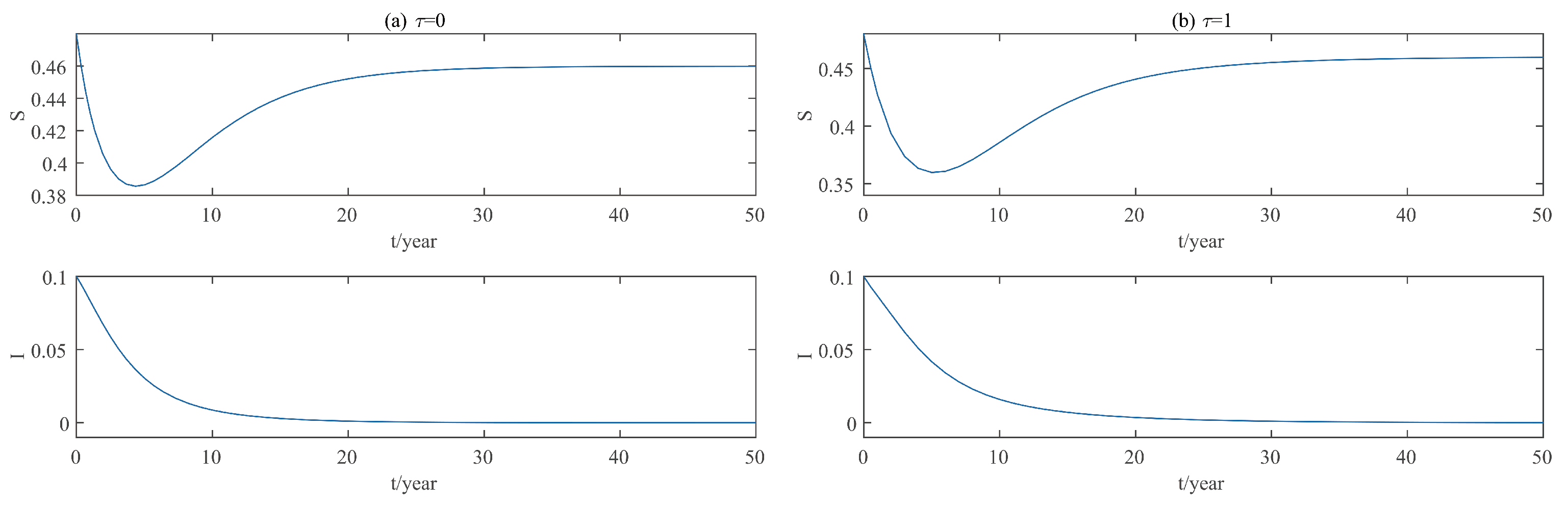
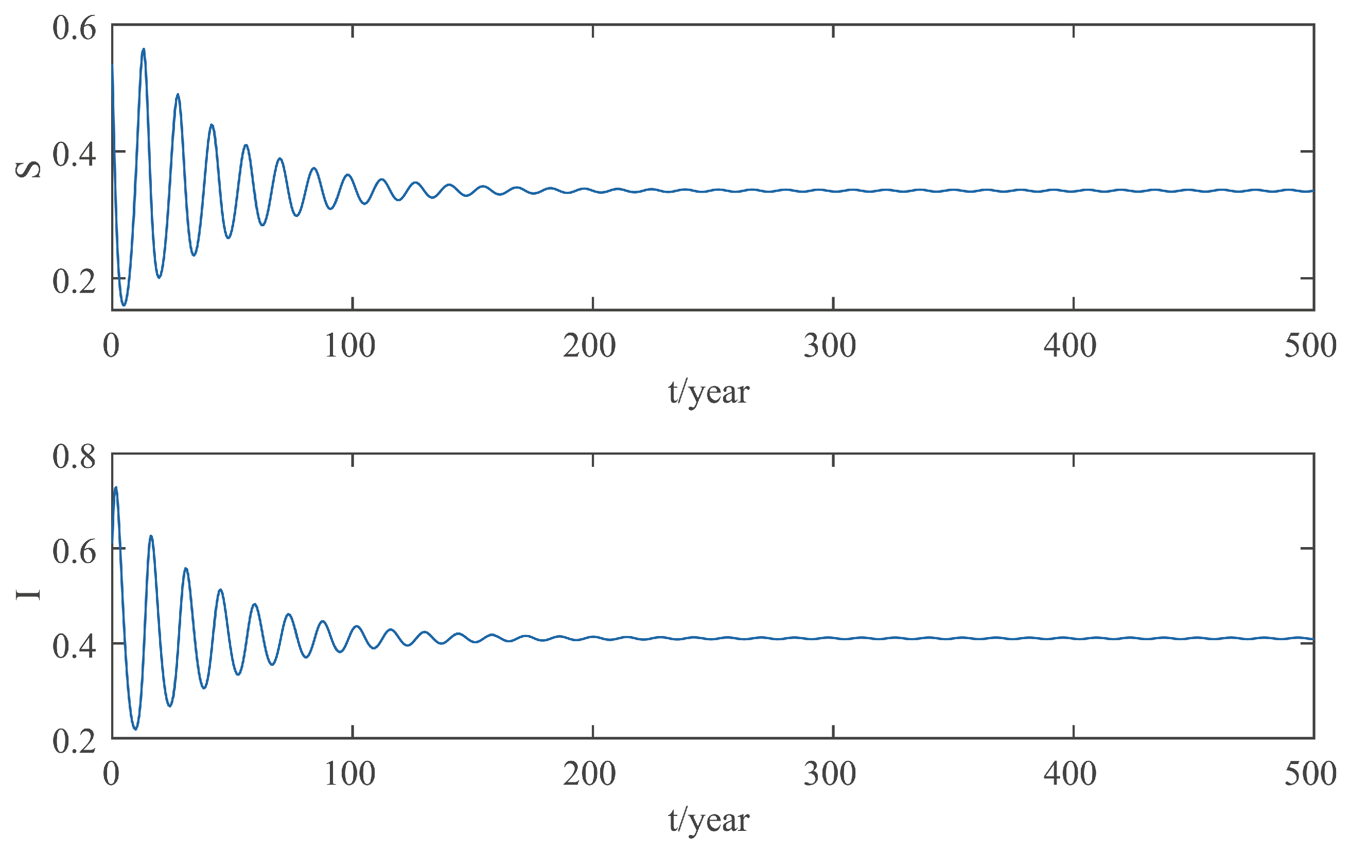
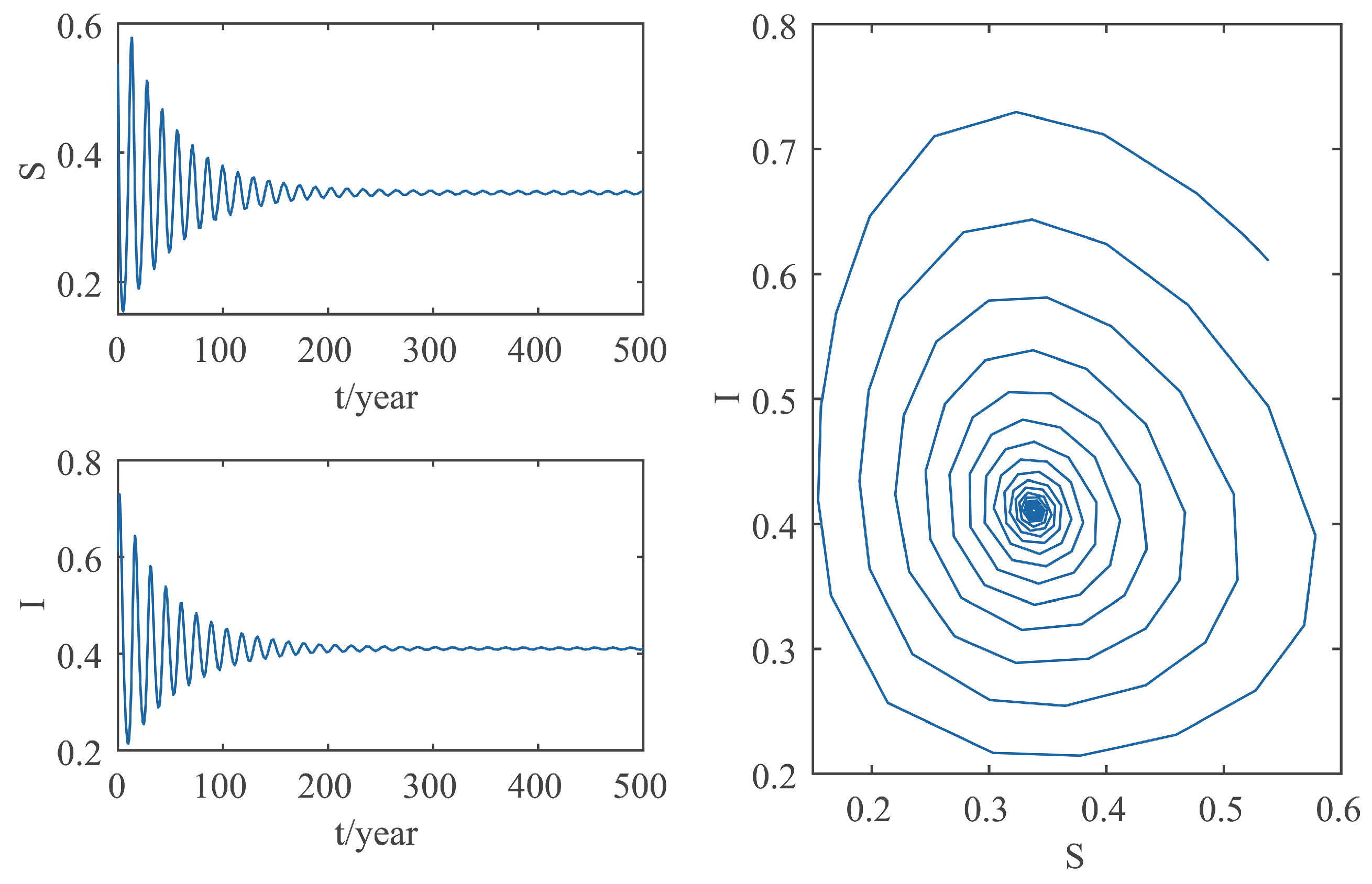
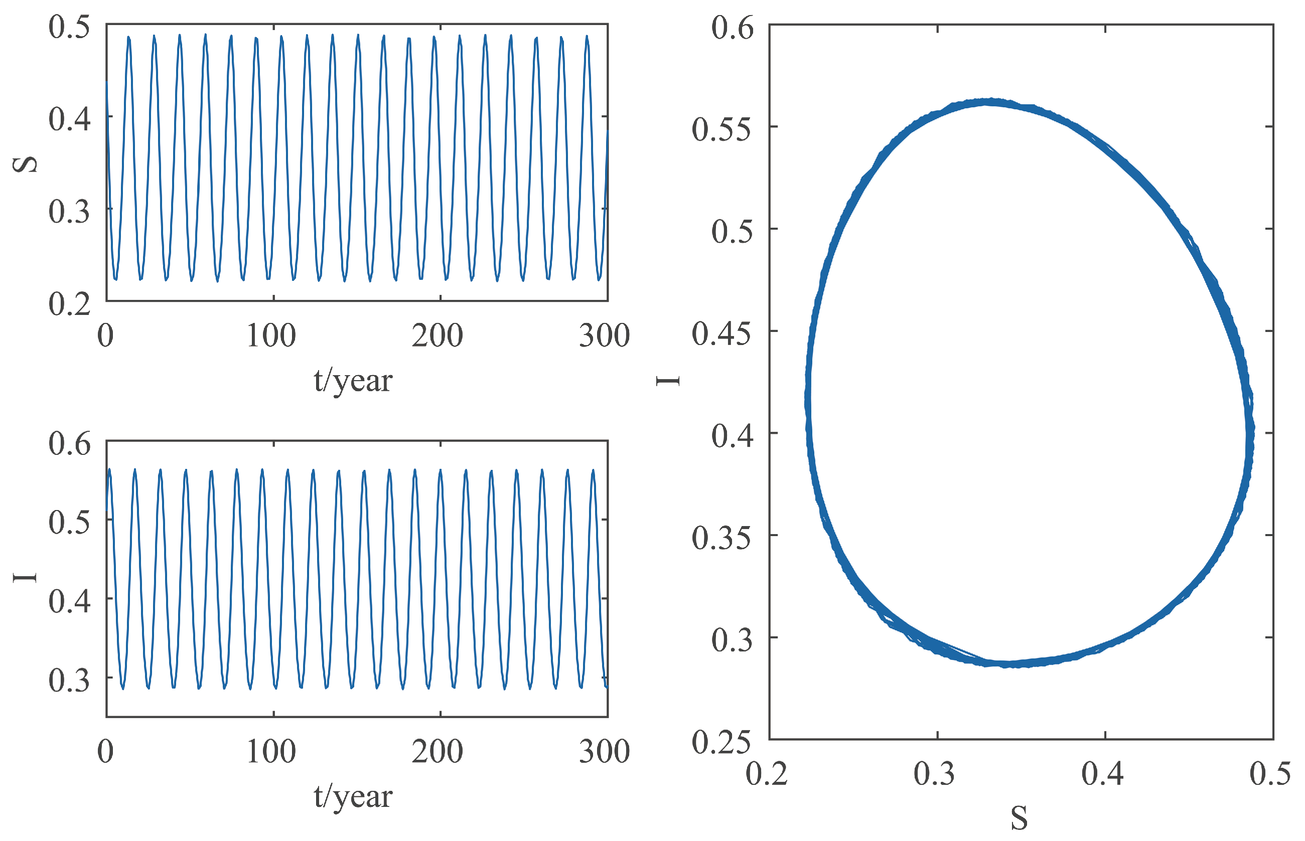
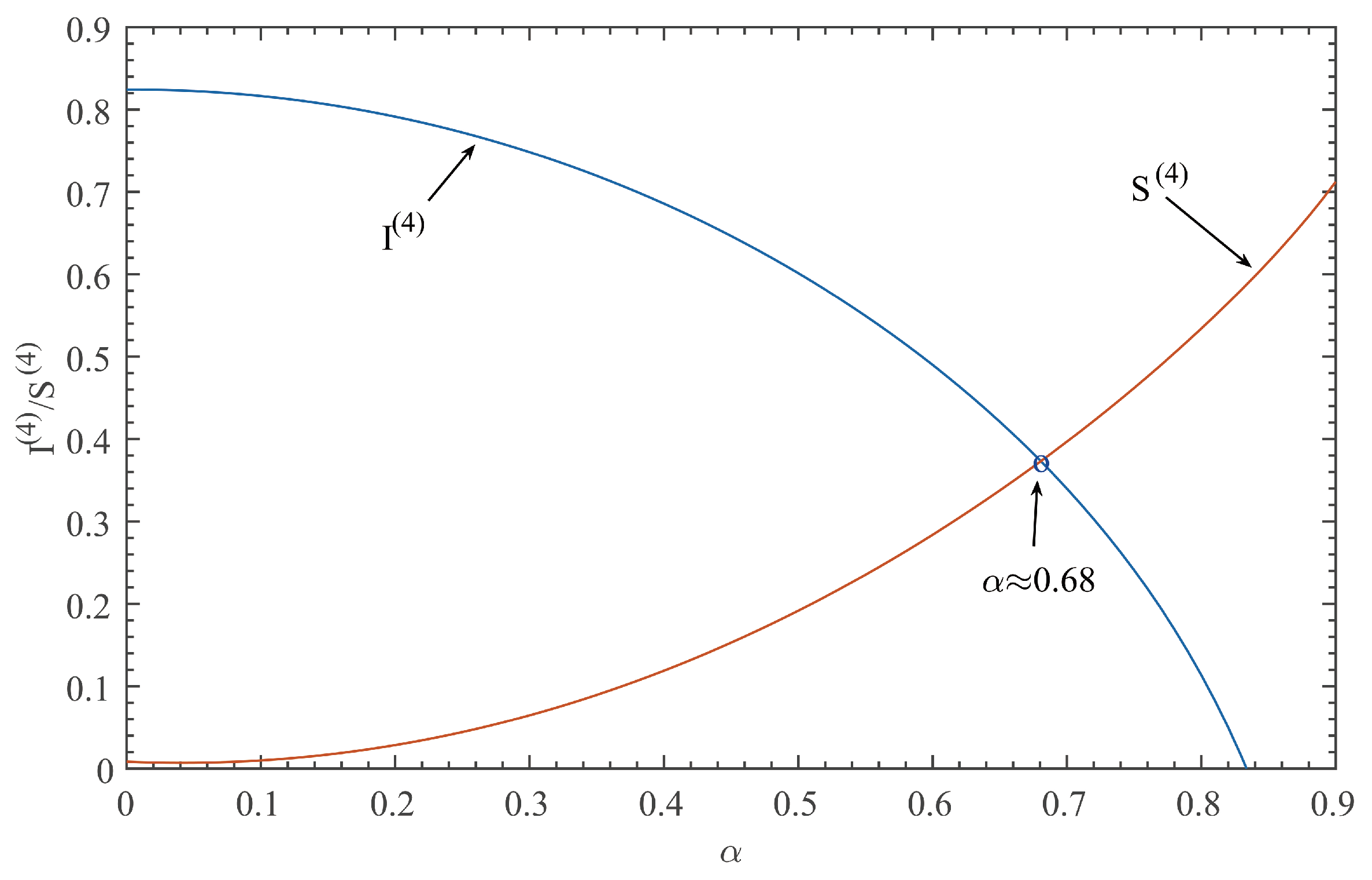
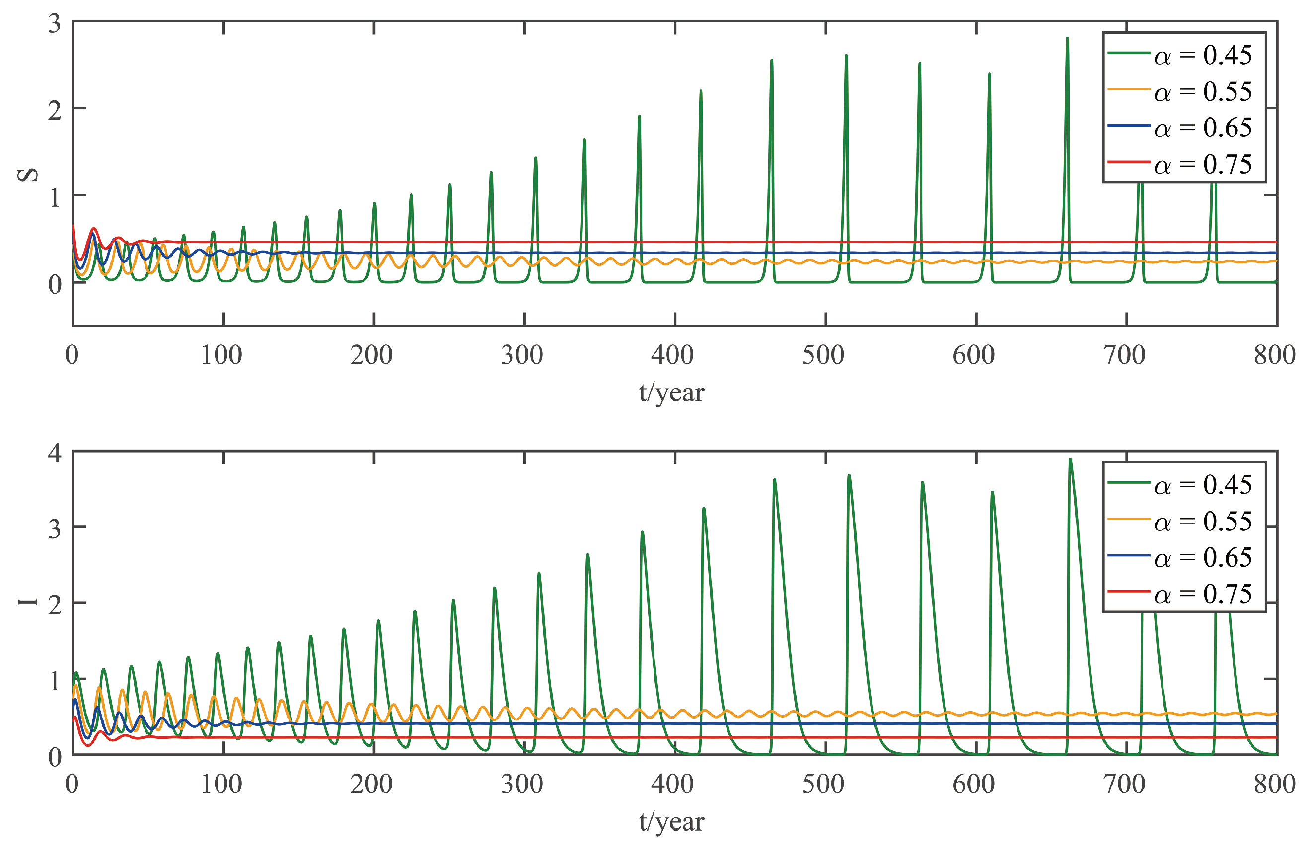
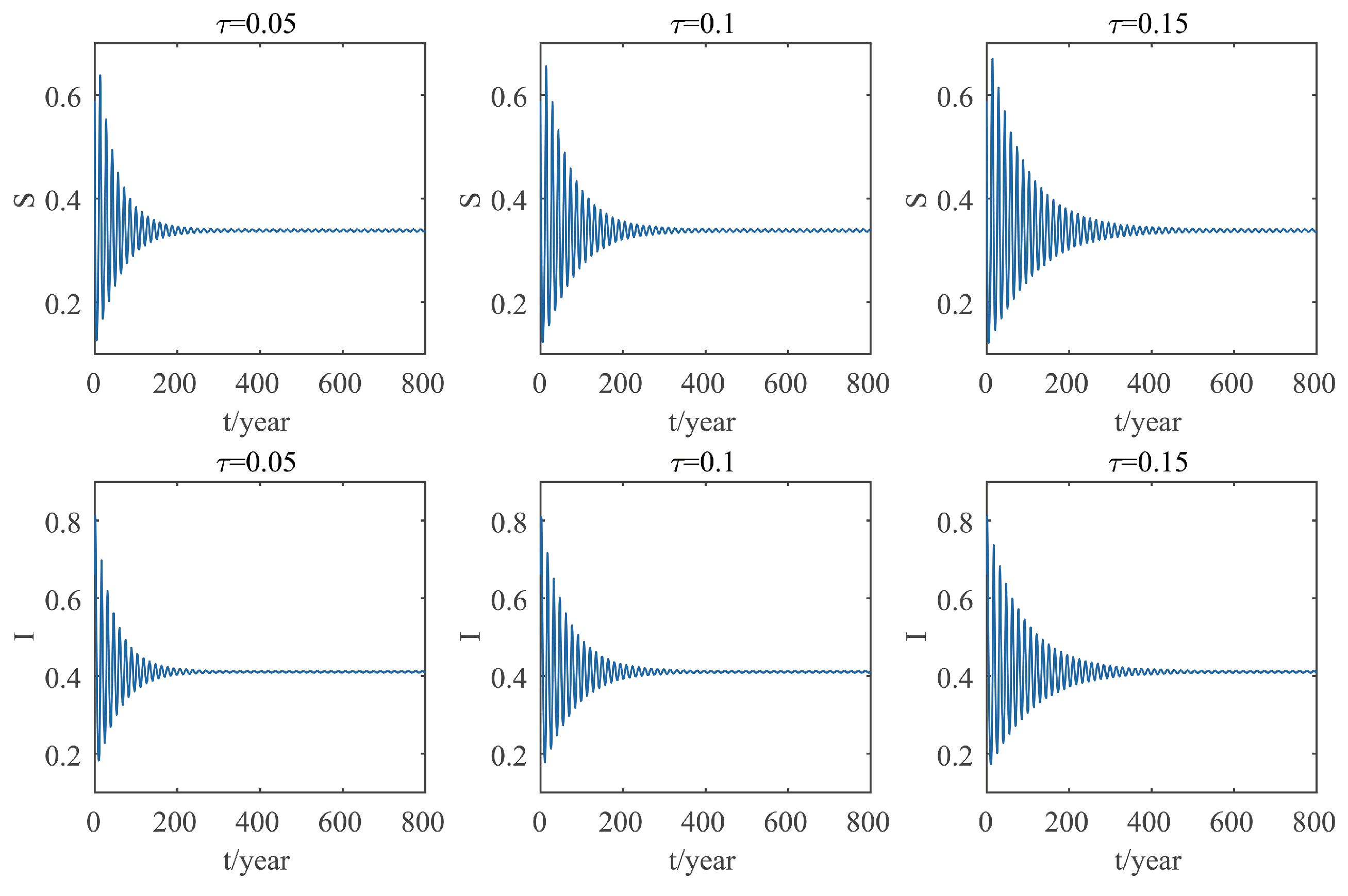
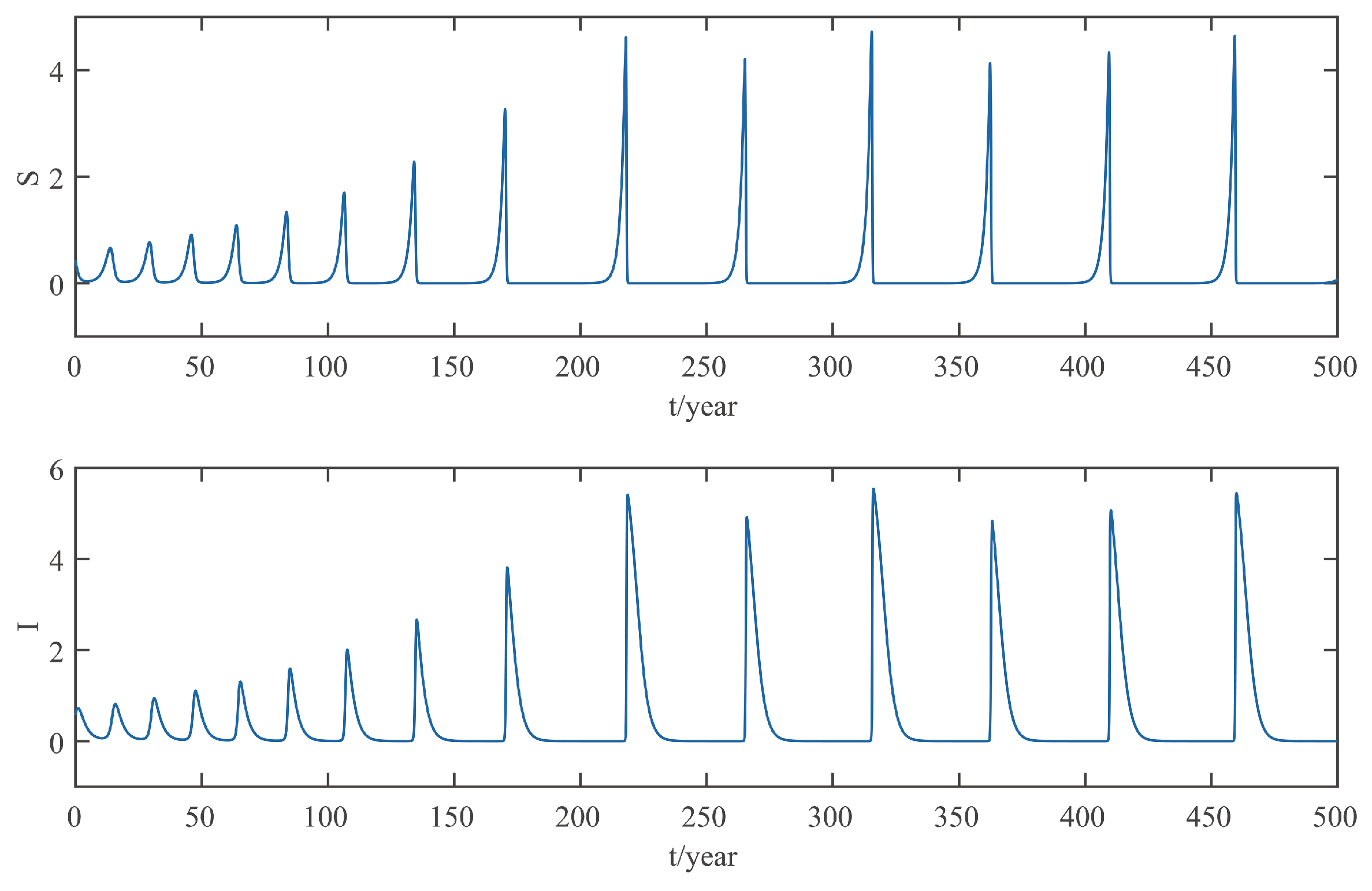
This paper focuses on the dynamics of the insect-vector populations based on SI epidemic model. By dividing M. alternatus into susceptible and infected, we have constructed a two-dimensional delay differential equation model considering the control intensity and the time delay for control to take effect. After that, we have analyzed the existence and stability of the equilibrium and the existence of Hopf bifurcation, and derived the normal form of Hopf bifurcation by using a multiple time scales method. Finally, by selecting scientific parameters for numerical simulation, the results of our theoretical analysis have been verified. Numerical analysis shows that when the intensity of control is large (obviously, if the intensity of control is large, then the environmental carrying capacity of M. alternatus will decrease accordingly), the disease-free equilibrium $E_3$ is always stable; when the intensity of control is 55%∼75%, the disease-free equilibrium $E_3$ is unstable for any $\tau \ge 0$, and oppositely, the positive equilibrium $E_4$ is stable before the critical time delay ${\tau }_1^{\left(0\right)}$, and the system will occur stable Hopf bifurcation periodic solution near equilibrium $E_4$. If the environmental carrying capacity of M. alternatus is large, the disease-free equilibrium $E_3$ does not exist and the positive equilibrium $E_4$ cannot reach stability, which provides a theoretical support for the prevention and control of PWD. However, in fact, there are many difficulties in the disease control. For example, the effect of control is affected by many factors, so it is unrealistic for the intensity of disease control $\alpha$ to remain constant. In the process of modeling, we assume that the parameters are constant; in reality, the parameters are changing over time. However, in general, the stability of our model is consistent with the reality. Based on the stability analysis, more effective measures can be taken to reduce the damage caused by PWD.

In addition, our numerical analysis also shows that the number of infected M. alternatus decreases with the control intensity increasing, and the time for the system to reach stability increases with the time delay increasing. Therefore, it is important to increase the control intensity and shorten the time delay of control to take effect. Here, we suggest that in the process of prevention and control, we can choose combined measures to increase control intensity. Meanwhile, we suggest strengthening the monitoring of trees to take measures on trees as soon as possible to shorten the time delay. Moreover, when the the system eventually fails to reach stability, the disease outbreak shows apparent periodicity. In this way, we can better prevent the outbreak of PWD according to some rules, which can prolong the growth cycle of trees and reduce the loss of forest resources, and thus, improve the carbon sink capacity of forests and accelerate the realization of the goal of “emission peak and carbon neutrality”, so as to build a modernized country in which humanity and nature coexist in harmony.

References

1. Boone, C.K.; Sweeney, J.; Silk, P.; Hughes, C.; Webster, R.P.; Stephen, F.; Maclauchlan, L.; Bentz, B.; Drumont, A.; Zhao, B.; et al. Monochamus species from different continents can be effectively detected with the same trapping protocol. J. Pest Sci. 2018, 92, 3–11. [Google Scholar] [CrossRef]
2. Futai, K. Pine Wood Nematode, Bursaphelenchus xylophilus. Annu. Rev. Phytopathol. 2013, 51, 61–83. [Google Scholar] [CrossRef]
3. Mamiya, Y. History of pine wilt disease in Japan. J. Nematol. 1988, 20, 26–219. [Google Scholar]
4. Han, H.; Chung, Y.J.; Shin, S.C. First report of pine wilt disease on Pinus koraiensis in Korea. Plant Dis. 2008, 92, 1251. [Google Scholar] [CrossRef]
5. Zhao, B.G. Pine wilt disease in China. In Pine Wilt Disease; Springer: Tokyo, Japan, 2008; pp. 18–25. [Google Scholar]
6. Dwinell, L.D. First report of pinewood nematode (Bursaphelenchus xylophilus) in Mexico. Plant Dis. 1993, 77, 846. [Google Scholar] [CrossRef]
7. Abelleira, A.; Picoaga, A.; Mansilla, J.P.; Aguin, O. Detection of Bursaphelenchus xylophilus, causal agent of pine wilt disease on Pinus pinaster in Northwestern Spain. Plant Dis. 2011, 95, 776. [Google Scholar] [CrossRef]
8. Kim, S.H.; Yun, H.Y.; Jeong, H.J. Generation of a novel antibody against BxPrx, a diagnostic marker of pine wilt disease. Mol. Biol. Rep. 2023, 50, 4715–4721. [Google Scholar] [CrossRef] [PubMed]
9. Ding, X.; Ye, J.; Wu, X.; Huang, L.; Zhu, L.; Lin, S. Deep sequencing analyses of pine wood nematode Bursaphelenchus xylophilus microRNAs reveal distinct miRNA expression patterns during the pathological process of pine wilt disease. Gene 2015, 555, 346–356. [Google Scholar] [CrossRef]
10. Palomares-Rius, J.E.; Tsai, I.J.; Karim, N.; Akiba, M.; Kato, T.; Maruyama, H.; Takeuchi, Y.; Kikuchi, T. Genome-wide variation in the pinewood nematode Bursaphelenchus xylophilus and its relationship with pathogenic traits. BMC Genom. 2015, 16, 1–13. [Google Scholar] [CrossRef]
11. Wang, G.; Xu, X.; Cheng, Q.; Hu, J.; Xu, X.; Zhang, Y.; Guo, S.; Ji, Y.; Zhou, C.; Gao, F.; et al. Preparation of sustainable release mesoporous silica nano-pesticide for control of Monochamus alternatus. Sustain. Mater. Technol. 2023, 35, e00538. [Google Scholar] [CrossRef]
12. Lee, J.W.; Mwamula, A.O.; Choi, J.H.; Lee, H.W.; Kim, Y.S.; Kim, J.H.; Choi, Y.H.; Lee, D.W. Comparative bioactivity of emamectin benzoate formulations against the pine wood nematode, Bursaphelenchus xylophilus. Plant Pathol. J. 2023, 39, 75–87. [Google Scholar] [CrossRef] [PubMed]
13. Alvarez, G.; Etxebeste, I.; Gallego, D.; David, G.; Bonifacio, L.; Jactel, H.; Sousa, E.; Pajares, J.A. Optimization of traps for live trapping of Pine Wood Nematode vector Monochamus galloprovincialis. J. Appl. Entomol. 2015, 139, 618–626. [Google Scholar] [CrossRef]
14. Mannaa, M.; Han, G.; Jeon, H.W.; Kim, J.; Kim, N.; Park, A.R.; Kim, J.C.; Seo, Y.S. Influence of resistance-inducing chemical elicitors against pine wilt disease on the rhizosphere microbiome. Microorganisms 2020, 8, 884. [Google Scholar] [CrossRef]
15. Shi, X.Y.; Song, G.H. Analysis of the mathematical model for the spread of pine wilt disease. J. Appl. Math. 2013, 184054, 227–261. [Google Scholar] [CrossRef]
16. Ozair, M. Analysis of pine wilt disease model with nonlinear incidence and horizontal transmission. J. Appl. Math. 2014, 204241, 1–9. [Google Scholar] [CrossRef]
17. Khan, M.A.; Ali, K.; Bonyah, E.; Okosun, K.O.; Islam, S.; Khan, A. Mathematical modeling and stability analysis of pine wilt disease with optimal control. Sci. Rep. 2017, 7, 3115. [Google Scholar] [CrossRef]
18. Khan, M.A.; Ahmed, L.; Mandal, P.K.; Smith, R.; Haque, M. Modelling the dynamics of pine wilt disease with asymptomatic carriers and optimal control. Sci. Rep. 2020, 10, 11412. [Google Scholar] [CrossRef] [PubMed]
19. Nayfeh, A.H. Introduction to Perturbation Techniques; Wiley-Interscience: New York, NY, USA, 1981. [Google Scholar]
20. Nayfeh, A.H. Order reduction of retarded nonlinear systems—The method of multiple scales versus center-manifold reduction. Nonlinear Dyn. 2008, 51, 483–500. [Google Scholar] [CrossRef]
21. Ding, Y.T.; Zheng, L.Y. Mathematical modeling and dynamics analysis of delayed nonlinear VOC emission system. Nonlinear Dyn. 2022, 109, 3157–3167. [Google Scholar] [CrossRef]
22. Shen, H.; Song, Y.L.; Wang, H. Bifurcations in a diffusive resource-consumer model with distributed memory. J. Differ. Equ. 2023, 347, 170–211. [Google Scholar] [CrossRef]
23. Liu, M.; Wang, H.B.; Jiang, W.H. Bifurcations and pattern formation in a predator-prey model with memory-based diffusion. J. Differ. Equ. 2023, 350, 1–40. [Google Scholar] [CrossRef]
24. Wang, Y.; Chen, J.; Chen, F.; Zhou, Q.; Zhou, L.; Sun, S. Transmission of Bursaphelenchus xylophilus (Nematoda: Aphelenchoididae) through feeding activity of Monochamus alternatus (Coleoptera: Cerambycidae). J. Nanjing For. Univ. 2019, 43, 1–10. [Google Scholar]
25. Jikumaru, S.; Togashi, K. Temperature Effects on the transmission of Bursaphelenchus xylophilus (Nemata: Aphelenchoididae) by Monochamus alternatus (Coleoptera: Cerambycidae). J. Nematol. 2000, 32, 110–116. [Google Scholar] [PubMed]
26. Koutroumpa, F.A.; Vincent, B.; Roux-Morabito, G.; Martin, C.; Lieutier, F. Fecundity and larval development of Monochamus galloprovincialis (Coleoptera Cerambycidae) in experimental breeding. Ann. For. Sci. 2008, 65, 707. [Google Scholar] [CrossRef]
27. Li, M.; Dai, Y.; Wang, Y.; Wang, L.; Sun, S.; Chen, F. New insights into the life history of Monochamus saltuarius (Cerambycidae: Coleoptera) can enhance surveillance strategies for pine wilt disease. J. For. Res. 2021, 32, 2699–2707. [Google Scholar] [CrossRef]
28. Ahmed, E.S.; Rida, S.Z.; Gaber, Y.A. On the stability analysis and solutions of fractional order pine wilt disease model. Appl. Math. Inf. Sci. 2020, 14, 1137–1146. [Google Scholar]
29. Zhao, L.; Sun, J. Pinewood Nematode Bursaphelenchus xylophilus (Steiner and Buhrer) Nickle; Springer: Singapore, 2017; Volume 13, pp. 3–21. [Google Scholar]
Figure 1. Variable relation of the infection-control system.
Mathematics 11 03705 g001
Figure 2. Relationship curve between longevity of M. alternatus and amount of PWN carried.
Mathematics 11 03705 g002
Figure 3. Equilibrium E 3 of system (2) is locally asymptotically stable.
Mathematics 11 03705 g003
Figure 4. Equilibrium E 4 of system (2) for τ = 0 is locally asymptotically stable.
Mathematics 11 03705 g004
Figure 5. Equilibrium E 4 of system (2) for τ = 0.05 is locally asymptotically stable.
Mathematics 11 03705 g005
Figure 6. System (2) for τ = 0.30245 occurs stable and forward Hopf bifurcation periodic solution near equilibrium E 4 .
Mathematics 11 03705 g006
Figure 7. Dynamic curve of the equilibrium E 4 with the intensity of artificial control α .
Mathematics 11 03705 g007
Figure 8. Comparison of convergence speed of S and I for τ = 0 under different α .
Mathematics 11 03705 g008
Figure 9. Comparison of convergence speed of S and I for α = 0.65 under different τ .
Mathematics 11 03705 g009
Figure 10. Equilibrium E 4 of system (2) for τ = 0 is unstable.
Mathematics 11 03705 g010