Physics-Informed Neural Networks and Functional Interpolation for Solving the Matrix Differential Riccati Equation

Abstract

In this manuscript, we explore how the solution of the matrix differential Riccati equation (MDRE) can be computed with the Extreme Theory of Functional Connections (X-TFC). X-TFC is a physics-informed neural network that uses functional interpolation to analytically satisfy linear constraints, such as the MDRE’s terminal constraint. We utilize two approaches for solving the MDRE with X-TFC: direct and indirect implementation. The first approach involves solving the MDRE directly with X-TFC, where the matrix equations are vectorized to form a system of first order differential equations and solved with iterative least squares. In the latter approach, the MDRE is first transformed into a matrix differential Lyapunov equation (MDLE) based on the anti-stabilizing solution of the algebraic Riccati equation. The MDLE is easier to solve with X-TFC because it is linear, while the MDRE is nonlinear. Furthermore, the MDLE solution can easily be transformed back into the MDRE solution. Both approaches are validated by solving a fluid catalytic reactor problem and comparing the results with several state-of-the-art methods. Our work demonstrates that the first approach should be performed if a highly accurate solution is desired, while the second approach should be used if a quicker computation time is needed.

1. Introduction

In 1960, Rudolph E. Kalman introduced a paper that was the first to describe how the solution of the matrix differential Riccati equation (MDRE) can be used to compute the state feedback gain of the optimal controller for a general linear system with a quadratic performance criterion [1]. Over time, Kalman’s discovery proved to be groundbreaking and is still very relevant today. An optimal controller derived from the MDRE’s solution is called a linear–quadratic regulator (LQR), and is used throughout academia and industry to solve a wide array of engineering problems. Nearly every course on control algorithms teaches the fundamental notions of LQR controllers. Unfortunately, the MDRE rarely possesses an analytical solution but can almost always be computed numerically. Motivated to find more accurate and quicker solutions, researchers have proposed many robust numerical techniques for acquiring the MDRE’s solution since 1960. In the same vein as researchers of the past, this manuscript also explores new ways of solving the MDRE. The novelty of our work comes from our use of a new physics-informed neural network (PINN)-based framework to solve the MDRE, called the Extreme Theory of Function Connections (X-TFC) [2].

1.1. Related Work

The MDRE arising from a linear–quadratic optimal control problem rarely, if ever, possesses an analytical solution. Thus, many numerical techniques for acquiring the MDRE solution have been proposed. Perhaps the simplest way to solve an MDRE numerically is with a direct integration procedure (e.g., Runge–Kutta or Euler routines). However, this approach can be relatively slow for large systems and does not always yield accurate results, especially when the system is stiff [3,4]. Several alternatives to direct integration involve transforming the MDRE into an equivalent linear differential Hamiltonian system: the Kalman–Englar method (the Kalman–Englar method is also referred to as the automatic synthesis program (ASP) matrix iteration procedure in other works [3,5]) [6], the Davison–Maki algorithm [7], the Vaughan negative exponential technique [8], and a Schur approach [9]. Each of these procedures obtains the solution of the MDRE by partitioning the transition matrix of the associated Hamiltonian system in their own unique way. The Chandrasekhar method [10] instead transforms the MDRE into a different system of nonlinear differential equations (DEs), but with lesser dimensionality. This method is particularly efficient when the number of controllers and observers is small [5].

One can use the solution of the matrix algebraic Riccati equation (MARE) to obtain the infinite-horizon optimal control law if the linear system is time-invariant. However, reducing the MDRE to an MARE when the linear–quadratic optimal control problem has finite final time will cause the control algorithm to lose its optimality and induce significant control inefficiency. Nevertheless, researchers still found ways to employ the MARE to solve the MDRE. For example, Anderson and Moore found the MDRE solution by transforming the MDRE into a matrix differential Lyapunov equation (MDLE) based on the positive definite solution of the MARE [11]. Commonly referred to as the Anderson–Moore method in the literature (although Anderson and Moore have received much of the credit for coming up with the idea to solve the MDRE based on transforming it into an MDLE based on the MARE, the authors of this work recognize that Potter came up with a very similar method first [12,13]), this method is advantageous because it requires a smaller amount of computation than others. Conversely, its applicability is narrower than other methods because it requires stringent invertible conditions. Two studies have been carried out to improve the Anderson–Moore method by enforcing milder assumptions. The technique proposed by Radisavljevic transforms the MDLE into a Hamiltonian system containing algebraic Lyapunov equations [14]. Solutions of the Hamiltonian system are found in terms of state transition matrices, and clever matrix algebra is used to avoid singular inversions. Alternatively, the Nguyen and Gajic method transforms the MDRE into an MDLE based on the negative definite solution of the MARE [15]. Thus, the invertible conditions from the Anderson–Moore method are replaced with positive semi-definite conditions, which are easier to deal with.

Researchers in the machine learning community have even explored solving the MDRE. For example, Balasubramaniam et al. solved the MDRE by approximating its solution with a neural network [16]. They composed the loss function in their algorithm as the difference between the derivative of their approximation and the right-hand side of the MDRE with their approximation substituted in. In other words, the authors used the residual of the MDRE as the loss function. Following the work of Reference [16], more complex MDREs from singular, stochastic, and fuzzy systems were quickly solved [17,18,19,20,21]. Each neural network in these studies was trained with the Levenberg–Marquardt algorithm and validated by comparisons with the Runge–Kutta algorithm. This manuscript also uses neural networks to solve the MDRE and compares them with the Runge–Kutta algorithm, but we use a different optimization scheme.

1.2. Contributions and Scope of This Work

Our goal is to improve upon how neural networks can be used to solve the MDRE. For example, we explicitly state our use of PINNs, which are a class of machine learning algorithms that have recently been used to solve a plethora of DEs [22,23]. They are better at solving such problems than standard neural networks because they incorporate the DE residuals into the loss function (i.e., taking into account physical laws), allowing the solution to be found in a data-physics-driven manner. PINNs can even find the solutions of DEs in a purely physics-driven fashion when no data are available. When the neural network is fully trained, an analytical representation of the solution is achieved. Indeed, the aforementioned works that used neural networks to solve the MDRE can be classified as PINNs, although the authors do not explicitly state their use. In this work, we use a PINN-based framework called X-TFC to solve the MDRE.

X-TFC is a novel and efficient PINN model that merges neural networks and the Theory of Functional Connections (TFC) [24]. TFC is a functional interpolation framework that finds all possible functions satisfying given linear constraints. It has the potential to be used for many mathematical problems, but it has been heavily used for computing the solution of DEs. This is because it can analytically embed the constraints of a particular DE into a closed-form approximation of the solution, called constrained expressions. Exploiting this trait has allowed TFC to solve a plethora of DEs with machine-level accuracy and in milliseconds [25,26]. TFC’s constrained expressions are functionals made up of an arbitrary free function, and the sum of switching and projection function products. Essentially, the summation terms handle the constraint embedding, while the unknowns within the free function are optimized to minimize the residual of the DE. In the original formulation of TFC, a truncated expansion of orthogonal polynomials was selected as the free function. Using such free functions proved troublesome when solving large-scale partial DEs due to the curse of dimensionality. X-TFC was developed to overcome this limitation by utilizing a single-layer feedforward neural network (SLFNN), trained via the Extreme Learning Machine (ELM) algorithm [27], as the free function. The inclusion of an SLFNN and the DE residual in a loss function is what allows X-TFC to be considered as a PINN-based framework. Eventually, it was shown that X-TFC is competitive with TFC when solving ordinary DEs as well. As a matter of fact, it has already been used to solve several problems related to optimal control [28,29], which contributed to the motivation of this work.

We use X-TFC to solve the MDRE in two distinct ways: directly and indirectly by solving the MDLE from Reference [15]. The first approach we employ involves solving the MDRE directly with X-TFC, where the matrix equations are vectorized to form a system of first order DEs. Note that the solution of the MDRE is generally referred to as the Riccati matrix, and by assuming it is symmetric, only its upper triangular elements must be approximated. Furthermore, the domain of the DEs can be decomposed to provide a more accurate approximation of the solution. As described in Reference [15], an alternative technique is to first transform the MDRE into the MDLE based on the anti-stabilizing solution of the MARE. The MDLE’s solution can then be transformed back into the MDRE’s solution. Thus, we also explore solving the MDRE indirectly by first solving the MDLE with X-TFC. Whether solving the MDRE or MDLE, doing so with X-TFC is an improvement over standard PINNs because the terminal constraint is satisfied exactly with functional interpolation and X-TFC’s optimization scheme uses least squares, which is much quicker than those involving learning rates, such as the Levenberg–Marquardt algorithm. Lastly, one more important contribution of this study is that it is the first X-TFC work to investigate initializing the input weights and biases of the SLFNN with a deterministic sequence.

The remaining content of this manuscript is organized as follows. In the forthcoming section, the MDRE and MDLE are clearly defined. Afterwards, the X-TFC method is introduced to solve both equations. A theorem that gives the maximum bound of X-TFC’s generalization error is also given. Next, we present numerical experiments that demonstrate X-TFC’s ability to acquire the MDRE solution directly and indirectly by solving the MDLE. We also provide comparisons with the Runge–Kutta 4 (RK4) method of direct integration and the Lyapunov approach from Nguyen and Gajic (NG) [15], where the Kalman–Englar (KE) method is used as a benchmark. The results are discussed in detail. Lastly, the paper is concluded with final thoughts and the outlook for further research.

2. Problem Statement

Consider the linear time-invariant system

$$\dot{\mathit{x}}\left(t\right)=\mathit{A}\mathit{x}\left(t\right)+\mathit{B}\mathit{u}\left(t\right);\mathit{x}\left(t_0\right)={\mathit{x}}_0,$$

(1)

where $\mathit{x}\left(t\right)$ is an n dimensional state vector, $\mathit{A}$ is an $n\times n$ matrix, $\mathit{u}\left(t\right)$ is an m dimensional control input vector, and $\mathit{B}$ is an $n\times m$ matrix. Furthermore, the initial state is known as $\mathit{x}\left(t_0\right)={\mathit{x}}_0$. The goal of the optimal control problem associated with this system is to find the optimal control that minimizes the finite-horizon linear–quadratic cost functional

$$\mathcal{J}={\mathit{x}}^{⊺}\left(t_f\right)\mathit{S}\mathit{x}\left(t_f\right)+\frac{1}{2}{\int }_{t_0}^{t_f}\left({\mathit{x}}^{⊺}\left(t\right)\mathit{Q}\mathit{x}\left(t\right)+{\mathit{u}}^{⊺}\left(t\right)\mathit{R}\mathit{u}\left(t\right)\right)\mathrm{d}t,$$

(2)

where $\mathit{Q}\ge 0$, $\mathit{S}\ge 0$, and $\mathit{R}>0$ are constant matrices of appropriate dimensions. Furthermore, $t_0$ and $t_f$ are the initial and final time, respectively.

2.1. Matrix Differential Riccati Equation

One could solve the optimal control problem via Pontryagin’s Minimum Principle (PMP) [30], where the Hamiltonian $\mathcal{H}$ is derived and minimized to write the control in terms of the costate vector $\mathit{\lambda }\in {\mathbb{R}}^n$:

$$\begin{array}{cc}\hfill \mathcal{H}& =\frac{1}{2}\left({\mathit{x}}^{⊺}\mathit{Q}\mathit{x}+{\mathit{u}}^{⊺}\mathit{R}\mathit{u}\right)+{\mathit{\lambda }}^{⊺}\left(\mathit{A}\mathit{x}+\mathit{B}\mathit{u}\right)\hfill \\ \hfill \mathbf{0}& =\frac{\partial \mathcal{H}}{\partial \mathit{u}}=\mathit{R}\mathit{u}+{\mathit{B}}^{⊺}\mathit{\lambda }\to \mathit{u}=-{\mathit{R}}^{-1}{\mathit{B}}^{⊺}\mathit{\lambda }.\hfill \end{array}$$

(3)

The necessary conditions of optimality are then satisfied by solving the following two-point boundary value problem (TPBVP), considering also the corresponding boundary and transversality conditions:

$$\begin{array}{cc}\hfill \dot{\mathit{x}}& =\frac{\partial \mathcal{H}}{\partial \mathit{\lambda }}=\mathit{A}\mathit{x}+\mathit{B}\mathit{u};\mathit{x}\left(t_0\right)={\mathit{x}}_0\hfill \end{array}$$

(4a)

$$\begin{array}{cc}\hfill \dot{\mathit{\lambda }}& =-\frac{\partial \mathcal{H}}{\partial \mathit{x}}=-\mathit{Q}\mathit{x}-{\mathit{A}}^{⊺}\mathit{\lambda };\mathit{\lambda }\left(t_f\right)=\mathit{S}\mathit{x}\left(t_f\right).\hfill \end{array}$$

(4b)

Note that the solution of the above TPBVP is also sufficiently optimal because of the strengthened Legendre–Clebsch condition (i.e., ${\mathcal{H}}_{\mathit{u}\mathit{u}}>0$). Instead of solving the TPBVP, one can guess the form of the solution to be

$$\mathit{\lambda }\left(t\right)=\mathit{P}\left(t\right)\mathit{x}\left(t\right),$$

(5)

which when plugged into Equation (4b) gives

$$\begin{array}{cc}\hfill \dot{\mathit{\lambda }}& =\dot{\mathit{P}}\mathit{x}+\mathit{P}\dot{\mathit{x}}\hfill \\ \hfill & =\dot{\mathit{P}}\mathit{x}+\mathit{P}\left(\mathit{A}-\mathit{B}{\mathit{R}}^{-1}{\mathit{B}}^{⊺}\mathit{P}\right)\mathit{x}\hfill \\ & =\dot{\mathit{P}}\mathit{x}+\mathit{P}\mathit{A}\mathit{x}-\mathit{P}\mathit{B}{\mathit{R}}^{-1}{\mathit{B}}^{⊺}\mathit{P}\mathit{x}=-\mathit{Q}\mathit{x}-{\mathit{A}}^{⊺}\mathit{P}\mathit{x}.\hfill \end{array}$$

(6)

Simplifying the above equation yields the MDRE,

$$-\dot{\mathit{P}}=\mathit{P}\mathit{A}+{\mathit{A}}^{⊺}\mathit{P}-\mathit{P}\mathit{G}\mathit{P}+\mathit{Q};\mathit{P}\left(t_f\right)=\mathit{S},$$

(7)

where

$$\mathit{G}=\mathit{B}{\mathit{R}}^{-1}{\mathit{B}}^{⊺}.$$

(8)

The matrix $\mathit{P}\left(t\right)\in {\mathbb{R}}^{n\times n}$ in the above derivation is known as the Riccati matrix and is the solution to the MDRE. The MDRE is a system of ordinary DEs with a terminal constraint that can be solved backwards in time. When solved, the closed-loop solution of the optimal control problem can then be determined as

$$\mathit{u}\left(t\right)={\mathit{R}}^{-1}{\mathit{B}}^{⊺}\mathit{P}\left(t\right)\mathit{x}\left(t\right).$$

(9)

2.2. Matrix Differential Lyapunov Equation

Instead of directly computing the solution of the MDRE, several researchers sought to find the inverse of the difference between the MDRE solution $\mathit{P}$ and the positive definite solution of the MARE ${\mathit{P}}^{+}$. However, this is problematic when the difference is near singular. Furthermore, a crucial requirement when ${\mathit{P}}^{+}$ is exploited is that $\mathit{P}\mathit{S}-{\mathit{P}}^{+}$ must be invertible. Nguyen and Gajic showed that utilizing the negative definite solution of the MARE ${\mathit{P}}^{-}$, instead of ${\mathit{P}}^{+}$, reduces the invertibility requirement to simply $\mathit{S}\ge 0$ [15]. Here we merely provide a general outline of Nguyen and Gajic’s method, which culminated in finding the solution of an MDLE based on ${\mathit{P}}^{-}$. For a more in-depth look at the assumptions, lemmas, and proofs that reveal how and why the solution of the MDLE based on the negative definite solution of the MARE solves the MDRE, we redirect the reader to Reference [15].

The MARE is given below,

$$\mathbf{0}=\mathit{P}\mathit{A}+{\mathit{A}}^{⊺}\mathit{P}-\mathit{P}\mathit{G}\mathit{P}+\mathit{Q},$$

(10)

where ${\mathit{P}}^{+}$ and ${\mathit{P}}^{-}$ are guaranteed to exist if $(\mathit{A},\mathit{B})$ is completely controllable and $(\mathit{A},\mathit{Q})$ is completely observable. ${\mathit{P}}^{-}$ can be found by solving the algebraic equation

$$\mathbf{0}=-{\mathit{P}}_n\mathit{A}-{\mathit{A}}^{⊺}{\mathit{P}}_n-{\mathit{P}}_n\mathit{G}{\mathit{P}}_n+\mathit{Q}$$

(11)

for its positive definite solution ${\mathit{P}}_n$. It can easily be shown that ${\mathit{P}}_n=-{\mathit{P}}^{-}$ is a positive definite solution of Equation (11). Subtracting Equation (10), with $\mathit{P}$ replaced by ${\mathit{P}}^{-}$, from Equation (7) gives the equation

$$\begin{array}{cc}\hfill -\dot{\mathit{P}}\left(t\right)& =(\mathit{P}\left(t\right)-{\mathit{P}}^{-})\mathit{A}+{\mathit{A}}^{⊺}(\mathit{P}\left(t\right)-{\mathit{P}}^{-})-\mathit{P}\left(t\right)\mathit{G}\mathit{P}\left(t\right)+{\mathit{P}}^{-}\mathit{G}{\mathit{P}}^{-}.\hfill \end{array}$$

(12)

By introducing the change in variable

$${\mathit{P}}_0\left(t\right)={\left(\mathit{P}\left(t\right)-{\mathit{P}}^{-}\right)}^{-1}$$

(13)

and enforcing the terminal condition from the MDRE, Equation (12) becomes

$$\begin{array}{cc}\hfill {\dot{\mathit{P}}}_0& ={\mathit{A}}_0{\mathit{P}}_0\left(t\right)+{\mathit{P}}_0\left(t\right){\mathit{A}}_0^{⊺}-\mathit{G};\hfill \\ \hfill & {\mathit{P}}_0\left(t_f\right)={\mathit{S}}_0={\left(\mathit{S}-{\mathit{P}}^{-}\right)}^{-1},\hfill \end{array}$$

(14)

where

$${\mathit{A}}_0=\mathit{A}-\mathit{G}{\mathit{P}}^{-}.$$

(15)

It can be seen that real eigenvalues of ${\mathit{A}}_0$ are greater than zero and Equation (14) is an MDLE. In addition, the MDLE is easier to solve than the MDRE because it is linear. Nguyen and Gajic went on to solve the MDLE by using techniques from References [31,32], which involve using the solution of a matrix algebraic Lyapunov equation and matrix exponentials. Here, we solve the MDLE with X-TFC. The solution of the MDRE can then be obtained as

$$\mathit{P}\left(t\right)=\left({\mathit{P}}^{-}+{\mathit{P}}_0^{-1}\left(t\right)\right).$$

(16)

3. Method

How the PINN and X-TFC methods are used to solve DEs, whether ordinary (ODE) or partial (PDE), has been well-documented [2,22,23]. The main differences between regular PINNs and X-TFC are that X-TFC analytically satisfies constraints with X-TFC and uses the ELM algorithm to train the network. Furthermore, in this work, X-TFC is purely physics-based. Only the ODE residuals are used in the loss function. PINNs and X-TFC have already been compared for solving two-point boundary value problems [28]. The logic can easily be continued for initial or final value problems (IVPs or FVPs). Likewise, De Florio et al. demonstrated how X-TFC can be used to solve a general ODE with one Dirichlet/point constraint [33]. These works outline the general X-TFC process:

• Write the ODE as a residual.
• Build the constrained expression approximation for the dependent variable in the ODE. Use a single-layer feedforward neural network with randomized input weights and biases (ELM expansion) as the free function.
• Plug the constrained expression into the residual and discretize the domain to form an unconstrained algebraic system of equations.
• Optimize for the unknowns in the free function that minimize the residual with iterative least squares if the problem is nonlinear or linear least squares if it is linear.

The most cumbersome part of the X-TFC process is building the constrained expression,

$$y_{\mathrm{ce}}(t,g\left(t\right))=g\left(t\right)+\sum _{i=1}^{N_{\mathrm{const}}}{\varphi }_i\left(t\right){\rho }_i(t,g\left(t\right)).$$

(17)

In Equation (17), $g\left(t\right)$ is the free function, ${\varphi }_i\left(t\right)$ are the switching functions, ${\rho }_i(t,g\left(t\right))$ are the projection functionals, and $N_{\mathrm{const}}$ is the number of linear constraints. The difficulty in building the constrained expression comes from deriving the switching functions via the selection of the projection functionals. This step is different for problems of varying constraints. Nonetheless, the correct switching functions and projection functionals to use for many constraints of many ODEs have already been published [34]. Moreover, deriving the switching functions for point constraints, such as the terminal constraints in the MDRE and MDLE, is very simple. Thus, in this work, we demonstrate how X-TFC can be used to solve the MDRE and the MDLE specifically. We leave the general formulation of the method to the aforestated works.

3.1. Solving Matrix Differential Riccati Equation with X-TFC

Although the MDRE is written in compact matrix form, it can be thought of as a system of first order ODEs. From here on, we adopt Einstein summation notation to show how X-TFC can be used to solve this system more clearly. Each time-varying element of the Riccati matrix can be written as $P_{ij}\left(t\right)\in {\mathbb{R}}^{n\times n}$ where the first and second indices (i and j in this case) represent the rows and columns of $\mathit{P}$, respectively. The rest of the matrices in Equation (7) are written in a similar manner. Thus, the MDRE in Einstein summation notation becomes

$$\begin{array}{cc}\hfill 0& ={\mathcal{R}}_{ij}={\dot{P}}_{ij}+P_{ik}{A}_{kj}+A_{ik}{P}_{jk}-P_{ik}{G}_{ko}{P}_{oj}+Q_{ij};\hfill \\ \hfill & P_{ij}\left(t_f\right)=S_{ij}.\hfill \end{array}$$

(18)

X-TFC is used to approximate $P_{ij}$ with constrained expressions containing SLFNNs and transform Equation (18) into an unconstrained optimization problem that can be solved with iterative least squares.

Since the MDRE only contains one constraint, the constrained expressions that we use to approximate the Riccati matrix elements are

$$P_{ij}\left(t\right)\approx g_{ij}\left(t\right)+\varphi \left(t\right){\rho }_{ij}(t_f,g_{ij}\left(t_f\right)).$$

(19)

Note that only one switching and projection function are present in Equation (19). The amount of $\varphi \left(t\right)\rho (t,g(t\left)\right)$ products in a constrained expression is equivalent to the amount of constraints on the DE. Hence, we require only one switching and projection function for each MDRE element because they are only constrained once at the end of the domain $t_f$. Conveniently, $\varphi \left(t\right)=1$ when there is only one constraint (see Reference [33]). Furthermore, the projection functional for point constraints is simply the difference between the constraint value and the free function,

$${\rho }_{ij}(t_f,g_{ij}\left(t_f\right))=P_{ij}\left(t_f\right)-g_{ij}\left(t_f\right).$$

(20)

Lastly, the free function is an SLFNN,

$$\begin{array}{cc}\hfill g_{ij}\left(t\right)& =\sum _{k=1}^L{\beta }_{ijk}\sigma \left({\omega }_{k}t+b_k\right)\hfill \\ \hfill & =\left\{\begin{array}{c}{\sigma }_1\left(t\right)\cdots {\sigma }_L\left(t\right)\end{array}\right\}\left\{\begin{array}{c}{\beta }_{ij1}\\ ⋮\\ {\beta }_{ijL}\end{array}\right\}={\sigma }_k{\beta }_{ijk},\hfill \end{array}$$

(21)

where L is the total number of hidden neurons, $\sigma (·)$ is an activation function, ${\omega }_k\in {\mathbb{R}}^L$ is the input weight associated with the k-th hidden neuron, and $b_k\in {\mathbb{R}}^L$ is the input biases associated with the k-th hidden neuron. Since X-TFC computes the unknown solution $P_{ij}\left(t\right)$ via the ELM algorithm, ${\omega }_k$ and $b_k$ are randomly or deterministically selected and not tuned during training. Therefore, they are known parameters. The output weights associated with the k-th hidden neuron are represented by ${\beta }_{ijk}\in {\mathbb{R}}^{n\times n\times L}$ and must be optimized. Note that ${\beta }_{ijk}$ are elements of a 3D matrix. The first two dimensions (i.e., i and j) represent the row and column indices of the Riccati matrix element they pertain to, respectively, and the third dimension (i.e., k) specifies the neuron. The input weights and biases are only constant vectors because their randomized or deterministic values are the same for every Riccati element. The activation functions $\sigma (·)$ must be chosen by the user. Finally, we can write Equation (19) as

$$P_{ij}\left(t\right)\approx \left({\sigma }_k\left(t\right)-{\sigma }_k\left(t_f\right)\right){\beta }_{ijk}+S_{ij}.$$

(22)

To have better training performance, it is often convenient to map the independent variable $t\in [t_0,t_f]$ in the domain $z\in [-1,+1]$. This is accomplished using the following linear transformation,

$$z=z_0+c(t-t_0)⟷t=t_0+\frac{1}{c}(z-z_0),$$

(23)

where c is the mapping coefficient

$$c=\frac{z_f-z_0}{t_f-t_0}=\frac{1}{t_f-t_0}.$$

(24)

By the derivative chain rule, the r-th derivative of Equation (21) is

$$\frac{{\mathrm{d}}^r{g}_{ij}\left(t\right)}{\mathrm{d}{t}^r}=c^r{\mathit{\beta }}_{ij}^{⊺}\frac{{\mathrm{d}}^r\mathit{\sigma }\left(z\right)}{\mathrm{d}{z}^r}.$$

(25)

We can now write Equation (22) and its derivative as

$$\begin{array}{cc}\hfill P_{ij}\left(z\right)& \approx \left({\sigma }_k\left(z\right)-{\sigma }_k\left(1\right)\right){\beta }_{ijk}+S_{ij}\hfill \\ \hfill & \approx V_k{\beta }_{ijk}+S_{ij}\hfill \end{array}$$

(26)

and

$$\begin{array}{cc}\hfill \frac{\mathrm{d}{P}_{ij}\left(z\right)}{\mathrm{d}z}& \approx c\frac{\mathrm{d}{\sigma }_k\left(z\right)}{\mathrm{d}z}{\beta }_{ijk}\hfill \\ \hfill & \approx D_k{\beta }_{ijk},\hfill \end{array}$$

(27)

respectively. With a change in domain performed and the constrained expression defined, we can now reduce the MDRE into an unconstrained system of algebraic equations ${\tilde{F}}_{ij}$,

$$\begin{array}{cc}\hfill 0\approx {\tilde{F}}_{ij}(z,{\beta }_{ij·})& =D_q{\beta }_{ijq}+\left(V_q{\beta }_{ikq}+S_{ik}\right)A_{kj}+\hfill \\ \hfill & A_{ki}\left(V_q{\beta }_{kjq}+S_{kj}\right)-\hfill \\ \hfill & \left(V_q{\beta }_{ikq}+S_{ik}\right)G_{ko}\left(V_p{\beta }_{ojp}+S_{oj}\right)+Q_{ij}\hfill \\ \hfill & =D_q{\beta }_{ijq}+V_q{B}_{ikq}{A}_{kj}+S_{ik}{A}_{kj}\hfill \\ \hfill & +A_{ki}{V}_q{B}_{kjq}+A_{ki}{S}_{kj}-\hfill \\ \hfill & V_q{B}_{ikq}{G}_{ko}{V}_p{B}_{ojp}+V_q{B}_{ikq}{G}_{ko}{S}_{oj}+\hfill \\ \hfill & S_{ik}{G}_{ko}{V}_p{B}_{ojp}+S_{ik}{G}_{ko}{S}_{o}j+Q_{ij}.\hfill \end{array}$$

(28)

A key property of the Riccati matrix is that it is symmetric (i.e., $A_{ij}=A_{ji}$, for $i\ne j$). Therefore, the $n\times n$ system of nonlinear algebraic equations shown in Equation (28) can be reduced to $\left((n+1)\times n\right)/2$ equations. We simply solve for the upper triangular components of $\mathit{P}$. In order to solve the MDRE numerically, we must discretize z throughout its entire domain and ensure Equation (28) holds for every discretized point. Equally spaced points or any quadrature scheme may be chosen (e.g., Chebyshev–Gauss–Lobatto or Legendre–Gauss–Lobatto points). Equation (28) can then be expressed as loss functions at each discretization point $z_d$ for all $d=\{0,1,\dots ,N\}$,

$${\mathcal{L}}_{ij}\left({\beta }_{ij·}\right)=\left\{\begin{array}{c}{\tilde{F}}_{ij}(z_0,{\beta }_{ij·})\\ ⋮\\ {\tilde{F}}_{ij}(z_d,{\beta }_{ij·})\\ ⋮\\ {\tilde{F}}_{ij}(z_N,{\beta }_{ij·})\end{array}\right\}.$$

(29)

Note that we refer to the discretization points as training points for the rest of this manuscript in order to follow general PINN terminology. Combining the losses for the upper triangular part of the Riccati matrix then allows an augmented loss function to be formed,

$$\mathbb{L}=\left\{\begin{array}{c}{\mathcal{L}}_{11}\left({\mathit{\beta }}_{1n·}\right)\\ ⋮\\ {\mathcal{L}}_{1n}\left({\mathit{\beta }}_{1n·}\right)\\ {\mathcal{L}}_{22}\left({\mathit{\beta }}_{22·}\right)\\ ⋮\\ {\mathcal{L}}_{2n}\left({\mathit{\beta }}_{2n·}\right)\\ {\mathcal{L}}_{33}\left({\mathit{\beta }}_{33·}\right)\\ ⋮\\ {\mathcal{L}}_{3n}\left({\mathit{\beta }}_{3n·}\right)\\ ⋮\\ {\mathcal{L}}_{nn}\left({\mathit{\beta }}_{nn·}\right)\end{array}\right\}.$$

(30)

The true solution requires that the above vector should be equal to $\mathbf{0}$. Thus, the ${\beta }_{ij·}$ coefficients can be solved via iterative least squares. The estimate for the unknowns is updated at each iteration as

$${\Xi }_{a+1}={\Xi }_a+\Delta {\Xi }_a,$$

(31)

where $\Xi$ is the augmented vector containing all ${\mathit{\beta }}_{ij}$ vectors and the a subscript indicates the current iteration. The $\Delta {\Xi }_a$ vector is defined by performing linear least squares at each iteration of the iterative least square procedure,

$$\Delta {\Xi }_a=-{\left(\mathbb{J}{\left({\Xi }_a\right)}^{⊺}\mathbb{J}\left({\Xi }_a\right)\right)}^{-1}\mathbb{J}{\left({\Xi }_a\right)}^{⊺}\mathbb{L}\left({\Xi }_a\right),$$

(32)

where $\mathbb{J}$ is the Jacobian matrix containing the derivatives of the losses with respect to all unknowns. The Jacobian can be computed numerically or with automatic differentiation (AD). By providing an initial guess, the iterative process can be started and is repeated until the Euclidean norm of the augmented loss is less than some prescribed tolerance $ϵ$,

$${\parallel \mathbb{L}\left({\Xi }_a\right)\parallel }_2<ϵ,$$

(33)

or a maximum number of iterations $a_{\max }$ has been reached. Once the stopping condition has been reached, the final ${\Xi }_a$ can be plugged into (22) to obtain the solution.

3.2. Domain Decomposition and Initial Guess

The MDRE can contain terms that lead to a rapid variation in its solution along the domain depending on the $\mathit{A}$, $\mathit{B}$, $\mathit{Q}$, and $\mathit{R}$ matrices. When this is the case, many of the numerical methods used for solving the MDRE are unstable and do not calculate an accurate solution. For example, techniques that rely on transition matrices of the Hamiltonian system, such as the KE method, require the real eigenvalues of the transition matrix to not consist of vastly different magnitudes [8]. One way of ensuring the transition matrix eigenvalues are of similar magnitude is by utilizing a sufficiently small step size h. Indeed, using a small h can even work with direct integration routines, such as RK4. However, a small h leads to a longer computation run time. Therefore, a balancing act must be performed when selecting h such that a suitable numerical accuracy is reached while not taking too long to obtain it.

In X-TFC, the constrained expression is typically represented by a global SLFNN across the domain. Thus, X-TFC would be performed in one step with the size $h=t_f-t_0$. When h is large, more neurons are needed to accurately approximate the solution because the approximation domain is greater. Unfortunately, increasing the number of neurons can also lead to an ill-conditioned $\left(\mathbb{J}{\left({\Xi }_k\right)}^{⊺}\mathbb{J}\left({\Xi }_k\right)\right)$ within Equation (32). The exact amount of neurons needed to approximate the solution accurately depends on the numerical stability of the problem. One way to circumvent this issue is by decomposing the domain of the MDRE into separate subintervals, such that h for each subinterval is small. As with other state-of-the-art methods, X-TFC can approximate the MDRE solution better over smaller domain subintervals because the Riccati matrix elements being approximated at the various training points within a subinterval are of similar magnitudes. The full solution can then be obtained by solving each subinterval sequentially. Since the MDRE is an FVP, the final subinterval must be solved first and the preceding intervals next. The terminal condition is reinitialized for each subinterval by substituting the computed Riccati matrix at the beginning of the subsequent subinterval. Note that h for each segment is handpicked beforehand. If X-TFC fails to converge for any subinterval, meaning Equation (33) is not satisfied, then h should be reduced. Adaptive selection of h during the process is left to future work. For the reader’s convenience, Figure 1 is a visual representation of the domain decomposition approach just described, where M is the total number of subintervals and m represents the current segment.

Each subinterval requires its own initial guess. The initial guess of the Riccati matrix within each subinterval is plugged into Equation (22), which then allows the initial augmented unknown vector ${\Xi }_0$ to be computed. As is shown in Figure 1, the initial guess for each subinterval can be a straight line equivalent to the terminal condition of the subinterval in question. Alternative initial guesses include the solution of the subsequent subinterval or the RK4 solution of the current subinterval. X-TFC with an RK4 initial guess can be classified as a $PE{\left(CE\right)}^{\infty }$ predictor–corrector method [35]. RK4 predicts the solution, and X-TFC corrects it iteratively until it converges. The smaller the h value for an interval though, the better a straight line is as an initial guess, and the less necessary RK4 is for predicting the solution. For the reader’s convenience, Algorithms 1 and 2 are given as a pseudocode of the X-TFC process for solving the MDRE.

Algorithm 1 X-TFC for Solving the MDRE Directly

Require:  $\mathit{A}\in {\mathbb{R}}^{n\times n}$, $\mathit{B}\in {\mathbb{R}}^{n\times m}$, $\mathit{Q}\in {\mathbb{R}}^{n\times n}\ge 0$, $\mathit{R}\in {\mathbb{R}}^{m\times m}>0$, $\mathit{S}\in {\mathbb{R}}^{n\times n}\ge 0$, $a_{\max }$, and $ϵ$    1: decompose the domain into M segments with segment lengths equal to h    2: for $m=M,M-1,\dots ,1$ do    3:     if $m=M$ then    4:         $P_{ij}^{\left(m\right)}\left(t_m\right)=S_{ij}$    5:     else    6:         $P_{ij}^{\left(m\right)}\left(t_m\right)=P_{ij}^{(m+1)}\left(t_m\right)$    7:     end if    8:     randomize the initial weights and biases to form the SLFNN free function, Equation (21)    9:     build the constrained expressions, Equation (22)  10:     provide an initial guess of the solution for the current segment  11:     obtain ${\Xi }_0$ using Equation (22)  12:     place training points along the segment to form $\mathbb{L}$ from Equation (30)  13:     $\Xi \leftarrow \mathtt{IterativeLeastSquares}({\Xi }_0,\mathbb{L},a_{\max },ϵ)$  14:     obtain $P_{ij}^{\left(m\right)}$ from $\Xi$ using Equation (22)  15: end for  16: combine all segments of the Ricatti matrix, $P_{ij}^{\left(m\right)}$ for $m=\{M,\dots 1\}$, to form the complete solution

Algorithm 2 Iterative Least Squares

1: procedure IterativeLeastSquares(${\Xi }_0,\mathbb{L},a_{\max },ϵ$)    2:     for $a=0,\dots ,a_{\max }$ do    3:         obtain $\mathbb{J}\left({\Xi }_a\right)$ of $\mathbb{L}\left(a{\Xi }_a\right)$    4:         solve for $\Delta {\Xi }_a$ using Equation (32)    5:         solve for ${\Xi }_{a+1}$ using Equation (31)    6:         if ${\parallel \mathbb{L}\left({\Xi }_a\right)\parallel }_2<ϵ$ then    7:            break    8:         end if    9:     end for  10: end procedure

3.3. Solving Matrix Differential Lyapunov Equation with X-TFC

How we solve the MDLE with X-TFC is nearly identical to the procedure described for solving the MDRE. Since the Lyapunov matrix ${\mathit{P}}_0$ is symmetric, we only solve for its upper triangular matrix too. Furthermore, the upper triangular part is vectorized and the domain of the MDLE is decomposed into multiple subintervals. In addition, the constrained expressions for each Riccati matrix element are identical to the constrained expression for each Lyapunov matrix element. Simply substitute $P_{ij}$ in Equation (22) with $P_{0_{ij}}$. The main difference between how X-TFC is implemented to solve the MDLE and the MDRE is that we use linear least squares to optimize for the unknowns when solving the MDLE, instead of iterative least squares for the MDRE. Subsequently, X-TFC for solving the MDLE does not require an initial guess. The MDLE, (14), with the constrained expression substituted in for the Lyapunov matrix can be reduced to the linear algebraic equation

$$\mathit{H}\Xi =\mathit{b},$$

(34)

where $\mathit{H}\in {\mathbb{R}}^{\frac{n(n+1)N}{2}\times \frac{n(n+1)L}{2}}$ and $\mathit{b}\in {\mathbb{R}}^{\frac{n(n+1)N}{2}}$. Solving the unknowns is then accomplished with the linear least squares equation

$$\Xi ={\left({\mathit{H}}^{⊺}\mathit{H}\right)}^{-1}{\mathit{H}}^{⊺}\mathit{b}.$$

(35)

3.4. Generalization Error Bound

A maximum bound on X-TFC’s generalization error for IVPs was stated and proven in Reference [36] based on the work by Mishra and Molinaro [37]. For the reader’s convenience, we recreate the construction of the theorem and proof here but modify them slightly to account for FVPs, such as the MDRE and MDLE. Instead of using Equations (7) and (14) directly, we consider a general FVP made up of a single ODE such as:

$$\frac{\mathrm{d}y}{\mathrm{d}t}=f\left(y\left(t\right),t\right)\forall t\in [t_0,t_f];y(t=t_f)=y_f,$$

(36)

where t is the independent variable, y is the dependent variable to be computed, and f is an ODE. Note that although we are only considering a single ODE, the following bound on generalization error can easily be extended to systems of ODEs (e.g., the MDRE and MDLE). However, our theorem is for IVPs. Thus, the FVP must first be transformed into an IVP by setting $t^{\prime }=t_f-t$, $\mathrm{d}{t}^{\prime }=-\mathrm{d}t$, $t_0^{\prime }=t_f-t_0$, and $t_f^{\prime }=t_f-t_f=0$. By also having $\underline{f}=-f$, Equation (36) can then be rewritten as

$$\frac{\mathrm{d}y}{\mathrm{d}{t}^{\prime }}=\underline{f}\left(y\left(t^{\prime }\right),t^{\prime }\right)\forall t^{\prime }\in [t_0^{\prime },t_f^{\prime }];y(t^{\prime }=t_0^{\prime })=y_f.$$

(37)

It is assumed that f and $\underline{f}$ are locally Lipschitz. That is, according to the type of training points selected in Equation (29), there exists a constant $C_K\ge 0$ for a compact set $K\subset {\mathbb{R}}^{N+1}$ such that

$$|f\left(t_v\right)-f\left(y{t}_w\right)|\le C_K|t_v-t_w|$$

(38)

for all $t_v,t_w\in K$ where $v,w\in d=\{0,\dots ,N\}$. Next, the general X-TFC residual, the loss equation, what training points to select, and the definitions for generalization and training error must be presented.

Residuals. 

The residual for standard PINN frameworks that solve IVPs such as that in Equation (37) is

$${\mathcal{R}}_{\theta }\left(t^{\prime }\right)=\frac{\mathrm{d}{y}_{\mathrm{NN}}(t^{\prime },\theta )}{\mathrm{d}{t}^{\prime }}+\underline{f}\left(y_{\mathrm{NN}}(t^{\prime },\theta ),t\right),$$

(39)

where $y_{\mathrm{NN}}$ is the trained PINN output whose derivative can be found with AD and $\theta \in \Theta$ are an admissible set of tunable parameters (i.e., weights and biases). For X-TFC, the ODE solution is not solely the result of a trained neural network but is instead a constrained expression that also contains analytical terms added that satisfy the initial constraints exactly. Furthermore, the free function g within the constrained expression is always an SLFNN with the input weights and bias known (i.e., an ELM expansion). Hence, the tunable parameters within the X-TFC constrained expression are the $\beta$ output weights. The general constrained expression for single-order IVPs with point constraints, such as the MDRE and MDLE elements, can be written as

$$y_{\mathrm{CE}}(t^{\prime },\beta )=g\left(t^{\prime }\right)+y_f-g(t_0^{\prime },\beta ),$$

(40)

where $g(t^{\prime },\beta )$ is an SLFNN. Naturally, the X-TFC residual can the be given as

$${\mathcal{R}}_{\beta }\left(t^{\prime }\right)=\frac{\mathrm{d}{y}_{\mathrm{CE}}(t^{\prime },\beta )}{\mathrm{d}{t}^{\prime }}+\underline{f}\left(y_{\mathrm{CE}}(t^{\prime },\beta ),t^{\prime }\right).$$

(41)

The derivative of $y_{CE}$ is trival, as can be seen in Equations (25) and (27).

Loss function. 

X-TFC’s objective is to find the unknown $\beta$ coefficients that minimize the sum of squared residuals (i.e., the loss function),

$$\mathrm{Find}{\beta }^{\ast }\in B:{\beta }^{\ast }=\arg \underset{\beta \in B}{min}{\parallel {\mathcal{R}}_{\beta }\left(t^{\prime }\right)\parallel }_2^2.$$

(42)

Since the $L_2$ norm can be written as an integral, Equation (42) is equivalent to

$$\mathrm{Find}{\beta }^{\ast }\in B:{\beta }^{\ast }=\arg \underset{\beta \in B}{min}{\int }_{t_0^{\prime }}^{t_f^{\prime }}{\left|{\mathcal{R}}_{\beta }\left(t^{\prime }\right)\right|}^2\mathrm{d}{t}^{\prime }.$$

(43)

The integral in Equation (42) can then be approximated numerically via a quadrature rule,

$$\mathrm{Find}{\beta }^{\ast }\in B:{\beta }^{\ast }=\arg \underset{\beta \in B}{min}\sum _{d=0}^N{w}_d{\left|{\mathcal{R}}_{\beta }\left(t_d^{\prime }\right)\right|}^2,$$

(44)

where $w_d$ and $t_d^{\prime }$ are quadrature weights and points for all $d=\{0,1,\dots ,N\}$ that depend precisely on the rule selected, e.g., Newton–Cotes and Gaussian formulas [38]. Thus, the loss function is just the summation within Equation (44),

$$\mathcal{L}\left(\beta \right)=\sum _{d=0}^N{w}_d{\left|{\mathcal{R}}_{\beta }\left(t_d^{\prime }\right)\right|}^2.$$

(45)

Training Points. 

The X-TFC training points are equivalent to the quadrature points shown in Equation (44), $t_d^{\prime }$ for all $d=\{0,1,\dots ,N\}$. If a Newton–Cotes points quadrature scheme is utilized, then the training points can lie within the $[t_0^{\prime },t_f^{\prime }]$ domain. However, if a Gaussian quadrature scheme is chosen that relies on orthogonal polynomials within specific domains, then the training points must lie within that same domain. For example, in Section 4, we use Chebyshev–Gauss–Lobatto (CGL) training points that have the domain $[-1,1]$. The actual domain of the problem and the domain of the training points can easily be switched back and forth using Equations (23) and (24).

Generalization and Training Error Definitions. 

X-TFC’s generalization error can be defined as

$${\epsilon }_G^2={\parallel y_{\mathrm{CE}}(t^{\prime },\beta )-y^{\ast }\left(t^{\prime }\right)\parallel }_2=\left({\int }_{t_0^{\prime }}^{t_f^{\prime }}{|y_{\mathrm{CE}}(t^{\prime },\beta )-y^{\ast }\left(t^{\prime }\right)|}^2\mathrm{d}{t}^{\prime }\right),$$

(46)

where $y^{\ast }\left(t^{\prime }\right)$ is the true solution. Since the true solution is unknown, we cannot compute Equation (46). Instead we seek to approximate its maximum bound, which requires the training error

$${\epsilon }_T^2=\mathcal{L}\left(\beta \right).$$

(47)

Unlike the generalization error, the training error can be computed from Equation (45) once the ${\beta }^{\ast }$ coefficients have been found. Lastly, a bound on the quadrature error is needed to determine the bound on the generalization error. According to Reference [37], for any continuous function with continuous first l derivatives, $u\in C^l\left([t_0^{\prime },t_f^{\prime }]\right)$, the quadrature rule corresponding to the quadrature weights $w_d$ at points $t_d^{\prime }$ for all $d=\{0,1,\dots ,N\}$ satisfies

$$\left|{\int }_{t_0^{\prime }}^{t_f^{\prime }}{\left|u\left(t^{\prime }\right)\right|}^2\mathrm{d}\overline{t}-\sum _{d=0}^N{w}_d{\left|u\left(t_d^{\prime }\right)\right|}^2\right|\le C_{quad}\left({\parallel u\parallel }_{C^l}\right)N^{-\alpha },$$

(48)

where $\alpha >0$. Simply substitute in ${\mathcal{R}}_{{\beta }^{\ast }}$ for u in Equation (48) to determine the quadrature error bound for X-TFC. A maximum bound on X-TFC’s generalization error is now given by the following theorem.

Theorem 1. 

Allow $y^{\ast }\in C^h\left([t_0,t_f]\right)$ to be the true solution of the IVP shown in Equation (37), where the dynamics f are locally Lipshitz. Let $y_{CE}(t^{\prime },{\beta }^{\ast })=y_{CE}$ be the solution approximated with X-TFC, corresponding to the loss function shown in Equation (45). Then the maximum bound on X-TFC’s generalization error is

$${\epsilon }_G\le C_1{\left({\epsilon }_T^2+C_{\mathrm{quad}}{N}^{-\alpha }\right)}^{1/2},$$

(49)

where the constant $C_1$ is

$$C_1={\left(\frac{e^{-\left(1+2C_K\right)\left(t_f^{\prime }-t_0^{\prime }\right)}-1}{1-2C_K}\right)}^{1/2}.$$

(50)

Furthermore, the positive constant $C_{\mathrm{quad}}$ is

$$C_{\mathrm{quad}}=C_{\mathrm{quad}}\left({\parallel {\mathcal{R}}^2\parallel }_{C^{h-1}}\right),$$

(51)

which depends on the number of training points, the quadrature scheme used, and the residuals evaluated on the training points [37,38]. Note that $C_K$ is the Lipshitz constant shown in Equation (38).

Proof. 

By Equation (37), the error $\widehat{y}=y_{\mathrm{CE}}-y^{\ast }$ satisfies

$$\left\{\begin{array}{c}\frac{\mathrm{d}\widehat{y}}{\mathrm{d}{t}^{\prime }}=\underline{f}\left(y_{\mathrm{CE}},t^{\prime }\right)-\underline{f}\left(y^{\ast },t^{\prime }\right)+\mathcal{R}\forall t^{\prime }\in [t_0^{\prime },t_f^{\prime }]\hfill \\ \widehat{y}(t^{\prime }=t_0^{\prime })=\mathcal{R}\left(t_0^{\prime }\right)\hfill \end{array}\right..$$

Here, we denote $\mathcal{R}={\mathcal{R}}_{{\mathit{\beta }}^{\ast }}$ for convenience of notation. Multiplying both sides of the DE above by $\widehat{y}$ gives

$$\widehat{y}\frac{\mathrm{d}\widehat{y}}{\mathrm{d}{t}^{\prime }}=\widehat{y}\left[\underline{f}\left(y_{\mathrm{CE}},t^{\prime }\right)-\underline{f}\left(y^{\ast },t^{\prime }\right)\right]+\widehat{y}\mathcal{R}.$$

By applying the chain rule to the left-hand side of the above equation, it can be rewritten as

$$\frac{1}{2}\frac{\mathrm{d}{\widehat{y}}^2}{\mathrm{d}{t}^{\prime }}=\frac{1}{2}\frac{\mathrm{d}{\left|\widehat{y}\right|}^2}{\mathrm{d}t}=\widehat{y}\left[\underline{f}\left(y_{\mathrm{CE}},t^{\prime }\right)-\underline{f}\left(y^{\ast },t^{\prime }\right)\right]+\widehat{y}\mathcal{R},$$

which is then bounded by (using multiplicativity and the the triangle inequality)

$$\begin{array}{cc}\hfill \frac{1}{2}\frac{\mathrm{d}{\left|\widehat{y}\right|}^2}{\mathrm{d}{t}^{\prime }}& \le \left|\widehat{y}\left[\underline{f}\left(y_{\mathrm{CE}},t^{\prime }\right)-\underline{f}\left(y^{\ast },t^{\prime }\right)\right]+\widehat{y}\mathcal{R}\right|\hfill \\ \hfill & \le \left|\widehat{y}\right|\left|\underline{f}\left(y_{\mathrm{CE}},t^{\prime }\right)-\underline{f}\left(y^{\ast },t^{\prime }\right)\right|+\left|\widehat{y}\right|\left|\mathcal{R}\right|.\hfill \end{array}$$

From Young’s inequality, the last term can be split up,

$$\frac{1}{2}\frac{\mathrm{d}{\left|\widehat{y}\right|}^2}{\mathrm{d}{t}^{\prime }}\le \left|\widehat{y}\right|\left|\underline{f}\left(y_{\mathrm{CE}},t^{\prime }\right)-\underline{f}\left(y^{\ast },t^{\prime }\right)\right|+\frac{1}{2}{\left|\widehat{y}\right|}^2+\frac{1}{2}{\left|\mathcal{R}\right|}^2.$$

Since $\overline{f}$ is locally Lipshitz, see Equation (38), we have

$$\frac{1}{2}\frac{\mathrm{d}{\left|\widehat{y}\right|}^2}{\mathrm{d}{t}^{\prime }}\le C_K{\left|\widehat{y}\right|}^2+\frac{1}{2}{\left|\widehat{y}\right|}^2+\frac{1}{2}{\left|\mathcal{R}\right|}^2.$$

We then simplify the above equation into

$$\frac{\mathrm{d}{\left|\widehat{y}\right|}^2}{\mathrm{d}{t}^{\prime }}\le \left(1+2C_K\right){\left|\widehat{y}\right|}^2+{\left|\mathcal{R}\right|}^2.$$

Integrating over $[t_0,\overline{t}]$ for any $t_0^{\prime }\le \overline{t}\le t_f^{\prime }$ gives

$${\left|\widehat{y}\left(\overline{t}\right)\right|}^2\le \left(1+2C_K\right){\int }_{t_0^{\prime }}^{\overline{t}}{\left|\widehat{y}\right|}^2\mathrm{d}{t}^{\prime }+{\int }_{t_0^{\prime }}^{\overline{t}}{\left|\mathcal{R}\right|}^2\mathrm{d}{t}^{\prime },$$

where

$${\int }_{t_0^{\prime }}^{\overline{t}}{\left|\mathcal{R}\right|}^2\mathrm{d}{t}^{\prime }\le {\int }_{t_0^{\prime }}^{t_f^{\prime }}{\left|\mathcal{R}\right|}^2\mathrm{d}{t}^{\prime }.$$

Therefore,

$${\left|\widehat{y}\left(\overline{t}\right)\right|}^2\le \left(1+2C_K\right){\int }_{t_0^{\prime }}^{\overline{t}}{\left|\widehat{y}\right|}^2\mathrm{d}{t}^{\prime }+{\int }_{t_0^{\prime }}^{t_f^{\prime }}{\left|\mathcal{R}\right|}^2\mathrm{d}{t}^{\prime }.$$

Applying the integral form of the Grönwall’s inequality gives

$${\left|\widehat{y}\left(\overline{t}\right)\right|}^2\le e^{\left(1+2C_K\right)\left(\overline{t}-t_0^{\prime }\right)}{\int }_{t_0^{\prime }}^{t_f^{\prime }}{\left|\mathcal{R}\right|}^2\mathrm{d}{t}^{\prime }$$

(52)

and by integrating over $[t_0^{\prime },t_f^{\prime }]$ in $\mathrm{d}\overline{t}$ we obtain

$${\epsilon }_G^2={\int }_{t_0^{\prime }}^{t_f^{\prime }}\left|\widehat{y}\left(\overline{t}\right)\right|\mathrm{d}\overline{t}\le \left(\frac{e^{-\left(1+2C_k\right)\left(\overline{t}-t_0^{\prime }\right)}-1}{1+2C_K}\right)\left({\int }_{t_0^{\prime }}^{t_f^{\prime }}{\left|\mathcal{R}\right|}^2\mathrm{d}{t}^{\prime }\right).$$

Then via Equation (48),

$${\epsilon }_G^2={\int }_{t_0^{\prime }}^{t_f^{\prime }}\left|\widehat{y}\left(\overline{t}\right)\right|\mathrm{d}\overline{t}\le \left(\frac{e^{-\left(1+2C_k\right)\left(t_f^{\prime }-t_0^{\prime }\right)}-1}{1+2C_K}\right)\left(\sum _{d=0}^N{w}_d{\left|\mathcal{R}\left(t_d^{\prime }\right)\right|}^2+C_{\mathrm{quad}}\left({\parallel \mathcal{R}\parallel }_{C^{h-1}}^2\right)N^{-\alpha }\right).$$

Using ${\epsilon }_T=\mathcal{L}\left(\beta \right)$ and Equation (45) then gives

$${\epsilon }_G^2\le \left(\frac{e^{-\left(1+2C_k\right)\left(t_f^{\prime }-t_0^{\prime }\right)}-1}{1+2C_K}\right)\left({\epsilon }_T^2+C_{\mathrm{quad}}\left({\parallel \mathcal{R}\parallel }_{C^{h-1}}^2\right)N^{-\alpha }\right).$$

Lastly, square rooting both sides gives

$${\epsilon }_G\le C_1{\left({\epsilon }_T^2+C_{\mathrm{quad}}{N}^{-\alpha }\right)}^{1/2}$$

with

$$C_1={\left(\frac{e^{-\left(1+2C_K\right)\left(t_f^{\prime }-t_0^{\prime }\right)}-1}{1-2C_K}\right)}^{1/2},$$

and

$$C_{\mathrm{quad}}=C_{\mathrm{quad}}\left({\parallel {\mathcal{R}}^2\parallel }_{C^{h-1}}\right),$$

which completes the proof.    □

Theorem 1 sets the maximum bound on the generalization error in terms of training and quadrature errors. The training error is computed once the training is completed. As long as X-TFC is well trained, i.e., the training error is small, the bound Equation (49) implies that the generalization error will be small for a large enough number of training points. Assuming the solution is smooth, which it is if it is locally Lipshitz on the domain being approximated, then the main way of bringing the training error as low as possible involves increasing the amount of neurons in the network. Just remember that if too many neurons are required, such that the matrix being inverted in the least squares step is ill-conditioned, splitting the domain into subintervals is needed. Perhaps the most confusing aspect of Theorem 1 is what training points to select. Specifically, which ones are chosen determines the $C_{\mathrm{quad}}{N}^{-\alpha }$ product in Equation (49), i.e., the quadrature error bound from Equation (48). For example, when CGL training points are used, as in this manuscript, the quadrature error bound is

$$\left|{\int }_{t_0^{\prime }}^{t_f^{\prime }}{\left|u\left(t^{\prime }\right)\right|}^2\mathrm{d}\overline{t}-\sum _{d=0}^N{w}_d{\left|u\left(t_d^{\prime }\right)\right|}^2\right|\le (t_f^{\prime }-t_0^{\prime })\frac{{\parallel u^{(N+1)}\left(t^{\prime }\right)\parallel }_{\infty }}{2^N(N+1)!}.$$

(53)

Note that $u\left(t^{\prime }\right)$ in Equation (53) is any continuous function and in the context of X-TFC would be the residual. Thus, if the residual is small, meaning the training error is small, the generalization error should be too. The superscript $(N+1)$ refers to the $N+1$-th derivative. The $C_{\mathrm{quad}}{N}^{-\alpha }$ product in Equation (48) is just a generalization that can be used for the error of all quadrature schemes. The exact expression depends on the training points selected.

4. Numerical Example and Discussion

We used a fifth order fluid catalytic reactor example [39] to analyze X-TFC’s ability to solve the MDRE and MDLE. This example was selected because it was also used by Nguyen and Gajic [15]. Thus, a fairer comparison with their approach is easier to draw. Matrices $\mathit{A}$ and $\mathit{B}$ are given by

$$\mathit{A}=\left[\begin{array}{ccccc}-16.00& -0.39& 27.20& 0& 0\\ 0.01& -16.99& 0& 0& 12.47\\ 15.11& 0& -53.60& -16.57& 71.78\\ -53.36& 0& 0& -107.20& 232.11\\ 2.27& 69.10& 0& 2.273& -102.99\end{array}\right]$$

(54)

and

$$\mathit{B}=\left[\begin{array}{cc}11.12& -12.60\\ -3.61& 3.36\\ -21.91& 0\\ -53.60& 0\\ 69.10& 0\end{array}\right].$$

(55)

The cost weighting matrices are $\mathit{Q}=\mathit{I}$ and $\mathit{R}=\mathit{I}$, where $\mathit{I}$ is the identity matrix. Furthermore, the terminal position penalty matrix is given as

$$\mathit{S}=\left[\begin{array}{ccccc}0.05& 0& 0& 0& 0\\ 0& 0.05& 0& 0& 0\\ 0& 0& 0.01& 0& 0\\ 0& 0& 0& 0.01& 0\\ 0& 0& 0& 0& 0.01\end{array}\right].$$

(56)

Lastly, the final time was $t_f=0.5$ s. The X-TFC method for solving this problem’s MDRE and MDLE was coded by us in MATLAB^® R2021a and run with an Intel Core i7-9700 CPU PC with 64 GB of RAM. In addition, the open-source MATLAB AD software called ADiGator [40] was used to compute the Jacobians.

Multiple hyperparameters were tuned while testing X-TFC’s ability to solve the MDRE and MDLE. Examples include the type of activation function, the number of neurons, the input weight and bias distributions, the number of training points, and the subinterval period length. The activation functions tested included those that are common in the literature (e.g., sigmoid, hyperbolic tangent, Gaussian, rectified linear unit, etc.). Eventually, we found that the gaussian activation seemed to perform the best. Likewise, 15 neurons were found to be suitable for the SLFNN in the constrained expression of each subinterval. Furthermore, 20 CGL points were used to discretize the domain along each subinterval (i.e., training points). The CGL points are not equidistant and provide more points near the domain’s boundary. It was found that the gradients of the MDRE and MDLE solutions were the sharpest near the terminal end of the domain. Thus, utilizing the CGL points for training points instead of equidistant points enabled a better approximation near the end of the domain (i.e., the Runge phenomenon was avoided).

The input weight and bias distributions were tested with a randomized uniform distribution and a deterministic low-dispersion one-dimensional Halton sequence. The robustness of the X-TFC algorithm was shown by performing a 100-run Monte Carlo simulation where the uniform input weights and biases varied. On the other hand, the deterministic Halton sequence typically covers a bounded region more uniformly and densely when few points are used (remember, we only have 15 neurons in each SLFNN). Thus, we hypothesized that distributing the input weights and biases with a Halton sequence may exude a more accurate solution, and we wished to test it. Whether a uniform distribution or Halton sequence was used, the input weights and biases were bounded by $[-1,1]$ and $[0,1]$, respectively.

Considerable time was taken exploring the size of a subinterval h. As expected, larger subintervals meant the X-TFC constrained expressions failed to approximate the MDRE and MDLE solutions accurately. 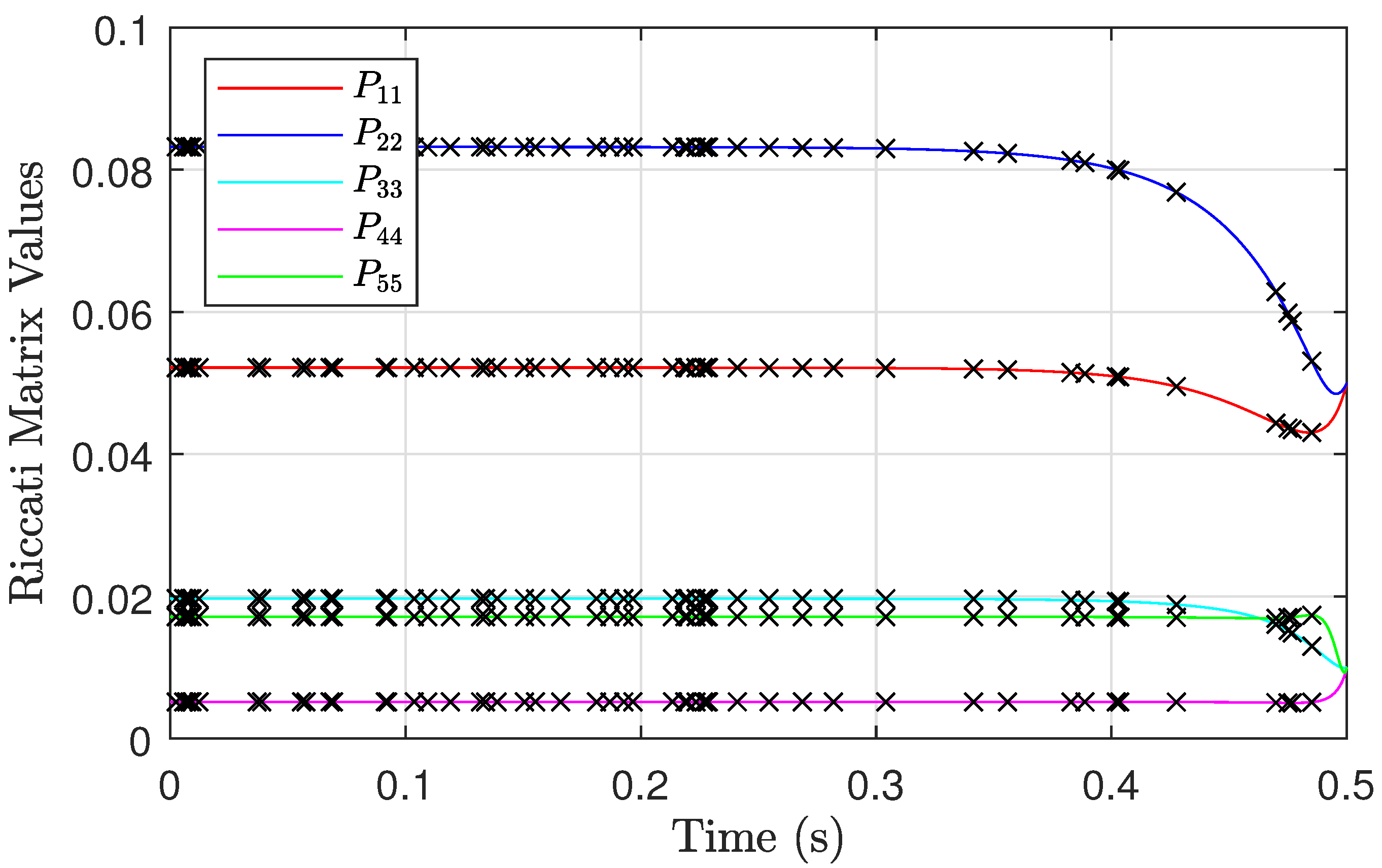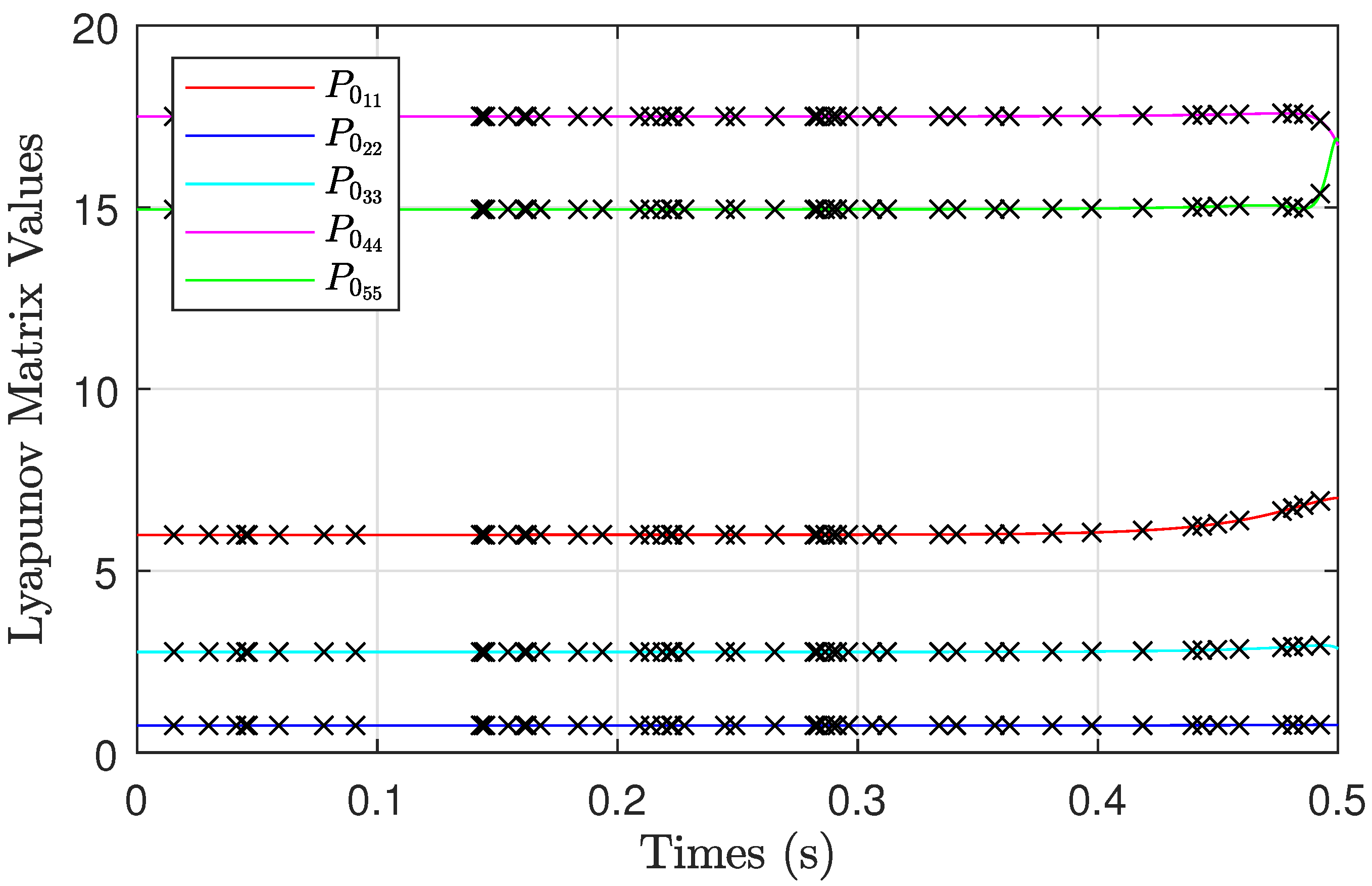Indeed, a global constrained expression with large N and L values resulted in singular $\left(\mathbb{J}{\left({\Xi }_k\right)}^{⊺}\mathbb{J}\left({\Xi }_k\right)\right)$ and $\left({\mathit{H}}^{⊺}\mathit{H}\right)$ matrices within Equations (32) and (35). A subinterval period of $h=0.001$ s, $N=20$, and $L=15$ provided near-perfect results. 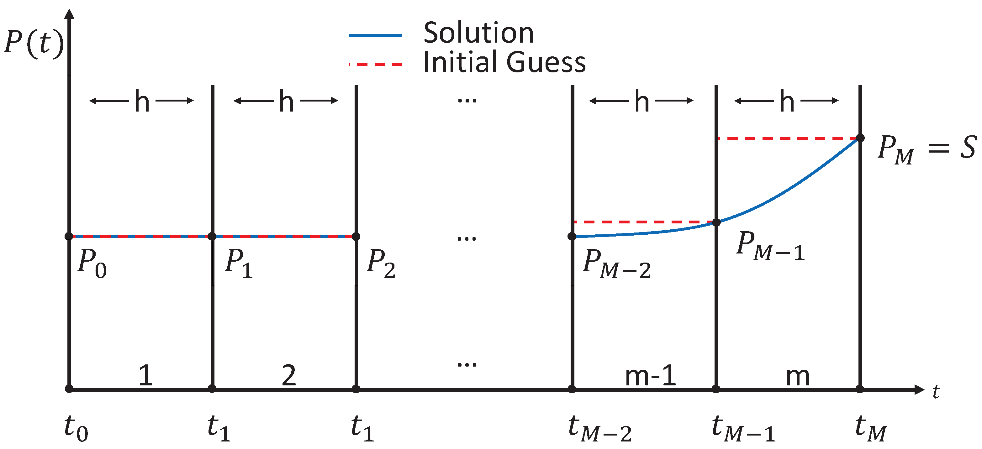The MDRE and MDLE trajectories when such a value of h was used are presented in Figure 2 and Figure 3. The predicted values of the PINN, once it was trained, are also shown in those two figures. As one can see, the predicted values at various time instances (i.e., test points never seen before by the PINN during training) for both the Riccati and Lyapunov diagonal elements match up with the trained solution. This is important because the main benefit of using X-TFC to solve the MDRE or MDLE is that the combined constrained expressions represent a closed-form analytical expression of the solution once trained and Theorem 1 is confirmed. Many other methods that numerically solve the MDRE or MDLE require interpolation between the discretization points (e.g., KE, RK4, and NG). One other thing worth mentioning is that a straight line initial guess similar to what is shown in Figure 1 was used to generate Figure 2 and Figure 3.

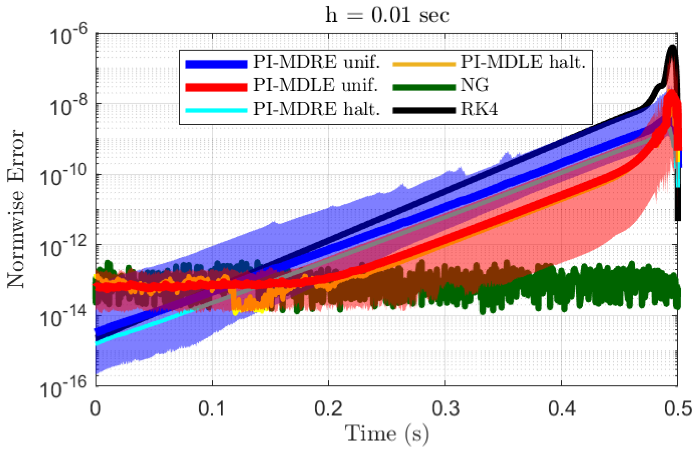
Since our numerical example is taken from Reference [15], we decided to use an identical benchmark as well: the Kalman–Englar (KE) method. More specifically, we computed the L1-normwise errors $\parallel {\mathit{P}}_{\mathrm{exact}}\left(t\right)-\mathit{P}\left(t\right)\parallel /{\mathit{P}}_{\mathrm{exact}}\left(t\right)$. For comparison, these errors were computed from six methods: X-TFC to solve the MDRE with the weight and biases uniformly distributed (PI-MDRE unif.), X-TFC to solve the MDLE with the weight and biases uniformly distributed (PI-MDLE unif.), X-TFC to solve the MDRE with the weight and biases picked from the Halton sequence (PI-MDRE halt.), X-TFC to solve the MDLE with the weight and biases picked from the Halton sequence (PI-MDLE halt.), the Lyapunov approach from Nguyen and Gajic (NG), and the Runge–Kutta 4 method (RK4). When the input weights and biases are uniformly distributed, they are effectively randomized, and the algorithm’s performance will vary between runs. Hence, we performed a Monte Carlo simulation where the uniform distribution varied the input weights and biases. Since the Halton sequence is deterministic, a Monte Carlo simulation was not necessary to quantify its performance. 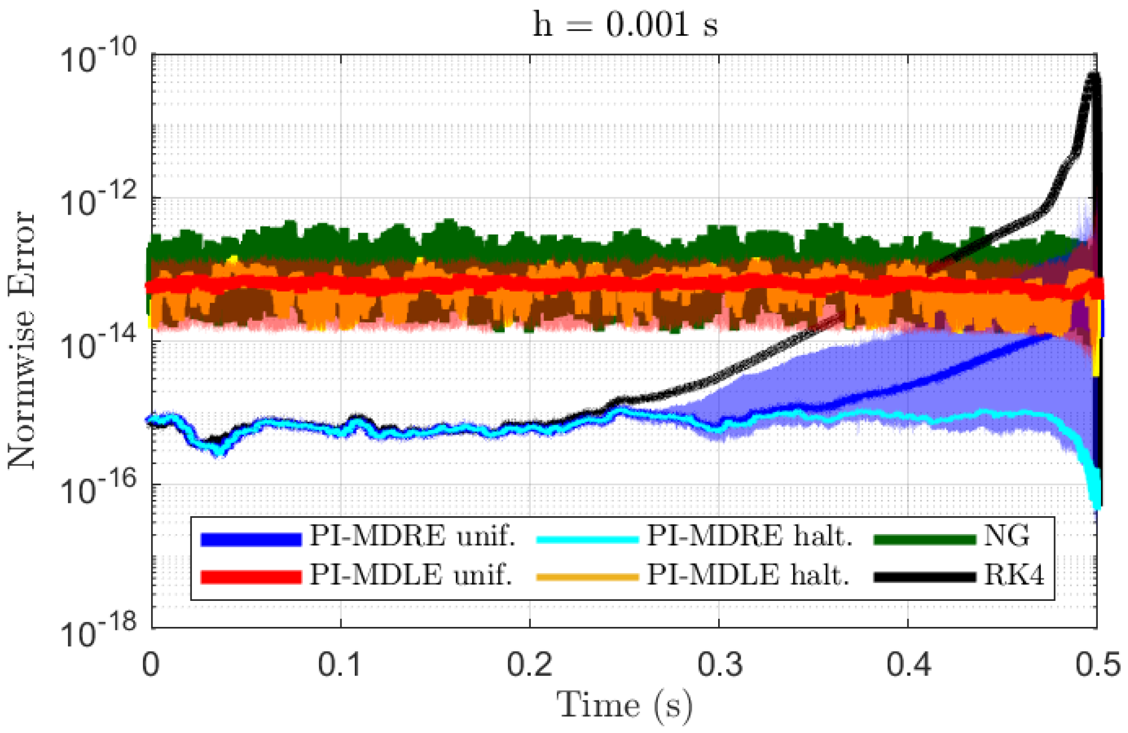Figure 4 and Figure 5 show the L1-normwise errors of the methods when the subinterval time span was selected as $h=0.01$ and $h=0.001$ s, respectively.

We can see from Figure 4 that the NG method is more consistently close to the KE method when $h=0.01$ s. The RK4 and PI-MDRE errors are larger near $t_f$ but decrease below the NG errors once the MDRE solution approaches a straight line near $t_0$. The PI-MDLE errors follow the same trend, except that they mirror the NG error once they are at the same magnitude. Since the PI-MDLE methods approximate the MDLE used in the NG method, this is no surprise. The PI-MDLE errors remain better than RK4’s throughout the entire time domain, while the PI-MDRE unif. errors can be higher than RK4’s. However, if the weight and biases are selected with the Halton sequence, X-TFC is more accurate than RK4 when $h=0.01$ s.

If $h=0.001$, then X-TFC starts to really shine in terms of accuracy. The PI-MDRE unif.’s maximum and PI-MDRE halt. errors were both better than the RK4 and NG errors. The PI-MDLE unif. and PI-MDLE halt. errors were only a slight improvement over NG’s. They did not vary as much between time increments, and their magnitude was slightly lower than the NG method. As can be seen from Figure 2 and Figure 3, the sharpest Riccati and Lyapunov matrix solutions are near $t_f$. This explains why the errors for most of the methods when $h=0.01$ and RK4 when $h=0.001$ were at their worst. Interestingly, the sharp gradients were well approximated by X-TFC for solving the MDRE directly with $h=0.001$. If one wishes to approximate the gradients of the MDRE the most consistently, then using the Halton sequence to sample the input weights and biases would be recommended.

The PI-MDLE errors may not have been as low as those for PI-MDRE, but using X-TFC to compute the MDLE and transforming the Lyapunov solution into the Riccati solution via Equation (16) was faster than solving the MDRE with X-TFC directly. This was because the MDLE is linear, while the MDRE is nonlinear. Thus, X-TFC for computing the MDRE on each subinterval requires multiple iterations of classic linear least squares, while computing the MDLE only needs one. This benefit overcame the extra time-consuming computation needed to obtain the MDRE solution from the MDLE solution. Even if we provide an excellent initial guess to the nonlinear X-TFC solver, the computation still will not achieve the quickness of a linear X-TFC solver. This can be seen in

Table 1. Iteration statistics for PI-MDRE halt. with $h=0.001$ when the initial guess varied.

Initial Guess	Straight Line	RK4
mean (iter.)	9.1800	2.2280
std (iter.)	1.4169	0.7518
min (iter.)	7	2
max (iter.)	24	6

, which shows statistics on the number of iterations it took for PI-MDRE halt. to converge for each subinterval when a straight line and RK4’s solution were used as an initial guess. Note that the input weights and biases were sampled from the Halton sequence for obtaining these measurements, and an $h=0.001$ s was used. All statistics were higher/worse when a nonideal initial guess was used.

The amount of time it took for the various methods to come up with a solution at the training points (i.e., discretization points) and find a solution at the test points (i.e., prediction) is shown in

Table 2. Run time comparison when $h=0.001$.

Method	KE	NG	RK4	PI-MDRE halt.	PI-MDLE halt.
Training (s)	0.4159	1.0894	0.7744	17.5804	1.9576
Prediction (s)	$8.0094\times {10}^{-4}$	$7.8794\times {10}^{-4}$	$7.9004\times {10}^{-4}$	$5.9437\times {10}^{-5}$	$7.6538\times {10}^{-5}$

. The PI-MDRE halt. measurement involved using RK4 as an initial guess. MATLAB’s timeit routine was used to record all run times. Furthermore, MATLAB’s interpn routine, which performs linear interpolation on a vector, was used to compute the KE, NG, and RK4 predictions. We developed our own MATLAB functions to perform PI-MDRE halt. and PI-MDLE halt. prediction. They just consisted of plugging the computed unknowns back into the constrained expressions at the necessary time point. It must also be mentioned that we developed the code for carrying out the training of all methods, and certain coding inconsistencies might warrant the Table 2 comparison to not be utterly fair between the KE, NG, and RK4 methods. Nonetheless, it is very apparent that the PI-MDRE halt. and PI-MDLE halt. runs are not as fast as the state-of-the-art methods. The inversion performed by the least squares step in X-TFC is costly for this numerical example. Still, once the SLFNN is trained, X-TFC can predict the MDRE solution faster than MATLAB’s built-in interpn routine.

As one can see, the PI-MDRE halt. training time was exceptionally high compared to the other methods. Even though the iterative least squares performed for each subinterval were computationally expensive, it was not the main driving force behind PI-MDRE halt.’s high run time. The calculation of the Jacobians via AD with ADiGator ended up being the most computationally expensive, as is shown in

Table 3. Training run time profile for PI-MDRE halt. when $h=0.001$.

Accumulated least squares run time (s)	2.6389
Accumulated AD run time (s)	13.5947
Other run times (s)	1.3504
Total run time (s)	17.5804

. Note that “accumulated” in the table implies all time measurements for each subinterval were summed together. A quicker run time for finding the MDRE solution with X-TFC directly could be achieved by deriving expressions for the Jacobians analytically. We used AD for prototype reasons.

4.1. Varying Subinterval Length

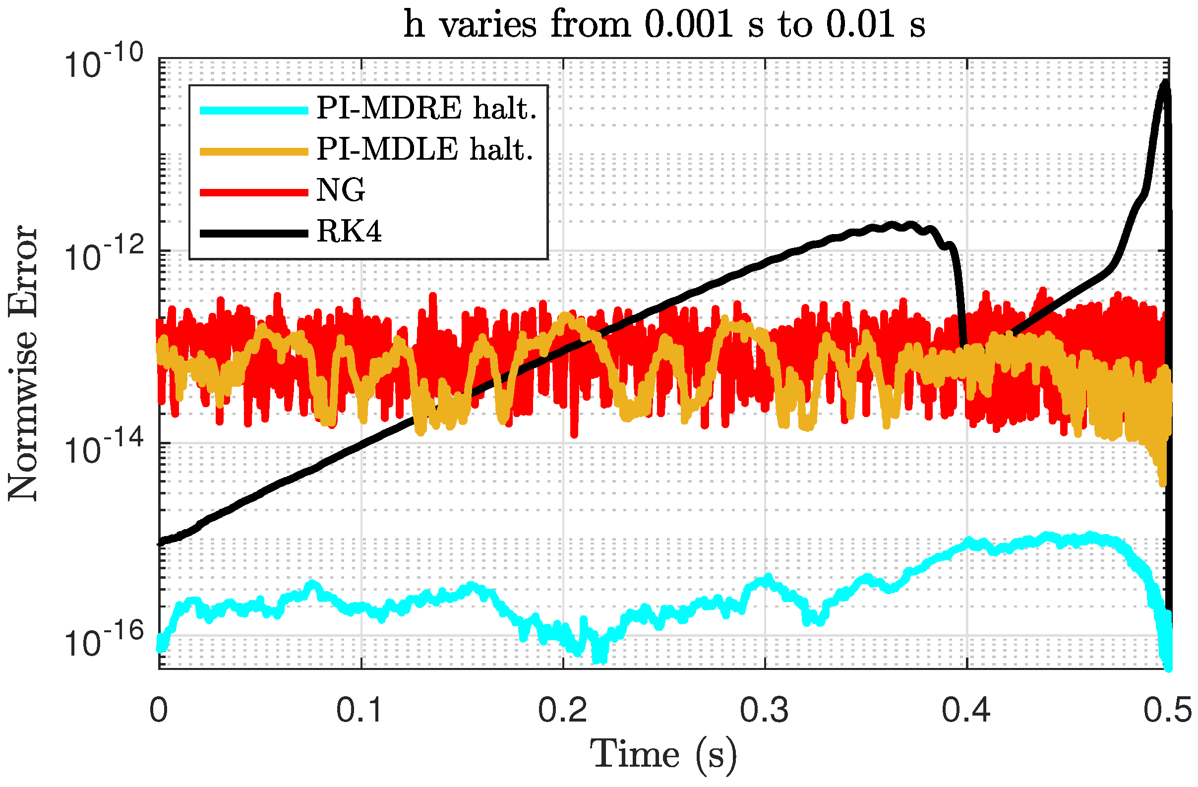
A key question remains: can the execution time of X-TFC be improved while maintaining its accuracy if the subinterval lengths vary? In short, the answer is yes. We decided to keep the subinterval lengths at h = 0.01 s between $t\in [0,0.4]$ and h = 0.001 s between $t\in [0.4,0.5]$, where the solution gradients are the sharpest. As Figure 6 shows, both the PI-MDRE halt. and PI-MDLE halt. errors are similar to when h = 0.001 s for the entire domain (i.e., see Figure 5).

Table 4. Run time comparison when $h=0.001$ from $t\in [0.4,0.5]$ and $h=0.01$ from $t\in [0,0.4]$.

Method	KE	NG	RK4	PI-MDRE halt.	PI-MDLE halt.
Training (s)	0.1147	0.3095	0.2142	7.6390	0.3048
Prediction (s)	$3.1583\times {10}^{-4}$	$2.6559\times {10}^{-4}$	$2.7389\times {10}^{-4}$	$5.5233\times {10}^{-5}$	$7.5128\times {10}^{-5}$

shows that the prediction time with a varying subinterval length remains practically unchanged, but the training times are reduced by more than half when compared with Table 2. The computation time from using X-TFC to solve the MDLE is even competitive with the state-of-the-art numerical methods. Using X-TFC to solve the MDRE is still not competitive in terms of computation time because of the iterative nature of the algorithm. However,

Table 5. Training run time profile for PI-MDRE halt. when $h=0.001$ from $t\in [0.4,0.5]$ and $h=0.01$ from $t\in [0,0.4]$.

Accumulated least squares run time (s)	1.1986
Accumulated AD run time (s)	5.9965
Other run times (s)	0.4439
Total run time (s)	7.6390

shows that its accumulated least squares run time is only about a second. More efficient coding practicing and analytic computation of the Jacobians could drastically reduce PI-MDRE’s total run time to the order of a single second, or even lower, making it as quick as the other state-of-the-art methods.

4.2. Advantages and Disadvantages of X-TFC Compared with State-of-the-Art Methods

The previous numerical study compared solving the MDRE with X-TFC directly and indirectly with the KE, NG, and RK4 methods. How well they compared with X-TFC in terms of accuracy (using the KE method as a benchmark) and computation time was discussed in detail. Here they are summarized for clarity.

The main advantage of using X-TFC to solve the MDRE directly is that its error is consistently near machine-level throughout the domain when the subinterval length is suitably small, along subintervals that contain sharp gradients, and when the Halton sequence is used to initialize the input weights and biases. If the input weights and biases are randomized, then the solution obtained may be worse than the NG method along subintervals that contain sharp gradients. However, our results show it is still better than the RK4 method. Thus, PI-MDRE halt. is the most accurate between the NG and RK4 methods, as long as the the subinterval length is small. When the subinterval length is large, the NG method is the most accurate. The main disadvantage of using X-TFC to solve the MDRE directly is that its computation run time during training is one to two orders of magnitude higher than the state-of-the-art methods. This is due to the iterative nature of the algorithm and the Jacobian computations with AD. Future work should involve computing the Jacobians analytically.

Solving the MDRE indirectly with X-TFC by solving the MDLE significantly speeds up training time. Its training time is even more competitive with the state-of-the-art methods than when solving the MDRE directly. Regardless, solving the MDRE indirectly with X-TFC is only slightly more accurate than the NG method when a small subinterval length is used (i.e., less standard deviation throughout the domain, see Figure 5). Thus, if one is using X-TFC to solve the MDRE, one should do so directly if accuracy is the primary concern and indirectly if computational speed is needed. Still, though, the training speed achieved appears to not be better than the state-of-the-art methods. Although X-TFC, whether solving the MDRE directly or indirectly, is not as fast during training as the state-of-the-art methods, it is faster when predicting the solution on points not seen during training. This is possible because X-TFC gives a closed-form solution. The solution provided by the state-of-the-art methods is not closed-form and requires interpolation to generalize.

One way that was explored in which the speed of X-TFC for solving the MDRE can be improved while still maintaining machine-level accuracy is by varying the subinterval lengths. Large subintervals during regions of the domain where the solution is the most smooth allows for fewer computations to be performed, which speeds up run time. Since the solution on those subintervals is very smooth, it is still well approximated with small SLFNN. For regions of the domain where the solution is not very smooth, containing relatively sharp gradients, a small subinterval is still needed to achieve machine-level accuracy throughout the domain of the solution. Indeed, future work will involve adaptively determining the subinterval length such that it can be as large as possible while keeping the accuracy as low as possible.

5. Conclusions

How X-TFC, a PINN with functional interpolation, can be used to solve the MDRE directly and indirectly by solving an MDLE has been shown. In addition, comparisons between each proposed approach and several other methods (e.g., KE, NG, and RK4) have been made. The purpose of the comparison was to determine the accuracy and computational efficiency of both proposed approaches. Employing X-TFC to solve the MDRE directly yielded the best accuracy amongst all other approaches when the time domain was decomposed into short intervals and the hyperparameters of the network were initialized with a deterministic sequence. When X-TFC was used to solve the MDRE indirectly by solving the MDLE, the accuracy of the former proposed approach could not be matched but was still slightly better than the NG method. It is also worth mentioning that the testing error of the proposed approaches was low, validating the maximum bound estimate on X-TFC’s generalization error.

Using X-TFC to solve the MDLE was much quicker than solving the MDRE directly. Both proposed approaches were not as quick as the state-of-the-art methods during training with a fixed subinterval length. However, when the subinterval length was varied, such that it was shorter during steeper solution gradients and larger otherwise, using X-TFC to solve the MDLE was nearly as quick as the other approaches. X-TFC for solving the MDRE directly still could not match the speed of the state-of-the-art methods, but computing the Jacobians analytically could reduce its run time more. Even though both proposed approaches did not achieve quicker training times, both achieved quicker run times while predicting the solution than the state-of-the-art methods. Therefore, if a control engineer wishes to design a Riccati controller offline at several points and then predict the control between those points online, X-TFC can be a suitable option. However, solving the MDRE in real time with X-TFC to formulate a closed-loop controller may not be quick enough for many optimal control problems. Future work will attempt to see if adaptively varying the subinterval length fixes this issue. Another option would be to solve the linear TPBVP, shown as Equation (4), with X-TFC. Solving the linear TPBVP will likely be quicker because fewer DEs are present in the TPBVP than are in the MDRE. Furthermore, the domain may not need to be decomposed and solved sequentially. Naturally, X-TFC’s ability to solve this TPBVP will be investigated in future research.

References

1. Kalman, R.E. Contributions to the Theory of Optimal Control. Bol. Soc. Mat. Mex. 1960, 5, 102–119. [Google Scholar]
2. Schiassi, E.; Furfaro, R.; Leake, C.; De Florio, M.; Johnston, H.; Mortari, D. Extreme Theory of Functional Connections: A Fast Physics-Informed Neural Network Method for Solving Ordinary and Partial Differential Equations. Neurocomputing 2021, 457, 334–356. [Google Scholar] [CrossRef]
3. Smith, H.A.; Chase, J.G.; Wu, W.H. Efficient Integration of the Time Varying Closed-Loop Optimal Control Problem. J. Intell. Mater. Syst. Struct. 1995, 6, 529–536. [Google Scholar] [CrossRef]
4. Kenney, C.S.; Leipnik, R.B. Numerical Integration of the Differential Matrix Riccati Equation. IEEE Trans. Autom. Control 1985, 30, 962–970. [Google Scholar] [CrossRef]
5. Choi, C. A Survey of Numerical Methods for Solving Matrix Riccati Differential Equations. In Proceedings of the IEEE Proceedings on Southeastcon, New Orleans, LA, USA, 1–4 April 1990; Volume 2, pp. 696–700. [Google Scholar] [CrossRef]
6. Kwakernaak, H.; Sivan, R. Linear Optimal Control Systems; Wiley-Interscience: New York, NY, USA, 1972; Volume 1, pp. 248–253. [Google Scholar]
7. Davison, E.; Maki, M. The Numerical Solution of the Matrix Riccati Differential Equation. IEEE Trans. Autom. Control 1973, 18, 71–73. [Google Scholar] [CrossRef]
8. Vaughan, D. A Negative Exponential Solution for the Matrix Riccati Equation. IEEE Trans. Autom. Control 1969, 14, 72–75. [Google Scholar] [CrossRef]
9. Laub, A.J. Schur Techniques for Riccati Differential Equations. In Feedback Control of Linear and Nonlinear Systems; Springer: Berlin/Heidelberg, Germany, 1982; pp. 165–174. [Google Scholar] [CrossRef]
10. Lainiotis, D. Generalized Chandrasekhar Algorithms: Time-varying Mmodels. IEEE Trans. Autom. Control 1976, 21, 728–732. [Google Scholar] [CrossRef]
11. Anderson, B.D.O.; Moore, J.B. Linear Optimal Control; Prentice-Hall: Engle-Wood Cliffs, NJ, USA, 1971; Chapter 15. [Google Scholar]
12. Potter, J.E. Matrix Quadratic Solutions. SIAM J. Appl. Math. 1966, 14, 496–501. [Google Scholar] [CrossRef]
13. Potter, J.E.; Vander Velde, W.E. Optimum Mixing of Gyroscope and Star Tracker Data. J. Spacecr. Rocket. 1968, 5, 536–540. [Google Scholar] [CrossRef]
14. Radisavljevic, V. Improved Potter–Anderson–Moore Algorithm for the Differential Riccati Equation. Appl. Math. Comput. 2011, 218, 4641–4646. [Google Scholar] [CrossRef]
15. Nguyen, T.; Gajic, Z. Solving the Matrix Differential Riccati Equation: A Lyapunov Equation Approach. IEEE Trans. Autom. Control 2009, 55, 191–194. [Google Scholar] [CrossRef]
16. Balasubramaniam, P.; Samatht, J.A.; Kumaresan, N.; Kumar, A.V.A. Neuro Approach for Solving Matrix Riccati Differential Equation. Neural Parallel Sci. Comput. 2007, 15, 125–135. [Google Scholar]
17. Balasubramaniam, P.; Abdul Samath, J.; Kumaresan, N.; Vincent Antony Kumar, A. Solution of Matrix Riccati Differential Equation for the Linear Quadratic Singular System Using Neural Networks. Appl. Math. Comput. 2006, 182, 1832–1839. [Google Scholar] [CrossRef]
18. Balasubramaniam, P.; Kumaresan, N. Solution of Generalized Matrix Riccati Differential Equation for Indefinite Stochastic Linear Quadratic Singular System Using Neural Networks. Appl. Math. Comput. 2008, 204, 671–679. [Google Scholar] [CrossRef]
19. Kumaresan, N.; Balasubramaniam, P. Optimal Control for Stochastic Linear Quadratic Singular System Using Neural Networks. J. Process. Control 2009, 19, 482–488. [Google Scholar] [CrossRef]
20. Samath, J.A.; Selvaraju, N. Solution of Matrix Riccati Differential Equation for Nonlinear Singular System Using Neural Networks. Int. J. Comput. Appl. 2010, 1, 48–55. [Google Scholar] [CrossRef]
21. Kumaresan, N. Solution of Generalized Matrix Riccati Differential Equation for Indefinite Stochastic Linear Quadratic Singular Fuzzy System with Cross-Term Using Neural Networks. Neural Comput. Appl. 2012, 21, 497–503. [Google Scholar] [CrossRef]
22. Kollmannsberger, S.; D’Angella, D.; Jokeit, M.; Herrmann, L. Physics-Informed Neural Networks. In Deep Learning in Computational Mechanics; Springer: Berlin/Heidelberg, Germany, 2021; pp. 55–84. [Google Scholar]
23. Cuomo, S.; Di Cola, V.S.; Giampaolo, F.; Rozza, G.; Raissi, M.; Piccialli, F. Scientific Machine Learning through Physics-Informed Neural Networks: Where we are and What’s next. arXiv 2022, arXiv:2201.05624. [Google Scholar] [CrossRef]
24. Mortari, D. The Theory of Connections: Connecting Points. Mathematics 2017, 5, 57. [Google Scholar] [CrossRef]
25. Mortari, D. Least-Squares Solution of Linear Differential Equations. Mathematics 2017, 5, 48. [Google Scholar] [CrossRef]
26. Mortari, D.; Johnston, H.; Smith, L. High Accuracy Least-Squares Solutions of Nonlinear Differential Equations. J. Comput. Appl. Math. 2019, 352, 293–307. [Google Scholar] [CrossRef] [PubMed]
27. Huang, G.B.; Zhu, Q.Y.; Siew, C.K. Extreme Learning Machine: Theory and Applications. Neurocomputing 2006, 70, 489–501. [Google Scholar] [CrossRef]
28. Schiassi, E.; D’Ambrosio, A.; Drozd, K.; Curti, F.; Furfaro, R. Physics-Informed Neural Networks for Optimal Planar Orbit Transfers. J. Spacecr. Rocket. 2022, 59, 834–849. [Google Scholar] [CrossRef]
29. Schiassi, E.; D’Ambrosio, A.; Furfaro, R. Bellman Neural Networks for the Class of Optimal Control Problems With Integral Quadratic Cost. IEEE Trans. Artif. Intell. 2022, 1–10. [Google Scholar] [CrossRef]
30. Pontryagin, L.S. Mathematical Theory of Optimal Processes; Routledge: Oxfordshire, UK, 2018. [Google Scholar]
31. Serbin, S.; Serbin, C. A Time-Stepping Procedure for X ˙ = A1X + XA2 + D, X(0) = C. IEEE Trans. Autom. Control. 1980, 25, 1138–1141. [Google Scholar] [CrossRef]
32. Gajic, Z.; Qureshi, M.T.J. Lyapunov Matrix Equation in System Stability and Control; Dover Publications: New York, NY, USA, 2008. [Google Scholar]
33. De Florio, M.; Schiassi, E.; Ganapol, B.D.; Furfaro, R. Physics-Informed Neural Networks for Rarefied-Gas Dynamics: Thermal Creep Flow in the Bhatnagar–Gross–Krook approximation. Phys. Fluids 2021, 33, 047110. [Google Scholar] [CrossRef]
34. Leake, C.; Johnston, H.; Daniele, M. The Theory of Functional Connections: A Functional Interpolation Framework with Applications; Lulu: Research Triangle, NC, USA, 2022. [Google Scholar]
35. Butcher, J.C. Numerical Methods for Ordinary Differential Equations, 3rd ed.; Fundamentals of Astrodynamics and Applications; John Wiley & Sons: Hoboken, NJ, USA, 2016; Chapter 2; pp. 55–142. [Google Scholar]
36. De Florio, M.; Schiassi, E.; Furfaro, R. Physics-Informed Neural Networks and Functional Interpolation for Stiff Chemical Kinetics. Chaos Interdiscip. J. Nonlinear Sci. 2022, 32, 063107. [Google Scholar] [CrossRef] [PubMed]
37. Mishra, S.; Molinaro, R. Estimates on the Generalization Error of Physics-Informed Neural Networks for Approximating PDEs. arXiv 2022, arXiv:2006.16144. [Google Scholar] [CrossRef]
38. Stoer, J.; Bulirsch, R. Introduction to Numerical Analysis, 3rd ed.; Springer: Berlin/Heidelberg, Germany, 2002; Chapter 3. [Google Scholar]
39. Arkun, Y.; Ramakrishnan, S. Bounds on the Optimum Quadratic Cost of Structure-Constrained Controllers. IEEE Trans. Autom. Control 1983, 28, 924–927. [Google Scholar] [CrossRef]
40. Weinstein, M.J.; Rao, A.V. Algorithm 984: ADiGator, a Toolbox for the Algorithmic Differentiation of Mathematical Functions in MATLAB Using Source Transformation via Operator Overloading. Acm Trans. Math. Softw. (TOMS) 2017, 44, 1–25. [Google Scholar] [CrossRef]
Figure 1. FVP domain decomposition diagram.
Mathematics 11 03635 g001
Figure 2. The computed Ricatti matrix diagonal elements. Crossmarks indicate predictions at test points.
Mathematics 11 03635 g002
Figure 3. The computed Lyapunov matrix diagonal elements. Crossmarks indicate predictions at test points.
Mathematics 11 03635 g003
Figure 4. The L 1 -normwise errors between various numerical methods and the KE benchmark for solving the MDRE when the time horizon equaled 0.01 s. The PI-MDRE unif. and PI-MDLE unif. lines are the means from 100 Monte Carlo simulations where the input weights and biases were randomized each time. The boundary of the shaded regions represent the minimum and maximum of the errors from those simulations.
Mathematics 11 03635 g004
Figure 5. The L 1 -normwise errors between various numerical methods and the KE benchmark for solving the MDRE when the time horizon equaled 0.001 s. The PI-MDRE unif. and PI-MDLE unif. lines are the means from 100 Monte Carlo simulations where the input weights and biases were randomized each time. The boundary of the shaded regions represent the minimum and maximum of the errors from those simulations.
Mathematics 11 03635 g005
Figure 6. The L 1 -normwise errors between various numerical methods and the Kalman–Englar benchmark for solving the MDRE when h = 0.001 s from t [ 0.4 , 0.5 ] and h = 0.01 s from t [ 0 , 0.4 ] .
Mathematics 11 03635 g006