Partially Functional Linear Models with Linear Process Errors

Abstract

In this paper, we focus on the partial functional linear model with linear process errors deduced by not necessarily independent random variables. Based on Mercer’s theorem and Karhunen–Loève expansion, we give the estimators of the slope parameter and coefficient function in the model, establish the asymptotic normality of the estimator for the parameter and discuss the weak convergence with rates of the proposed estimators. Meanwhile, the penalized estimator of the parameter is defined by the SCAD penalty and its oracle property is investigated. Finite sample behavior of the proposed estimators is also analysed via simulations.

1. Introduction

Over the last two decades, there has been an increasing interest in functional data analysis due to its extensive application in biometrics, chemometrics, econometrics, medical research as well as other fields. The functional data are intrinsically infinite in dimension; thus, the classical methods for multivariate observations are no longer applicable. The functional linear model is an important model in functional data analysis, and has been extensively investigated. Ramasy and Silverman [1] systematically introduced the statistical analysis methods for the functional data and described regression relationship between functional covariates and scalar responses by the functional linear models; further investigations include Cardot et al. [2], Cardot and Sarda [3], Li and Hsing [4], and Hall and Horowitz [5], who constructed estimator of slope function in the functional linear model and established its convergence with rates based on the functional principal component analysis (FPCA) technique. For more analysis on the functional data, refer to Hall and Hosseini-Nasab [6], Horváth and Kokoszka [7], Hsing and Eubank [8], Ferraty and Vieu [9], and others.

In real data, the response variable is also affected by other covariates. Shin [10] proposed the following partial functional linear model:

$$Y={\mathbf{z}}^T\mathit{\beta }+{\int }_0^1\gamma \left(t\right)X\left(t\right)dt+V,$$

(1)

where $Y\in \mathbb{R}$ is the response variable, $\mathbf{z}$ is a d-dimensional covariate vector with $E\mathbf{z}=0$, $X\left(t\right)$ is a square integrable stochastic process on [0, 1] with $EX\left(t\right)=0$, $\mathit{\beta }$ is an unknown d-dimensional parametric vector, $\gamma \left(t\right)$ is a square integrable unknown coefficient function and V is the regression error, which is independent of $\left\{X\right(t),\mathbf{z}\}$.

The spline method, which is frequently employed to investigate functional data, were used in many papers that studied functional data. Based on B-spline, Yuan and Zhang [11] used the residual sum of squares to construct the test statistic of the $\mathit{\beta }$ in the model (1); Hu and Liang [12] considered the empirical likelihood in the single-index partially functional linear model when the observations are missing at random; Jiang and Huang [13]) discussed single-index partially functional linear quantile regression and used B-spline to approximate the link function and the slope function and further establish the convergence rates and asymptotic normality of the estimators. Bouka et al. [14] employed a smoothing spline to study the estimators with a spatial functional linear regression.

However, the spline method has some drawbacks, such as the fact that shifting a control point causes the entire curve to change, making it hard to regulate the curve’s trend locally. Then, in recent years, many researchers have developed an interest in the FPCA approach for analyzing functional data, since this approach enables finite dimensional study of a topic that is inherently infinitely dimensional. The estimation and testing of a partially functional linear varying coefficient model were covered by Feng and Xue [15]. Based on FPCA, Xie et al. [16] examined the rank-based test’s asymptotic characteristics while considering the hypothesis test for the $\mathit{\beta }$ in the model (1). In addition, Hu et al.’s [17] research also concentrated on the estimation issues for additive partial functional linear models with skew-normal errors. Tang et al. [18] proposed a two-step estimation procedure with FPCA in the partial functional partially linear additive model. At the same time, we find there are several papers to discuss penalized estimators related to the partially functional linear model based on FPCA. For instance, Kong et al. [19] applied a group penalty to reduce the effect of significant functional predictors in a high dimension setting; Du et al. [20] analysed estimation and variable selection; Yao et al. [21] selected the important variables based on the SCAD penalty in partially functional linear quantile model; Wu et al. [22] concentrated on building the estimators for the parameter and slope function with the responses being right-censored and the censoring indicators being missing at random, and proposed a variable selection procedure by the method of adaptive lasso penalty.

It is known that the independence assumption for the model errors, in practical applications, is not always appropriate, especially for sequentially collected economic data, which often exhibit dependence in the errors. Up to now, we have found that Wang et al. [23] established asymptotic normality and weak convergence with rates of the estimators for $\mathit{\beta }$ and $\gamma$, respectively, in model (1) when the errors form a stationary $\alpha$-mixing sequence, while Hu and Liang [24] used the reproducing kernel Hilbert space technique to study the parameter estimator and the convergence rate of the estimator for the slope function with missing observations under under correlated errors $V_i={\sum }_{j=-\infty }^{+\infty }{c}_j{e}_{i-j}$, which is called linear process, with ${\sum }_{j=-\infty }^{+\infty }\left|c_j\right|<\infty$, and further defined the penalized estimator of the parameter by the SCAD penalty and a test statistic for check a linear hypothesis.

Motivated by the discussion in Hu and Liang [24], we, in this paper, focus on the partially functional linear model (1) when the regression error V is a linear process deduced by not necessarily independent random variables by using FPCA method. In particular, we give the estimators $\widehat{\mathit{\beta }}$ and $\widehat{\gamma }(·)$ of $\mathit{\beta }$ and $\gamma (·)$, investigate the asymptotic normality of $\widehat{\mathit{\beta }}$ and discuss the weak convergence with rates of $\widehat{\mathit{\beta }}$ and $\widehat{\gamma }(·)$. At the same time, the penalized estimator of $\mathit{\beta }$ is defined based on the SCAD penalty introduced by Fan and Li [25] and its oracle property is established. Finite sample behavior of the proposed estimators is also investigated via simulations.

The rest of the paper is organized as follows. In Section 2, we construct the estimators of the parameter and slope function including the penalized estimator of the parameter. The main results are described in Section 3. A simulation study is presented in Section 4. Conclusions are put into Section 5. All proofs are put in Section 6.

2. Estimators

2.1. Least Squares Estimation

Let $\{Y_i,X_i\left(t\right),{\mathbf{z}}_i,1\le i\le n\}$ come from $(Y,X(t),\mathbf{z})$ based on model (1), i.e.,

$$Y_i={\mathbf{z}}_i^T\mathit{\beta }+{\int }_0^1\gamma \left(t\right)X_i\left(t\right)dt+V_i,$$

(2)

where $\{X_i\left(t\right),{\mathbf{z}}_i,1\le i\le n\}$ are assume to be i.i.d. random variables, the errors $V_i={\displaystyle \sum _{j=-\infty }^{\infty }}{c}_j{e}_{i-j}$ with ${\displaystyle \sum _{j=-\infty }^{\infty }}\left|c_j\right|<\infty$ and $E{e}_i=0$. Set $C_X(s,t)=EX\left(s\right)X\left(t\right)$. The operator $T_{X}f$ corresponding to $C_X(s,t)$ is defined by

$$\left(T_{X}f\right)(·)={\int }_0^1{C}_X(·,t)f\left(t\right)dt.$$

Then $T_{X}f$ is positive definite, i.e., for $f\in L_2\left([0,1]\right)$, $\langle T_{X}f,f\rangle ={\int }_0^1{\int }_0^{1}EX\left(s\right)X\left(t\right)f\left(s\right)f\left(t\right)dsdt$$=E{\left({\int }_0^{1}X\left(s\right)f\left(s\right)ds\right)}^2\ge 0,$ where $\langle f,g\rangle ={\int }_0^{1}f\left(t\right)g\left(t\right)dt$, $f\left(t\right)$, $g\left(t\right)\in L_2[0,1]$. If $C_X(s,t)$ is continuous, then $C_X(·,·)$ has the following representation by Mercer’s theorem (cf. Hsing and Eubank [8], Theorem 4.6.5, page 120)

$$C_X(s,t)=\sum _{i=1}^{\infty }{\lambda }_i{\rho }_i\left(s\right){\rho }_i\left(t\right),s,t\in [0,1],$$

where $\{{\rho }_i\left(s\right),i\ge 1\}$ is an orthonormal basis of $L_2\left([0,1]\right)$, and $({\lambda }_i,{\rho }_i\left(s\right))$ are (eigenvalue, eigenfunction) pairs of $T_X$, which satisfy $T_X{\rho }_i={\lambda }_i{\rho }_i$, $\langle {\rho }_i,{\rho }_j\rangle =0$ with $i\ne j$ and $\langle {\rho }_i,{\rho }_j\rangle =1$ with $i=j$. Without loss generality, we assume ${\lambda }_1>{\lambda }_2>\cdots >0$. The estimators of $({\lambda }_i,{\rho }_i\left(s\right))$ are defined by

$${\widehat{C}}_X(s,t)=\frac{1}{n}\sum _{i=1}^n{X}_i\left(s\right)X_i\left(t\right)=\sum _{j=1}^{\infty }{\widehat{\lambda }}_j{\widehat{\rho }}_j\left(s\right){\widehat{\rho }}_j\left(t\right),s,t\in [0,1],{\widehat{\lambda }}_1\ge {\widehat{\lambda }}_2\ge \cdots \ge 0,$$

where $\{({\widehat{\lambda }}_j,{\widehat{\rho }}_j),i\ge 1\}$ are the (eigenvalue, eigenfunction) pairs of ${\widehat{T}}_X$ corresponding to ${\widehat{C}}_X$ with ${\widehat{T}}_{X}f(·)={\int }_0^1{\widehat{C}}_X(·,t)f\left(t\right)dt.$ Here, the choice method for $\{{\widehat{\rho }}_j,j\ge 1\}$ is to simply let ${\rho }_j$ take an arbitrary sign while choosing ${\widehat{\rho }}_j$ to minimize $\parallel {\widehat{\rho }}_j-{\rho }_j\parallel$ over the two possible signs, that is, ${\widehat{\rho }}_j$ is chosen so that $\langle {\widehat{\rho }}_j,{\rho }_j\rangle$. Clearly, $\{{\widehat{\rho }}_j,j\ge 1\}$ is an orthonormal basis of $L_2\left([0,1]\right)$ and $\{({\widehat{\lambda }}_j,{\widehat{\rho }}_j),j\ge 1\}$ satisfy ${\widehat{T}}_X{\widehat{\rho }}_j\left(t\right)={\widehat{\lambda }}_j{\widehat{\rho }}_j\left(t\right)$.

In addition, using Karhunen–Loève expansion (cf. Hsing and Eubank [8], Theorem 2.4.13, page 34,), $X\left(t\right)$ and $\gamma \left(t\right)$ have the following expressions

$$X\left(t\right)=\sum _{j=1}^{\infty }\langle X,{\rho }_j\rangle {\rho }_j\left(t\right)=\sum _{j=1}^{\infty }{\theta }_j{\rho }_j\left(t\right),\gamma \left(t\right)=\sum _{j=1}^{\infty }\langle \gamma ,{\rho }_j\rangle {\rho }_j\left(t\right)=\sum _{j=1}^{\infty }{\alpha }_j{\rho }_j\left(t\right),$$

where ${\theta }_j:=\langle X,{\rho }_j\rangle$ and ${\alpha }_j:=\langle \gamma ,{\rho }_j\rangle$. Then $E{\theta }_j=0$ and $\mathrm{Var}\left({\theta }_j\right)={\lambda }_j$. Thus, the model (2) can be written as

$$Y_i={\mathit{\beta }}^{\prime }{\mathbf{z}}_i+\sum _{j=1}^{\infty }{\alpha }_j{\theta }_{ij}+V_i,V_i=\sum _{j=-\infty }^{\infty }{c}_j{e}_{i-j}\mathrm{with}{\theta }_{ij}=\langle X_i,{\rho }_j\rangle .$$

(3)

In order to define the estimators of $\mathit{\beta }$ and $\gamma (·)$, we use an approximated form of (3)

$$Y_i\approx {\mathit{\beta }}^{\prime }{\mathbf{z}}_i+\sum _{j=1}^m{\alpha }_j{\theta }_{ij}+V_i,i=1,2,\cdots ,n,m:=m_n\to \infty (n\to \infty ),$$

which can be rewritten into the following matrix form: $\mathbf{Y}=\mathbf{Z}\mathit{\beta }+{\mathbf{U}}_{\mathbf{m}}\mathbf{\alpha }+\mathbf{V},$ where $\mathbf{Y}={(Y_1,\cdots ,Y_n)}^T$, $\mathbf{Z}=({\mathbf{z}}_1,\cdots ,{{\mathbf{z}}_n)}^T$, ${\mathbf{z}}_i={(z_{i1},\cdots ,z_{id})}^T$, ${\mathbf{U}}_{\mathbf{m}}={\left(\langle X_i,\widehat{{\rho }_j}\rangle \right)}_{n\times m}$, $\mathbf{\alpha }={({\alpha }_i,\cdots ,{\alpha }_m)}^T$, $\mathbf{V}={(V_1,\cdots ,V_n)}^T$. The estimators $(\widehat{\mathit{\beta }},\widehat{\mathbf{\alpha }})$ of $(\mathit{\beta },\mathbf{\alpha })$ can be defined by minimizing the following objective function

$$G(\mathit{\beta },\mathbf{\alpha })={(\mathbf{Y}-\mathbf{Z}\mathit{\beta }-{\mathbf{U}}_{\mathbf{m}}\mathbf{\alpha })}^T(\mathbf{Y}-\mathbf{Z}\mathit{\beta }-{\mathbf{U}}_{\mathbf{m}}\mathbf{\alpha }).$$

Let ${\mathbf{H}}_{\mathbf{m}}={\mathbf{U}}_{\mathbf{m}}{\left({\mathbf{U}}_{\mathbf{m}}^{\mathbf{T}}{\mathbf{U}}_{\mathbf{m}}\right)}^{-\mathbf{1}}{\mathbf{U}}_{\mathbf{m}}^{\mathbf{T}}$. When ${\mathbf{Z}}^{\mathbf{T}}(\mathbf{I}-{\mathbf{H}}_{\mathbf{m}})\mathbf{Z}$ is invertible, we have

$$\begin{array}{c}\hfill \widehat{\mathit{\beta }}={\left({\mathbf{Z}}^T(\mathbf{I}-{\mathbf{H}}_{\mathbf{m}})\mathbf{Z}\right)}^{-1}{\mathbf{Z}}^T(\mathbf{I}-{\mathbf{H}}_{\mathbf{m}})\mathbf{Y},\widehat{\mathbf{\alpha }}={\left({\mathbf{U}}_{\mathbf{m}}^{\mathbf{T}}{\mathbf{U}}_{\mathbf{m}}\right)}^{-1}{\mathbf{U}}_{\mathbf{m}}^{\mathbf{T}}(\mathbf{Y}-\mathbf{Z}\widehat{\mathit{\beta }}).\end{array}$$

Let ${\delta }_{jk}$ denote the Kronecker delta, then

$$\begin{array}{c}\hfill \sum _{i=1}^n\langle X_i,{\widehat{\rho }}_j\rangle \langle X_i,{\widehat{\rho }}_k\rangle =n{\int }_0^1{\int }_0^1{\widehat{C}}_X(s,t){\widehat{\rho }}_j\left(s\right){\widehat{\rho }}_k\left(t\right)dsdt=n{\widehat{\lambda }}_j{\delta }_{jk},\end{array}$$

which implies ${{\mathbf{U}}_{\mathbf{m}}}^T{\mathbf{U}}_{\mathbf{m}}=\mathrm{diag}(n{\widehat{\lambda }}_1,n{\widehat{\lambda }}_2,\cdots ,n{\widehat{\lambda }}_m)$. Put ${\widehat{C}}_{\mathbf{z}}=\frac{1}{n}{\sum }_{i=1}^n{\mathbf{z}}_i{\mathbf{z}}_i^T$, ${\widehat{C}}_{\mathbf{z}Y}=\frac{1}{n}{\sum }_{i=1}^n{\mathbf{z}}_i{Y}_i$,

$$\begin{array}{c}\hfill {\widehat{C}}_{\mathbf{z}X}\left(t\right)=\frac{1}{n}\sum _{i=1}^n{\mathbf{z}}_i{X}_i\left(t\right),{\widehat{C}}_{X\mathbf{z}}\left(t\right)={\left({\widehat{C}}_{\mathbf{z}X}\left(t\right)\right)}^T,{\widehat{C}}_{YX}\left(t\right)=\frac{1}{n}\sum _{i=1}^n{Y}_i{X}_i\left(t\right).\end{array}$$

Then $\widehat{\mathit{\beta }}$ and $\widehat{\mathbf{\alpha }}$ can be rewritten, respectively, as

$$\begin{array}{cc}\hfill \widehat{\mathit{\beta }}& ={\left({\widehat{C}}_{\mathbf{z}}-\sum _{j=1}^m\frac{〈{\widehat{C}}_{\mathbf{z}X},{\widehat{\rho }}_j〉〈{\widehat{C}}_{X\mathbf{z}},{\widehat{\rho }}_j〉}{{\widehat{\lambda }}_j}\right)}^{-1}\left({\widehat{C}}_{\mathbf{z}Y}-\sum _{j=1}^m\frac{〈{\widehat{C}}_{\mathbf{z}X},{\widehat{\rho }}_j〉〈{\widehat{C}}_{YX},{\widehat{\rho }}_j〉}{{\widehat{\lambda }}_j}\right),\hfill \\ \hfill \widehat{\mathbf{\alpha }}& ={\left(\frac{〈{\widehat{C}}_{YX}-{\widehat{\mathit{\beta }}}^T{\widehat{C}}_{\mathbf{z}X},{\widehat{\rho }}_j〉}{{\widehat{\lambda }}_j}\right)}_{j=1,2,\cdots ,m}:=({\widehat{\alpha }}_1,{\widehat{\alpha }}_2,\cdots ,{\widehat{\alpha }}_m),\hfill \end{array}$$

(4)

where $〈{\widehat{C}}_{\mathbf{z}X},{\widehat{\rho }}_j〉=\frac{1}{n}{\sum }_{i=1}^n{\mathbf{z}}_i\langle X_i,{\widehat{\rho }}_j\rangle$ and $〈{\widehat{C}}_{YX},{\widehat{\rho }}_j〉=\frac{1}{n}{\sum }_{i=1}^n{Y}_i\langle X_i,{\widehat{\rho }}_j\rangle$. The estimator $\widehat{\gamma }\left(t\right)$ of $\gamma \left(t\right)$ is defined by $\widehat{\gamma }\left(t\right)={\sum }_{j=1}^m{\widehat{\alpha }}_j{\widehat{\rho }}_j\left(t\right).$

2.2. Variable Selection

Variable selection is a crucial step when the dimensionality of the covariate $\mathbf{z}$ in (1) is high, and it is of great interest to identify the nonzero components in $\mathit{\beta }$. In this paper, we adopt the SCAD penalty introduced by Fan and Li [25] to get a penalized estimator. In particular, the first order derivative of the SCAD penalty function $p_{\omega }\left(t\right)$ is

$$\begin{array}{c}\hfill p_{\omega }^{\prime }\left(t\right)=\omega \left\{I(t\le \omega )+\frac{{(a\omega -t)}_{+}}{(a-1)\omega }I(t>\omega )\right\},t>0,\end{array}$$

where $\omega$ is a tuning parameter and $a=3.7$ suggested by Fan and Li [25]. Hence, we define the penalty estimator of $\mathit{\beta }$ as

$$\begin{array}{c}\hfill {\widehat{\mathit{\beta }}}_p=arg\underset{\mathit{\beta }\in {\mathbb{R}}^d}{min}{G}_p\left(\mathit{\beta }\right):=arg\underset{\mathit{\beta }\in {\mathbb{R}}^d}{min}\left\{G(\mathit{\beta },\alpha \left(\mathit{\beta }\right))+n\sum _{j=1}^d{p}_{\omega }\left(\right|{\beta }_j\left|\right)\right\},\end{array}$$

(5)

where $\alpha \left(\mathit{\beta }\right)={\left({\mathbf{U}}_{\mathbf{m}}^{\mathbf{T}}{\mathbf{U}}_{\mathbf{m}}\right)}^{-1}{\mathbf{U}}_{\mathbf{m}}^{\mathbf{T}}(\mathbf{Y}-\mathbf{Z}\mathit{\beta })$ and ${\beta }_j$ is the j-th component of $\mathit{\beta }$.

Remark 1. 

In simulation below, the tuning parameter ω in (5) is selected by 10-fold cross-validation.

Let ${\mathit{\beta }}_0=({\beta }_{01},\cdots ,{\beta }_{0d})$ be true value of $\mathit{\beta }$, and put $\mathcal{A}=\{j:{\beta }_{0j}\ne 0\}$, $d_1=\left|\mathcal{A}\right|$. Without loss of generality, we assume ${\mathit{\beta }}_0={({\mathit{\beta }}_{01}^T,{\mathit{\beta }}_{02}^T)}^T$, where ${\mathit{\beta }}_{01}\in {\mathbb{R}}^{d_1}$ and ${\mathit{\beta }}_{02}\in {\mathbb{R}}^{d-d_1}$ are the nonzero and zero components of ${\mathit{\beta }}_0$, respectively, i.e., ${\mathit{\beta }}_0={({\mathit{\beta }}_{01}^T,{\mathbf{0}}^T)}^T$, and the estimator of ${\mathit{\beta }}_0={({\mathit{\beta }}_{01}^T,{\mathbf{0}}^T)}^T$ is defined by ${\widehat{\mathit{\beta }}}_p={({\widehat{\mathit{\beta }}}_{p1}^T,{\widehat{\mathit{\beta }}}_{p2}^T)}^T$.

3. Main Results

In the sequel, let $C,C_1,\cdots$ and $c_0,c,c_1,\cdots$ denote generic finite positive constants, whose values may change from line to line; $a_n\sim b_n$ means $C_1\le \frac{a_n}{b_n}\le C_2$; $\parallel f\parallel ={\left({\int }_0^1{f}^2\left(t\right)dt\right)}^{1/2}$. For the sake of convenience for statement, we give the following notations.

$$\begin{array}{cc}\hfill & {\eta }_{ik}=z_{ik}-\langle f_k,X_i\rangle =z_{ik}-\sum _{j=1}^{\infty }\frac{\langle C_{z_{k}X},{\rho }_j\rangle \langle {\rho }_j,X_i\rangle }{{\lambda }_j},{\mathit{\eta }}_i={({\eta }_{i1},{\eta }_{i2},\cdots ,{\eta }_{id})}^T,C_{\mathbf{z}}=\mathrm{Var}\left(\mathbf{z}\right),\hfill \\ \hfill & C_{\mathbf{z}X}={(C_{z_{1}X},\cdots ,C_{z_{d}X})}^T,C_{X\mathbf{z}}={\left(C_{\mathbf{z}X}\right)}^T,f_k=\sum _{j=1}^{\infty }\frac{\langle C_{z_{k}X},{\rho }_j\rangle {\rho }_j}{{\lambda }_j},\mathrm{where}{C}_{z_{k}X}=\mathrm{Cov}(z_k,X)\hfill \end{array}$$

and ${\parallel \mathbf{z}\parallel }_{{\mathbb{R}}^d}^2=z_1^2+z_2^2+\cdots +z_d^2$ for $\mathbf{z}={(z_1,z_2,\cdots ,z_d)}^T$.

In order to list the main results in this paper, we impose the following assumptions.

(A0)

Let random variables $\left\{e_i\right\}$ be identical distributed with $E{e}_1^2<\infty$ or square uniformly integrable and satisfy $E{e}_i=0$.

(A1)

${\int }_0^1{X}^2\left(t\right)dt<\infty$ a.s., and ${E\parallel X\parallel }^4<\infty$.

(A2)

${E\parallel \mathbf{z}\parallel }_{{\mathbb{R}}^d}^4<\infty$.

(A3)

For each j, $E{\theta }_j^4\le c{\lambda }_j^2$ and $c_1{j}^{-a}\le {\lambda }_j\le c_2{j}^{-a}$, ${\lambda }_j-{\lambda }_{j+1}\ge c{j}^{-a-1}$ for some $a>1$.

(A4)

For each j and some $b>\frac{a}{2}+1$: (i) $|{\alpha }_j|\le c{j}^{-b}$; (ii) $|\langle C_{z_{k}X},{\rho }_j\rangle |\le c{j}^{-(a+b)}$ for each k.

(A5)

$m\sim n^{\frac{1}{a+2b}}$.

(A6)

Let ${\eta }_{1k},{\eta }_{2k},\cdots ,{\eta }_{nk}$ be i.i.d. random variables and satisfy $E\left({\eta }_{1k}\right|X_1,X_2,\cdots ,X_n)=0$ a.s., $E\left({\eta }_{1k}^2\right|X_1,X_2,\cdots ,X_n)=B_{kk}$ a.s., which is k-th diagonal element of $\mathbf{B}=E\left({\mathit{\eta }}_i{\mathit{\eta }}_i^T\right)$ and $\mathbf{B}$ is a positive definite matrix. Assume that $E|{\eta }_{1k}{|}^{2+\delta }<\infty$ for $\delta >0$.

(A7)

$\underset{n\to \infty }{lim\; inf}\underset{\theta \to 0^{+}}{lim\; inf}{p}_{\omega }^{\prime }\left(\theta \right)/\omega >0$, $\underset{j\in \mathcal{A}}{max}{p}_{\omega }^{\prime }\left(\right|{\beta }_{0j}\left|\right)=o\left(n^{-1/2}\right)$, $\underset{j\in \mathcal{A}}{max}{p}_{\omega }^{″}\left(\right|{\beta }_{0j}\left|\right)=o\left(1\right)$.

Remark 2. 

(a) 

It is easy to verify $\mathbf{B}=C_{\mathbf{z}}-{\sum }_{j=1}^{\infty }\frac{\langle C_{\mathbf{z}X},{\rho }_j\rangle \langle {\rho }_j,X_i\rangle }{{\lambda }_j}$.

(b) 

(A1)–(A3), (A4)(i), (A5) and (A6) are general regularization conditions in the partially functional linear model (cf. Shin [10]); when ${\lambda }_j$ decrease in (A3), ${\lambda }_j-{\lambda }_{j+1}\ge c{j}^{-a-1}$ implies ${\lambda }_j\ge c_1{j}^{-a}$. (A1) implies $⫴{\widehat{C}}_X-C_X{⫴}^2:={\int }_0^1{\int }_0^1{[{\widehat{C}}_X(s,t)-C_X(s,t)]}^{2}dsdt=O_p\left(n^{-1}\right)$. In fact,

$$\begin{array}{cc}\hfill & E⫴{\widehat{C}}_X-C_X{⫴}^2={\int }_0^1{\int }_0^{1}E{\left[n^{-1}\sum _{i=1}^n{X}_i\left(s\right)X_i\left(t\right)-EX\left(s\right)X\left(t\right)\right]}^{2}dsdt\hfill \\ \hfill & =n^{-1}{\int }_0^1{\int }_0^1\mathrm{Var}\left(X\left(s\right)X\left(t\right)\right)dsdt\le n^{-1}E{\left({\int }_0^1{X}^2\left(s\right)ds\right)}^2=n^{-1}E{\parallel X\parallel }^4=O\left(n^{-1}\right),\hfill \end{array}$$

which implies $⫴{\widehat{C}}_X-C_X{⫴}^2=O_p\left(n^{-1}\right)$.

(c) 

From (A3) and (A4)(ii), we have $|\langle f_k,{\rho }_j\rangle |=|\langle {\sum }_{t=1}^{\infty }\frac{\langle C_{z_{k}X},{\rho }_t\rangle {\rho }_t}{{\lambda }_j},{\rho }_j\rangle |=|\frac{\langle C_{z_{k}X},{\rho }_j\rangle }{{\lambda }_j}|\le c{j}^{-b}.$

Theorem 1. 

Let (A0)–(A6) hold with $E\left(e_i\right|\cdots ,e_{i-2},e_{i-1})=0$ a.s. and $E\left(e_i^2\right|\cdots ,e_{i-2},e_{i-1})={\sigma }^2$ a.s. for $-\infty <i<\infty$. Then $\sqrt{n}(\widehat{\mathit{\beta }}-{\mathit{\beta }}_0)\stackrel{\mathcal{D}}{\to }N\left(0,{\sigma }^2{\mathbf{B}}^{-1}{\sum }_{j=-\infty }^{\infty }{c}_j^2\right).$

Theorem 2. 

Let (A0)–(A6) hold, then $\parallel \widehat{\gamma }{-\gamma \parallel }^2=O_p\left(n^{-(2b-1)/(a+2b)}\right).$

Remark 3. 

When $c_0=1$ and $c_j=0$ for $j\ne 0$, $V_i=e_i$ and $\left\{e_i\right\}$ is i.i.d. random variables, Theorems 1 and 2 can reduce to Theorems 3.1 and 3.2 of Shin [10], respectively.

Theorem 3. 

Suppose that (A0)–(A7) hold. If $\omega \to 0$ and $n^{1/2}\omega \to \infty$, then

(1) 

Selection consistency: $P({\widehat{\mathit{\beta }}}_{p2}=\mathbf{0})\to 1$;

(2) 

Asymptotic normality: If $E\left(e_i\right|\cdots ,e_{i-2},e_{i-1})=0$ a.s. and $E\left(e_i^2\right|\cdots ,e_{i-2},e_{i-1})={\sigma }^2$ a.s. for $-\infty <i<\infty$, then $\sqrt{n}({\widehat{\mathit{\beta }}}_{p1}-{\mathit{\beta }}_{01})\stackrel{\mathcal{D}}{\to }N\left(0,{\sigma }^2{\mathbf{B}}_{p1}^{-1}{\sum }_{j=-\infty }^{\infty }{c}_j^2\right),$ where ${\mathbf{B}}_{p1}=E\left({\mathit{\eta }}_{i\left(1\right)}{\mathit{\eta }}_{i\left(1\right)}^T\right)$ and ${\mathit{\eta }}_{i\left(1\right)}$ is related to ${\mathbf{z}}_{i\left(1\right)}$, which is corresponding to ${\mathit{\beta }}_{01}$, is a $d_1$-dimensional subvector of ${\mathbf{z}}_i$ for $i=1,2,\cdots ,n$.

4. Simulation Study

4.1. Least Squares Estimation

In this subsection, we use the Monte Carlo simulation to study the performance for the proposed methods. The data are generated from the following model:

$$\begin{array}{c}\hfill Y_i=z_{i1}{\beta }_1+z_{i2}{\beta }_2+{\int }_0^1\gamma \left(t\right)X_i\left(t\right)dt+V_i,\end{array}$$

(6)

where $z_{i1}\sim N(0,1)$, $z_{i2}\sim N(0,1)$ and $\mathit{\beta }={({\beta }_1,{\beta }_2)}^T={(1,2)}^T$. Taking $X_i\left(t\right)={\sum }_{j=1}^{50}{\theta }_j{\rho }_j\left(t\right)$, ${\theta }_j\sim N(0,{\lambda }_j)$ and ${\rho }_j\left(t\right)=\sqrt{2}sin\left((j-0.5)\pi t\right)$. For ${\int }_0^1\gamma \left(t\right)X_i\left(t\right)dt={\sum }_{j=1}^m{\theta }_{ij}{\alpha }_j$ in (6), let

$${\alpha }_j={\int }_0^1\gamma \left(t\right){\rho }_j\left(t\right)dt\mathrm{with}\gamma \left(t\right)=\sqrt{2}sin\left(\frac{\pi t}{2}\right)+3\sqrt{3}sin\left(\frac{3\pi t}{2}\right)$$

and m be chosen by the CPV method (see Horváth and Kokoszka [7], page 41), i.e.,

$$m=\underset{k}{min}\{k:\mathrm{CPV}\left(k\right)\ge 85\%\}=\underset{k}{min}\left\{k:\sum _{i=1}^k{\widehat{\lambda }}_i/\sum _{i=1}^n{\widehat{\lambda }}_i\ge 85\%\right\}.$$

Let $V_i$ be an $AR\left(1\right)$ process: $V_i=\varphi V_{i-1}+e_i,$ where $e_i\sim N(0,1)$ and $\left|\varphi \right|<1$. Thus, $E{V}_i^2=1/(1-{\varphi }^2)$.

In the simulation, we take $\varphi =0.1,0.9$ and sample sizes $n=50$ and 200. For each sample size, we replicate $N=500$ simulations and take $l=500$ grid points of equal interval in $[0,1]$. The mean square error (MSE) of the estimators $\widehat{\gamma }(·)$ and $\widehat{\beta }$ of $\gamma (·)$ and $\beta$ is defined, respectively, as

$$\begin{array}{c}\hfill \mathrm{MSE}\left(\widehat{\gamma }\right)=\frac{1}{Nl}\sum _{i=1}^N\sum _{k=1}^l{[{\widehat{\gamma }}_i\left(t_k\right)-{\gamma }_i\left(t_k\right)]}^2,\mathrm{MSE}\left(\widehat{\beta }\right)=\frac{1}{N}\sum _{i=1}^N{[\widehat{\beta }\left(i\right)-\beta ]}^2.\end{array}$$

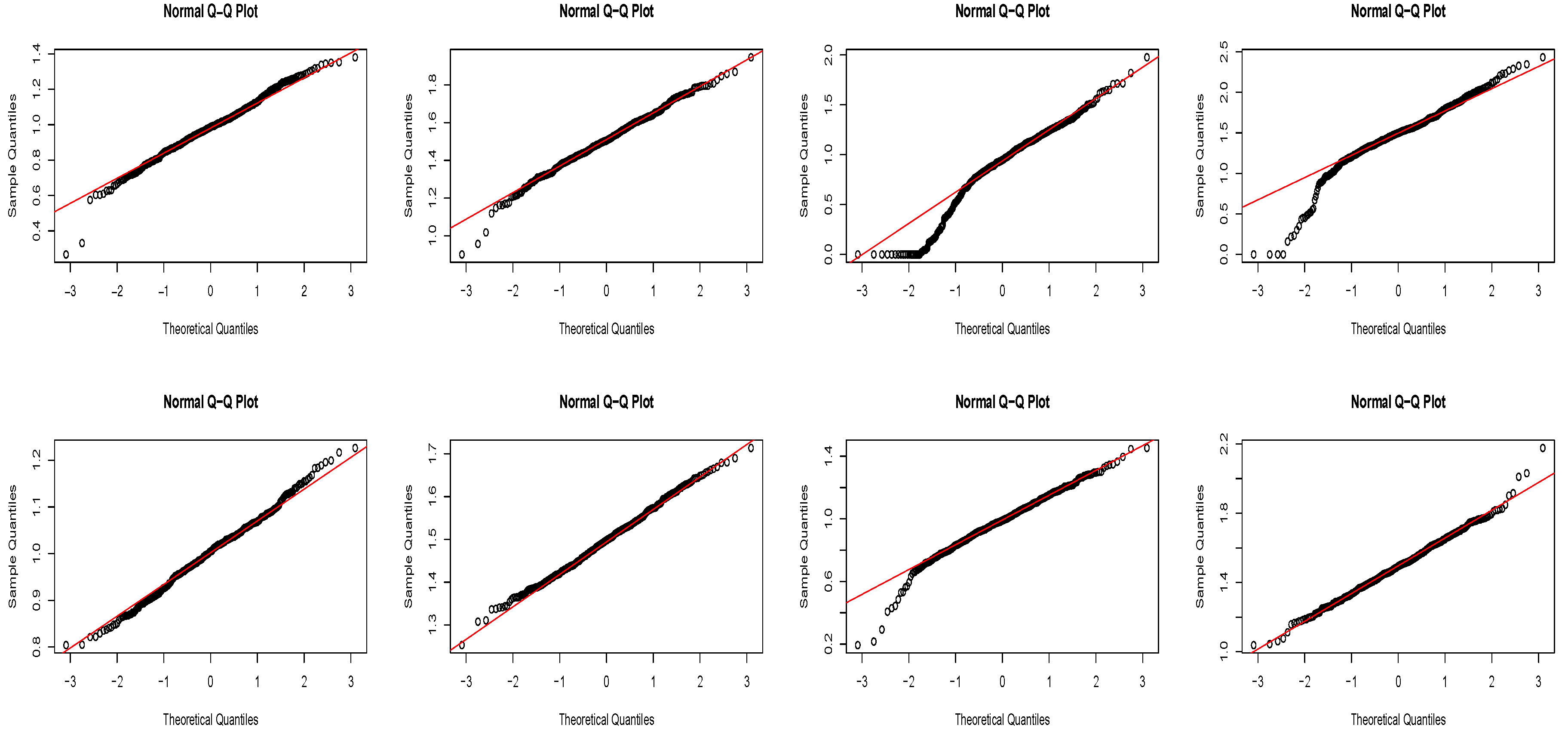
In Figure 1, we draw Q-Q plots of the estimators ${\widehat{\beta }}_1$ and ${\widehat{\beta }}_2$ with sample sizes n = 50, 200 and $\varphi =0.1,0.9$. Figure 1 illustrates that more points fall near the line as $n=200$ and the value of $\varphi =0.1$; more points on either sides are away from the line when $n=50$ and $\varphi =0.9$. This implies the quality of fit decreases as the dependence of the observations increases, i.e., the value of $\varphi$ increases, and that the normality in the distribution of the estimators increases as the sample size n increases, which comfirms the asymptotic normality in Theorem 1.

In

Table 1. Values of bias, MSEs for ${\widehat{\beta }}_1$, ${\widehat{\beta }}_2$ and $\widehat{\gamma }$ with $n=50,200$ and $\varphi =0.1,0.9$.

n	$\mathit{\varphi }$	MSE			Bias
		${\widehat{\mathit{\beta }}}_{\mathbf{1}}$	${\widehat{\mathit{\beta }}}_{\mathbf{2}}$	$\widehat{\gamma }$	${\widehat{\mathit{\beta }}}_{\mathbf{1}}$	${\widehat{\mathit{\beta }}}_{\mathbf{2}}$
50	0.1	0.0207	0.0245	1.8649	0.0040	−0.0050
	0.9	0.1010	0.1288	6.1297	0.0078	−0.0118
200	0.1	0.0051	0.0052	0.4606	0.0044	−0.0058
	0.9	0.0289	0.0268	2.1421	0.0040	−0.0120

, we report the bias and MSEs, of the estimators for ${\beta }_1$, ${\beta }_2$ and $\gamma \left(t\right)$. From Table 1, we can draw the following conclusions:

(1)

For the same sample size n, the values of MSE$\left({\widehat{\beta }}_1\right)$, MSE$\left({\widehat{\beta }}_2\right)$ and $\mathrm{MSE}\left(\widehat{\gamma }\right)$ increase with $\varphi$ increasing;

(2)

With the same $\varphi$, if the sample size n increases, then the values of MSE$\left({\widehat{\beta }}_1\right)$, MSE$\left({\widehat{\beta }}_2\right)$ and $\mathrm{MSE}\left(\widehat{\gamma }\right)$ decrease;

(3)

Changes of the sample size n and $\varphi$ have a little effect on the biases of ${\widehat{\beta }}_1$ and ${\widehat{\beta }}_2$.

4.2. Variable Selection

In this subsection, we add six independent covariates $\{z_{i3},z_{i4},\cdots ,z_{i8}\}$ with $z_{ij}\sim N(0,1)$ ($j=3,4,\cdots ,8$) to model (6), and take $\mathit{\beta }={({\beta }_1,{\beta }_2,\cdots ,{\beta }_8)}^T={(1,2,0,0,0,0,0,0)}^T$. Set C as the average number of components in $\mathit{\beta }$ correctly estimated to be zero, IC as the average number of components in $\mathit{\beta }$ incorrectly estimated to be zero, C-fit as the probability of exactly fitting the model and MSE($\widehat{\mathit{\beta }})=\frac{1}{8N}{\sum }_{j=1}^8{\sum }_{i=1}^N{[{\widehat{\beta }}_j\left(i\right)-{\beta }_j]}^2$ as the mean square error of the estimator for $\mathit{\beta }$.

Figure 2 shows Q-Q plots of the estimators for ${\beta }_1$ and ${\beta }_2$ with $n=50$, 200 and $\varphi =0.1,$ 0.9 by using the SCAD penalty function. The performance from Q-Q plots in this instance is comparable to that in Section 4.1. The asymptotic normality in Theorem 3 is verified as sample size rises because the Q-Q plots are more aligned with the normality; when the value of $\varphi$ is increasing, the poorer imitative impact is observed.

In

Table 2. Values of C, IC, C-fit and MSE($\widehat{\mathit{\beta }})$.

n	$\mathit{\varphi }$	C	IC	C-Fit	MSE($\widehat{\mathit{\beta }})$
50	0.1	4.94	0	0.8675	0.0847
	0.9	4.12	0.048	0.759	0.5204
200	0.1	5.424	0	0.928	0.0173
	0.9	4.982	0	0.873	0.0900

, we represent the values of C, IC, C-fit and MSE($\widehat{\mathit{\beta }})$. Table 2 indicates the following conclusion:

(1)

When the sample size n increases with the same $\varphi$, the value of MSE($\widehat{\mathit{\beta }})$ decreases;

(2)

 

(i)

If the sample size n increases with the same $\varphi$, the average number of zero coefficients correctly estimated to be zero is close to 5 and the average number of components in $\mathit{\beta }$ incorrectly estimated to be zero is near 0 and even is 0 when $\varphi =0.1$ or $n=200$. This verifies the selection consistency in Theorem 3;

(ii)

When the value of $\varphi$ dereases with the same sample size, the average number of zero coefficients correctly estimated to be zero increases, and the average number of components in $\mathit{\beta }$ incorrectly estimated to be zero decreases;

(3)

As the sample size n increases with the same $\varphi$ or $\varphi$ decreases with the same sample size, the probability of exactly fitting the model increases.

5. Conclusions

By using the least square method, based on FPCA, we construct the estimators of parameter and coefficient function in the partially functional linear models with linear process errors and establish asymptotic normality of parameter estimator and the rate of convergence of the estimator for the coefficient function. Additionally, we use the SCAD penalty to define the estimator of the parameter and discuss its oracle property.

However, the proposed method has some limitations. First, in this study, we approximate the expansion of the function part into partial sum form by using the FPCA method, which may leave out data information due to the truncation value m. Second, while, in practice, there exists missing data, this work considers the scenario of complete data. Therefore, in the event of missing data, our proposed method may be inapplicable. In the future, we are interested in figuring out a way to reduce data information loss and take missing data into account.

6. Proof of Main Results

In proof below, we use the following notations: for linear operator T, let ${\parallel T\parallel }_{\infty }=\underset{\parallel f\parallel =1}{sup}\parallel Tf\parallel$, ${\parallel T\parallel }_{\mathcal{H}}=\underset{\parallel f\parallel =1}{sup}\left|Tf\right|$ for $f\in L_2[0,1]$; ${\parallel A\parallel }_{\infty }=\underset{i}{max}{\sum }_j\left|A_{ij}\right|$ for matrix $A=\left(A_{ij}\right)$; for $k=1,\cdots ,d$, set ${\mathit{\eta }}_{\left(k\right)}={({\eta }_{1k},{\eta }_{2k},\cdots ,{\eta }_{nk})}^T$, ${\mathbf{f}}_{\left(k\right)}={(\langle f_k,X_1\rangle ,\langle f_k,X_2\rangle ,\cdots ,\langle f_k,X_n\rangle )}^T$, ${\mathbf{z}}_{\left(k\right)}={(z_{1k},z_{2k},\cdots ,z_{nk})}^T$,

$$\begin{array}{c}\hfill {\widehat{\psi }}_k\left(f\right)=\sum _{j=1}^m\frac{\langle {\widehat{C}}_{z_{k}X},{\widehat{\rho }}_j\rangle \langle {\widehat{\rho }}_j,f\rangle }{{\widehat{\lambda }}_j},{\psi }_k\left(f\right)=\sum _{j=1}^{\infty }\frac{\langle C_{z_{k}X},{\rho }_j\rangle \langle {\rho }_j,f\rangle }{{\lambda }_j},\end{array}$$

$\widehat{\mathbf{B}}=\frac{1}{n}\left({\mathbf{Z}}^T(\mathbf{I}-{\mathbf{H}}_{\mathbf{m}})\mathbf{Z}\right)$ and $\mathbf{M}={\left(\langle \gamma ,X_1\rangle ,\langle \gamma ,X_2\rangle ,\cdots ,\langle \gamma ,X_n\rangle \right)}^T$.

Lemma 1 

(Shin [10] ).

(1) 

Let $E{\theta }_j^4\le c{\lambda }_j^2$, then $E\parallel {\widehat{T}}_X-T_X{\parallel }_{\infty }^2\le n^{-1}E{\parallel X\parallel }^4$, $E\parallel {\widehat{C}}_{\mathbf{z}}-C_{\mathbf{z}}{\parallel }_{\infty }^2\le n^{-1}E{\parallel \mathbf{z}\parallel }_{{\mathbb{R}}^d}^4$ and $E\parallel {\widehat{C}}_{z_{k}X}-C_{z_{k}X}{\parallel }^2\le n^{-1}{\left({E\parallel \mathbf{z}\parallel }_{{\mathbb{R}}^d}^{4}E{\parallel X\parallel }^4\right)}^{1/2}$ for $k=1,2,\cdots ,d.$

(2) 

Suppose that (A1), (A3), (A4)(i), (A5) and (A6) are satisfied. Then $\parallel {\psi }_k-{\widehat{\psi }}_k{\parallel }_{\mathcal{H}}^2=O_p\left(n^{-(2b-1)/(a+2b)}\right).$ Further, if $\left\{e_i\right\}$ are identical distributed with $E{e}_1^2<\infty$ or square uniformly integrable, $\parallel \widehat{\mathbf{B}}{-\mathbf{B}\parallel }_{\infty }^2=O_p\left(n^{-(2b-1)/(a+2b)}\right).$

Lemma 2 

(Pollard [26], page 171). Let $\{Z_{nk},k\ge 0\}$ be a sequence of random variables and $\{{\mathcal{G}}_{n,k-1},k\ge 1\}$ be increasing sequence of σ-fields such that $\left\{Z_{nk}\right\}$ is measurable with respect to ${\mathcal{G}}_{n,k}$, and $E\left(Z_{nk}\right|{\mathcal{G}}_{n,k-1})=0$ for $1\le k\le n$. Assume that ${\sum }_{k=1}^{n}E\left(Z_{nk}^2\right|{\mathcal{G}}_{n,k-1})\stackrel{p}{\to }{a}^2$ and ${\sum }_{k=1}^{n}E\left(Z_{nk}^{2}I\left(|Z_{nk}|>q\right)\right|{\mathcal{G}}_{n,k-1})\stackrel{p}{\to }0$ for some constant $a^2>0$ and every $q>0$. Then ${\sum }_{k=1}^n{Z}_{nk}\stackrel{d}{\to }N(0,a^2)$.

Lemma 3. 

For $t\in [0,1]$, let $\{X_i\left(t\right),i\ge 1\}$ be $i.i.d.$ random variables with $E{X}_i\left(t\right)=0$ and $E\parallel X_1{\parallel }^2<\infty$. Set $V_i={\sum }_{s=-\infty }^{\infty }{c}_s{e}_{i-s}$ with ${\sum }_{j=-\infty }^{\infty }\left|c_j\right|<\infty$. Assume that $\{X_i\left(t\right),i\ge 1\}$ is independent of $\{e_i,i\in \mathbb{Z}\}$, and that $\left\{e_i\right\}$ are identical distributed with $E{e}_1^2<\infty$ or square uniformly integrable. Then $n^{-1/2}\parallel {\sum }_{i=1}^n{X}_i{V}_i\parallel =O_p\left(1\right).$

Proof. 

Note that ${sup}_{i}E{V}_i^2\le {sup}_i\left[{\sum }_{s=-\infty }^{\infty }{c}_s^{2}E{e}_{i-s}^2+2{\sum }_{s=-\infty }^{\infty }{\sum }_{k>s}\left|c_s{c}_k\right|{\left(E{e}_{i-s}^{2}E{e}_{i-k}^2\right)}^{1/2}\right]$ $\le c{\left({\sum }_{s=-\infty }^{\infty }\left|c_s\right|\right)}^2<\infty .$ So $E{\left(n^{-1/2}\parallel {\sum }_{i=1}^n{X}_i{V}_i\parallel \right)}^2=n^{-1}{\sum }_{i=1}^{n}E{\parallel X_i\parallel }^{2}E{V}_i^2<\infty ,$ which yields $n^{-1/2}\parallel {\displaystyle \sum _{i=1}^n}{X}_i{V}_i\parallel =O_p\left(1\right).$ □

Lemma 4. 

If (A1) and $E{\theta }_k^4\le c{\lambda }_k^2$ for each k hold, then $E{P}_k\le c{n}^{-1}{\lambda }_k$ and $E{Q}_{jk}^2\le c{n}^{-1}{\lambda }_j{\lambda }_k$, where $P_K={\int }_0^1{\left({\int }_0^1\left({\widehat{C}}_X(s,t)-C_X(s,t)\right){\rho }_k\left(t\right)dt\right)}^{2}ds$, $Q_{jk}={\int }_0^1{\int }_0^1({\widehat{C}}_X(s,t)-C_X(s,t)){\rho }_j\left(s\right)$${\rho }_k\left(t\right)dsdt$.

Proof. 

From ${\theta }_{ik}=\langle X_i,{\rho }_k\rangle$, using (A1) we have

$$\begin{array}{cc}\hfill E{P}_k=& {\int }_0^{1}E{\left(\frac{1}{n}\sum _{i=1}^n{X}_i\left(s\right){\int }_0^1{X}_i\left(t\right){\rho }_k\left(t\right)dt-EX\left(s\right){\int }_0^{1}X\left(s\right){\rho }_k\left(t\right)dt\right)}^{2}ds\hfill \\ \hfill =& {\int }_0^{1}E{\left(\frac{1}{n}\sum _{i=1}^n{X}_i\left(s\right)\langle X_i,{\rho }_k\rangle -E\left[X\left(s\right)\langle X,{\rho }_k\rangle \right]\right)}^{2}ds\le \frac{1}{n}E\left[{\int }_0^1{X}^2\left(s\right)ds{\theta }_k^2\right]\hfill \\ \hfill =& n^{-1}{E(\parallel X\parallel }^2{\theta }_k^2)\le n^{-1}{\left({E\parallel X\parallel }^4·E{\theta }_k^4\right)}^{1/2}\le c{n}^{-1}{\lambda }_k,\hfill \\ \hfill E{Q}_{jk}^2=& E{\left({\int }_0^1{\int }_0^1\left(\frac{1}{n}\sum _{i=1}^n{X}_i\left(s\right)X_i\left(t\right)-E\left(X\left(s\right)X\left(t\right)\right)\right){\rho }_j\left(s\right){\rho }_k\left(t\right)dsdt\right)}^2\hfill \\ \hfill =& E{\left(\frac{1}{n}\sum _{i=1}^n\langle X_i,{\rho }_j\rangle \langle X_i,{\rho }_k\rangle -E\langle X,{\rho }_j\rangle \langle X\left(t\right),{\rho }_k\rangle \right)}^2=\mathrm{Var}\left(\frac{1}{n}\sum _{i=1}^n{\theta }_{ij}{\theta }_{ik}\right)\hfill \\ \hfill =& n^{-1}\mathrm{Var}\left({\theta }_j{\theta }_k\right)\le n^{-1}{\left(E{\theta }_j^{4}E{\theta }_k^4\right)}^{1/2}\le c{n}^{-1}{\lambda }_j{\lambda }_k.\hfill \end{array}$$

□

Lemma 5. 

Let $\left\{x_n\right\}$ and $\left\{y_n\right\}$ be two sequences of independent random variables, then for any $\epsilon >0$ and $c>0$ we have

$$E|x_n{y}_n{|}^{2}I\left(\right|x_n{y}_n|>\epsilon )\le E|x_n{|}^{2}I\left(\right|x_n|>c)E|y_n{|}^2+E|y_n{|}^{2}I\left(\right|y_n|>\epsilon /c)E|x_n{|}^2.$$

Proof. 

Using independence between $\left\{x_n\right\}$ and $\left\{y_n\right\}$, it follows that

$$\begin{array}{cc}\hfill E|x_n{y}_n{|}^{2}I\left(\right|x_n{y}_n|>\epsilon )& =E|x_n{y}_n{|}^2\left\{I\left(\right|x_n{y}_n|>\epsilon ,|x_n|>c)+I\left(\right|x_n{y}_n|>\epsilon ,|x_n|\le c)\right\}\hfill \\ \hfill & \le E|x_n{|}^{2}I\left(\right|x_n|>c)E|y_n{|}^2+E|y_n{|}^{2}I\left(\right|y_n|>\epsilon /c)E|x_n{|}^2.\hfill \end{array}$$

□

Proof of Theorem 1. 

We write (cf. the proof of Theorem 3.1 in Shin [10])

$$\begin{array}{cc}\hfill \sqrt{n}\left(\widehat{\mathit{\beta }}-{\mathit{\beta }}_0\right)=& n^{-\frac{1}{2}}{\widehat{\mathbf{B}}}^{-1}\{\sum _{i=1}^n\left[{\mathbf{z}}_i-\sum _{j=1}^m\frac{\langle {\widehat{C}}_{\mathbf{z}X},{\widehat{\rho }}_j\rangle \langle {\widehat{\rho }}_j,X_i\rangle }{{\widehat{\lambda }}_j}\right]\langle \gamma ,X_i\rangle \hfill \\ \hfill & +\sum _{i=1}^n\left[\sum _{j=1}^{\infty }\frac{\langle C_{\mathbf{z}X},{\rho }_j\rangle \langle X_i,{\rho }_j\rangle }{{\lambda }_j}-\sum _{j=1}^m\frac{\langle {\widehat{C}}_{\mathbf{z}X},{\widehat{\rho }}_j\rangle \langle {\widehat{\rho }}_j,X_i\rangle }{{\widehat{\lambda }}_j}\right]V_i\hfill \\ \hfill & +\sum _{i=1}^n\left[{\mathbf{z}}_i-\sum _{j=1}^{\infty }\frac{\langle C_{\mathbf{z}X},{\rho }_j\rangle \langle {\rho }_j,X_i\rangle }{{\lambda }_j}\right]V_i\}\hfill \\ \hfill :=& {\widehat{\mathbf{B}}}^{-1}(A_1+A_2+A_3).\hfill \end{array}$$

Lemma 1 implies $\widehat{\mathbf{B}}\stackrel{p}{\to }\mathbf{B}$. Thus, it suffices to show that $A_1=o_p\left(1\right)$, $A_2=o_p\left(1\right)$ and

$$\begin{array}{c}\hfill A_3=n^{-1/2}\sum _{i=1}^n{\mathit{\eta }}_i{V}_i\stackrel{d}{\to }N(0,{\sigma }^2\mathbf{B}\sum _{j=-\infty }^{\infty }{c}_j^2).\end{array}$$

(7)

Step 1. We prove $A_2=o_p\left(1\right)$. By applying Lemmas 1 and 3, it follows

$$\begin{array}{cc}\hfill \parallel A_2{\parallel }_{{\mathbb{R}}^d}=& \parallel n^{-1/2}\sum _{i=1}^n[\sum _{j=1}^{\infty }\frac{\langle C_{\mathbf{z}X},{\rho }_j\rangle \langle X_i,{\rho }_j\rangle }{{\lambda }_j}-\sum _{j=1}^m\frac{〈{\widehat{C}}_{\mathbf{z}X},{\widehat{\rho }}_j〉〈{\widehat{\rho }}_j,X_i〉}{{\widehat{\lambda }}_j}]V_i{\parallel }_{{\mathbb{R}}^d}\hfill \\ \hfill =& n^{-1/2}\parallel {({\psi }_1-{\widehat{\psi }}_1,\cdots ,{\psi }_d-{\widehat{\psi }}_d)}^T\left(\sum _{i=1}^n{X}_i{V}_i\right){\parallel }_{{\mathbb{R}}^d}\hfill \\ \hfill \le & n^{-1/2}\sum _{k=1}^d\parallel {\psi }_k-{\widehat{\psi }}_k{\parallel }_{\mathcal{H}}\parallel \sum _{i=1}^n{X}_i{V}_i\parallel =O_p\left(n^{-\frac{2b-1}{2(a+2b)}}\right)=o_p\left(1\right),\hfill \end{array}$$

which yields $A_2=o_p\left(1\right)$.

Step 2. We prove $A_1=o_p\left(1\right)$. From ${\mathbf{z}}_{\left(k\right)}={\mathit{\eta }}_{\left(k\right)}+{\mathbf{f}}_{\left(k\right)}$, we know that the k-th ($1\le k\le d$) element of $A_1$ is

$$\begin{array}{cc}\hfill A_1\left(k\right)=& n^{-1/2}\sum _{i=1}^n\left[z_{ik}-\sum _{j=1}^m\frac{〈{\widehat{C}}_{z_{k}X},{\widehat{\rho }}_j〉\langle {\widehat{\rho }}_j,X_i\rangle }{{\widehat{\lambda }}_j}\right]\langle \gamma ,X_i\rangle =n^{-1/2}{\mathbf{z}}_{\left(k\right)}^T(\mathbf{I}-{\mathbf{H}}_{\mathbf{m}})\mathbf{M}\hfill \\ \hfill =& n^{-1/2}{\mathbf{f}}_{\left(k\right)}^T(\mathbf{I}-{\mathbf{H}}_{\mathbf{m}})\mathbf{M}+n^{-1/2}{\mathit{\eta }}_{\left(k\right)}^T(\mathbf{I}-{\mathbf{H}}_{\mathbf{m}})\mathbf{M}.\hfill \end{array}$$

Since $\mathbf{I}-{\mathbf{H}}_{\mathbf{m}}={(\mathbf{I}-{\mathbf{H}}_{\mathbf{m}})}^2$, $n^{-1/2}\left|{\mathbf{f}}_{\left(k\right)}^T(\mathbf{I}-{\mathbf{H}}_{\mathbf{m}})\mathbf{M}\right|\le n^{1/2}{\left[n^{-1}{\mathbf{f}}_{\left(k\right)}^T(\mathbf{I}-{\mathbf{H}}_{\mathbf{m}}){\mathbf{f}}_{\left(k\right)}\right]}^{\frac{1}{2}}{\left[n^{-1}{\mathbf{M}}^T(\mathbf{I}-{\mathbf{H}}_{\mathbf{m}})\mathbf{M}\right]}^{\frac{1}{2}}.$ Then, to prove $A_1\left(k\right)=o_p\left(1\right)$, we need only to prove that

$$\begin{array}{c}\hfill n^{-1}{\mathbf{M}}^T(\mathbf{I}-{\mathbf{H}}_{\mathbf{m}})\mathbf{M}=O_p\left(n^{-(a+2b-1)/(a+2b)}\right)=o_p\left(1\right),\end{array}$$

(8)

$$\begin{array}{c}\hfill n^{-1}{\mathbf{f}}_{\left(k\right)}^T(\mathbf{I}-{\mathbf{H}}_{\mathbf{m}}){\mathbf{f}}_{\left(k\right)}=O_p\left(n^{-(a+2b-1)/(a+2b)}\right)=o_p\left(1\right),\end{array}$$

(9)

$$\begin{array}{c}\hfill n^{-1/2}{\mathit{\eta }}_{\left(k\right)}^T(\mathbf{I}-{\mathbf{H}}_{\mathbf{m}})\mathbf{M}=O_p\left(n^{-(a+2b-1)/2(a+2b)}\right)=o_p\left(1\right).\end{array}$$

(10)

Here, we only prove (8) and (10), the proof for (9) is similar by Remark 2(c).

To do these, we need the following results (i) and (ii), their proofs can be found in Hall and Horowitz [5]:

(i)

If ${\mathcal{A}}_m:={\mathcal{A}}_m\left(n\right)=\{{({\widehat{\lambda }}_j-{\lambda }_k)}^{-2}\le 2{({\lambda }_j-{\lambda }_k)}^{-2},j\ne k\},$ we have $P\left({\mathcal{A}}_m\right)\to 1$.

(ii)

$\langle {\rho }_k,{\widehat{\rho }}_j-{\rho }_j\rangle ={({\widehat{\lambda }}_j-{\lambda }_k)}^{-1}{\int }_0^1{\int }_0^1\left({\widehat{C}}_X(s,t)-C_X(s,t)\right){\widehat{\rho }}_j\left(s\right){\rho }_k\left(t\right)dsdt-{\delta }_{jk};$$\underset{j}{sup}|{\widehat{\lambda }}_j-{\lambda }_j|\le ⫴{\widehat{C}}_X-C_X⫴$. Furthermore, let ${\mathcal{B}}_m=\{\frac{1}{2}{\lambda }_m\ge ⫴{\widehat{C}}_X-C_X⫴\}$, then $P\left({\mathcal{B}}_m\right)\to 1$.

Note that $\gamma \left(t\right)={\sum }_{j=1}^{\infty }\langle \gamma ,{\widehat{\rho }}_j\rangle {\widehat{\rho }}_j\left(t\right)$, then, from ${\sum }_{i=1}^n\langle X_i,{\widehat{\rho }}_j\rangle \langle X_i,{\widehat{\rho }}_k\rangle =n{\widehat{\lambda }}_j{\delta }_{jk}$, we have

$$\begin{array}{c}\hfill \sum _{i=1}^n{\langle \gamma ,X_i\rangle }^2=\sum _{i=1}^n{\left(\sum _{j=1}^{\infty }\langle \gamma ,{\widehat{\rho }}_j\rangle 〈{\widehat{\rho }}_j,X_i〉\right)}^2=\sum _{i=1}^n\sum _{j=1}^{\infty }{\langle \gamma ,{\widehat{\rho }}_j\rangle }^2{\langle {\widehat{\rho }}_j,X_i\rangle }^2=n\sum _{j=1}^{\infty }{\widehat{\lambda }}_j{\langle \gamma ,{\widehat{\rho }}_j\rangle }^2.\end{array}$$

(11)

Using ${\sum }_{i=1}^n\langle X_i,{\widehat{\rho }}_j\rangle \langle \gamma ,X_i\rangle =n{\int }_0^1{\int }_0^1{\widehat{C}}_X(s,t){\widehat{\rho }}_j\left(s\right)\gamma \left(t\right)dsdt=n{\widehat{\lambda }}_j\langle {\widehat{\rho }}_j,\gamma \rangle ,$ we get

$$\begin{array}{c}\hfill {\mathbf{U}}_{\mathbf{m}}^{\mathbf{T}}\mathbf{M}=\left(\begin{array}{c}\sum _{i=1}^n\langle X_i,{\widehat{\rho }}_1\rangle \langle \gamma ,X_i\rangle \\ \sum _{i=1}^n\langle X_i,{\widehat{\rho }}_2\rangle \langle \gamma ,X_i\rangle \\ \cdots \\ \sum _{i=1}^n\langle X_i,{\widehat{\rho }}_m\rangle \langle \gamma ,X_i\rangle \end{array}\right)=\left(\begin{array}{c}n{\widehat{\lambda }}_1\langle {\widehat{\rho }}_1,\gamma \rangle \\ n{\widehat{\lambda }}_2\langle {\widehat{\rho }}_2,\gamma \rangle \\ \cdots \\ n{\widehat{\lambda }}_m\langle {\widehat{\rho }}_m,\gamma \rangle \end{array}\right).\end{array}$$

The result (ii) implies $\frac{1}{2}{\lambda }_j\le {\widehat{\lambda }}_j\le \frac{3}{2}{\lambda }_j$ on ${\mathcal{B}}_m$, hence using (11) and ${{\mathbf{U}}_{\mathbf{m}}}^T{\mathbf{U}}_{\mathbf{m}}=\mathrm{diag}(n{\widehat{\lambda }}_1,$$n{\widehat{\lambda }}_2,\cdots ,n{\widehat{\lambda }}_m)$, On ${\mathcal{B}}_m$ we have

$$\begin{array}{cc}\hfill n^{-1}{\mathbf{M}}^T(\mathbf{I}-{\mathbf{H}}_{\mathbf{m}})\mathbf{M}=& {\mathbf{M}}^T\mathbf{M}-{\mathbf{M}}^T{\mathbf{U}}_{\mathbf{m}}{\left({\mathbf{U}}_{\mathbf{m}}^{\mathbf{T}}{\mathbf{U}}_{\mathbf{m}}\right)}^{-1}{\mathbf{U}}_{\mathbf{m}}^{\mathbf{T}}\mathbf{M}\hfill \\ \hfill =& n^{-1}\sum _{i=1}^n{\langle \gamma ,X_i\rangle }^2-\sum _{j=1}^m{\widehat{\lambda }}_j{\langle {\widehat{\rho }}_j,\gamma \rangle }^2=\sum _{j=m+1}^{\infty }{\widehat{\lambda }}_j{\langle {\widehat{\rho }}_j,\gamma \rangle }^2\hfill \\ \hfill \le & \frac{3}{2}\sum _{j=m+1}^{\infty }{\lambda }_j{\langle {\widehat{\rho }}_j,\gamma \rangle }^2\le 3\sum _{j=m+1}^{\infty }{\lambda }_j{\langle {\widehat{\rho }}_j-{\rho }_j,\gamma \rangle }^2+3\sum _{j=m+1}^{\infty }{\lambda }_j{\langle {\rho }_j,\gamma \rangle }^2\hfill \\ \hfill :=& 3(D_1+D_2).\hfill \end{array}$$

By $\left(A3\right)$ and $\left(A4\right)\left(i\right)$, we find $D_2={\sum }_{j=m+1}^{\infty }{\lambda }_j{\alpha }_j^2\le c{\sum }_{j=m+1}^{\infty }{j}^{-(a+2b)}\le c{m}^{1-(a+2b)}.$

When $k\ne j$ and using the conclusion $\left(\mathrm{i}\mathrm{i}\right)$ and Lemma 4

$$\begin{array}{cc}\hfill |\langle {\rho }_k,{\widehat{\rho }}_j-{\rho }_j\rangle |=& |{\widehat{\lambda }}_j-{\lambda }_k{|}^{-1}\left|{\int }_0^1{\int }_0^1\left({\widehat{C}}_X(s,t)-C_X(s,t)\right){\widehat{\rho }}_j\left(s\right){\rho }_k\left(t\right)dsdt\right|\hfill \\ \hfill \le & |{\widehat{\lambda }}_j-{\lambda }_k{|}^{-1}{\left[{\int }_0^1{\left({\int }_0^1\left({\widehat{C}}_X(s,t)-C_X(s,t)\right){\rho }_k\left(t\right)dt\right)}^{2}ds·{\int }_0^1{\widehat{\rho }}_j^2\left(s\right)ds\right]}^{\frac{1}{2}}\hfill \\ \hfill =& |{\widehat{\lambda }}_j-{\lambda }_k{|}^{-1}{P}_k^{1/2}.\hfill \end{array}$$

The inequation (5.16) in Hall and Horowitz [5] shows $\parallel {\widehat{\rho }}_j-{\rho }_j{\parallel }^2\le 2{\sum }_{k:k\ne j}{({\widehat{\lambda }}_j-{\lambda }_k)}^{-2}{\left\{{\int }_0^1{\int }_0^1\left({\widehat{C}}_X(s,t)-C_X(s,t)\right){\widehat{\rho }}_j\left(s\right){\rho }_k\left(t\right)dtds\right\}}^2\le 2{\sum }_{k:k\ne j}{({\widehat{\lambda }}_j-{\lambda }_k)}^{-2}{P}_k$, thus, from $\gamma \left(t\right)={\sum }_{j=1}^{\infty }{\alpha }_k{\rho }_k\left(t\right)$ we have

$$\begin{array}{cc}\hfill D_1=& \sum _{j=m+1}^{\infty }{\lambda }_j{\left(\sum _{k=1}^{\infty }{\alpha }_k\langle {\rho }_k,{\widehat{\rho }}_j-{\rho }_j\rangle \right)}^2\hfill \\ \hfill \le & 2\sum _{j=m+1}^{\infty }{\lambda }_j{\alpha }_j^2{\left(\langle {\rho }_j,{\widehat{\rho }}_j-{\rho }_j\rangle \right)}^2+2\sum _{j=m+1}^{\infty }{\lambda }_j{\left(\sum _{k:k\ne j}{\alpha }_k\langle {\rho }_k,{\widehat{\rho }}_j-{\rho }_j\rangle \right)}^2\hfill \\ \hfill \le & 2\sum _{j=m+1}^{\infty }{\lambda }_j{\alpha }_j^2{\parallel {\widehat{\rho }}_j-{\rho }_j\parallel }^2+2\sum _{j=m+1}^{\infty }{\lambda }_j{\left(\sum _{k:k\ne j}{\alpha }_k\langle {\rho }_k,{\widehat{\rho }}_j-{\rho }_j\rangle \right)}^2\hfill \\ \hfill \le & 4\sum _{j=m+1}^{\infty }{\lambda }_j{\alpha }_j^2\sum _{k:k\ne j}{({\widehat{\lambda }}_j-{\lambda }_k)}^{-2}{P}_k+2\sum _{j=m+1}^{\infty }{\lambda }_j{\left(\sum _{k:k\ne j}|{\alpha }_k\left|\right|{\widehat{\lambda }}_j-{\lambda }_k{|}^{-1}{P}_k^{1/2}\right)}^2\hfill \\ \hfill :=& 4D_{11}+2D_{12}.\hfill \end{array}$$

On ${\mathcal{A}}_m$, we have $D_{11}\le 2{\sum }_{j=m+1}^{\infty }{\lambda }_j{\alpha }_j^2{\sum }_{k:k\ne j}{({\lambda }_j-{\lambda }_k)}^{-2}{P}_k.$ Obviously, from $\left(A3\right)$ we have

$$\begin{array}{c}\hfill \frac{{\lambda }_j}{{\lambda }_k}\le c{\left(\frac{k}{j}\right)}^a<c\Rightarrow 1-\frac{{\lambda }_j}{{\lambda }_k}>1-c:=c^{\prime }\Rightarrow {\lambda }_k-{\lambda }_j>c^{\prime }{\lambda }_{k}fork<j\end{array}$$

(12)

and ${\lambda }_j-{\lambda }_k>c^{\prime }{\lambda }_j$ for $k>j$. Then, in view of (A3), (A4) and Lemma 4, we obtain

$$\begin{array}{cc}\hfill E|D_{11}|& \le 2\sum _{j=m+1}^{\infty }{\lambda }_j{\alpha }_j^2\sum _{k:k\ne j}{({\lambda }_j-{\lambda }_k)}^{-2}E{P}_k\le c{n}^{-1}\sum _{j=m+1}^{\infty }{\lambda }_j{\alpha }_j^2\sum _{k:k\ne j}{({\lambda }_j-{\lambda }_k)}^{-2}{\lambda }_k\hfill \\ \hfill & \le c{n}^{-1}\sum _{j=m+1}^{\infty }{\lambda }_j{\alpha }_j^2\sum _{k:k<j}{\lambda }_k^{-2}{\lambda }_k+c{n}^{-1}\sum _{j=m+1}^{\infty }{\lambda }_j{\alpha }_j^2\sum _{k:k>j}{\lambda }_j^{-2}{\lambda }_k\hfill \\ \hfill & \le c{n}^{-1}\sum _{j=m+1}^{\infty }{\lambda }_j{\alpha }_j^2\sum _{k:k<j}{\lambda }_k^{-1}+c{n}^{-1}\sum _{j=m+1}^{\infty }{\lambda }_j^{-1}{\alpha }_j^2\sum _{k:k>j}{\lambda }_k\hfill \\ \hfill & \le c{n}^{-1}\sum _{j=m+1}^{\infty }{j}^{-a-2b}\sum _{k:k<j}{k}^a+c{n}^{-1}\sum _{j=m+1}^{\infty }{j}^{a-2b}\sum _{k:k>j}{k}^{-a}\hfill \\ \hfill & \le c{n}^{-1}\sum _{j=m+1}^{\infty }{j}^{1-2b}+c{n}^{-1}\sum _{j=m+1}^{\infty }{j}^{1-2b}\le c{n}^{-1}{m}^{2-2b}.\hfill \end{array}$$

On ${\mathcal{A}}_m$, one can write

$$\begin{array}{cc}\hfill D_{12}\le & 2\sum _{j=m+1}^{\infty }{\lambda }_j{\left(\sum _{k:k\ne j}|{\alpha }_k\left|\right|{\lambda }_j-{\lambda }_k{|}^{-1}{P}_k^{1/2}\right)}^2\hfill \\ \hfill \le & 4\sum _{j=m+1}^{\infty }{\lambda }_j{\left(\sum _{k:k<j}|{\alpha }_k\left|\right|{\lambda }_j-{\lambda }_k{|}^{-1}{P}_k^{1/2}\right)}^2+4\sum _{j=m+1}^{\infty }{\lambda }_j{\left(\sum _{k:k>j}|{\alpha }_k\left|\right|{\lambda }_j-{\lambda }_k{|}^{-1}{P}_k^{1/2}\right)}^2\hfill \\ \hfill :=& 4L_{21}+4L_{22}.\hfill \end{array}$$

According to (A3) and (A4), by using Lemma 4 we have

$$\begin{array}{cc}\hfill E|L_{21}|\le & c\sum _{j=m+1}^{\infty }{\lambda }_{j}E{\left(\sum _{k:k<j}\left|{\alpha }_k\right|{\lambda }_k^{-1}{P}_k^{1/2}\right)}^2\hfill \\ \hfill =& c\sum _{j=m+1}^{\infty }{\lambda }_j\left(\sum _{k:k<j}|{\alpha }_k{|}^2{\lambda }_k^{-2}E{P}_k+2\sum _{k:k<j}\sum _{s:s<k}|{\alpha }_k|{\lambda }_k^{-1}\left|{\alpha }_s\right|{\lambda }_s^{-1}E\left(P_k^{1/2}{P}_s^{1/2}\right)\right)\hfill \\ \hfill \le & c\sum _{j=m+1}^{\infty }{\lambda }_j\left(\sum _{k:k<j}|{\alpha }_k{|}^2{\lambda }_k^{-2}E{P}_k+2\sum _{k:k<j}\sum _{s:s<k}|{\alpha }_k|{\lambda }_k^{-1}\left|{\alpha }_s\right|{\lambda }_s^{-1}{(E{P}_k·E{P}_s)}^{1/2}\right)\hfill \\ \hfill \le & c{n}^{-1}\sum _{j=m+1}^{\infty }{\lambda }_j\left(\sum _{k:k<j}|{\alpha }_k{|}^2{\lambda }_k^{-1}+2\sum _{k:k<j}\sum _{s:s<k}|{\alpha }_k|{\lambda }_k^{-1/2}\left|{\alpha }_s\right|{\lambda }_s^{-1/2}\right)\hfill \\ \hfill =& c{n}^{-1}\sum _{j=m+1}^{\infty }{\lambda }_j{\left(\sum _{k:k<j}|{\alpha }_k|{\lambda }_k^{-1/2}\right)}^2\le c{n}^{-1}\sum _{j=m+1}^{\infty }{j}^{-a}{\left(\sum _{k:k<j}{k}^{-b+a/2}\right)}^2\le c{n}^{-1}{m}^{1-a},\hfill \end{array}$$

$$\begin{array}{cc}\hfill E|L_{22}|\le & c\sum _{j=m+1}^{\infty }{\lambda }_{j}E{\left(\sum _{k:k>j}|{\alpha }_k|{\lambda }_j^{-1}{P}_k^{1/2}\right)}^2\hfill \\ \hfill \le & c\sum _{j=m+1}^{\infty }{\lambda }_j^{-1}\left(\sum _{k:k>j}|{\alpha }_k{|}^{2}E{P}_k+2\sum _{k:k>j}\sum _{s:s>k}|{\alpha }_k||{\alpha }_s|{(E{P}_k·E{P}_s)}^{1/2}\right)\hfill \\ \hfill \le & c{n}^{-1}\sum _{j=m+1}^{\infty }{\lambda }_j^{-1}\left(\sum _{k:k>j}|{\alpha }_k{|}^2{\lambda }_j+2\sum _{k:k>j}\sum _{s:s>k}|{\alpha }_k\left|\right|{\alpha }_s|{\lambda }_j\right)\hfill \\ \hfill \le & c{n}^{-1}\sum _{j=m+1}^{\infty }{\left(\sum _{k:k>j}|{\alpha }_k|\right)}^2\le c{n}^{-1}\sum _{j=m+1}^{\infty }{\left(\sum _{k:k>j}{k}^{-b}\right)}^2\hfill \\ \hfill \le & c{n}^{-1}\sum _{j=m+1}^{\infty }{j}^{2-2b}\le c{n}^{-1}{m}^{3-2b}.\hfill \end{array}$$

So, on ${\mathcal{A}}_m\cap {\mathcal{B}}_m$, we have $E\left(n^{-1}{\mathbf{M}}^T(\mathbf{I}-{\mathbf{H}}_{\mathbf{m}})\mathbf{M}\right)\le c(m^{1-(a+2b)}+n^{-1}{m}^{1-a}+n^{-1}{m}^{3-2b}$$+n^{-1}{m}^{2-2b})\le c{n}^{\frac{1-(a+2b)}{a+2b}}$. Thus, using results (i) and (ii), as $c_0\to \infty$,

$$\begin{array}{cc}\hfill & P(n^{-1}{\mathbf{M}}^T(\mathbf{I}-{\mathbf{H}}_{\mathbf{m}})\mathbf{M}>c_0{n}^{\frac{1-(a+2b)}{a+2b}})\hfill \\ \hfill \le & P(n^{-1}{\mathbf{M}}^T(\mathbf{I}-{\mathbf{H}}_{\mathbf{m}})\mathbf{M}>c_0{n}^{\frac{1-(a+2b)}{a+2b}},{\mathcal{A}}_m\cap {\mathcal{B}}_m)+P\left({\mathcal{A}}_m^c\right)+P({\mathcal{B}}_m^c)\hfill \\ \hfill \le & \frac{E\left[n^{-1}{\mathbf{M}}^T(\mathbf{I}-{\mathbf{H}}_{\mathbf{m}})\mathbf{M}{I}_{{\mathcal{A}}_m\cap {\mathcal{B}}_m}\right])}{c_0{n}^{\frac{1-(a+2b)}{a+2b}}}+P\left({\mathcal{A}}_m^c\right)+P\left({\mathcal{B}}_m^c\right)\to 0,\hfill \end{array}$$

which yields (8). As for (10), we have

$$\begin{array}{cc}\hfill & P(|n^{-1/2}{\mathit{\eta }}_{\left(k\right)}^T(\mathbf{I}-{\mathbf{H}}_{\mathbf{m}})\mathbf{M}|>c_0{n}^{\frac{1-(a+2b)}{2(a+2b)}},{\mathcal{A}}_m\cap {\mathcal{B}}_m)\hfill \\ \hfill \le & \frac{1}{c_0{n}^{\frac{1-(a+2b)}{(a+2b)}}}E{\left(n^{-1}{\mathit{\eta }}_{\left(k\right)}^T(\mathbf{I}-{\mathbf{H}}_{\mathbf{m}})\mathbf{M}{I}_{{\mathcal{A}}_m\cap {\mathcal{B}}_m}\right)}^2\hfill \\ \hfill =& \frac{1}{c_0{n}^{\frac{1-(a+2b)}{(a+2b)}}}E\left(n^{-1}{\mathbf{M}}^T(\mathbf{I}-{\mathbf{H}}_{\mathbf{m}}){\mathit{\eta }}_{\left(k\right)}{\mathit{\eta }}_{\left(k\right)}^T(\mathbf{I}-{\mathbf{H}}_{\mathbf{m}})\mathbf{M}{I}_{{\mathcal{A}}_m\cap {\mathcal{B}}_m}\right)\hfill \\ \hfill =& \frac{1}{c_0{n}^{\frac{1-(a+2b)}{(a+2b)}}}E\left[n^{-1}{\mathbf{M}}^T(\mathbf{I}-{\mathbf{H}}_{\mathbf{m}})E\left({\mathit{\eta }}_{\left(k\right)}{\mathit{\eta }}_{\left(k\right)}^T\right|X_1,X_2,\cdots ,X_n)(\mathbf{I}-{\mathbf{H}}_{\mathbf{m}})\mathbf{M}{I}_{{\mathcal{A}}_m\cap {\mathcal{B}}_m}\right]\hfill \\ \hfill =& \frac{1}{c_0{n}^{\frac{1-(a+2b)}{(a+2b)}}}{B}_{kk}E\left(n^{-1}{\mathbf{M}}^T(\mathbf{I}-{\mathbf{H}}_{\mathbf{m}})\mathbf{M}{I}_{{\mathcal{A}}_m\cap {\mathcal{B}}_m}\right)\to 0\mathrm{as}{c}_0\to \infty .\hfill \end{array}$$

Then, (10) is verified.

Step 3. We verify (7). It suffices to show that for nonzero vector $l={(l_1,l_2,\cdots ,l_d)}^T$, $l^T{A}_3\stackrel{d}{\to }N\left(0,{\sigma }^2{l}^T\mathbf{B}l{\sum }_{j=-\infty }^{\infty }{c}_j^2\right).$ Write

$$\begin{array}{c}\hfill l^T{A}_3=n^{-\frac{1}{2}}\sum _{i=1}^n{l}^T{\mathit{\eta }}_i\sum _{j=-n}^n{c}_j{e}_{i-j}+n^{-\frac{1}{2}}\sum _{i=1}^n{l}^T{\mathit{\eta }}_i\sum _{\left|j\right|>n}{c}_j{e}_{i-j}:=T_n+W_n.\end{array}$$

By $\left(A6\right)$ and using $\sum _{j=-\infty }^{\infty }\left|c_j\right|<\infty$, it follows that, for any $ϵ>0$

$$\begin{array}{cc}\hfill P\left(\right|W_n|>ϵ)& \le \frac{1}{{ϵ}^2}{n}^{-1}E{\left(\sum _{i=1}^n{l}^T{\mathit{\eta }}_i\sum _{\left|j\right|>n}{c}_j{e}_{i-j}\right)}^2=\frac{d}{{ϵ}^2}\sum _{k=1}^d{l}_k^2{B}_{kk}{n}^{-1}\sum _{i=1}^{n}E{\left(\sum _{\left|j\right|>n}{c}_j{e}_{i-j}\right)}^2\hfill \\ \hfill & \le c{n}^{-1}\sum _{i=1}^n\left(\sum _{\left|j\right|>n}{c}_j^{2}E{e}_{i-j}^2+2\sum _{|j_1|>n}\sum _{j_2>j_1}\left|c_{j_1}{c}_{j_2}\right|{\left(E{e}_{i-j_1}^{2}E{e}_{i-j_2}^2\right)}^{1/2}\right)\hfill \\ \hfill & \le c{\left(\sum _{\left|j\right|>n}\left|c_j\right|\right)}^2\to 0,\hfill \end{array}$$

which implies $W_n=o_p\left(1\right)$.

Now, we use Lemma 2 to prove $A_3\stackrel{d}{\to }N\left(0,{\sigma }^2{l}^T\mathbf{B}l{\sum }_{j=-\infty }^{\infty }{c}_j^2\right)$. In fact, $T_n={\displaystyle \sum _{s=1-n}^{2n}}{d}_{ns}{e}_s=$${\displaystyle \sum _{k=1}^{3n}}{d}_{n,k-n}{e}_{k-n}$, where $d_{ns}=n^{-1/2}{\displaystyle \sum _{i=max(1,s-n)}^{min(n,n+s)}}{c}_{i-s}{l}^T{\mathit{\eta }}_i$. Set

$${\mathcal{G}}_{n,k}=\sigma \left\{(X_1,{\mathbf{z}}_1),\cdots ,(X_n,{\mathbf{z}}_n),e_{1-n},e_{2-n},\cdots ,e_{k-n}\right\}.$$

Then $\left\{d_{n,k-n}{e}_{k-n}\right\}$ is measurable with respect to ${\mathcal{G}}_{n,k}$, and for $1\le k\le 3n$, $E\left(d_{n,k-n}{e}_{k-n}\right|$${\mathcal{G}}_{n,k-1})=d_{n,k-n}E\left(e_{k-n}\right|e_{1-n},e_{2-n},\cdots ,e_{k-1-n})=0$. Thus, from Lemma 2, we only need to verify that

$$\begin{array}{c}\sum _{k=1}^{3n}E\left(d_{n,k-n}^2{e}_{k-n}^2\right|{\mathcal{G}}_{n,k-1})\stackrel{p}{\to }{\sigma }^2{l}^T\mathbf{B}l\sum _{j=-\infty }^{\infty }{c}_j^2,\hfill \end{array}$$

(13)

$$\begin{array}{cc}\hfill & \sum _{k=1}^{3n}E\left[d_{n,k-n}^2{e}_{k-n}^{2}I\left(\right|d_{n,k-n}{e}_{k-n}|>\epsilon )|{\mathcal{G}}_{n,k-1}\right]=o_p\left(1\right)\mathrm{for} \mathrm{any}\epsilon >0.\hfill \end{array}$$

(14)

We first prove (13). Applying $E\left(e_i^2\right|\cdots ,e_{i-2},e_{i-1})={\sigma }^2$ a.s., we can write

$$\begin{array}{cc}\hfill & \sum _{k=1}^{3n}E\left(d_{n,k-n}^2{e}_{k-n}^2\right|{\mathcal{G}}_{n,k-1})={\sigma }^2\sum _{k=1}^{3n}{d}_{n,k-n}^2={\sigma }^2\sum _{s=1-n}^{2n}{d}_{ns}^2\hfill \\ \hfill =& \frac{{\sigma }^2}{n}\left[\sum _{s=1-n}^{2n}\sum _{i=max(1,s-n)}^{min(n,n+s)}{\left(l^T{\mathit{\eta }}_i\right)}^2{c}_{i-s}^2+2\sum _{s=1-n}^{2n}\sum _{max(1,s-n)\le i<j\le min(n,n+s)}\left(l^T{\mathit{\eta }}_i\right)\left(l^T{\mathit{\eta }}_j\right)c_{i-s}{c}_{j-s}\right]\hfill \\ \hfill =& \frac{{\sigma }^2}{n}\left[\sum _{i=1}^n{\left(l^T{\mathit{\eta }}_i\right)}^2\sum _{j=-n}^n{c}_j^2+2\sum _{1\le i<j\le n}\left(l^T{\mathit{\eta }}_i\right)\left(l^T{\mathit{\eta }}_j\right)\sum _{t=-n}^n{c}_t{c}_{j-i+t}\right]\hfill \\ \hfill :=& G_1+G_2.\hfill \end{array}$$

The law of large numbers implies $\frac{1}{n}{\sum }_{i=1}^n{\left(l^T{\mathit{\eta }}_i\right)}^2\stackrel{p}{\to }{l}^T\mathbf{B}l$, hence from ${\sum }_{j=-n}^n{c}_j^2\to {\sum }_{j=-\infty }^{\infty }{c}_j^2$ we obtain $G_1\stackrel{p}{\to }{\sigma }^2{l}^T\mathbf{B}l{\sum }_{j=-\infty }^{\infty }{c}_j^2.$

Since $\{{\mathit{\eta }}_i,1\le i\le n\}$ is a sequence of independent random vectors with $E{\mathit{\eta }}_i=0$, we have

$$\begin{array}{cc}\hfill E{G}_2^2=& \frac{4{\sigma }^2}{n^2}E{\left[\sum _{i=1}^{n-1}{l}^T{\mathit{\eta }}_i\sum _{j=i+1}^n{l}^T{\mathit{\eta }}_j\sum _{t=-n}^n{c}_t{c}_{j-i+t}\right]}^2\hfill \\ \hfill =& \frac{4{\sigma }^2}{n^2}\sum _{i=1}^{n-1}E{\left(l^T{\mathit{\eta }}_i\right)}^{2}E{\left(\sum _{j=i+1}^n{l}^T{\mathit{\eta }}_j\sum _{t=-n}^n{c}_t{c}_{j-i+t}\right)}^2\hfill \\ \hfill =& \frac{4{\sigma }^2}{n^2}{\left(l^T\mathbf{B}l\right)}^2\left[\sum _{i=1}^{n-1}\sum _{j=i+1}^n\sum _{t=-n}^n{c}_t^2{c}_{j-i+t}^2+2\sum _{i=1}^{n-1}\sum _{j=i+1}^n\sum _{t=-n}^{n-1}\sum _{s=t+1}^n{c}_t{c}_{j-i+t}{c}_s{c}_{j-i+s}\right]\hfill \\ \hfill \le & \frac{4{\sigma }^2}{n^2}{\left(l^T\mathbf{B}l\right)}^2\left[\sum _{i=1}^{n-1}{\left(\sum _{t=-\infty }^{+\infty }{c}_t^2\right)}^2+2\sum _{i=1}^{n-1}{\left(\sum _{t=-\infty }^{+\infty }\left|c_t\right|\right)}^2\sum _{s=-\infty }^{+\infty }{c}_s^2\right]\to 0,\hfill \end{array}$$

which gives $G_2=o_p\left(1\right)$. Therefore, (13) is proved.

We next prove (14). Using Lemma 5, we write

$$\begin{array}{cc}\hfill \sum _{s=1-n}^{2n}E[d_{ns}^2{e}_s^{2}I\left(\right|d_{ns}{e}_s|>\epsilon )]\le & \sum _{s=1-n}^{2n}E[d_{ns}^{2}I\left(\right|d_{ns}^2|>\epsilon n^{-1/4}\left)\right]E|e_s{|}^2+\sum _{s=1-n}^{2n}E[e_s^{2}I\left(\right|e_s|>n^{1/4}\left)\right]E{d}_{ns}^2\hfill \\ \hfill :=& R_1+R_2.\hfill \end{array}$$

According to the moment inequality for sum of independent random variables, we can write

$$\begin{array}{cc}\hfill R_1\le & c{\epsilon }^{-\delta }{n}^{-1-\delta /4}\sum _{s=1-n}^{2n}E{\left[\sum _{max(1,s-n)}^{min(n,n+s)}{c}_{i-s}{l}^T{\mathit{\eta }}_i\right]}^{2+\delta }\hfill \\ \hfill \le & c{n}^{-1-\delta /4}\left\{\sum _{s=1-n}^{2n}{\left[\left(\sum _{max(1,s-n)}^{min(n,n+s)}E{\left(l^T{\mathit{\eta }}_i{c}_{i-s}\right)}^2\right)\right]}^{(2+\delta )/2}+\sum _{s=1-n}^{2n}\sum _{max(1,s-n)}^{min(n,n+s)}E{\left|l^T{\mathit{\eta }}_i{c}_{i-s}\right|}^{2+\delta }\right\}\hfill \\ \hfill :=& R_{11}+R_{12}.\hfill \end{array}$$

By $\left(A6\right)$, we have

$$\begin{array}{cc}\hfill R_{11}\le & c{n}^{-1-\delta /4}\sum _{s=1-n}^{2n}{\left(\sum _{max(1,s-n)}^{min(n,n+s)}{c}_{i-s}^2\right)}^{(2+\delta )/2}\le c{n}^{-\delta /4}{\left(\sum _{j=-\infty }^{\infty }\left|c_j\right|\right)}^{2+\delta }\to 0,\hfill \\ \hfill R_{12}\le & c{n}^{-1-\delta /4}\sum _{i=1}^n\sum _{j=-\infty }^{\infty }{\left|c_j\right|}^{2+\delta }\le c{n}^{-\delta /4}{\left(\sum _{j=-\infty }^{\infty }\left|c_j\right|\right)}^{2+\delta }\to 0.\hfill \end{array}$$

When $\left\{e_i\right\}$ are identical distributed, from $E{e}_s^2={\sigma }^2<\infty$ we have $E{e}_s^{2}I\left(\right|e_s|>n^{1/4})\to 0$; when $\left\{e_i\right\}$ are square uniformly integrable, we have ${sup}_{s}E{e}_s^{2}I\left(\right|e_s|>n^{1/4})\to 0$. Hence $R_2\to 0$. Therefore, ${\sum }_{k=1}^{3n}E\left[d_{n,k-n}^2{e}_{k-n}^{2}I\left(\right|d_{n,k-n}{e}_{k-n}|>\epsilon )\right]\to 0$, further we verify (14). □

Proof of Theorem 2. 

Applying Lemmas 1 and 3 and ${sup}_{i}E{V}_i^2<\infty$, following the proof line in the proof of Theorem 3.2 in Shin [10], one can prove this result. □

Proof of Theorem 3. 

(1) Let $a_n=\underset{j\in \mathcal{A}}{max}{p}_{\omega }^{\prime }\left(\right|{\mathit{\beta }}_{0j}\left|\right)$ and $b_n=n^{-1/2}+a_n$. we first prove that for any $ϵ>0$ and a large constant $C>0$,

$$\begin{array}{c}\hfill P\left(\underset{{\parallel \mathbf{u}\parallel }_{{\mathbb{R}}^d}=C}{inf}{G}_p({\mathit{\beta }}_0+b_n\mathbf{u})>G_p\left({\mathit{\beta }}_0\right)\right)\ge 1-ϵ,\end{array}$$

(15)

which implies there exists a local minimizer ${\widehat{\mathit{\beta }}}_p$ such that $\parallel {\widehat{\mathit{\beta }}}_p-{\mathit{\beta }}_0{\parallel }_{{\mathbb{R}}^d}=O_p\left(b_n\right)=O_p\left(n^{-1/2}\right)$.

In fact, $G(\mathit{\beta },\alpha \left(\mathit{\beta }\right))={(\mathbf{Y}-\mathbf{Z}\mathit{\beta })}^T(\mathbf{I}-{\mathbf{H}}_{\mathbf{m}})[\mathbf{Y}-\mathbf{Z}\mathit{\beta }]$. Let $I_4=n{\sum }_{j\in \mathcal{A}}\{p_{\omega }\left(\right|{\beta }_{0j}+b_n{u}_j\left|\right)-p_{\omega }\left(\right|{\beta }_{0j}\left|\right)\}$. Using the Taylor expansion, we have

$$I_4=\sum _{j\in \mathcal{A}}\left\{n{b}_n{p}_{\omega }^{\prime }\left(\right|{\beta }_{0j}\left|\right)sign\left({\beta }_{0j}\right)u_j+\frac{1}{2}n{b}_n^2{p}_{\omega }^{″}\left(\right|{\beta }_{0j}\left|\right)u_j^2(1+o\left(1\right))\right\},$$

and from $p_{\omega }\left(\right|b_n{u}_j\left|\right)-p_{\omega }\left(0\right)\ge 0$, it follows that

$$\begin{array}{cc}\hfill & G_p({\mathit{\beta }}_0+b_n\mathbf{u})-G_p\left({\mathit{\beta }}_0\right)\hfill \\ \hfill \ge & G({\mathit{\beta }}_0+b_n\mathbf{u},\alpha ({\mathit{\beta }}_0+b_n\mathbf{u}))-G({\mathit{\beta }}_0,\alpha \left({\mathit{\beta }}_0\right))+n\sum _{j\in \mathcal{A}}\{p_{\omega }\left(\right|{\beta }_{0j}+b_n{u}_j\left|\right)-p_{\omega }\left(\right|{\beta }_{0j}\left|\right)\}\hfill \\ \hfill =& b_n\nabla G{({\mathit{\beta }}_0,\alpha \left({\mathit{\beta }}_0\right))}^T\mathbf{u}+\frac{1}{2}{b}_n^2{\mathbf{u}}^T{\nabla }^{2}G({\mathit{\beta }}_0,\alpha \left({\mathit{\beta }}_0\right))\mathbf{u}+I_4\hfill \\ \hfill =& -2b_n{(\mathbf{Y}-\mathbf{Z}\mathit{\beta })|}_{\mathit{\beta }={\mathit{\beta }}_0}^T(\mathbf{I}-{\mathbf{H}}_{\mathbf{m}})\mathbf{Z}\mathbf{u}+b_n^2{\mathbf{u}}^T{\mathbf{Z}}^T(\mathbf{I}-{\mathbf{H}}_{\mathbf{m}})\mathbf{Z}\mathbf{u}+I_4\hfill \\ \hfill =& -2b_n{\mathbf{M}}^T(\mathbf{I}-{\mathbf{H}}_{\mathbf{m}})\mathbf{Z}\mathbf{u}-2b_n{\mathbf{V}}^T(\mathbf{I}-{\mathbf{H}}_{\mathbf{m}})\mathbf{Z}\mathbf{u}+b_n^2{\mathbf{u}}^T{\mathbf{Z}}^T(\mathbf{I}-{\mathbf{H}}_{\mathbf{m}})\mathbf{Z}\mathbf{u}+I_4\hfill \\ \hfill :=& I_1+I_2+I_3+I_4,\hfill \end{array}$$

where $\nabla G({\mathit{\beta }}_0,\alpha \left({\mathit{\beta }}_0\right))=\frac{\partial G({\mathit{\beta }}_0,\alpha \left({\mathit{\beta }}_0\right))}{\partial \mathit{\beta }}$, ${\nabla }^{2}G({\mathit{\beta }}_0,\alpha \left({\mathit{\beta }}_0\right))=\frac{{\partial }^{2}G({\mathit{\beta }}_0,\widehat{\alpha })}{\partial \mathit{\beta }\partial {\mathit{\beta }}^T}$ and $\mathbf{V}={(V_1,V_2,\cdots ,V_n)}^T$. (8), (10) and (9) imply ${\mathbf{Z}}^T(\mathbf{I}-{\mathbf{H}}_{\mathbf{m}})\mathbf{M}=O_p\left(n^{1/2(a+2b)}\right)$. Hence, from Theorem 2 and $b>a/2+1$ we have

$$\begin{array}{c}\hfill |I_1|\le 2b_n\parallel {\mathbf{Z}}^T(\mathbf{I}-{\mathbf{H}}_{\mathbf{m}}){\mathbf{M}\parallel }_{{\mathbb{R}}^d}{\parallel \mathbf{u}\parallel }_{{\mathbb{R}}^d}=O_p\left(n^{\frac{1}{2(a+2b)}}{b}_n{\parallel \mathbf{u}\parallel }_{{\mathbb{R}}^d}\right)=o_p\left(n{b}_n^2{\parallel \mathbf{u}\parallel }_{{\mathbb{R}}^d}\right).\end{array}$$

Next, we consider $I_2$. Clearly, $I_2=\sqrt{n}{b}_n{\mathbf{u}}^T{A}_2\mathbf{u}+\sqrt{n}{b}_n{\mathbf{u}}^T{A}_3\mathbf{u}$, where $A_2$ and $A_3$ is defined in the proof of Theorem 1 and further in the proof of Theorem 1, it holds that $\sqrt{n}{b}_n{\mathbf{u}}^T{A}_2\mathbf{u}=O_p(n^{(a+1)/2(a+2b)}{b}_n{\parallel \mathbf{u}\parallel }_{{\mathbb{R}}^d})=o_p\left(n{b}_n^2{\parallel \mathbf{u}\parallel }_{{\mathbb{R}}^d}\right)$ and $\sqrt{n}{b}_n{\mathbf{u}}^T{A}_3\mathbf{u}=O_p(b_n{\parallel \mathbf{u}\parallel }_{{\mathbb{R}}^d})=o_p(n{b}_n^2$${\parallel \mathbf{u}\parallel }_{{\mathbb{R}}^d})$. Thus, $I_2=o_p\left(n{b}_n^2{\parallel \mathbf{u}\parallel }_{{\mathbb{R}}^d}\right)$.

From Lemma 1, we have $\widehat{\mathbf{B}}=\mathbf{B}+o_p\left(1\right)$, which implies $I_3=b_n^2{\mathbf{u}}^T{\mathbf{Z}}^T(\mathbf{I}-{\mathbf{H}}_{\mathbf{m}})\mathbf{Z}\mathbf{u}=n{b}_n^2{\mathbf{u}}^T\mathbf{B}\mathbf{u}+o_p(n{b}_n^2{\parallel \mathbf{u}\parallel }_{{\mathbb{R}}^d}^2)$.

As for $I_4$, from (A7) we get

$$\begin{array}{c}\hfill |I_4|\le c\left(n{b}_n{a}_n{\parallel \mathbf{u}\parallel }_{{\mathbb{R}}^d}+n{b}_n^2{\parallel \mathbf{u}\parallel }_{{\mathbb{R}}^d}^2\underset{j\in \mathcal{A}}{max}{p}_{\omega }^{″}\left(\right|{\beta }_{0j}\left|\right)\right)=o\left(n{b}_n^2{\parallel \mathbf{u}\parallel }_{{\mathbb{R}}^d}+n{b}_n^2{\parallel \mathbf{u}\parallel }_{{\mathbb{R}}^d}^2\right).\end{array}$$

Therefore, for ${\parallel \mathbf{u}\parallel }_{{\mathbb{R}}^d}=C$, we have $I_1+I_2+I_3+I_4=n{b}_n^2{\mathbf{u}}^T\mathbf{B}\mathbf{u}+o_p\left(n{b}_n^2\right)$, which yields (15) since $\mathbf{B}=E{\mathit{\eta }}_i{\mathit{\eta }}_i^T$ is a positive definite matrix.

Note that $G_p\left(\mathit{\beta }\right)=G({\mathit{\beta }}_0,\alpha \left({\mathit{\beta }}_0\right))+\nabla G{({\mathit{\beta }}_0,\alpha \left({\mathit{\beta }}_0\right))}^T(\mathit{\beta }-{\mathit{\beta }}_0)+\frac{1}{2}{(\mathit{\beta }-{\mathit{\beta }}_0)}^T{\nabla }^{2}G({\mathit{\beta }}_0,$$\alpha \left({\mathit{\beta }}_0\right))(\mathit{\beta }-{\mathit{\beta }}_0)+n{\sum }_{j=1}^d{p}_{\omega }\left(\right|{\beta }_j\left|\right)=G({\mathit{\beta }}_0,\alpha \left({\mathit{\beta }}_0\right))-2{\mathbf{M}}^T(\mathbf{I}-{\mathbf{H}}_{\mathbf{m}})\mathbf{Z}(\mathit{\beta }-{\mathit{\beta }}_0)+{(\mathit{\beta }-{\mathit{\beta }}_0)}^T$${\mathbf{Z}}^T(\mathbf{I}-{\mathbf{H}}_{\mathbf{m}})\mathbf{Z}(\mathit{\beta }-{\mathit{\beta }}_0)+n{\sum }_{j=1}^d{p}_{\omega }\left(\right|{\beta }_j\left|\right).$ Then

$$\begin{array}{c}\hfill \nabla G_p\left(\mathit{\beta }\right)=-2{\mathbf{Z}}^T(\mathbf{I}-{\mathbf{H}}_{\mathbf{m}})\mathbf{M}-2{\mathbf{Z}}^T(\mathbf{I}-{\mathbf{H}}_{\mathbf{m}})\mathbf{V}+2{\mathbf{Z}}^T(\mathbf{I}-{\mathbf{H}}_{\mathbf{m}})\mathbf{Z}(\mathit{\beta }-{\mathit{\beta }}_0)+ng\left(\mathit{\beta }\right),\end{array}$$

(16)

where $g\left(\mathit{\beta }\right)=(p_{\omega }^{\prime }\left(\right|{\beta }_1\left|\right)sign\left({\beta }_1\right),\cdots ,p_{\omega }^{\prime }\left(\right|{\beta }_d\left|\right)sign\left({\beta }_d\right){)}^T$. Thus, for any $\mathit{\beta }$ satisfying $\parallel \mathit{\beta }-{\mathit{\beta }}_0{\parallel }_{{\mathbb{R}}^d}=O_p\left(n^{-1/2}\right)$, by (A7) and Theorem 2, $n^{1/2}\omega \to \infty$ and $b>a/2+1$ we find

$$\begin{array}{cc}\hfill \frac{\partial G_p\left(\mathit{\beta }\right)}{\partial {\beta }_j}=& O_p\left(n^{\frac{1}{2(a+2b)}}\right)+O_p\left(\sqrt{n}\right)+n{p}_{\omega }^{\prime }\left(\right|{\beta }_j\left|\right)sign\left({\beta }_j\right)\hfill \\ \hfill =& n\omega \left[{\omega }^{-1}{p}_{\omega }^{\prime }\left(\right|{\beta }_j\left|\right)sign\left({\beta }_j\right)+o_p\left(1\right)\right],\hfill \end{array}$$

then the sign of $\frac{\partial G_p\left(\mathit{\beta }\right)}{\partial {\beta }_j}$ is dominated by the sign of ${\beta }_j$. Note that ${\widehat{\mathit{\beta }}}_p={({\widehat{\mathit{\beta }}}_{p1}^T,{\widehat{\mathit{\beta }}}_{p2}^T)}^T=$$arg{min}_{\mathit{\beta }\in {\mathbb{R}}^d}{G}_p\left(\mathit{\beta }\right)$ is the estimator of ${\mathit{\beta }}_0={({\mathit{\beta }}_{01}^T,{\mathbf{0}}^T)}^T$. Then $P({\widehat{\mathit{\beta }}}_{p2}=\mathbf{0})\to 1$ as $n\to \infty$.

(2) From the proof in (1) above, we know $\parallel {\widehat{\mathit{\beta }}}_{p1}-{\mathit{\beta }}_{01}{\parallel }_{{\mathbb{R}}^{d_1}}=O_p\left(n^{-1/2}\right)$ and $\nabla G_p\left({\widehat{\mathit{\beta }}}_{p1}\right)=\mathbf{0}$. Hence, from (16) we get

$$\begin{array}{c}\hfill \sqrt{n}({\widehat{\mathit{\beta }}}_{p1}-{\mathit{\beta }}_{01})={\widehat{\mathbf{B}}}_{p1}^{-1}\left[n^{-1/2}{\mathbf{Z}}_{p1}^T(\mathbf{I}-{\mathbf{H}}_{\mathbf{m}})\mathbf{M}+n^{-1/2}{\mathbf{Z}}_{p1}^T(\mathbf{I}-{\mathbf{H}}_{\mathbf{m}})\mathbf{V}-\frac{\sqrt{n}}{2}g\left({\widehat{\mathit{\beta }}}_{p1}\right)\right]\end{array}$$

(17)

where ${\widehat{\mathbf{B}}}_{p1}=n^{-1}{\mathbf{Z}}_{p1}^T(\mathbf{I}-{\mathbf{H}}_{\mathbf{m}}){\mathbf{Z}}_{p1}$, $g\left({\widehat{\mathit{\beta }}}_{p1}\right)=(p_{\omega }^{\prime }\left(\right|{\widehat{\beta }}_l\left|\right)sign\left({\widehat{\beta }}_l\right){)}_{l\in \mathcal{A}}$ and ${\mathbf{Z}}_{p1}=({\mathbf{z}}_{1\left(1\right)},$${\mathbf{z}}_{2\left(1\right)},\cdots ,{\mathbf{z}}_{n\left(1\right)}{)}^T$. Due to Lemma 1, we can obtain ${\widehat{\mathbf{B}}}_{p1}\stackrel{p}{\to }{\mathbf{B}}_{p1}$. Then, by (A7),

$$\begin{array}{c}\hfill \sqrt{n}g\left({\widehat{\mathit{\beta }}}_{p1}\right)=\sqrt{n}\left\{g\left({\mathit{\beta }}_{01}\right)+\nabla g\left({\mathit{\beta }}_{01}\right)({\widehat{\mathit{\beta }}}_{p1}-{\mathit{\beta }}_{01})[1+o\left(1\right)]\right\}=o_p\left(1\right).\end{array}$$

Thus, by (8), (10) and (9), (17) can be rewritten as

$$\begin{array}{c}\hfill \sqrt{n}({\widehat{\mathit{\beta }}}_{p1}-{\mathit{\beta }}_{01})={\mathbf{B}}_{p1}^{-1}{n}^{-1/2}{\mathbf{Z}}_{p1}^T(\mathbf{I}-{\mathbf{H}}_{\mathbf{m}})\mathbf{V}+o_p\left(1\right).\end{array}$$

Similar to the proof of Theorem 1, we have $n^{-1/2}{\mathbf{Z}}_{p1}^T(\mathbf{I}-{\mathbf{H}}_{\mathbf{m}})\mathbf{V}=A_{2\left(1\right)}+A_{3\left(1\right)}$, where $A_{2\left(1\right)}$ and $A_{2\left(3\right)}$ are similarly defined as $A_2$ and $A_3$, which are related to ${\mathbf{z}}_{i\left(1\right)}$ for $i=1,2,\cdots ,n$. Then, following the proof line in Step 2 and Step 3 of the proof of Theorem 1, one can verify $\sqrt{n}({\widehat{\mathit{\beta }}}_{p1}-{\mathit{\beta }}_{01})\stackrel{\mathcal{D}}{\to }N\left(0,{\sigma }^2{\mathbf{B}}_{p1}^{-1}{\sum }_{j=-\infty }^{\infty }{c}_j^2\right).$ □

References

- Ramsay, J.O.; Silverman, B.W. Functional Data Analysis; Springer: New York, NY, USA, 1997. [Google Scholar]
- Cardot, H.; Ferraty, F.; Sarda, P. Spline estimators for the functional linear model. Stat. Sin. 2003, 13, 571–591. [Google Scholar]
- Cardot, H.; Sarda, P. Linear Regression Models for Functional Data. In The Art of Semiparametrics; Contributions to Statistics; Physica-Verlag: Heidelberg, Germany, 2006; pp. 49–66. [Google Scholar]
- Li, Y.; Hsing, T. On rates of convergence in functional linear regression. J. Multivar. Anal. 2007, 98, 1782–1804. [Google Scholar] [CrossRef]
- Hall, P.; Horowitz, J.L. Methodology and convergence rates for functional linear regression. Ann. Stat. 2007, 35, 70–91. [Google Scholar] [CrossRef]
- Hall, P.; Hosseini-Nasab, M. On properties of functional principal components analysis. J. R. Stat. Soc. Ser. B Stat. Methodol. 2006, 68, 109–126. [Google Scholar] [CrossRef]
- Horváth, L.; Kokoszka, P. Inference for Functional Data with Applications; Springer: New York, NY, USA, 2012. [Google Scholar]
- Hsing, T.; Eubank, R. Theoretical Foundations of Functional Data Analysis, with an Introduction to Linear Operators; John Wiley & Sons, Ltd.: Chichester, UK, 2015. [Google Scholar]
- Ferraty, F.; Vieu, P. Nonparametric Functional Data Analysis: Theory and Practice; Springer: New York, NY, USA, 2006. [Google Scholar]
- Shin, H. Partial functional linear regression. J. Stat. Plan. Inference 2009, 139, 3405–3418. [Google Scholar] [CrossRef]
- Yuan, M.G.; Zhang, Y. Test for the parametric part in partial functional linear regression based on B-spline. Commun. Stat.-Simul. Comput. 2021, 50, 1–15. [Google Scholar] [CrossRef]
- Hu, Y.P.; Liang, H.Y. Empirical likelihood in single-index partially functional linear model with missing observations. Commun. Stat.-Theory Methods 2022. [Google Scholar] [CrossRef]
- Jiang, Z.Q.; Huang, Z.S. Single-index partially functional linear quantile regression. Commun. Stat.-Theory Methods 2022. [Google Scholar] [CrossRef]
- Bouka, S.; Dabo-Niang, S.; Nkiet, G.M. On estimation and prediction in spatial functional linear regression model. Lith. Math. J. 2023, 63, 13–30. [Google Scholar] [CrossRef]
- Feng, S.; Xue, L. Partially functional linear varying coefficient model. Statistics 2016, 50, 717–732. [Google Scholar] [CrossRef]
- Xie, T.F.; Cao, R.Y.; Yu, P. Rank-based test for partial functional linear regression models. J. Syst. Sci. Complex. 2020, 33, 1571–1584. [Google Scholar] [CrossRef]
- Hu, Y.; Xue, L.; Zhao, J.; Zhang, L. Skew-normal partial functional linear model and homogeneity test. J. Stat. Plan. Inference 2020, 204, 116–127. [Google Scholar] [CrossRef]
- Tang, Q.G.; Tu, W.; Kong, L.L. Estimation for partial functional partially linear additive model. Comput. Stat. Data Anal. 2023, 177, 107584. [Google Scholar] [CrossRef]
- Kong, D.; Xue, K.; Yao, F.; Zhang, H.H. Partially functional linear regression in high dimensions. Biometrika 2016, 103, 147–159. [Google Scholar] [CrossRef]
- Du, J.; Xu, D.; Cao, R. Estimation and variable selection for partially func- tional linear models. J. Korean Stat. Soc. 2018, 474, 436–449. [Google Scholar] [CrossRef]
- Yao, F.; Sue-Chee, S.; Wang, F. Regularized partially functional quantile regression. J. Multivar. Anal. 2017, 156, 39–56. [Google Scholar] [CrossRef]
- Wu, C.X.; Ling, N.X.; Vieu, P.; Liang, W.J. Partially functional linear quantile regression model and variable selection with censoring indicators MAR. J. Multivar. Anal. 2023, 197, 105189. [Google Scholar] [CrossRef]
- Wang, Y.F.; Du, J.; Zhang, Z.G. Partial functional linear models with dependent errors. Acta Math. Appl. Sin. 2017, 40, 49–65. (In Chinese) [Google Scholar]
- Hu, Y.P.; Liang, H.Y. Functional regression with dependent error and missing observation in reproducing kernel Hilbert spaces. J. Korean Stat. Soc. 2023. [Google Scholar] [CrossRef]
- Fan, J.; Li, R. Variable selection via nonconcave penalized likelihood and its oracle properties. J. Am. Stat. Assoc. 2001, 96, 1348–1360. [Google Scholar] [CrossRef]
- Pollard, D. Convergence of Stochastic Processes; Springer: New York, NY, USA, 1984. [Google Scholar]
Figure 1.
Q-Q plots of and with (the first row), (the second row), (the first and second column) and (the third and fourth column).
Figure 2.
Q-Q plots of the estimators for with (the first row), (the second row), (the first and second column) and (the third and fourth column) by the method of SCAD.