
Clique Transversal Variants on Graphs: A Parameterized-Complexity Perspective


Department of Computer and Communication Engineering, Ming Chuan University, 5 De Ming Road, Guishan District, Taoyuan City 333, Taiwan
Mathematics 2023, 11(15), 3325; https://doi.org/10.3390/math11153325
Submission received: 28 June 2023
/
Revised: 25 July 2023
/
Accepted: 27 July 2023
/
Published: 28 July 2023
(This article belongs to the Special Issue Graph Theory: Advanced Algorithms and Applications)
Abstract
:The clique transversal problem and its variants have garnered significant attention in the last two decades due to their practical applications in communication networks, social-network theory and transceiver placement for cellular telephones. While previous research primarily focused on determining the polynomial-time solvability or NP-hardness/NP-completeness of specific graphs, this paper adopts a parameterized-complexity approach. It thoroughly explores four clique transversal variants: the d-fold transversal problem, the -clique transversal problem, the signed clique transversal problem and the minus clique transversal problem. The paper presents various findings regarding the parameterized complexity of the clique transversal problem and its variants. It establishes the W[2]-completeness and para-NP-completeness of the d-fold transversal problem, the -clique transversal problem, the signed clique transversal problem and the minus clique transversal problem within specific graph classes. Additionally, it introduces fixed-parameter tractable algorithms for planar graphs and graphs with bounded treewidth, offering efficient solutions for these specific instances of the problems. The research further explores the relationship between planar graphs and graphs with bounded treewidth to enhance the time complexity of the d-fold clique transversal problem and the -clique transversal problem. By analyzing the parameterized complexity of the clique transversal problem and its variants, this research contributes to our understanding of the computational limitations and potentially efficient algorithms for solving these problems.
Keywords:
parameterized complexity; W-hierarchy; NP-completeness; clique transversal function; treewidth; subcubic graphMSC:
68Q251. Introduction
The clique transversal problem (CTP) and its variants have received significant attention in the past two decades due to their theoretical importance and practical applications in various fields such as communication networks [1,2,3,4,5,6,7], social-network theory [8,9,10,11,12] and cellular-telephone transceiver placement [13,14,15,16,17,18,19]. Most of the research in this area revolves around two fundamental computational complexity classes: P and NP. Researchers have shown that these problems can be solved in polynomial time or have established their NP-hardness or NP-completeness for specific graphs. The concept of complexity, particularly in terms of NP-hardness, holds significant importance concerning graphs and graph-related problems. A noteworthy topic worth mentioning is the utilization of counting, sequence and layer matrices for partitioning. This topic holds significance and exhibits intriguing connections to the clique transversal problem [20]. In addition, it is important to highlight some of the multidisciplinary and transdisciplinary connections related to our work. For example, graphs with cycles of specific numbers of vertices hold particular significance in chemistry [21]. Moreover, cliques find applications in computer networks [22] and planar representations are relevant not only in chemistry [23] but also in electric circuit boards [24]. Additionally, the min-max problem arises in numerous fields beyond the ones mentioned [25]. These diverse connections underscore the relevance and applicability of our research across various domains.
In this paper, we focus on the parameterized complexity of several problems related to the CTP: the d-fold transversal problem (d-FTP), the -clique transversal problem (-CTP), the signed clique transversal problem (SCTP) and the minus clique transversal problem (MCTP).
Parameterized complexity is a subfield of computational-complexity theory that aims to analyze the inherent complexity of problems by considering both the input size and a parameter value. It provides a framework for studying problems that may be intractable in the worst case but have efficient algorithms for instances with small parameter values. By understanding the complexity of these problems, researchers can develop new algorithms and heuristics, identify theoretical limits to computation and explore new research areas.
In this framework, a parameterized problem is represented by an instance comprising an actual input x and a parameter k, denoted as . An algorithm is considered to be “uniformly polynomia” for the parameterized problem if it runs in time, where denotes the size of input x, is an arbitrary function and c is a constant independent of k. A parameterized problem is classified as “fixed-parameter tractable” (FPT) if there exists a uniformly polynomial algorithm to solve it [26].
The notation is used to represent a time complexity of the form , where n refers to the size of the input. For example, time complexities like and are categorized as . The notation conveniently omits factors that are polynomial in n, resulting in a more concise expression of complexity.
However, in this paper, we will adhere to the standard O notation for time complexity analysis, which includes all polynomial factors. This decision is made to provide a more comprehensive and detailed understanding of the computational complexities involved.
An “FPT-reduction” is a type of reduction that transforms an instance of a certain parameterized problem into an equivalent instance of another parameterized problem and this reduction can be computed in uniformly polynomial time.
Additionally, a parameterized problem is labeled as “para-NP-complete” if it becomes NP-complete when the parameter takes a fixed value.
The W-hierarchy is another classification system for parameterized problems based on their computational complexity, as described in reference [26]. A parameterized problem is in the class if it can be transformed into the circuit-satisfiability problem with a weft of at most i using FPT-reduction. If a problem A belongs to the class and every other problem in the same class can be transformed into A by means of an FPT-reduction, then A is -complete.
The parameterized complexity of the CTP and its variants has been studied, but limited results are available. To provide a clearer overview, we present the previous findings in Table 1 and Table 2.
In Table 1, we provide information on the parameter values for which these problems are para-NP-complete or W[2]-complete. The MCTP, d-FMCTP, -MCTP, SMCTP and MMCTP are the CTP, d-FCTP, -CTP, SCTP and MCTP restricted to maximum cliques, respectively.
Table 2 focuses on FPT results for the CTP and its variants. It specifies the graph types and the parameter values for solving the problems in FPT time. The parameter can either be the treewidth of the graph or the solution size or weight. The table provides the time complexity for each problem on bounded treewidth graphs and planar graphs.
To ensure clarity, we employ specific notations in the tables. In Table 1, we use “W[2]-c” and “para-NP-c” to denote “W[2]-complete” and “para-NP-complete,” respectively. Additionally, in Table 2, we represent the number of vertices, a moderate constant and the maximum size of a clique in a graph using c, n and , respectively. As per existing knowledge, the value of the moderate constant c is as mentioned in the paper [1].
The rest of the paper is organized as follows:
- Section 2 reviews the definitions of the considered problems and the key concepts from graph theory.
- Section 3 establishes the W[2]-completeness of several problems, including the d-FCTP for split graphs and doubly chordal graphs, the -CTP for graphs with a polynomial number of maximal cliques, as well as the SCTP and MCTP for chordal graphs.
- Section 4 proves the para-NP-completeness of various problems, such as the SCTP and MCTP for split graphs, doubly chordal graphs and planar graphs with the maximum clique size 3. It also establishes the NP-completeness of the NWMCT problem for split graphs, the NWSCT problem for split graphs, doubly chordal graphs and planar graphs with the maximum clique size 3 and the CTP and MCTP problems for triangle-free planar graphs and planar graphs with the maximum clique size 3.
- Section 5 presents FPT results for planar graphs and graphs with bounded treewidth. Section 5.1 presents FPT algorithms for d-FCTP on planar graphs, including solutions for the CTP, 2-FCTP and d-FCTP problems. Section 5.2 focuses on the -CTP problem on planar graphs and Section 5.3 investigates SCTP and MCTP for planar graphs with the maximum clique size 2. Finally, Section 5.4 introduces a new problem called the -clique transversal problem, which encompasses the problems mentioned earlier and provides a unified analysis of their computational requirements.
- The paper concludes with Section 6, which summarizes the findings and outlines future research directions.
Table 3 and Table 4 present our parameterized complexity findings for the CTP variants. Additionally, to provide a clear representation, we adopt specific notations in the tables. In Table 3, “W[2]-c” and “para-NP-c” correspond to “W[2]-complete" and "para-NP-complete,” respectively. In Table 4, we use n to denote the number of vertices and to indicate the maximum size of a clique in a graph. Moreover, we represent the constants c and s as and , respectively, to facilitate comprehension.
Our work delves into a comprehensive investigation of a variety of graph transversal problems, encompassing the d-FCTP, d-CTP, SCTP, MCTP and other related problems. We explore the complexity of these transversal problems on different graph classes, such as split graphs, doubly chordal graphs and planar graphs, taking into account factors like the maximum clique size.
The innovative nature of our research becomes evident as we tackle a wide spectrum of transversal problems, providing in-depth complexity analysis for each case. Notably, we establish the W[2]-completeness of several problems and in various scenarios, we prove the para-NP-completeness and NP-completeness, demonstrating a comprehensive exploration of complexity classes.
Furthermore, we present a novel contribution with our FPT algorithms designed for planar graphs and graphs with bounded treewidth. These FPT results offer efficient algorithms for addressing the d-FCTP problem and its variants on planar graphs, along with the d-CTP problem on planar graphs and the SCTP and MCTP problems for planar graphs with a maximum clique size of 2. Additionally, our introduction of the -clique transversal problem exemplifies a unified approach, providing a thorough analysis of the computational requirements for the aforementioned transversal problems.
In summary, our paper showcases substantial originality and thorough analysis in investigating the computational challenges related to transversal problems across various graph classes. Our research yields valuable insights into the complexities of solving these problems and significantly contributes to advancing the field.
2. Preliminaries
This paper assumes that all graphs are finite and undirected without self-loops, isolated vertices and multiple edges. For a graph , we use and to denote its vertex and edge sets, respectively. By default, a graph is understood to have n vertices and m edges. The neighborhood of a vertex u in a graph G, denoted by , is the set of vertices adjacent to u. The closed neighborhood of a vertex v in G, denoted by , is defined as . The degree of a vertex v in G, denoted by , is the number of the vertices in . The minimum degree of a vertex of G is denoted by or simply , while the maximum degree is denoted by or . If is a subset of , denotes the subgraph of G induced by .
A clique C of a graph G is a subset of vertices in G such that an edge connects any two distinct vertices in C. If , C is referred to as a d-clique. A complete graph is one where every vertex is connected to every other vertex. A maximal clique is a clique that is not a proper subset of any other clique.
The set of all maximal cliques of a graph G is denoted by . The maximum clique size of G, denoted by , is the size of the largest clique in . A maximum clique is a clique of size . A clique transversal set (CTS) of G is a subset S of such that S intersects with every clique in by at least one vertex. The clique transversal number of G, denoted by , is the minimum size of a CTS of G. The clique transversal problem (CTP) aims to find a minimum CTS of G.
A subset D of the vertices in a graph G covers an edge in if D contains at least one of the vertices x and y. A vertex cover of G is a subset of vertices in G that covers every edge. The cardinality of a minimum vertex cover of G is denoted by . The vertex cover problem is to find a minimum vertex cover of G.
Let and let be a function. Let for and let be the weight of f. A CTS of G can be represented as a function such that for every .
A chord of a cycle is an edge that connects two non-consecutive vertices of the cycle. A graph is chordal if it does not contain a chordless cycle of length greater than three [27]. In a graph G, a vertex x is a maximum neighbor of y if and for every . A vertex can be a maximum neighbor of itself. However, there are cases where a vertex cannot be its own maximum neighbor. For example, in a graph H with and , vertex u is not a maximum neighbor of itself since but .
Assume that . Let such that . We define and for . The vertex ordering of G is a maximum neighbor ordering of G if has a maximum neighbor in for all .
A graph G is dually chordal if it admits a maximum neighbor ordering [28]. A dually chordal graph is not necessarily a chordal graph [17]. If a graph is both chordal and dually chordal, it is a doubly chordal graph [29]. The number of maximal cliques in a chordal graph is at most the number of vertices [30], but the number of maximal cliques in a dually chordal graph can be exponential in the number of vertices [31].
A graph G is split if its vertices can be partitioned into two sets Q and S (i.e., and ) such that Q is a clique and S is an independent set. The vertices of a split graph can be partitioned into a clique and an independent set in linear time [32]. Let G be a split graph whose vertices have been partitioned into an independent set S and a clique Q. There exists a vertex such that is a maximum independent set if S is not a maximum independent set of G, or there exists a vertex such that is a maximum clique if Q is not a maximum clique of G [32]. Therefore, a maximum clique and a maximum independent set of a split graph can be obtained in polynomial time. Throughout the paper, we use to represent a split graph whose vertices have been partitioned into an independent set S and a clique Q.
Let us introduce the following concepts in a graph: a d-fold clique transversal set, a -clique transversal function, a signed clique transversal function and a minus clique transversal function.
Definition 1.
Suppose that G is a graph and is fixed. A subset D of is a d-fold clique transversal set (d-FCTS) of G if for every maximal clique C of G. The cardinality of a minimum d-FCTS of G is denoted by . The d-FCTP is to find a minimum d-FCTS of G.
Definition 2.
Suppose that G is a graph and is fixed. A function is a -clique transversal function (d-CTF) of G if for every maximal clique C of G. The weight of a minimum -FCTS of G is denoted by . The -CTP is to find a minimum -CTF of G.
Definition 3.
Let be a graph. A function is a signed clique transversal function (SCTF) of G if for every maximal clique Q of G. A function is a minus clique transversal function (MCTF) of G if for every maximal clique Q of G. The weight of a minimum SCTF (respectively, MCTF) of G is denoted by (respectively, ). The SCTP (respectively, MCTP) is to find a minimum SCTF (respectively, MCTF) of G.
3. The W[2]-Completeness Results
Our goal in this section is to demonstrate the W[2]-completeness of four problems: the d-FCTP, -CTP, SCTP and MCTP. These problems are parameterized by the solution size or weight k and considered for certain graphs.
3.1. The d-FCTP Parameterized by the Solution Size
The d-FCTP parameterized by the solution size k is defined as follows.
- The d-FCTP parameterized by the solution size kInput: A graph G.Parameter: A positive integer k.Question: Is ?
Lemma 1.
Suppose that H is a graph with . Let G be a graph obtained from H such that and . The following statements are true.
- (1)
- The graph G is a dually chordal graph.
- (2)
- If H is split, then G is split.
- (3)
- If H is chordal, then G is doubly chordal.
Proof.
- (1)
- Let . Let and let be the subgraph of G induced by if . Since is adjacent to every vertex in G, for every . The vertex is a maximum neighbor of in every subgraph . The ordering is a maximum neighborhood ordering of G. Therefore, G is a dually chordal graph. Statement (1) holds.
- (2)
- Assume that H is a split graph and has been partitioned into an independent set S and a clique Q. Then, S is an independent set and is a clique of G. Therefore, G is split. Statement (2) holds.
- (3)
- It can be easily verified that G is chordal if H is chordal. By Statement (1), G is dually chordal. Since G is chordal and dually chordal, G is doubly chordal. Statement (3) holds.
□
Theorem 1.
Suppose that is fixed and . The d-FCTP parameterized by the solution size k is -complete for split graphs and doubly chordal graphs.
Proof.
Let H be a split graph with . Let G be a graph obtained from H such that and . Note that split graphs form a subclass of chordal graphs [27]. By Lemma 1, G is split and doubly chordal. Since is adjacent to every vertex of G, . We claim that .
Assume that D is a minimum -FCTS of H. Then, is a d-FCTS of G. Therefore, . Conversely, we assume that is a minimum d-FCTS of G. Let . If , then is still a minimum d-FCTS of G. We therefore assume that contain the vertex . Clearly, is a -FCTS of H. Then, .
The above discussion shows that . Let such that . Then, if and only if . Note that . Since and the CTP parameterized by the solution size is -complete for split graphs [17], the d-FCTP parameterized by the solution size is -complete for split graphs and doubly chordal graphs. □
3.2. The -CTP Parameterized by the Solution Weight
The -CTP parameterized by the solution weight k is defined as follows.
- The -CTP parameterized by the solution weight kInput: A graph G.Parameter: A positive integer k.Question: Is ?
Lemma 2.
Suppose that G is a cycle formed by five vertices , as shown in Figure 1. Let such that . The following statements are true.
- (1)
- .
- (2)
- If there exists a -CTF f of G such that , then .
- (3)
- If there exists a -CTF f of G such that , then .
Proof.
- (1)
- Let , , , and . Then, is a maximal clique of G for and . Suppose that h is a minimum -CTF of G. Then for . We have
We define a function by for . Clearly, and is a minimum -CTF of G. Statement (1) therefore holds.
- (2)
- Let f be a -CTF f of G such that . Note that and . The weight of f is as follows.
Statement (2) therefore holds.
- (3)
- Let f be a -CTF f of G such that . Since , we have . The weight of f is as follows.
Statement (3) therefore holds. □
Lemma 3.
Suppose that G is a cycle formed by five vertices , as shown in Figure 1. Let such that . The following statements are true.
- (1)
- .
- (2)
- If there exists a -CTF f of G such that , then .
- (3)
- If there exists a -CTF f of G such that , then .
Proof.
By arguments similar to those for proving Lemma 2, we can prove that the statements of this lemma are factual. □
Definition 4.
Suppose that H is a split graph and p is a positive integer. Let and let be a cycle formed by five vertices for . Let be the graph such that and .
Figure 2 shows a split graph H and with .
Lemma 4.
Suppose that H is a split graph and are fixed. Let and . Let be a cycle formed by five vertices for . The following statements are true.
- (1)
- if and only if .
- (2)
- if and only if .
Proof.
- (1)
- Assume that . Let h be a minimum -CTF of H. Let and let be a function of G such that for every and for every . Then, the function g is a -CTF of G. Hence, . In the following, we show that if .
Assume that . Let f be a minimum -CTF of G and . We consider the following cases.
Case 1: . Clearly, . By Statements (1) and (3) of Lemma 2, for . Then, . However, . It contradicts the assumption that . Hence, .
Case 2: . By Lemma 2, for . We know that Since , . Let such that . Note that is adjacent to and every . The sets and for every are maximal cliques of G. Then, and for every . Clearly, . Hence, . We obtain that .
Case 3: . Let such that . Note that is adjacent to and every . The sets and for every are maximal cliques of G. We have . By Statement (1) of Lemma 2, we know that for . Then, . By the assumption that , we obtain that . Hence,
The entire discussion above shows that if and only if .
- (2)
- By Lemma 3 and the arguments similar to those for proving Statement (1) of this lemma, we can prove that Statement (2) is factual.
□
Theorem 2.
Suppose that is fixed and . The -CTP parameterized by the solution weight k is -complete for graphs with a polynomial number of maximal cliques.
Proof.
Suppose that H is a split graph and is fixed. Let and . Let be a cycle formed by five vertices for .
Let . Clearly, G has a polynomial number of maximal cliques. By Lemma 4, the following statements are factual.
- (1)
- Let . Then, if and only if .
- (2)
- Let . Then, if and only if .
Since and the CTP parameterized by the solution size is -complete for split graphs [17], the -CTP parameterized by the solution weight is -complete for graphs with a polynomial number of maximal cliques. □
3.3. The SCTP and MCTP
The SCTP and MCTP parameterized by the solution weight k are defined as follows.
- The SCTP parameterized by the solution weight kInput: A graph G.Parameter: An integer k.Question: Is ?
- The MCTP parameterized by the solution weight kInput: A graph G.Parameter: An integer k.Question: Is ?
Lemma 5.
Let be a split graph with . If a vertex is adjacent all vertices in Q, then there exists a minimum MCTF (respectively, SCTF) of G such that the function value of s is .
Proof.
Let f be a minimum MCTF of G. Assume that . Note that is a maximal clique of G. Let . Then, . We consider the following two cases.
Case 1: . Since , . Suppose that . Let h be a function defined by and for every . The function h is an MCTF of G and , which contradicts that f is a minimum MCTF of G. Therefore, . Then, there is a vertex with . Let be a function defined by , and for every . The function is also a minimum MCTF of G.
Case 2: . Then, . Clearly, there is a vertex with . Otherwise, f would not be a minimum MCTF of G. Let h be a function defined by , and for every . The function h is also a minimum MCTF of G and . By the arguments similar to those for Case 1, we can obtain a minimum MCTF of G from the function h such that .
Following the discussion above, we know that there exists a minimum MCTF of G such that the function value of s is . Moreover, we can prove the statement for a minimum SCTF using arguments similar to the discussion above. □
Definition 5.
Let ℓ be a nonnegative integer and let be a split graph of vertices. The split graph G is a -split graph if the following conditions are satisfied.
- 1.
- and .
- 2.
- Every vertex in S is adjacent to all vertices in Q.
Figure 3 shows a -split graph.
Lemma 6.
A -split graph G is planar and doubly chordal.
Proof.
Assume that has been partitioned into an independent set and a clique . The vertices can be arranged in a top-to-bottom sequence. In a -split graph, as defined, each vertex in the set S is exclusively connected to and . Drawing these edges without any crossings is a straightforward task. As a result, the graph can be confidently classified as planar.
We order the vertices of G by such that , , , and . Let . Let and let be the subgraph of G induced by if . Since is adjacent to every vertex in G, for every . The vertex is a maximum neighbor of in every subgraph . The ordering is a maximum neighborhood ordering of G. Note that split graphs form a subclass of chordal graphs [27]. Therefore, H is a doubly chordal graph. Following the discussion above, the lemma holds. □
Lemma 7.
For any )-split graph , we have
Proof.
Let and . By Lemma 5, there exits a minimum MCTF (rescpectively, SCTF) f of G such for . Then, . The weight of f is . The lemma therefore holds. □
Theorem 3.
The SCTP parameterized by the solution weight is -complete for chordal graphs.
Proof.
Let H be a split graph and . We construct a graph by the following steps.
- (1)
- Let and for each .
- (2)
- Connect every vertex of to all vertices of for .
- (3)
- Connect to for and .
Figure 4 shows an example of constructing such a graph. The number of vertices of is . Let . Note that . Therefore, . Let be a -split graph and let . Clearly, G is chordal.
Assume that D is a minimum CTS of H. Let f be a function of G defined as follows.
- (1)
- for every .
- (2)
- for every .
- (3)
- for every .
- (4)
- for every .
- (5)
- for every .
Let and . By the construction of G, . It can be easily verified that for every . We now consider the maximal cliques of . Recall that D is a minimum CTS of H. Then, for . We know that and for each maximal clique of . The function f is an SCTF of G. By Lemma 7, . Hence,
Conversely, we assume that is a minimum SCTF of G. Note that . Clearly, for every . By Lemma 7, . Since is a maximal clique of G for , . There is a vertex with for . Let and . The set is a CTS of H. Then, . Hence, .
The above discussion shows that . Let such that . Then, if and only if . Since the CTP parameterized by the solution size is -complete for split graphs [17], the SCTP parameterized by the solution weight is -complete for chordal graphs. □
Theorem 4.
The MCTP parameterized by the solution weight is -complete for chordal graphs.
Proof.
Let H be a split graph and . We construct a graph by the following steps.
- (1)
- Let and for each .
- (2)
- Connect every vertex of to all vertices of for .
- (3)
- Connect to for and .
Figure 4 shows an example of constructing such a graph. The number of vertices of is . Let . Note that . Therefore, . Let be a -split graph and let . Clearly, G is chordal.
Assume that D is a minimum CTS of H. Let f be a function of G defined as follows.
- (1)
- for every .
- (2)
- for every .
- (3)
- for every .
- (4)
- for every .
- (5)
- for every .
- (6)
- for every .
Let and . By the construction of G, . It can be easily verified that for every . We now consider the maximal cliques of . Recall that D is a minimum CTS of H. Then, for . We know that and for each maximal clique of . The function f is an MCTF of G. By Lemma 7, . Hence,
Conversely, we assume that is a minimum MCTF of G. Note that . Clearly, for every and for every . By Lemma 7, .
If there exists a vertex such that , we define a function by and for every . For any that contains , is a maximal clique in G. Then, . Clearly, is an MCTF of G and the weight of is smaller than that of , which contradicts that is a minimum MCTF of G. We have for every . Since . There is a vertex with for . Let and . The set is a CTS of H. Then, . Hence, .
The above discussion shows that . Let . Then, if and only if . Since the CTP parameterized by the solution size is -complete for split graphs [17], the MCTP parameterized by the solution weight is -complete for chordal graphs. □
4. The Para-NP-Completeness Results
We consider the following two decision problems.
- The nonpositive-weight minus clique transversal (NWMCT) problem.Instance: A graph GQuestion: Is ?
- The nonpositive-weight signed clique transversal (NWSCTP) problem.Instance: A graph GQuestion: Is ?
Theorem 5.
The NWMCT problem is NP-complete for split graphs.
Proof.
Let k be a nonnegative integer and let be a split graph. The split graph G has at most maximal cliques [27]. It takes polynomial time to verify if a function is an MCTF of G. Therefore, the NWMCT problem for split graphs is in NP. The MCTP is NP-complete for split graphs [9]. In the following, we reduce the MCTP on split graphs to the NWMCT problem on split graphs.
Assume that and Q is a maximum clique of G. We construct a graph H by the following steps.
- (1)
- Create vertices . Let .
- (2)
- Connect and . Let .
- (3)
- Connect to every vertex .
- (4)
- Connect to every vertex for . Let for
Then, the graph H is a split graph whose vertices can be partitioned into an independent set and a clique . Furthermore,
Let f be a minimum MCTF of G. Since Q is a maximum clique of G, . Let h be a function of H defined as follows.
- (1)
- .
- (2)
- .
- (3)
- for .
- (4)
- for every .
Clearly, for every . For every , . Hence, h is an MCTF of H. We have .
By Lemma 5, there exists a minimum MCTF of H such that for . Therefore, for . We have Since , . Let be a function of G defined by for every . The function is an MCTF of G and the weight of is
In H, is the only one neighbor of . None of and is or the function would not be an MCTF of H. Furthermore, both of them are not 1. Otherwise, there would be an MCTF defined by and for every such that . Therefore, . We have
Following the discussion above, we know that . Then, if and only if . The theorem therefore holds. □
Theorem 6.
The NWSCT problem is NP-complete for split graphs.
Proof.
Let k be a nonnegative integer and let be a split graph. The split graph G has at most maximal cliques [27]. It takes polynomial time to verify if a function is an SCTF of G. Therefore, the NWSCT problem is in NP. The SCTP is NP-complete for split graphs [9]. In the following, we reduce the SCTP on split graphs to the NWSCT problem on split graphs.
Assume that and Q is a maximum clique of G. We construct a graph H by the following steps.
- (1)
- Create vertices . Let .
- (2)
- Connect and . Let .
- (3)
- Connect to every vertex .
- (4)
- Connect to every vertex for . Let for
Then, the graph H is a split graph whose vertices can be partitioned into an independent set and a clique . Furthermore, By the arguments similar to those for proving Theorem 5, we have . Then, if and only if . The theorem therefore holds. □
Theorem 7.
The NWSCT problem is NP-complete for doubly chordal graphs.
Proof.
Doubly chordal graphs form a subclass of chordal graphs. A chordal graph of n vertices has maximal cliques [33]. It takes polynomial time to verify if a function is an SCTF of a doubly chordal graph. Therefore, the NWSCT problem for doubly chordal graphs is in NP. The SCTP is NP-complete for doubly chordal graphs [11]. In the following, we reduce the SCTP on doubly chordal graphs to the NWSCT problem on doubly chordal graphs.
Let F be a -split graph and let G be a doubly chordal graph. By Lemma 6, F is also a doubly chordal graph. Clearly, the graph is a doubly chordal graph. By Lemma 7, . We have . Then, if and only if . The theorem therefore holds. □
Theorem 8.
The NWSCT problem is NP-complete for planar graphs of maximum clique size 3.
Proof.
A planar graph of n vertices has maximal cliques [34]. It takes polynomial time to verify if a function is an SCTF of a planar graph. Therefore, the NWSCT problem for planar graphs of maximum clique size 3 is in NP. The SCTP is NP-complete for planar graphs of maximum clique size 3 [8]. In the following, we reduce the SCTP on planar graphs of maximum clique size 3 to the NWSCT problem on planar graphs with maximum clique size 3.
Let F be a -split graph and let G be a planar graph with maximum clique size 3. By Lemma 6, F is also a planar graph with maximum clique size 3. Clearly, the graph is a planar graph with maximum clique size 3. By Lemma 7, . We have . Then, if and only if . The theorem therefore holds. □
Theorem 9.
The CTP and MCTP are NP-complete for triangle-free planar graphs.
Proof.
The vertex cover problem is NP-complete for triangle-free planar graphs [35]. A triangle-free graph does not has a clique of three vertices. In other words, the size of a maximal clique is at most two for any triangle-free graph. For any MCTF f of a triangle-free graph G, the function value of a vertex in any maximal clique of G is not or f would not be an MCTF of G. Clearly, .
Let G be a triangle-free planar graph. Without loss of generality, we assume that G does not have any isolated vertex. Then, every maximal clique of G contain precisely two vertices. Clearly, is an edge of G if and only if is a maximal clique of G.
Let f be a minimum MCTF of G. The set is a vertex cover of G. We have .
Let D be a minimum vertex cover of G and let be a function of G defined by for every and for every . Clearly, h is an MCTF of G. We have .
Following the discussion above, . Then, if and only if . The theorem therefore holds. □
Theorem 10.
The NWMCT problem is NP-complete for planar graphs of the maximum clique size 3.
Proof.
A planar graph has maximal cliques [34]. It takes polynomial time to verify if a function is an MCTF of a planar graph. Therefore, the NWMCT problem for planar graphs of the maximum clique size 3 is in NP. Theorem 9 shows that the MCTP is NP-complete for triangle-free planar graphs. In the following, we reduce the MCTP on triangle-free planar graphs to the NWMCT problem on planar graphs of the maximum clique size 3.
Let F be a -split graph and let G be a triangle-free planar graph. By Lemma 6, F is a planar graph of the clique number 3. Clearly, the graph is a planar graph of the maximum clique size 3. By Lemma 7, . We have . Then, if and only if . The theorem therefore holds. □
Corollary 1.
The SCTP parameterized by the solution weight is para-NP-complete for split graphs, doubly chordal graphs and planar graphs of maximum clique size 3.
Proof.
The NWSCT problem is a particular case of the SCTP parameterized by the solution weight k when . By Theorems 6–8, the NWSCT problem is NP-complete for split graphs, doubly chordal graphs and planar graphs of maximum clique size 3. The corollary therefore holds. □
Corollary 2.
The MCTP parameterized by the solution weight is para-NP-complete for split graphs and planar graphs of maximum clique size 3.
Proof.
The NWMCT problem is a particular case of the MCTP parameterized by the solution weight k when . By Theorems 5 and 10, the NWMCT problem is NP-complete for split graphs and planar graphs of maximum clique size 3. The corollary therefore holds. □
5. FPT Results
This section presents FPT results for planar graphs and graphs with bounded treewidth t.
5.1. FPT Algorithms for the d-FCTP on Planar Graphs
The CTP is a specific case of the d-FCTP when . This section will propose an FPT algorithm for the CTP on planar graphs. Using the proposed algorithm as a building block, we will develop FPT algorithms for the d-FCTP on planar graphs, where . To achieve our FPT algorithm for the CTP on planar graphs, we employ two widely applicable techniques: the search-tree method and kernelization.
5.1.1. Kernelization
Kernelization is a preprocessing technique used to reduce the size of an instance of a problem while preserving its essential properties. The original instance is reduced to an equivalent instance called a kernel. In the context of developing FPT algorithms, kernelization is often used to reduce the size of an instance of a problem to a fixed parameter, which can then be solved efficiently using other techniques.
Our kernelization approach is based on Lemma 8, which states that in a planar graph with the maximum clique size , any vertex of degree greater than must be included in any CTS of size at most k.
Lemma 8.
In a planar graph with the maximum clique size ω, all vertices of degree larger than must be included in any CTS of size at most k.
Proof.
Let G be a planar graph with the maximum clique size and let with . Clearly, and a maximum clique of G is an -clique. If there is an -clique containing x, the clique consists of x and its neighbors. Thus, at least maximal cliques of G have only x in common and do not share any edge from each other. If a CTS does not contain x, then it must contain at least neighbors of x. Therefore, a vertex whose degree is larger than must be included in any CTS of size at most k. □
To apply the kernelization, we consider a planar graph G and identify the set of vertices, denoted as , with degrees larger than . Following Lemma 8, we must include all vertices in when constructing a CTS of G with size at most k. To achieve this, we introduce a new parameter .
Furthermore, we define two sets: consists of all maximal cliques in G that intersect and . Our goal is to find a CTS with a size at most that guarantees the presence of at least one vertex from this set in every maximal clique of . This motivates the use of the concept of the clique subgraphs in Definition 6.
Definition 6.
Let G and H be two graphs. We use to denote the graph formed by the union of G and H. Assume that is a subset of . The graph is called a clique subgraph of G and denoted by .
Lemma 9 establishes upper bounds for the number of vertices and edges in a planar graph.
Lemma 9.
Let G be a planar graph that possesses a CTS of size at most k. If the degree of each vertex in G is not larger than , then and .
Proof.
Let and let S be a CTS of G of size k. Since S is a CTS of G, S has a vertex in each maximal clique of G. Clearly,
Since for every vertex , . Note that G is planar. It has at most edges. Thus, . □
Theorem 11.
Consider an n-vertex planar graph G with the maximum clique size ω. Let . We define as the set of maximal cliques in G that do not have any vertex in . It follows that the set contains maximal cliques and the construction of and can be achieved in time.
Proof.
For any planar graph with n vertices, it is known that the maximum clique size is no more than four and the number of maximal cliques is [34]. By Definition 6, the graph is planar and the set is the set of all maximal cliques in the clique subgraph . As a result, has maximal cliques. Following Lemma 9, we have .
To obtain the sets and in time, our algorithm proceeds as follows (Algorithm 1).
| Algorithm 1 The construction of and . |
|
The algorithm initializes with and initializes an empty set , a counter b to 0 and a binary vector X of size n with all elements set to 0. Then, the algorithm iterates over each maximal clique C in . For each vertex in C, if the degree of in G is greater than , we check if has been included in by examining the corresponding value in the binary vector X. If is not in , we add it to and update to 1. We also increment the counter b to keep track of the number of vertices in C that are included in . After processing all vertices in C, if b is not zero, indicating that at least one vertex in C is in , we remove C from and reset b to 0. The correctness of the algorithm is evident and easily observed. Next, let us analyze the complexity of this algorithm.
The listing of all maximal cliques of a planar graph can be done in time and can provide the actual cliques as a result, allowing us to examine each individual clique and perform further analysis or processing [36,37,38]. Therefore, the set can be obtained in and other initializations can be done in the same complexity.
The algorithm consists of nested loops. The outer loop iterates over each maximal clique C in and the inner loop iterates over each vertex in C.
Since a planar graph with n vertices has maximal cliques, and the maximum clique size is four, the outer loop performs times and the inner loop performs at most four times for each iteration of the outer loop.
The computation of all degrees of the vertices in G can be done first and then checking the degree of each vertex and performing other operations within the loops take constant time.
The running time of the computation of all degrees of the vertices in G is
Thus, following the discussion above, the construction of and can be achieved in time. □
5.1.2. Search-Tree Method
The search-tree method is a fundamental technique used in parameterized complexity theory to analyze and design algorithms for parameterized problems. It involves constructing a search tree where each node represents a potential solution or a partial solution to the problem. The search tree is systematically explored to find an optimal or near-optimal solution. In the following, we will use this method to establish the proof of Theorem 12.
Definition 7.
Let G be a graph and let be a set of cliques of G. Note that a clique in S is not necessarily maximal. We use to denote the set of cliques in that do not contain the vertex x.
Theorem 12.
The CTP, parameterized by the solution size k, can be solved in time for an n-vertex planar graph with the maximum clique size ω.
Proof.
Let G be a planar graph with n vertices. We define and .
If is not empty, Lemma 8 implies that we must include all vertices in when constructing a CTS of G of size at most k. Our objective is then to find a CTS D of size at most such that every maximal clique has a vertex in D. In other words, the set D is a CTS of the clique subgraph of size at most , where . Ultimately, the set forms a CTS of G of size at most k. By Theorem 11, the construction of and can be obtained in time.
Since has no vertex with degree greater than , the process of finding a CTS in with size at most exhibits similarities to finding a CTS in G with size at most k if is empty.
So, we now assume that G does not have any vertex with degree larger than and construct a search tree of height k to aid in finding a CTS of G with size at most k. It is important to note that and by Lemma 9 and Theorem 11.
We start by labeling the root of the tree with an empty set and . Next, we select a maximal clique from , where . Since any CTS of G must include at least one vertex from C, we create ℓ children of the root node, denoted as .
Each child node is labeled with (representing a "potential" CTS) and (representing the remaining cliques to be considered). This division allows us to explore different possibilities while progressively narrowing down the search space.
In general, for a node labeled with the set of vertices and the subset of , we proceed by selecting a maximal clique from . Subsequently, we generate child nodes such that each child node is labeled with and for . The process of obtaining takes constant time.
To obtain , we iterate through each maximal clique C in and check if it contains the vertex . If , we remove the clique C from . This can be done in time, where .
By constructing the search tree in this manner, we systematically explore different combinations of vertices from the maximal cliques and determine whether they form a CTS for G. If we create a node at a height of at most k in the tree that is labeled with an empty set of maximal cliques, it means that a CTS of size at most k has been found.
The depth of the search tree is limited to k, ensuring that we consider only relevant subsets of vertices. There is no need to explore the tree beyond height k. Therefore, the total number of nodes in the tree is .
Based on the discussion above, the total time needed to find a CTS with at most k vertices is . □
5.1.3. Parameterized d-FCTP on Planar Graphs with
Building upon the FPT algorithm presented in the previous section for the CTP on planar graphs, the objective of this section is to extend our algorithmic framework by designing specialized FPT algorithms specifically tailored to address the d-FCTP problem on planar graphs, with a particular emphasis on cases where . By leveraging the insights and methodologies acquired from the previous algorithm, our aim is to develop efficient algorithms capable of effectively handling the inherent complexities of the d-FCTP problem in the context of planar graphs.
It is evident that a graph does not possess a d-FCTS if there exists a maximal clique in the graph with a number of vertices smaller than d.
Furthermore, in the case of planar graphs, the maximum clique size is no more than four, making the existence of any d-FCTS with impossible. Therefore, this section exclusively focuses on the d-FCTP problem on planar graphs where .
Lemma 10.
Let G be an n-vertex graph with the maximum clique size ω. If and there exists a d-FCTS in G, then .
Proof.
Let S be a d-FCTS of G with . Then, for every . It is clear that every maximal clique in G is also a maximum clique. Furthermore, S contains all vertices of each maximal clique in G. Since the union of all maximal cliques is equal to the set of all vertices in G, we have . Hence, the lemma holds. □
Corollary 3.
Let G be a planar graph with n vertices. If a 4-FCTS of G exists, then .
Proof.
It follows from Lemma 10. □
Lemma 11.
Let G be a planar graph with the maximum clique ω. We consider the d-FCTP on G with . If G has a d-FCTS with at most k vertices, then for every and and .
Proof.
Consider a vertex x in G. If the degree of x is greater than , it implies that x has a degree of at least . If there exists an -clique in G that contains x, this clique is composed of x and neighbors of x. Consequently, there are at least k maximal cliques in G that have only x in common and do not share any edges among themselves. Note that . Any d-FCTS contains at least two vertices from each maximal clique in G. Therefore, any such d-FCTS must contain at least vertices. It contradicts the assumption that G possesses a d-FCTS of size at most k. We have for every .
Through similar arguments as presented in the proof of Lemma 9, we can establish the upper bounds of and . □
Theorem 13.
Let G be a planar graph with the maximum clique size ω. If and a d-FCTS of G exists, then a d-FCTS of G of size at most k can be found in in time.
Proof.
Let . Let Q be a subset of such that every maximal clique in Q is a d-clique. Assume that . We create a set . We construct the graph H by connecting to all vertices of for . Then, every maximal clique of H is an -clique. Any vertex cover of H contains at least vertices of an -clique. Clearly, there exists a vertex cover S such that all vertices of X are not contained in S. Therefore, S is a d-FCTS of G.
Let D be a d-FCTS of G. Assume for contrary that D is not a vertex cover of H. There exists an edge in H such that neither u nor u is in D. Since D is a d-FCTS of G, all vertices in are contained in D for . Every edge with a vertex in X is covered by D. Neither u nor v is a vertex in X. Both u and v are vertices in G. Therefore, there is a maximal clique including both u and v. Then, . The clique C is composed of at least vertices, which contradicts that the maximum clique size of G is .
Following what we discussed above, we know that a vertex cover of H contains at most k vertices if and only if it is a d-FCTS of G with at most k vertices. It is known that a vertex cover with at most k vertices in a graph can be obtained in time if the parameter is the solution size k [39]. By Lemma 11, we have . Hence, the lemma holds. □
Theorem 14.
The 2-FCTP, parameterized by the solution size k, can be solved in time for any planar graph with the maximum clique size ω.
Proof.
Let G be a planar graph with n vertices and let be the maximum clique size of G. Clearly, and the number of maximal cliques is [34]. The listing of all maximal cliques of G can be done in time and can provide the actual cliques as a result, allowing us to examine each individual clique and perform further analysis or processing [36,37,38]. Therefore, can be obtained in . It is important to note that and by Lemma 11. Assume that . We define D as the union of all maximal cliques in S. The set S can be obtained in time by starting with an empty set S, verifying the size of each maximum clique C in and appending C to S if .
To construct the set D, we start with an empty set D and initialize a binary vector X of size n with all elements set to 0. Then, our algorithm proceeds as follows (Algorithm 2):
| Algorithm 2 The construction of D and X |
|
Following the above algorithm, the set D can be achieved in time. For each vertex in D, the element in X is one. Otherwise, is zero. Subsequently, we initialize an empty list L of cliques. For each , we perform the following steps.
- If , then remove it from .
- If , then remove it form and append to L.
In the case of , we need to choose one vertex from in order to obtain a 2-FCTS of G with 2 vertices from C.
Let and . The construction of can be accomplished in time, utilizing the same methodology as outlined in the algorithm presented in the proof of Theorem 11.
To compute the number of vertices in , we can check the value of for each vertex and sum all the corresponding values in X. Recall that . Therefore, it takes time to obtain the list L.
We proceed by constructing a search tree of height to facilitate the search for a 2-FCTS of G with size at most k. We start by labeling the root of the tree with , D and L. Next, we select a maximal clique from . If , then we select one from L.
Without loss of generality, we assume that and we select a clique from . We create ℓ children of the root node, denoted as corresponding to .
For each child node , we update the list L by the following steps.
- (1)
- Remove from L all the cliques that contain the vertex .
- (2)
- Remove from all the cliques that contain the vertex and add these cliques to L.
It is straightforward to see that the above steps can be achieved in time. Let and . Additionally, we use to denote the updated list L. Consequently, we label each child node with , and . This division enables us to systematically explore various possibilities while gradually reducing the search space.
By constructing the search tree in this manner, we systematically explore different combinations of vertices from the maximal cliques and determine whether they form a 2-FCTS for G. If we create a node at a height of at most in the tree that is labeled with an empty set and an empty list , it means that a 2-FCTS of size at most k has been found.
The depth of the search tree is limited to , ensuring that we consider only relevant subsets of vertices. There is no need to explore the tree beyond height . Therefore, the total number of nodes in the tree is .
Based on the discussion above, the total time needed to find a 2-FCTS with at most k vertices is . □
5.2. FPT Algorithm for the -CTP on Planar Graphs
This section explores the -CTP within the context of planar graphs. They are parameterized by the solution weight and our goal is to develop an FPT algorithm to solve the -CTP on planar graphs. Since the CTP is a specific case of the -CTP when , we work on the problem with a particular emphasis on cases where .
Lemma 12.
Consider an n-vertex planar graph G with the maximum clique size ω. For any -CTF of G with a weight of at most k, it is necessary that all vertices of degree larger than must be assigned the function value d.
Proof.
Let G be a planar graph and let with . Clearly, and the maximum clique of G is an -clique. If there is an -clique containing x, the clique consists of x and its neighbors. Thus, at least maximal cliques of G have only x in common and do not share any edge from each other. If the function value of x is not d, then the weight of the SCTF or MCTF is larger than . Hence, all vertices of degree larger than must be assigned the function value d. □
Lemma 13.
Let G be a planar graph with the maximum clique ω. If G has a -CTF f with weight at most k and for every , then and .
Proof.
Since the CTP is a specific case of the -CTP when , there exists a CTS of G with at most k vertices. Through similar arguments as presented in the proof of Lemma 9, we can establish the upper bounds of and . □
Lemma 14.
Let G be an n-vertex planar graph with the maximum clique size ω. We define , and . Let for . If a vertex x is in , but not in , then for any minimum -CTF f of G.
Proof.
Let f be a minimum -CTF of G. By Lemma 12, we have for every . Therefore, for every . Let x be a vertex in , but not in . Assume that . Let h be a function defined by and for every . Since , we have for every . Let Q be a maximal clique in such that Q contains x. Clearly, Q contains a vertex y in with . Therefore, . The weight is equal to , which contradicts that f is a minimum -CTF of G. Hence, the lemma holds. □
Theorem 15.
The -CTP, parameterized by the solution size k, can be solved in time for any n-vertex planar graph with the maximum clique size ω.
Proof.
Consider an n-vertex planar graph G with the maximum clique size . Let be the set of vertices v in satisfying the condition . By examining , we partition into two sets and such that and . Clearly, the graphs and are clique subgraphs of G.
If is not empty, Lemma 12 states that the function value of each vertex in must be d when constructing a -CTF of G with the weight at most k. Our objective is then to find a -CTF f with the weight at most such that for every maximal clique . In other words, the function f is a -CTF of the clique subgraph of size at most , where .
It is worth noting that Lemma 14 demonstrates that any minimum -CTF of G must assign the function value 0 to every .
Ultimately, the function h defined by for every , for , and for every is a -CTF of G with the weight at most k. By Theorem 11, the construction of and can be obtained in time. Similarly, the set can also be obtained in time.
Now, assuming that G does not have any vertex with degree larger than , we construct a search tree of height to aid in finding a -CTS of G with the weight at most k. By Lemma 13 and Theorem 11, we have and .
We start by labeling the root of the tree with . Moving forward, we proceed by selecting a maximal clique from the set , where . Since a -CTF of graph G assigns a value in the range , there are different ways to assign values in this scenario.
We generate children for the root node, labeled as , where . For each child , we initialize a set and three empty lists of cliques, namely, to store cliques using linked lists. Each child corresponds to one of the assignments. When an assignment assigns a value to for , we define a function f such that for . For each child of the root, the corresponding function can be represented as an array with elements. The value of each vertex can be accessed in time.
If , we proceed to another child node of the root. The verification can be done in time. However, if , we remove the clique from and then perform the following steps for each remaining clique C in .
- (1)
- If , then remove the clique C from .
- (2)
- If and , then remove the clique C from and add it to the list , where .
Subsequently, we label each node of the root with its respective , and , where . For the remaining cliques in , the described steps can be executed in time. Given that , the overall running time is time.
In general, for a node X labeled with , and (), we select a clique from the following options in order of priority: , , , . If any of these options is an empty set, we move to the next available option in the priority list. If all of , , and turn out to be empty, it indicates that in every maximal clique of G, the sum of the assigned values is larger than or equal to d. In such cases, if there exist vertices in G that have not been assigned any values, they can be assigned the value of zero. The assignment can be accomplished in time.
Suppose that we can select a clique following the prioritized order: , , and . Let . We generate child nodes and initialize each child node with , and (). We then update , and () following the same procedure used for the child node . This ensures consistency in the update process. Lastly, we label each node of the root with the updated , and , where .
By constructing the search tree in this manner, we systematically explore different combinations of vertices from the maximal cliques and determine whether they form a -CTF for G. If we create a node at a height of at most k in the tree that is labeled with all of , , and , it means thata -CTF of weight at most k has been found.
The depth of the search tree is limited to k. There is no need to explore the tree beyond height k. Therefore, the total number of nodes in the tree is .
Based on the discussion above, the total time needed to find a -CTF with the weight of at most k is time. □
5.3. The SCTP and MCTP for Planar Graphs of Maximum Clique Size Two
Corollaries 1 and 2 demonstrate that the SCTP and MCTP are para-NP-complete for planar graphs of maximum clique size three when parameterized by the solution weight. Theorem 16 shifts the focus to graphs of maximum clique size two, also called triangle-free graphs.
Theorem 16.
If G is an n-vertex triangle-free graph without isolated vertices, then . Furthermore, when the MCTP (or the CTP) is parameterized by the solution weight (or size) k, it can be solved in time.
Proof.
Let G be an n-vertex triangle-free graph without isolated vertices. Every maximal clique in a triangle-free G is a 2-clique. Let be a 2-clique. Clearly, for any SCTF f of G. Therefore, .
Theorem 9 proves that the CTP and MCTP are NP-complete for triangle-free planar graphs, implying that they are also NP-complete for triangle-free graphs. By the proof of Theorem 9, we have . Recall that is the cardinality of a minimum vertex cover of G. A minimum vertex cover in a graph can be obtained in time if the parameter is the solution size k [39]. Hence, the theorem holds. □
Theorem 17.
Let G be an n-vertex graph such that G does not have any isolated vertex and . Assume that . Let and . We construct the graph by creating a vertex for each and connecting to all vertices in . Then .
Proof.
It can be easily verified that according to the definitions of SCTF and MCTF. Let f be a minimum SCTF of G. In a maximal clique with two vertices, the function value for each vertex v is 1. Furthermore, in a maximal clique with three or four vertices, at most one vertex has the function value . Let . Assume that for contrary that S is not a vertex cover of . Then, there exists an edge such that S does not cover it. In the graph , the vertex is adjacent to the vertices in for . Every edge incident to can be covered by S. Therefore, and . The edge is contained in a maximal clique of G with three or four vertices, which contradicts that at most one vertex has the function value in a maximal clique with three or four vertices. Hence, S is a vertex cover and . We have .
Conversely, let D be a minimum vertex cover of and let . By the construction of , it is clear that there exists a minimum vertex cover of that does not include the vertices in X. We therefore assume that . For every , the set D contains the vertices in to cover the edges incident to . Note that is a 2-clique . Therefore, D is also a vertex cover of G, which contains all vertices in every 2-clique .
Let f be a function of G defined by for every and for every . Since D contains all vertices in every 2-clique , we have for . For any maximal clique with three or four vertices, at most one vertex is not contained in D. Clearly, for every maximal clique C with three or four vertices. Hence, the function f is an SCTF of G and . We have . Following what we discussed above, the theorem holds. □
Theorem 17 underscores that while the vertex cover number remains bounded, but the weight of an SCTF or an MCTF may not be bounded. Specifically, Lemma 7 demonstrates that in any )-split graph G, it is observed that . This observation clearly suggests that both and can be extremely small.
5.4. FPT Results for Graphs with Bounded Treewidth
In this section, we present FTP results for graphs with bounded treewidth.
Definition 8.
Suppose that G is a graph. Let T be a tree with and be a set of subsets of . A tree decomposition of G is a pair satisfying the following conditions.
- 1.
- .
- 2.
- For every , there exists a set such that .
- 3.
- For every , the set induces a subtree of T.
Figure 5 shows a tree decomposition of a graph G.
Lemma 15
([17]). Let be a tree decomposition of a graph G. If a vertex x appears in two bags , then it appears in every bag for the node k on the tree path from node i to node j in T.
Definition 9
([17]). The width of a tree decomposition of a graph G is . The treewidth of a graph G, denoted by , is the minimum width over all tree decompositions of G.
Definition 10
([17]). A nice tree decomposition is a rooted tree decomposition satisfying the following conditions.
- 1.
- Every node of T has at most two child nodes.
- 2.
- If a node i has two child nodes, j and k, then . The node is called a join node.
- 3.
- If a node i has only one child node j, then either (1) and or (2) and . In the case (1), the node is called an introduce node, whereas in the case (2), the node is called a forget node.
Figure 5 shows a nice tree decomposition of a graph G. In T, there are 11 nodes. Node 1 is the root. Nodes 4, 10 and 11 are leaf nodes.
There are two join nodes in T: Node 1 and Node 7. Each of them has two child nodes and and .
Node 2 is an introduce node since it has only one child node 3 and and . Nodes 5 and 8 are introduce nodes, too.
Node 3 is a forget node since it has only one child node 4 and and . Nodes 6 and 9 are also forget nodes.
Lemma 16
([40]). For any constant t, given a tree decomposition of a graph G of width t and nodes, one can find a nice tree decomposition of G of width t and with at most nodes in time.
This paper assumes that a nice tree decomposition of a graph G of width and with nodes is part of the input by Lemma 16.
Definition 11.
Let be a rooted tree decomposition of G. For each node , let be the subtree of T rooted at i and and let be the induced subgraph . Additionally, we use for any induced subgraph of G. Clearly, , and .
Theorem 18
([41]). Assume that is a tree decomposition of a graph G. For every clique C of G, there exists a bag such that .
5.4.1. Maximal Cliques of a Graph with Bounded Treewidth
In this section, we present a systematic approach for generating all maximal cliques in a graph with bounded treewidth. Furthermore, we provide a comprehensive overview of the computation process for in each node i of the nice tree decomposition. These crucial steps serve as the foundation for developing our FPT algorithms for the d-FCTP, d-CTP, SCTP and MCTP using the dynamic programming technique.
Theorem 19.
Assume that is a nice tree decomposition of a graph G with treewidth t. Let . The construction of for all can be accomplished in time.
Proof.
By Theorem 18, there exists a bag such that for every . The number of all maximal cliques of a graph with n vertices is and a list of all the maximal cliques can be generated in time [42]. Therefore, the construction of can be achieved in time for each node .
Assume that T contains ℓ nodes. Following Lemma 16, we know that . Then, all can be constructed in time.
A maximal clique of is not necessarily a maximal clique of G. To construct , we start by an empty set . For each , we add it to if it is not a proper subset of any clique in for all nodes . Since , it takes time to check if one clique is a proper subset of another clique. Therefore, can be constructed in time. Then, all can be constructed in time. □
Lemma 17.
Let be a nice tree decomposition of a graph G.
- (1)
- Suppose that node i is a leaf node of T. Then, .
- (2)
- Suppose that node i is a forget node of T. Let j be the child node of i and let such that . Then, .
- (3)
- Suppose that node i is an introduce node of T. Let j be the child node of i and let such that . Let . Then, .
- (4)
- Suppose that node i is a join node of T. Let j and ℓ be the child nodes of i Then, and .
Proof.
- (1)
- Since node i is a leaf node of G, we have . Therefore, .
- (2)
- Since , we have . Therefore, .
- (3)
- Since , we have . By Lemma 15, x is not a vertex of and thus for every . Hence, .
- (4)
- Given that node i is a join node, we have . Consider two maximal cliques and . By Lemma 15, if , then is a subset of and is a subset of . We can assume that and .If , it implies that and . In , there exists a maximal clique that properly contains and in , there also exists a maximal clique that properly contains . Therefore, and cannot be maximal cliques in G, which contradicts the definition of and . Thus, we conclude that and .
□
Theorem 20.
Let be a nice tree decomposition of a graph G with treewidth t. Assume that T has nodes. The construction of all can be accomplished in time.
Proof.
We start from the leaves in T up to the root, computing the solutions for each visited node i on the way through the dynamic programming technique. By Lemma 17, can be computed in constant time if node i is a leaf node or a forget node. We consider the following cases for introduce and join nodes.
Case 1: Node i is an introduce node. Let and . Lemma 17 shows that . Note that for every . To obtain Q, we have to check each clique of to see if it contains the vertex x. Therefore, can be computed in time.
Case 2: Node i is a join node. Let j and ℓ be the child nodes of i. Lemma 17 shows that . To eliminate all cliques of from , it is necessary to check each maximal clique to see if . Notably, a maximum clique contains at most vertices and determining set equality takes time. Therefore, the computation of can be achieved in time.
We mentioned earlier in the proof of Theorem 19 that for each node p, contains at most maximal cliques of G and contains at most maximal cliques of G. Additionally, by Lemma 16, the decomposition tree contain at most vertices. We have .
Considering the above analysis, the construction of all can be accomplished in time. □
In the following, we are going to introduce the -clique transversal problem. The problem includes the d-FCTP, -CTP, SCTP and MCTP as special cases. That gives us a unified approach to the four problem by solving the -clique transversal problem.
5.4.2. The -clique Transversal Problem
In this section, we introduce the -clique transversal problem, which serves as a unifying framework encompassing the d-FCTP, d-CTP, SCTP and MCTP as specific instances. By formulating these four problems within the context of the -clique transversal problem, we can adopt a unified approach to address all of them. This approach not only simplifies the problem-solving process but also allows us to leverage shared problem structures and solution techniques, leading to more efficient and effective solutions for each individual problem.
Definition 12.
Suppose that G is a graph and and are fixed. Let . A function is a -clique transversal function ((Y,z)-CTF) of G if for every . The -clique transversal number of G, denoted by , is the minimum weight of a -CTF of G. The -clique transversal problem (-CTP) is to find a minimum -CTF of G.
Definition 13.
Suppose that and are fixed. Let for and let . Let G be a graph and let z be an integer in Y. Let be a p-tuple of subsets of . The weight of the p-tuple X, denoted by , is . Let and let . Let be another p-tuple of subsets of . We give the following notations and definitions.
- 1.
- denotes the p-tuple .
- 2.
- denotes the p-tuple .
- 3.
- denotes the p-tuple such that and for .
- 4.
- denotes the p-tuple .
- 5.
- denotes the p-tuple such that and for .
- 6.
- A p-tuple is a p-partition of satisfying the following conditions.
- (a)
- .
- (b)
- for .
- 7.
- A p-assignment of is a p-partition of such that for every
Remark 1.
A -CTF of G can be regarded as an p-assignment of and vice versa. Then, is a p-assignment of .
Definition 14.
Suppose that and are fixed. Let for and let . Let G be a graph of bounded treewidth with a nice tree decomposition rooted at node r and let .
For each node , let be a p-partition of and let be a p-assignment of . The p-assignment is called a node p-assignment if satisfies all the following conditions.
- (1)
- For each , and .
- (2)
- .
- (3)
- for every .
Let be a node p-assignment of of minimum weight. If does not exist, let with .
Remark 2.
By Definition 14, , and is a p-partition of .
Lemma 18.
Let be a nice tree decomposition of a graph G with treewidth t. Suppose that node i is a leaf node of T. For all p-partitions X of , the node p-assignments of can be computed in time.
Proof.
Let and . Given that node i is a leaf node, it follows that and . Consequently, we have and for .
In the scenario where is an empty set, we can conclude that for every p-partition X of . Thus, we proceed under the assumption that .
There are at most maximal cliques in . The number of p-partitions of is bounded by . For each , the verification process to determine whether can be performed in time by the summation of the weights over the vertices in C.
By definition of tree decomposition, we establish . Consequently, considering the preceding discussion, all node p-assignments of can be computed in time. □
Lemma 19.
Let be a nice tree decomposition of a graph G with treewidth t. Suppose that node i is a forget node of T. Let j be the child node of i and let such that . Let X be a p-partition of and . Let such that . Assume that and , where . Let be a p-assignment of such that , and for every . Then, is a node p-assignment of and .
Proof.
Let and . Since , and there exists an integer such that .
Let and let such that . Assume that and , where . We can obtain a node p-assignment of by , and for every . Then, .
Conversely, we assume that and . We can obtain a node p-assignment of by , and for every . Then, . Following the discussion above, the lemma holds. □
Lemma 20.
Let be a nice tree decomposition of a graph G with treewidth t. Suppose that node i is an introduce node of T. Let j be the child node of i and let x be the vertex such that . Let . Let and let be a p-partition of such that . Then,
Proof.
Since , we have by Lemma 15. We consider the following two cases.
Case 1: . Then, . Let be a p-partition of . Let and let X be a p-partition of such that . Then, is a node p-assignment of such that . Therefore, .
Conversely, let be a p-partition of such that . Then, is a p-assignment of such that . Let . Therefore, . Based on the discussion above, we have .
Case 2: . Lemma 17 shows that . Let be a p-partition of . Let and let X be a p-partition of such that .
If or there exists a maximal clique such that , then . Otherwise, is a p-assignment S of such that . Therefore, .
Conversely, let be a p-partition of such that . If , then is a p-assignment of such that . Let . Therefore, . Based on the discussion above, we have . □
Lemma 21.
Let G be a graph of bounded treewidth with a nice tree decomposition . Suppose that node i is a join node of T. Let j and ℓ be the child nodes of i. For each p-partition of ,
Proof.
Since node i is a join node, . Then, . Let . Clearly, and for . We have .
Let and . Then, L and R are node p-assignments of and , respectively. Furthermore, . Therefore, .
In light of the preceding discussion, we conclude that , thereby establishing the validity of the lemma. □
The -CTP in an n-vertex graph G with a nice tree decomposition of treewidth t can be efficiently solved. We present the following theorem:
Theorem 21.
Under the assumption that has been computed for each node i in T, the -CTP can be solved in time.
Proof.
Assuming that the tree T is rooted at r, we have and . Our algorithm follows a bottom-up approach, starting from the leaves in T and correctly computing the solutions for each visited node i using dynamic programming techniques. This process allows us to determine , which is the minimum weight among all solutions for p-partitions X of .
According to Lemma 18, if a node i is a leaf node in T, we can compute the node p-assignments of for all p-partitions X of in time.
Similarly, if a node i is a forget node in T, by Lemma 19, we can compute the node p-assignments of for all p-partitions X of in time.
When dealing with an introduce node i in T, we need to compute and verify if for every . This computation and verification can be done in time. Consequently, the node p-assignments of for all p-partitions X of can be computed in time.
Regarding join nodes, as described in Lemma 21, if a node i is a join node in T and , we can assume that and . Therefore, . By considering the proof of Lemma 21, we have and for . Consequently, . The computation of can be achieved in time, allowing us to compute the node p-assignments of for all p-partitions X of in time.
Considering that T contains nodes, the -CTP can be solved in time. □
Corollary 4.
Let be a nice tree decomposition of an n-vertex graph G with treewidth t. Under the assumption that has been computed for each node i in T, the following results hold:
- (1)
- The d-FCTP can be solved in time.
- (2)
- The SCTP can be solved in time.
- (3)
- The MCTP can be solved in time.
- (4)
- The -CTP can be solved in time.
Proof.
These results can be derived by recognizing that the d-FCTP, SCTP, MCTP and d-CTP can all be viewed as special cases of the -CTP problem. By assigning specific values to for each problem, we can establish a connection between them.
For instance, consider the d-FCTP. It corresponds to the special case of the -CTP where and . Theorem 21 provides a general time complexity result for solving the -CTP, stating that it can be solved in time. In the case of the d-FCTP, we have . Therefore, the d-FCTP can be solved in time, which simplifies to and further to .
Similarly, we can apply this approach to the SCTP, MCTP and d-CTP by setting the corresponding values of as follows: for the SCTP, for the MCTP and for the -CTP. By mapping these problems to the more general -CTP framework, we can leverage the time complexity results established for the -CTP to determine the respective complexities of the SCTP, MCTP and d-CTP. □
Theorem 22
([1]). An n-vertex planar graph with a domination number of k has a treewidth of at most . Additionally, a tree decomposition of such a graph can be found in time.
Corollary 5.
Let G be a planar graph with n vertices. The following results hold.
- (1)
- If , it can be computed in time.
- (2)
- If for or , it can be computed in time.
- (3)
- If , the -CTP can be solved in time.
Proof.
- (1)
- Let and . We consider the following two cases.
Case 1: . In this case, G does not have any vertex with degree larger than . Therefore, and as shown by Lemma 9 and Theorem 11.
Since a CTS of G is also a dominating set of G, we have . By Theorem 22, we can construct a tree decomposition of G with the width at most in time.
Let and let be a nice tree decomposition of a graph G with the width t. Assume that T has ℓ nodes. By Theorem 20, we can construct in time
Following the arguments in Corollary 4, we can compute in time
If we add the time for construction of to the computation of , the total running time is:
Case 2: . Lemma 8 implies that we must include all vertices in when constructing a CTS of G of size at most k. Our objective is then to find a CTS D of size at most such that every maximal clique has a vertex in D. In other words, the set D is a CTS of the clique subgraph of size at most , where . Ultimately, the set forms a CTS of G of size at most k. By Theorem 11, the construction of and can be obtained in time. Following the discussion in Case 1, D can be found in time.
Hence, if , it can be computed in time.
- (2)
- Assume that the maximum clique size of G is . We consider the d-FCTP on G for or . By Lemma 11, we have . Clearly, . By Theorem 22, we can construct a tree decomposition of G with the width at most in time. Following similar arguments to those in statement (1) with Lemma 11, we can conclude a running time of .
- (3)
- Clearly, . By Theorem 22, we can construct a tree decomposition of G with the width at most in time. Following similar arguments to those in statement (1) with Lemmas 12 and 13, we conclude a running time of . This completes the proof of the corollary.
□
6. Conclusions
In this paper, we have explored the parameterized complexity of the clique transversal problem and its variants, including the d-fold transversal problem, the -clique transversal problem, the signed clique transversal problem and the minus clique transversal problem. By adopting a parameterized-complexity approach, we have provided a comprehensive analysis of the computational complexity of these problems within specific graph classes.
Our research has yielded several significant findings. We have established the W[2]-completeness and para-NP-completeness of the CTP and its variants for various graph classes. Specifically, we have shown the W[2]-completeness of the d-fold transversal problem, the -clique transversal problem, the signed clique transversal problem and the minus clique transversal problem for certain graph classes. Additionally, we have introduced fixed-parameter tractable algorithms for solving the CTP and its variants on planar graphs and graphs with bounded treewidth, providing efficient solutions for these specific instances of the problems.
Furthermore, we have explored the relationship between planar graphs and graphs with bounded treewidth, leveraging this connection to enhance the time complexity of the d-fold clique transversal problem and the -clique transversal problem.
Our research contributes to the understanding of the parameterized complexity of the clique transversal problem and its variants, shedding light on their computational limitations and identifying potentially efficient algorithms for solving these problems.
Our study demonstrates the importance of considering parameterized complexity when analyzing computational problems. By accounting for both the input size and a parameter value, we can gain insights into the inherent complexity of problems and develop efficient algorithms for specific instances. The parameterized complexity framework provides a valuable tool for addressing complex problems in various domains and holds promise for future advancements in algorithm design and optimization.
Funding
This research is supported by a Taiwanese grant under Grant No. NSC-97-2218-E-130-002-MY2.
Data Availability Statement
Not applicable.
Acknowledgments
We are grateful to the anonymous referees for their valuable comments and suggestions to improve the presentation of this paper.
Conflicts of Interest
The authors declare no conflict of interest.
References
- Alber, J.; Bodlaender, H.; Fernau, H.; Kloks, T.; Niedermeier, R. Fixed Parameter Algorithms for DOMINATING SET and Related Problems on Planar Graphs. Algorithmica 2002, 33, 461–493. [Google Scholar] [CrossRef]
- Bonomo, F.; Durán, G.; Lin, M.C.; Szwarcfiter, J.L. On balanced graphs. Math. Program. 2006, 105, 233–250. [Google Scholar] [CrossRef]
- Guruswami, V.; Rangan, C.P. Algorithmic aspects of clique-transversal and clique-independent sets. Discret. Appl. Math. 2000, 100, 183–202. [Google Scholar] [CrossRef] [Green Version]
- Liang, Z.; Shan, E. The clique-transversal set problem in claw-free graphs with degree 4. Inform. Process. Lett. 2015, 115, 331–335. [Google Scholar] [CrossRef]
- Shan, E.; Liang, Z.; Kang, L. Clique-transversal sets and clique-coloring in planar graphs. Eur. J. Combin. 2014, 36, 367–376. [Google Scholar] [CrossRef]
- Shang, Y. Large dicliques in a directed inhomogeneous random graph. Int. J. Comput. Math. 2013, 90, 445–456. [Google Scholar] [CrossRef]
- Wood, D.R. On the maximum number of cliques in a graph. Graphs Comb. 2007, 23, 337–352. [Google Scholar] [CrossRef] [Green Version]
- Lee, C.-M.; Chang, M.-S. Signed and minus clique-transversal function on graphs. Inform. Process. Lett. 2009, 109, 414–417. [Google Scholar] [CrossRef]
- Lee, C.-M. Algorithmic Aspects of Some Variations of Clique Transversal and Clique Independent Sets on Graphs. Algorithms 2021, 14, 22. [Google Scholar] [CrossRef]
- Lokshtanov, D.; Marx, D.; Saurabh, S. Known Algorithm on Graphs of Bounded Treewidth Are Probably Optimal. ACM Trans. Algorithms 2018, 14, 30. [Google Scholar] [CrossRef] [Green Version]
- Wang, H.; Kang, L.; Shan, E. Signed clique-transversal functions in graphs. Int. J. Comput. Math. 2010, 87, 2398–2407. [Google Scholar] [CrossRef]
- Xu, G.; Shan, E.; Kang, L.; Chang, T.C.E. The algorithmic complexity of the minus clique-transversal problem. Appl. Math. Comput. 2007, 189, 1410–1418. [Google Scholar] [CrossRef]
- Chang, M.S.; Kloks, T.; Lee, C.M. Maximum clique transversals. In Graph-Theoretic Concepts in Computer Science, Proceedings of the 27th International Workshop on Graph-Theoretic Concepts in Computer Science, Boltenhagen, Germany, 14–16 June 2001; Springer: Berlin/Heidelberg, Germany, 2001; pp. 32–43. [Google Scholar]
- Lee, C.-M.; Chang, M.-S. Distance-hereditary graphs are clique-perfect. Discret. Appl. Math. 2006, 154, 525–536. [Google Scholar] [CrossRef]
- Lee, C.-M. Variations of maximum-clique transversal sets on graphs. Ann. Oper. Res. 2010, 181, 21–66. [Google Scholar] [CrossRef]
- Lee, C.-M. Weighted maximum-clique transversal sets of graphs. ISRN Discret. Math. 2011, 2011, 32–43. [Google Scholar] [CrossRef] [Green Version]
- Lee, C.-M. Remarks on Parameterized Complexity of Variations of the Maximum-Clique Transversal Problem on Graphs. Symmetry 2022, 14, 676. [Google Scholar] [CrossRef]
- Liu, K.; Lu, M. Complete-Subgraph-Transversal-Sets problem on bounded treewidth graphs. J. Combin. Optim. 2021, 41, 923–933. [Google Scholar] [CrossRef]
- Wang, H.; Shan, E. The signed maximum-clique transversal number of regular graphs. Int. J. Comput. Math. 2012, 89, 741–751. [Google Scholar] [CrossRef]
- Tomescu, L.; Jäntschi, L.; Rotaru, D.I. Figures of Graph Partitioning by Counting, Sequence and Layer Matrices. Mathematics 2021, 9, 1419. [Google Scholar] [CrossRef]
- Ilemo, S.N.; Barth, D.; David, O.; Quessette, F.; Weisser, M.-A.; Watel, D. Improving graphs of cycles approach to structural similarity of molecules. PLoS ONE 2019, 14, e0226680. [Google Scholar]
- Shi, D.; Chen, Z.; Sun, X.; Chen, Q.; Ma, C.; Lou, Y.; Chen, G. Computing cliques and cavities in networks. Commun. Phys. 2021, 4, 249. [Google Scholar] [CrossRef]
- Deutsch, E.; Klavzar, S. On the M-Polynomial of Planar Chemical Graphs. Iranian J. Math. Chem. 2020, 11, 65–71. [Google Scholar]
- Lee, S.-U. Three Color Algorithm for Two-Layer Printed Circuit Boards Layout with Minimum Via. J. Korea Soc. Comput. Inform. 2016, 21, 1–8. [Google Scholar] [CrossRef] [Green Version]
- Razaviyayn, M.; Huang, T.; Lu, S.; Nouiehed, M.; Sanjabi, M.; Hong, H. Nonconvex Min-Max Optimization: Applications, Challenges and Recent Theoretical Advances. IEEE Signal Process. Maga. 2020, 37, 55–66. [Google Scholar] [CrossRef]
- Downey, R.G.; Fellows, M.R. Parameterized Complexity; Monographs in Computer Science; Springer: New York, NY, USA, 1999. [Google Scholar]
- Brandstädt, A.; Le, V.B.; Spinrad, J.P. Graph Classes—A Survey; SIAM Monographs on Discrete Mathematics and Applications; SIAM: Philadelphia, PA, USA, 1999. [Google Scholar]
- Brandstädt, A.; Dragan, F.F.; Chepoi, V.D.; Voloshin, V.I. Dually chordal graphs. SIAM J. Discret. Math. 1998, 11, 437–455. [Google Scholar] [CrossRef]
- Moscarini, M. Doubly chordal graphs, Steiner trees and connected domination. Networks 1993, 23, 59–69. [Google Scholar] [CrossRef]
- Fulkerson, D.R.; Gross, O. Incidence matrices and interval graphs. Pac. J. Math. 1965, 15, 835–855. [Google Scholar] [CrossRef]
- Prisner, E.; Szwarcfiter, J.L. Recognizing clique graphs of directed and rooted path graphs. Discret. Appl. Math. 1999, 94, 321–328. [Google Scholar] [CrossRef] [Green Version]
- Hammer, P.L.; Simeone, B. The splittance of a graph. Combinatorica 1981, 1, 275–284. [Google Scholar] [CrossRef]
- Dirac, G.A. On rigid circuit graphs. Ann. Math. Sem. Univ. Hambg. 1961, 25, 71–76. [Google Scholar] [CrossRef]
- Papadimitriou, C.H.; Yannakakis, M. The clique problem for planar graphs. Inform. Process. Lett. 1981, 13, 131–133. [Google Scholar] [CrossRef]
- Uehara, R. NP-Completeness on a 3-Connected Cubic Planar Graph and Their Application. In Technical Report TWCU-M-0004; Tokyo Woman’s Christian University: Tokyo, Japan, 1993. [Google Scholar]
- Chiba, N.; Nishizeki, T. Arboricity and subgraph listing algorithms. SIAM J. Comput. 1985, 14, 210–223. [Google Scholar] [CrossRef] [Green Version]
- Chrobak, M.; Eppstein, D. Planar orientations with low out-degree and compaction of adjacency matrices. Theor. Comput. Sci. 1991, 86, 243–266. [Google Scholar] [CrossRef] [Green Version]
- Eppstein, D.; Löffler, M.; Strash, D. Listing All Maximal Cliques in Sparse Graphs in Near-Optimal Time. In Proceedings of the 21st International Symposium, ISAAC 2010, Jeju Island, Republic of Korea, 15–17 December 2010; Lecture Notes in Computer Science. Volume 6506, pp. 403–414. [Google Scholar]
- Chen, J.; Kanj, I.A.; Xia, G. Simplicity is beauty: Improved upper bounds for vertex cover. In Technical Report TR05-008; School of CTI; DePaul University: Chicago, IL, USA, 2005. [Google Scholar]
- Kloks, T. Treewidth—Computations and Approximations; Lecture Notes in Computer Science; Springer: Berlin/Heidelberg, Germany, 1993; p. 842. [Google Scholar]
- Bodlaender, H.; Möhring, R.H. The pathwidth and treewidth of cographs. SIAM J. Discrete Math. 1993, 6, 181–188. [Google Scholar] [CrossRef] [Green Version]
- Tomita, E.; Tanaka, A.; Takahashi, H. The worst-case time complexity for generating all maximal cliques and computational experiments. Theor. Comput. Sci. 2006, 363, 28–42. [Google Scholar]
Figure 1.
A cycle of five vertices.

Figure 2.
(a) A split graph H. (b) The graph with .

Figure 3.
A -split graph.

Figure 4.
(a) A split graph H. (b) The graph obtained from H.

Figure 5.
(a) A graph G. (b) A nice tree decomposition of G.


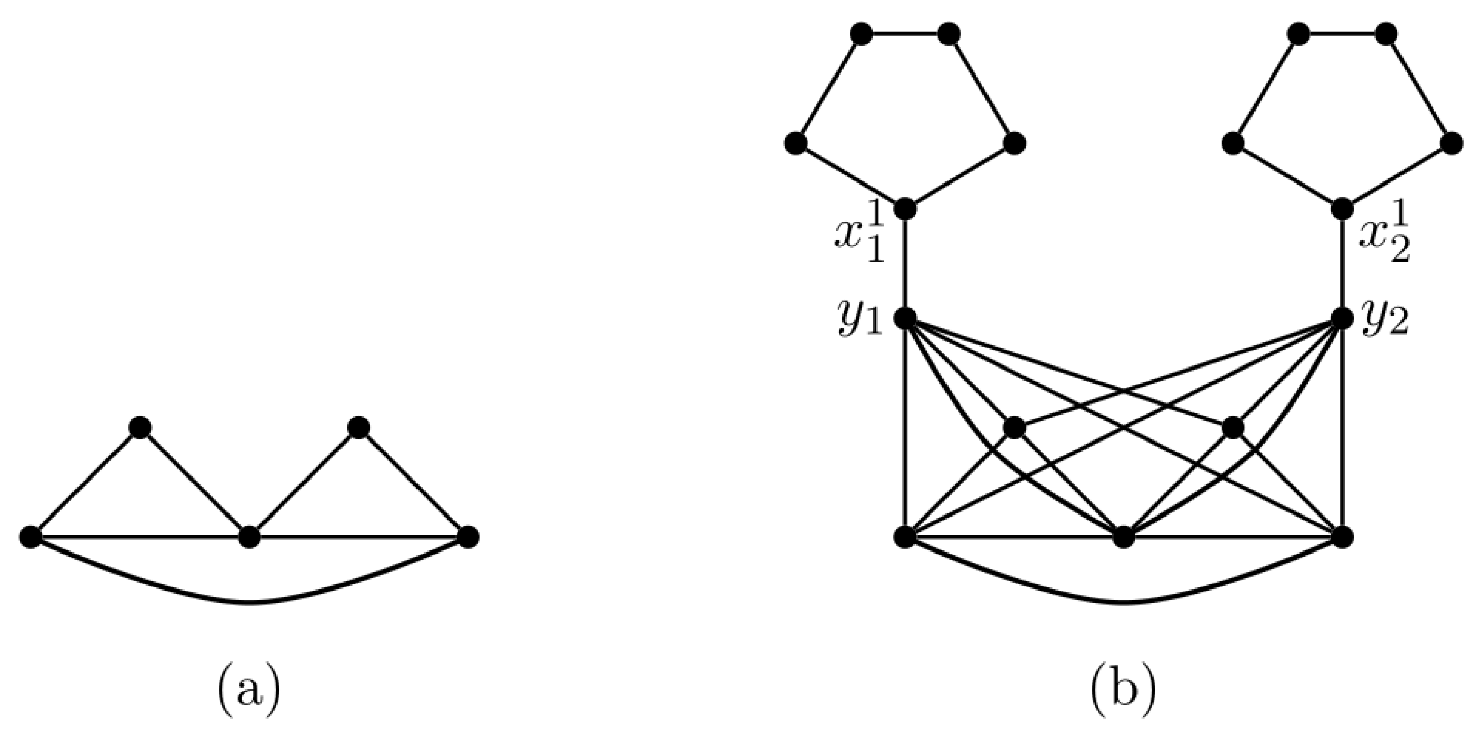
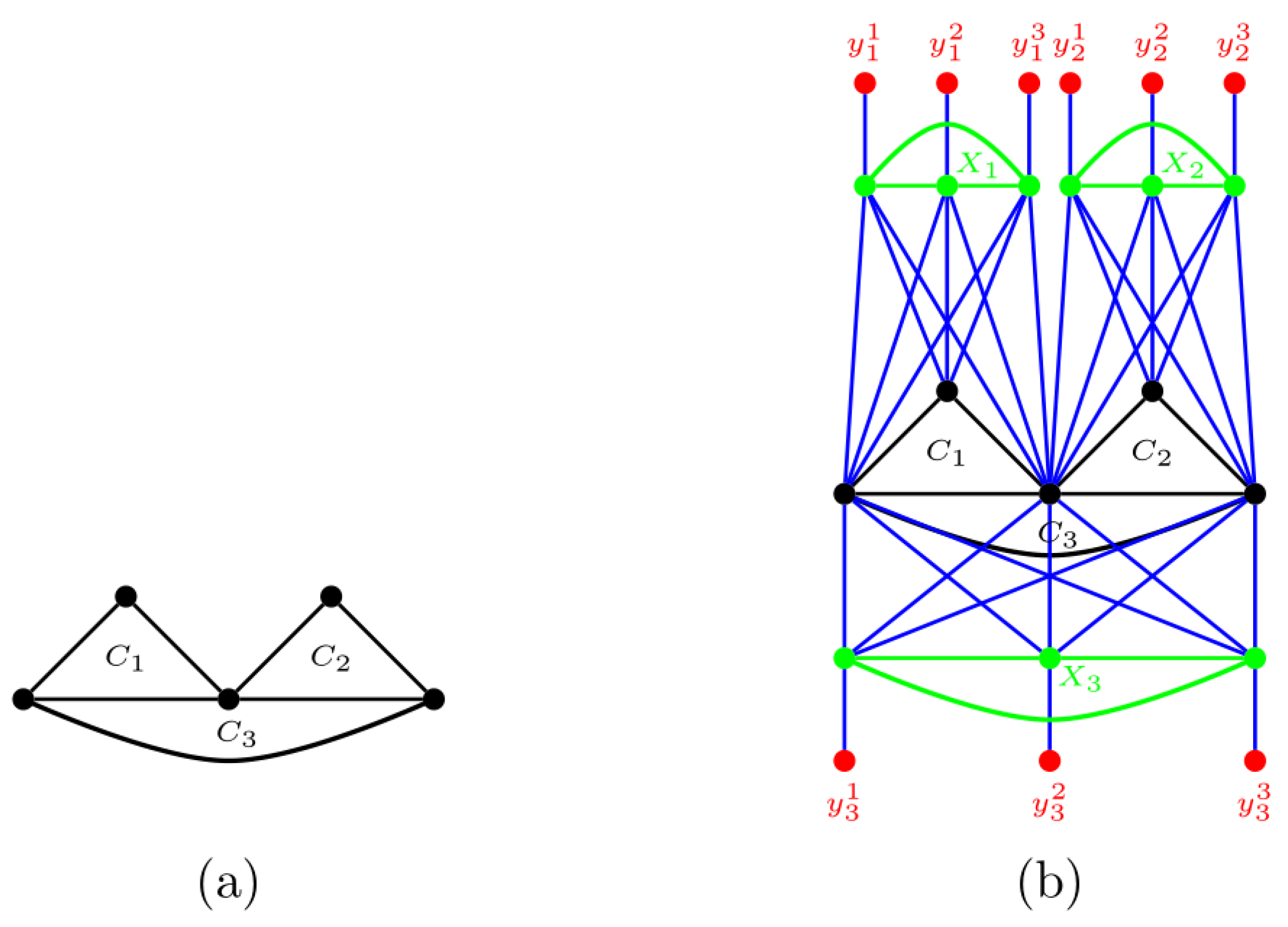
Table 1.
Previous para-NP-completeness and W[2]-completeness results on the CTP and its variants.
| Parameter: Solution Size or Weight | |||||
|---|---|---|---|---|---|
| Graphs | CTP | -FMCTP | -MCTP | SMCTP | MMCTP |
| Chordal | -c [17] | -c [13] | -c [13] | para-NP-c [17] | − |
| () | () | ||||
| Doubly Chordal | − | − | − | para-NP-c [17] | − |
| Split | -c [17] | − | − | − | − |
| Planar | − | − | − | para-NP-c [17] | para-NP-c [17] |
Table 2.
Previous FPT results on the CTP and its variants.
| Problem | Bounded Treewidth Graph | Planar Graph |
|---|---|---|
| Parameter: Treewidth k | Parameter: Solution Size or Weight k | |
| CTP | [18] | − |
| MCTP | [17] | [13] |
| d-FMCTP | [17] | − |
| -MCTP | [17] | − |
| SMCTP | [17] | − |
| MMCTP | [17] | − |
Table 3.
Our para-NP-completeness and W[2]-completeness results on the CTP variants.
| Parameter: Solution Size or Weight | ||||
|---|---|---|---|---|
| Graphs | -FCTP | -CTP | SCTP | MCTP |
| Chordal | -c | − | -c | -c |
| Doubly Chordal | -c | − | para-NP-c | − |
| Split | -c | − | para-NP-c | para-NP-c |
| Planar | − | − | para-NP-c | para-NP-c |
| − | W[2]-c | − | − | |
Table 4.
Our FPT results on the CTP and its variants.
| Problem | Bounded Treewidth Graph | Planar Graph |
|---|---|---|
| Parameter: Treewidth k | Parameter: Solution Size or Weight k | |
| 1-FCTP | ||
| d-FCTP (, 3) | ||
| d-FCTP () | (Note: ) | |
| d-FCTP () | None (Note: .) | |
| -CTP | ||
| SCTP | (Note: .) | |
| MCTP | (Note: It holds for .) |
Disclaimer/Publisher’s Note: The statements, opinions and data contained in all publications are solely those of the individual author(s) and contributor(s) and not of MDPI and/or the editor(s). MDPI and/or the editor(s) disclaim responsibility for any injury to people or property resulting from any ideas, methods, instructions or products referred to in the content. |
© 2023 by the author. Licensee MDPI, Basel, Switzerland. This article is an open access article distributed under the terms and conditions of the Creative Commons Attribution (CC BY) license (https://creativecommons.org/licenses/by/4.0/).
Share and Cite
MDPI and ACS Style
Lee, C.-M. Clique Transversal Variants on Graphs: A Parameterized-Complexity Perspective. Mathematics 2023, 11, 3325. https://doi.org/10.3390/math11153325
AMA Style
Lee C-M. Clique Transversal Variants on Graphs: A Parameterized-Complexity Perspective. Mathematics. 2023; 11(15):3325. https://doi.org/10.3390/math11153325
Chicago/Turabian StyleLee, Chuan-Min. 2023. "Clique Transversal Variants on Graphs: A Parameterized-Complexity Perspective" Mathematics 11, no. 15: 3325. https://doi.org/10.3390/math11153325
Note that from the first issue of 2016, this journal uses article numbers instead of page numbers. See further details here.