

COVID-19: From Limit Cycle to Stable Focus

1
Institute for Information Transmission Problems of RAS (Kharkevich Institute), Bolshoy Karetny per. 19, Build. 1, Moscow 127051, Russia
2
Vernadsky Institute of Geochemistry and Analytical Chemistry of RAS, Kosygin Street 19, Moscow 119991, Russia
*
Author to whom correspondence should be addressed.
Mathematics 2023, 11(14), 3226; https://doi.org/10.3390/math11143226
Submission received: 27 June 2023
/
Revised: 17 July 2023
/
Accepted: 19 July 2023
/
Published: 22 July 2023
(This article belongs to the Special Issue Advances in the Mathematics of Ecological Modelling)
Abstract
:The study aims at investigating a new fundamental property of infectious diseases with natural adaptive immunity that weakens over time—qualitative change (bifurcation) in the behavior of the “virus vs. human” system with an increase in contagiousness. Numerical experiments with a model of the COVID-19 epidemic in Moscow have demonstrated that when the reproduction number R0 is about 4, a qualitative change (bifurcation) occurs in the behavior of the virus–human system. Below this value, the long-term forecast tends toward undamped oscillations; above it, the forecast shows damped oscillations: the amplitudes of epidemic waves decrease gradually, with a constant, very high background level of morbidity that keeps natural immunity near 100%. To confirm this result analytically, we use an original modification of the Euler–Lotka renewal equation, which describes the dynamics of infected patients distributed by disease duration (time since infection) and accounts for immunity. To construct a bifurcation diagram, which illustrates the dependence of the equilibrium stability on the parameter R0, we linearize the equation in the vicinity of the equilibrium point and examine its numerical approximation (discrete form). This approximation can be interpreted as a Leslie model, with the matrix elements dependent on the parameter R0. By examining the roots of the corresponding Lotka polynomial, we can assess the stability of the equilibrium point and verify the basic assumption about the change in the properties of the system with increasing R0—about the transition from undamped oscillations to damped ones. For the bifurcation diagram, we use the functions obtained from the simulation of the COVID-19 epidemic in Moscow. However, observations of the epidemic in other cities and countries support the primary finding of our study regarding the attenuation of epidemic waves.
MSC:
92D301. Introduction
The growing application of population models in assessing the dynamics of real biological objects necessitates greater accuracy and detail in the description. Simple models, in which individuals are considered to be identical, are replaced by models with the internal structure of a population, where individuals may differ in the values of various parameters [1,2]. Distributed models are of particular interest. In this case, the population structure is determined by the distribution of individuals along a continuous parameter, for example, height, weight, position in space, age, etc.
The use of models with an age structure allows for a more detailed and accurate description of the behavior of a population in cases where the parameters that determine its dynamics depend significantly on age. Here, the “age” can mean various indicators that change over time: time since birth (demography and population dynamics) [1,2,3,4], time since the infection (epidemiology, including immunity dynamics) [4,5,6], time since cell division (tissue growth) [7], etc.
Population models with an age structure allow us to explain phenomena such as demographic (population) waves [8], to consider the dynamics of immunity [5,6], and to formalize the relationship between rates of evolution and rates of environmental change [9]. This enhances expressiveness of the models, increases potential accuracy in describing natural phenomena, and improves understanding of the laws of their functioning.
Results obtained via this approach exemplify its efficiency. In this study, we begin by presenting some statistics and results of using the simulation model of the COVID-19 epidemic in Moscow (Moscow selected as an example). Subsequently, we propose a hypothesis about changing the long-term behavior of the system. Finally we introduce and explore an original mathematical model of the virus–human system explaining that behavior.
2. Materials and Methods
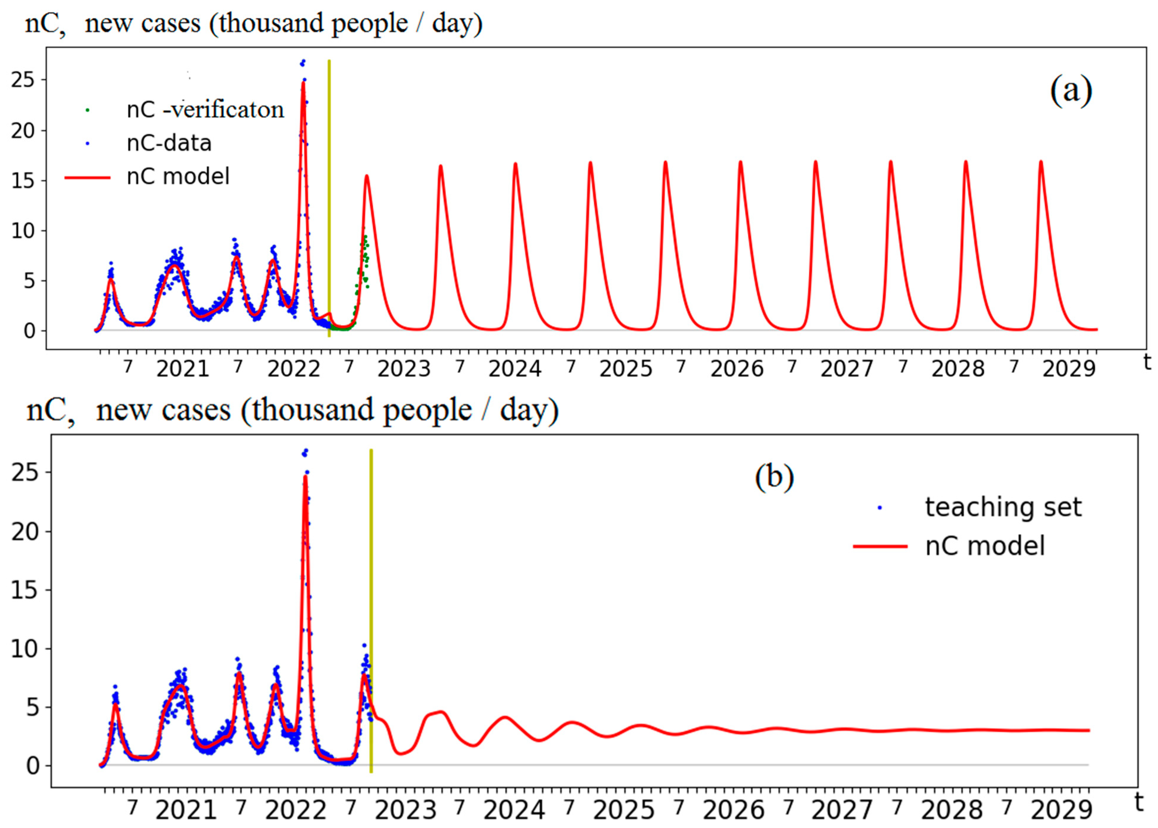
Figure 1 shows forecasts (from 27 April 2022 and 6 September 2022) of new detected cases (nC), obtained via the simulation model [5,6] and identified via the real data collected in Moscow. The detailed model used describes the dynamics of infected people, distributed over the time of illness, taking into account immunity, contact restrictions, isolation of patients, vaccination, and migration. For identification, statistical data on the number of detected infected (new cases), the number of tests, the number of antibody carriers, and vaccinations are used. In Figure 1a, the dynamics enter the mode of undamped oscillations with a period of about 8 months and with a maximum of about 15,000 cases. In Figure 1b, the dynamics display the mode of damped oscillations around a (background) value of 3500 cases and with a period of about 7 months; the amplitude of each wave is lower by 30% than the previous one.
The main parameter determining the qualitative difference in the forecasts dynamics is the reproduction number R0: In the first forecast R0 = 2.7 and in the second one R0 = 15.6.
Therefore, variations in the contagiousness of a virus result in a qualitative change in the virus–human system’s behavior.
The presented numerical experiments inspire a more complete study of the model used: the definition of stationary states and limit cycles and their stability depending on the critical (bifurcation) parameter R0, i.e., the construction of the bifurcation diagram of the system.
The complete complex model [5,6] takes into account various factors such as testing rate, vaccination intensity, herd immunity, etc. It can be regarded as a modification of McKendrick–Von Foerster model [2,4] or Leslie model [2,3] or as a mixed Cauchy problem for the transport equation [10,11] with a specific boundary condition (representing the emergence of new infected).
To conduct a mathematical study, we use a simplified model (everything was removed, except for contagiousness and immunity, depending on the time of the infection).
where I(t,a) is the number of infected with infection duration (the number of days since the moment of infection) a at time t, I0(a)—the number of infected people at the initial moment t = 0 (initial condition), B(t)—the number of new infected (a = 0) at time t (boundary condition), R0—the reproduction number, Imm(t)—the proportion of the population with immunity (at time t), A—the maximum duration of the disease (14 days), b(a)—the normalized (integral equal to 1) contagiousness as a function of disease duration a, N—population size, I—the maximum duration of immunity period (270 days), fImm(t)—proportion of infected who maintained immunity t days after the disease.
By integrating the first equation along the characteristic (a = t + Const), we obtain the number of infected with infection duration a at time t as the number of new infected at time t − a:
which leads to a modified (accounting for immunity) Euler–Lotka renewal integral equation [2,7,12]:
or by combining both equations:
Equation (1) describes the emergence of new infected as the product of the reproduction number R0 (how many people a sick person can infect), the proportion of the population without immunity (1 − Im(t)), and the total number of infected, weighted by taking into account the dependence of contagiousness on disease duration. Equation (2) describes the proportion of carriers of natural immunity as the number of infected people who have retained immunity until time t, divided by the total population N.
To find a stationary solution (equilibrium position), we substitute B(t) = B0 and Imm(t) = Imm0 into Equations (1) and (2) and obtain:
To study its stability, we linearize Equation (3) near the equilibrium point Equation (4):
and, neglecting the values of the 2nd order and higher, we obtain a linear integral equation:
where
(Here the function b(t) is extended by zero values for t > A).
B(t) = B0+ Δ(t)
Integral Equation (5) is linear. The analysis of its stability is based on the study of eigenvalues and functions [2,7,12]. Therefore, we will look for a solution in the form As a result, we obtain an eigenvalue problem—the Lotka equation:
The roots of Equation (7) allow us to judge the stability of equilibrium Equation (4) of Equation (3). If, for all solutions r of Equation (7), Re(r) < 0, then Δ(t) tends toward 0 and the equilibrium position Equation (4) of Equation (3) (or system (1)–(2)) is stable. Otherwise, if there exists r with Re(r) > 0, the equilibrium is unstable. Thus, we can determine the stability of stationary solutions depending on the value of the (bifurcation) parameter R0.
The considered eigenvalue problem Equation (7) has no analytical solutions, so it is natural to study its discrete numerical approximation:
Note. Equation (8) can be converted to the characteristic equation in the following form:
where λ = er.
It has been established [2,3] that the obtained polynomial is the characteristic polynomial of the Leslie matrix (corresponding to problem Equation (5)). However, unlike the classical setting, the function Φ(t, R0) and the corresponding elements of the Leslie matrix can take negative value. Therefore, we should not expect the dominant eigenvalue to be real.
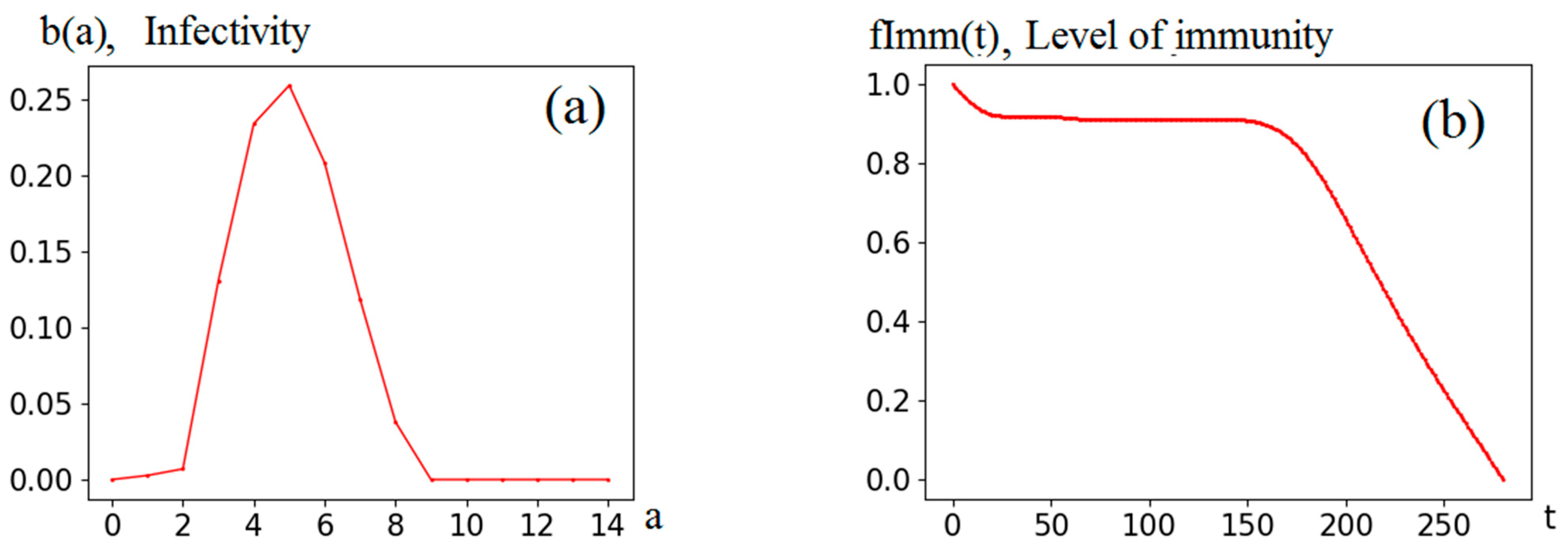
The following calculations are based on the functions (see Figure 2) that were obtained earlier when identifying the comprehensive model [5,6] for the COVID-19 epidemic in Moscow. They are used to calculate Φ(t, R0) and corresponding elements of the numerical model (8). It is these functions, together with the parameter R0, that determine system behavior.
3. Numerical Results and Discussion
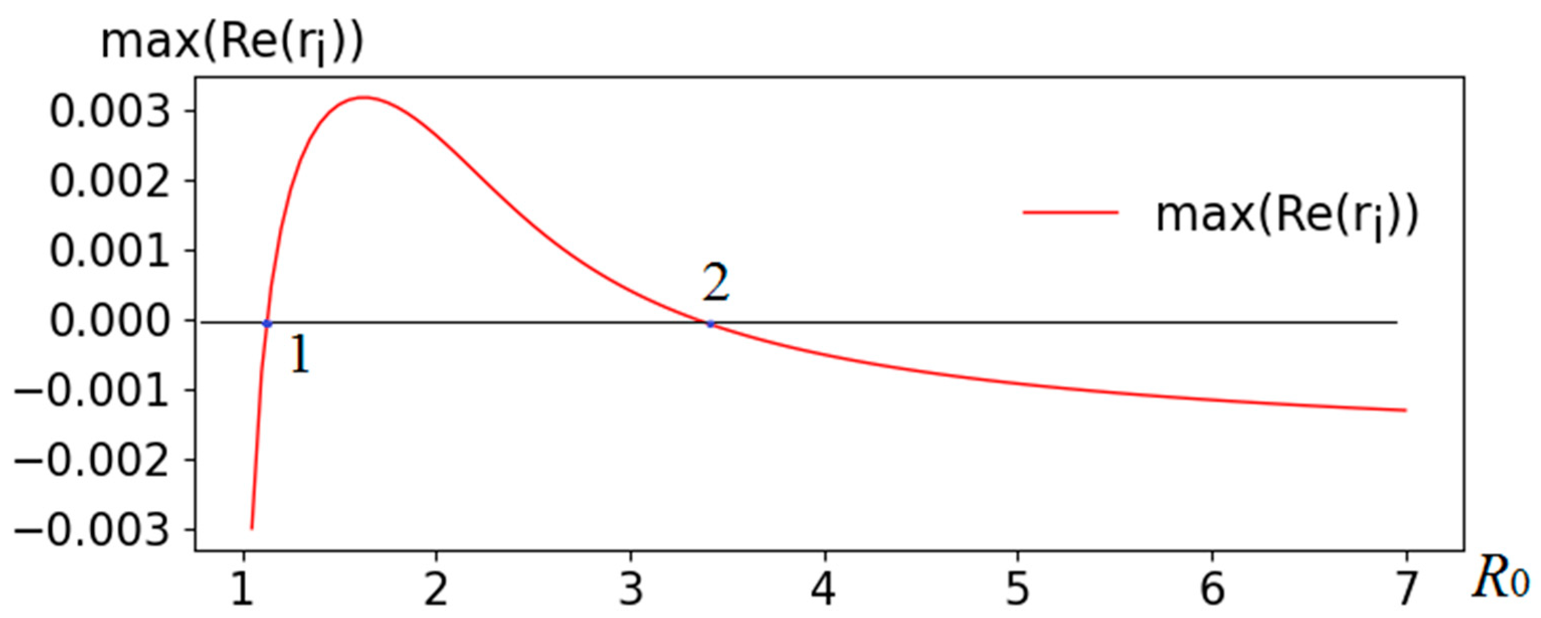
Figure 3 shows the results of a numerical study of the eigenvalue problem Equation (8). Bifurcation points (change of sign) are marked “1” (R0 value about 1.16) and “2” (R0 value about 3.5). Thus, we obtain three areas: to the left of point 1, the equilibrium Equation (4) of system (1)–(2) is stable; between points 1 and 2, it is unstable; and to the right of 2, the equilibrium is stable.
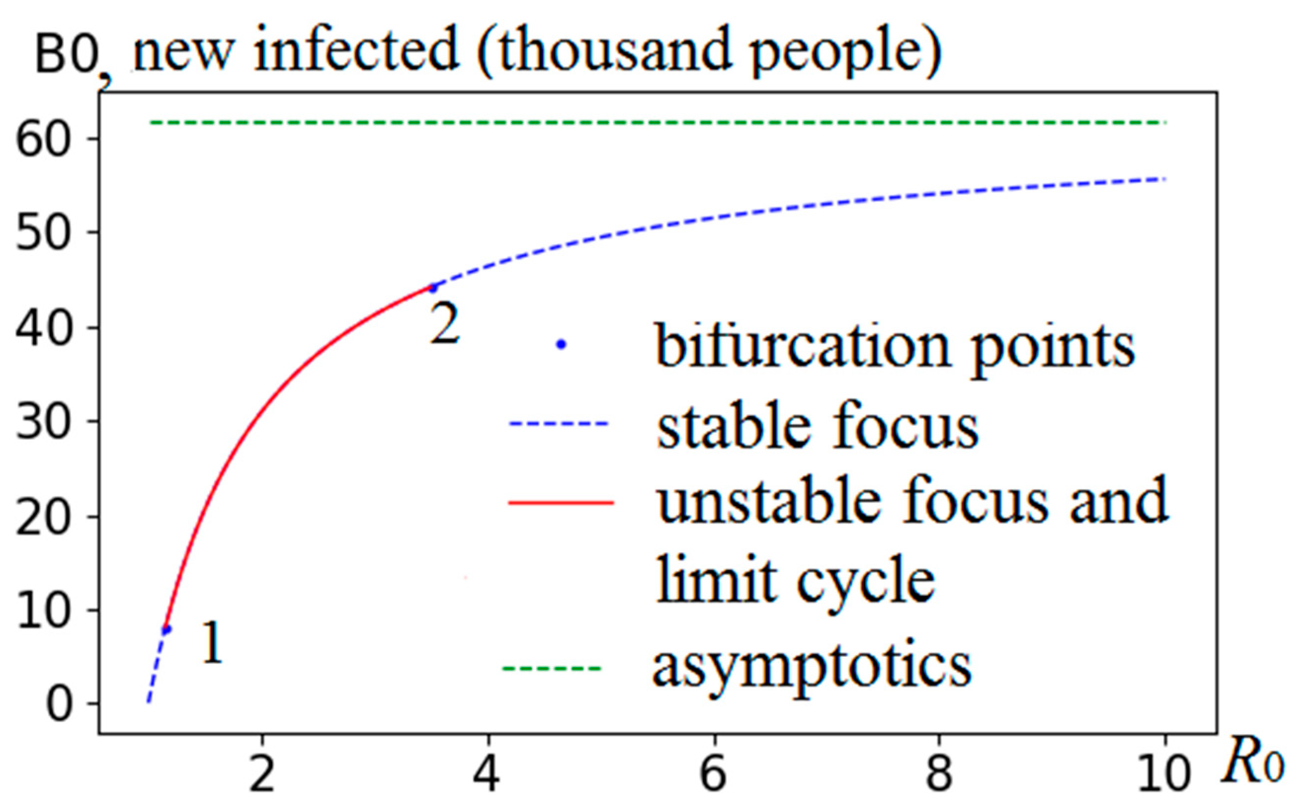
Another representation of the results in the form of a bifurcation diagram (in the space B0 × R0) is shown in Figure 4. As R0 increases, at point 1, a stable focus is transformed into an unstable focus. At point 2, the reverse transformation occurs—an unstable focus passes into a stable focus. With a further increase in R0, the equilibrium position (stable focus) asymptotically tends toward the final limit (asymptotics in Figure 4).
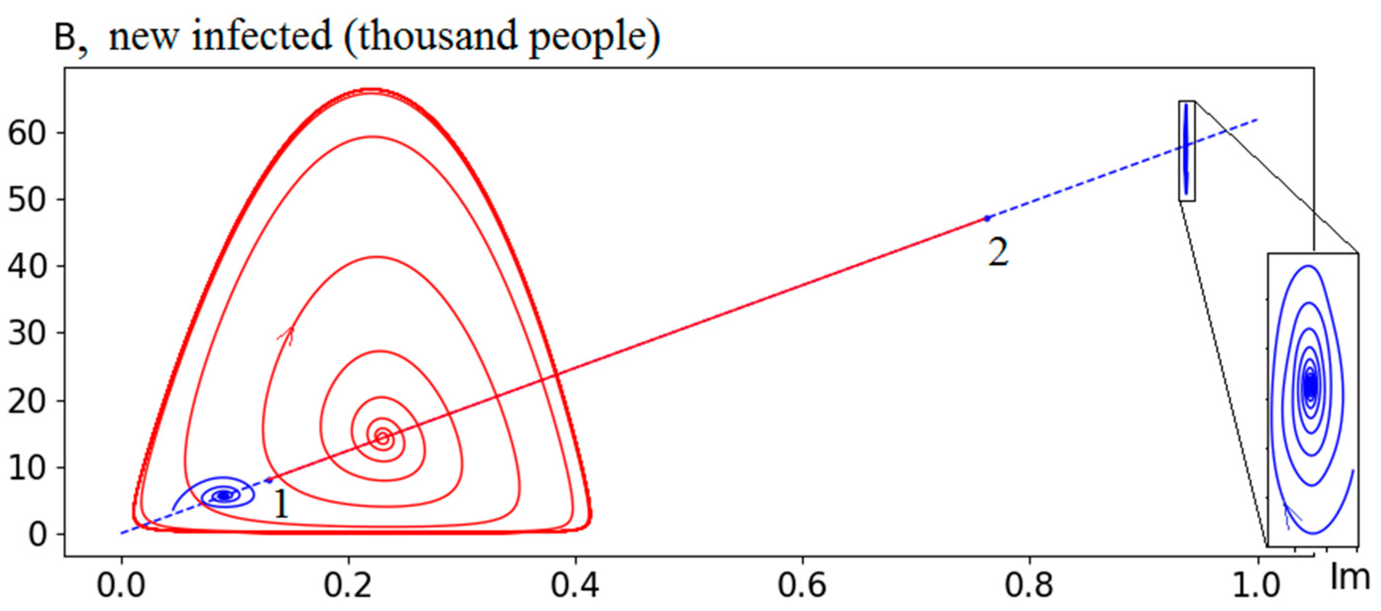
Figure 5 provides a more visual representation in the phase space B × Im. In addition to the equilibrium points from Equation (4), the figure shows some trajectories and limit cycles calculated on the basis of the numerical approximation of the model (1)–(2).
Figure 5 shows the phase portrait of system (1)–(2). The left point of the straight line with coordinates (0,0) corresponds to R0 ≤ 1 (the epidemic ends). Further, the straight line up to bifurcation point 1 (R0 value is about 1.16) corresponds to a stable focus. The displayed trajectory example (blue stable focus on the left part) corresponds to the value R0 = 1.1. At bifurcation point 1, a qualitative change occurs in the system’s dynamic properties—the focus becomes unstable and a stable limit cycle appears (calculated from model (1)–(2), as the linearized model (5) is not sufficient). The given trajectory example (in the limit, a red stable cycle) corresponds to R0 = 1.3. As we approach point 2, the cycle amplitude initially increases (for example, at R0 = 3, amplitude B reaches 700 thousand), and then begins to decrease (at R0 = 3.6, amplitude B is about 80 thousand). The cycle also becomes more complex (with self-intersections), and closer to point 2, the system’s motion possibly becomes chaotic (this statement requires further research). After bifurcation point 2, the system’s behavior is once again described by a stable focus. The example shown (blue stable focus on the right) corresponds to R0 = 16.
Let us draw some practical conclusions from this analysis.
At large values of R0, the system tends toward a stable equilibrium point. The level of immunity at this point is determined (according to Equation (4)) by the formula (R0 − 1)/R0·100%. For instance, if the reproduction number R0 = 10, then for zero growth, 9 of 10 people must be immune. With R0 more than 10, stationary solutions do not differ much from each other (see Figure 4)—more than 90% of the population should have natural immunity. Therefore, according to the model considered, the emergence of more infectious strains does not significantly alter the situation.
4. Conclusions
Numerical experiments with the COVID-19 simulation model in Moscow [5,6] have led us to propose a hypothesis about a qualitative change in the behavior of the “virus vs. human” system as virus contagion increases. Mathematical study of the corresponding reduced model (1)–(2) confirmed this assumption. The critical value of the reproduction number R0 is about 3.5. Below this value (observed until 2022), the forecast tends toward undamped oscillations (stable limit cycle). Above this value, it is described by damped fluctuations (stable focus), with decreasing amplitudes of epidemic waves and a constant, very high background level of morbidity that maintains natural immunity slightly below 100%. For the current situation in Moscow (as of May 2023), according to the model, the wave period is about 7 months and the amplitude of each wave is 30% lower than the previous one. These values align with the current situation quite well.
The above calculations are approximate. They are based on functions obtained earlier in the identification of the full model [5,6] for the COVID-19 epidemic in Moscow. Moscow and the COVID-19 epidemic have been chosen as a well-documented example. Similar calculations can be conducted for other populations and diseases.
The theoretical results obtained are of a fundamental (general) nature. They were obtained from a simplified model that takes into account only contagiousness and immunity retention (as functions of time since infection). The effects found are present in all epidemics of infectious diseases with natural adaptive immunity weakening over time, although they can be masked by other stronger factors, such as contact restrictions, vaccination, migration, seasonality, etc.
We can hope that our immune system will learn to “remember” the contact with the virus for a longer time (as of now, according to calculations [5,6], about 200 days), and then the “tribute” to maintain immunity will become significantly less. Another hope for combating infectious diseases is the emergence of newer, more effective vaccines.
Author Contributions
Conceptualization, A.S.; methodology, A.S.; software, A.S. and V.V.; validation, A.S. and V.V.; formal analysis, A.S. and V.V.; investigation, A.S. and V.V.; writing—original draft preparation, A.S. and V.V.; writing—review and editing, A.S. and V.V.; supervision, A.S.; project administration, V.V. All authors have read and agreed to the published version of the manuscript.
Funding
This work was supported by the Russian Science Foundation under grant no. 22-11-00317, https://rscf.ru/project/22-11-00317/ (accessed on 21 June 2023).
Acknowledgments
This work has been carried out using computing resources from the federal collective usage center Complex for Simulation and Data Processing for Megascience Facilities at NRC “Kurchatov Institute”.
Conflicts of Interest
The authors declare no conflict of interest. The funders had no role in the design of the study; in the collection, analyses, or interpretation of data; in the writing of the manuscript; or in the decision to publish the results.
References
- Logofet, D.O.; Ulanova, N.G. From Population Monitoring to a Mathematical Model: A New Paradigm of Population Research. Biol. Bull. Rev. 2022, 12, 279–303. [Google Scholar] [CrossRef]
- Caswell, H. Matrix Population Models: Construction, Analysis, and Interpretation, 2nd ed.; Sinauer Associates: Sunderland, MA, USA, 2001; 722p. [Google Scholar]
- Leslie, P.H. On the use of matrices in certain population mathematics. Biometrika 1945, 33, 183–212. [Google Scholar] [CrossRef] [PubMed]
- Keyfitz, B.L.; Keyfitz, N. The McKendrick partial equation and its uses in epidemiology and population studies. Math. Comput. Model. 1997, 26, 1–9. [Google Scholar] [CrossRef]
- Sokolov, A.; Sokolova, L. Monitoring and forecasting the COVID-19 epidemic in Moscow: Model selection by balanced identification technology—Version: September 2021. medRxiv 2021. [Google Scholar] [CrossRef]
- Sokolov, A.V.; Sokolova, L.A. Monitoring and prediction of COVID-19 morbidity dynamics in Moscow: 2020–2021. Epidemiol. Vaccinal Prev. 2021, 21, 48–59. [Google Scholar] [CrossRef]
- Akimenko, V.V.; Adi-Kusumo, F. Age-structured Delayed SIPCV Epidemic Model of HPV and Cervical Cancer Cells Dynamics II. Convergence of Numerical Solution. Biomath 2022, 11, 1–20. [Google Scholar] [CrossRef]
- Chen, Y.; Huang, Y. The power of the government: China’s Family Planning Leading Group and the fertility decline of the 1970s. Demogr. Res. 2020, 42, 985–1038. [Google Scholar] [CrossRef]
- Sokolov, A.V. Mechanisms of Regulation of the Speed of Evolution: The Population Level. Biophysics 2016, 61, 513–520. [Google Scholar] [CrossRef]
- Bagrov, V.G.; Belov, V.V.; Zadorozhnyi, V.N.; Trifonov, A.Y. Methods of Mathematical Physics. Special Functions. Equations of Mathematical Physics; TPU Publishing House: Tomsk, Russia, 2012; 257p. [Google Scholar]
- Zeldovich, Y.B.; Myshkis, A.D. Elements of Mathematical Physics. Medium of Non-interacting Particles; FIZMATLIT: Moscow, Russia, 2008; 368p. [Google Scholar]
- Kot, M. The Lotka integral equation. In Elements of Mathematical Ecology; Cambridge University Press: Cambridge, UK, 2001; pp. 353–364. [Google Scholar]
Figure 1.
Long-term forecasts of the COVID-19 epidemic in Moscow: (a) the forecast from 27 April 2022 with a reproduction number R0 = 2.7; (b) the forecast from 6 September 2022 with reproduction number R0 = 15.6. The t-axis has marks corresponding to months and years. The vertical yellow line corresponds to the forecast start date. The model curves (red) identified on the training data set (blue dots) can be compared to the test set (green dots in panel (a)).

Figure 2.
Functions defining the dynamics of the model (1)–(2): (a) normalized (with integral equal to one) infectivity (contagiousness) as a function of time since infection (days). (b) Immunity level (1 corresponds to 100%) as a function of time since infection (days).
Figure 2.
Functions defining the dynamics of the model (1)–(2): (a) normalized (with integral equal to one) infectivity (contagiousness) as a function of time since infection (days). (b) Immunity level (1 corresponds to 100%) as a function of time since infection (days).

Figure 3.
Results of the numerical study of the eigenvalue problem. Sign inversion points are marked 1 and 2.
Figure 3.
Results of the numerical study of the eigenvalue problem. Sign inversion points are marked 1 and 2.

Figure 4.
Bifurcation diagram: point 1—loss of stability, point 2—transition to stability.

Figure 5.
Phase portrait of the system (1)–(2): 1 and 2 are bifurcation points, stable focuses are blue, unstable focus and stable limit cycle are red.
Figure 5.
Phase portrait of the system (1)–(2): 1 and 2 are bifurcation points, stable focuses are blue, unstable focus and stable limit cycle are red.

Disclaimer/Publisher’s Note: The statements, opinions and data contained in all publications are solely those of the individual author(s) and contributor(s) and not of MDPI and/or the editor(s). MDPI and/or the editor(s) disclaim responsibility for any injury to people or property resulting from any ideas, methods, instructions or products referred to in the content. |
© 2023 by the authors. Licensee MDPI, Basel, Switzerland. This article is an open access article distributed under the terms and conditions of the Creative Commons Attribution (CC BY) license (https://creativecommons.org/licenses/by/4.0/).
Share and Cite
MDPI and ACS Style
Sokolov, A.; Voloshinov, V. COVID-19: From Limit Cycle to Stable Focus. Mathematics 2023, 11, 3226. https://doi.org/10.3390/math11143226
AMA Style
Sokolov A, Voloshinov V. COVID-19: From Limit Cycle to Stable Focus. Mathematics. 2023; 11(14):3226. https://doi.org/10.3390/math11143226
Chicago/Turabian StyleSokolov, Alexander, and Vladimir Voloshinov. 2023. "COVID-19: From Limit Cycle to Stable Focus" Mathematics 11, no. 14: 3226. https://doi.org/10.3390/math11143226
Note that from the first issue of 2016, this journal uses article numbers instead of page numbers. See further details here.