Article

An Adaptive Jellyfish Search Algorithm for Packing Items with Conflict

by
Walaa H. El-Ashmawi
1,2,†,
Ahmad Salah
3,4,*,†,
Mahmoud Bekhit
5,6,7,†,
Guoqing Xiao
8,9,
Khalil Al Ruqeishi
10 and
Ahmed Fathalla
11,*
1
Faculty of Computers and Informatics, Suez Canal University, Ismailia 41522, Egypt
2
Faculty of Computer Science, Misr International University, Cairo 44971, Egypt
3
Faculty of Computers and Informatics, Zagazig University, Sharkia 44519, Egypt
4
College of Computing and Information Sciences, University of Technology and Applied Sciences, Ibri P.O. Box 466, Oman
5
University of Technology Sydney (UTS), Sydney, NSW 2007, Australia
6
Australian Catholic University, Sydney, NSW 2059, Australia
7
Kaplan Business School, Sydney, NSW 2000, Australia
8
College of Computer Science and Electronic Engineering, Hunan University, Changsha 410082, China
9
The National Supercomputing Center in Changsha, Changsha 410082, China
10
Mathematical and Physical Sciences Department, College of Arts and Sciences, University of Nizwa, Nizwa P.O. Box 33, Oman
11
Department of Mathematics, Faculty of Science, Suez Canal University, Ismailia 41522, Egypt
*
Authors to whom correspondence should be addressed.
These authors contributed equally to this work.
Mathematics 2023, 11(14), 3219; https://doi.org/10.3390/math11143219
Submission received: 30 May 2023 / Revised: 6 July 2023 / Accepted: 8 July 2023 / Published: 22 July 2023
(This article belongs to the Topic Applied Metaheuristic Computing: 2nd Volume)

Abstract

:
The bin packing problem (BPP) is a classic combinatorial optimization problem with several variations. The BPP with conflicts (BPPCs) is not a well-investigated variation. In the BPPC, there are conditions that prevent packing some items together in the same bin. There are very limited efforts utilizing metaheuristic methods to address the BPPC. The current methods only pack the conflict items only and then start a new normal BPP for the non-conflict items; thus, there are two stages to address the BPPC. In this work, an adaption of the jellyfish metaheuristic has been proposed to solve the BPPC in one stage (i.e., packing the conflict and non-conflict items together) by defining the jellyfish operations in the context of the BPPC by proposing two solution representations. These representations frame the BPPC problem on two different levels: item-wise and bin-wise. In the item-wise solution representation, the adapted jellyfish metaheuristic updates the solutions through a set of item swaps without any preference for the bins. In the bin-wise solution representation, the metaheuristic method selects a set of bins, and then it performs the item swaps from these selected bins only. The proposed method was thoroughly benchmarked on a standard dataset and compared against the well-known PSO, Jaya, and heuristics. The obtained results revealed that the proposed methods outperformed the other comparison methods in terms of the number of bins and the average bin utilization. In addition, the proposed method achieved the lowest deviation rate from the lowest bound of the standard dataset relative to the other methods of comparison.

1. Introduction

The BPP is one of the main combinatorial optimization problems that has received much attention in the literature [1]. It is used in multiprocessor scheduling, phone call dispatching over transmission circuits, printed circuit board design, assembly line balance, and capacitated vehicle routing. The objective of the BPP is to pack a set of objects with particular sizes into a minimum number of fixed bins’ capacities. This is done in such a way that the total items’ size in a bin does not exceed the bin’s capacity. Other packing procedures involve perishable items such as medicine, food, and hazardous chemicals, some of which cannot be stored together due to their biological, chemical, or physical differences [2]. The BPP has many variations such as the 2D and 3D BPP [3,4,5].
Along with the standard form of the BPP, various variations have been investigated in the literature, including item fragmentation and specific sets of incompatible items that cannot be put together into the same bin. Item fragmentation (i.e., breaking an item into two or more parts and putting each component into a separate container) is prohibited under the basic BPP. However, in other cases, this assumption is extremly limiting. These applications include message transmission in community television networks [6], very large-scale integrated circuit design [7], file system operation [8], vehicle routing with split delivery [9], fully optical network planning [10], and the allocation of available memory to processors in parallel processing [11]. This variation of the BPP is known as the bin packing problem with item fragmentation (BPPIF). The BPPIF is a simple problem if the fragmentation is unrestricted. Several nontrivial versions of the BPPIF have been investigated by [12], including variants with various objective functions and item fragmentation constraints.
Packing a specific set of items into the same bin is not permitted in several BPP applications. This variation of the BPP is referred to as the BPP with conflicts (BPPCs). It has many applications in scheduling evaluation [13], delivery planning for any explosive, flammable, or toxic substances that cannot be packed together in the same vehicle [14], load balancing challenges in parallel computing, process assignments to processors when some processes cannot be executed on the same processor [15], and the warehouse storage of incompatible goods (such as explosive and flammable items) [16]. When developing a viable solution, it is necessary to consider conflict elimination [17] and dense packing [18] concurrently in order to achieve global optimization.
Consequently, the authors of [15] first utilized the graph theory method to characterize the conflict connection and then developed a steady approximation algorithm by periodically finding the largest induced subgraph. In [19], the authors studied the BPPCs issue using a set cover-based approach and presented an exact branch-and-bound technique based on approximate estimates of the bottom limits. The authors of [20] defined and developed an integer programming paradigm, as well as discussed the problem’s bottom limits. Elhedhli et al. [21] solved the BPPC by considering conflict constraints issues by establishing branch criteria and by applying the dynamic programming method. Khanafer [22] created a generic framework for solving the BPPCs based on the tree decomposition technique. Apart from the preceding, the BPPCs model was used to solve scheduling problems and resource assignment issues [23,24].
Standard mathematical programming or exact algorithms are severely constrained in terms of computing capability and efficiency when handling the BPPCs, which is a severely NP-hard issue from the standpoint of solving it [25]. These limited research works, which addressed the BPPCs using metaheuristic-based methods, have motivated the current work to investigate the BPPCs using the metaheuristic-based approach. The main contribution of this work is as follows:
  • To our knowledge, the BPPCs problem has not been addressed in the literature as one problem. The existing methods pack the conflict items first and then the non-conflict items as a separate problem. This investigation of packing all the conflict and non-conflict items at one stage is the first of its kind.
  • To address the BPPCs, we proposed to utilize the first adapted jellyfish algorithm. The proposed work is provided as an open source code on a GitHub repository (https://github.com/Ahmed-Fathalla/An-Adaptive-Jellyfish-Search-Algorithm-for-Packing-Items-with-Conflict, accessed on 1 June 2023).
  • Two solution representation methods have been provided at different levels. Subsequently, a comparison was drawn to answer the question as to whether it is better to represent the BPPCs solution at the item level or bin level.
  • The proposed methods were evaluated on a standard dataset with different levels of problem difficulties.
The structure of this paper is organized as follows. The recent related works for the BPPCs are reviewed in Section 2. Defining the BPPCs in formal terms and proposing the main objective, as well as different constraints to solve it, are discussed in Section 3. The standard jellyfish algorithm and the proposed adaptive jellyfish algorithm for solving the BPPCs are detailed in Section 4. In Section 5. The proposed method is evaluated using two popular metaheuristics, and the utilized heuristics’ performance results are assessed on a real dataset. Section 6 concludes the main points in the paper.

2. Literature Review

This section summarizes the published research on the BPP and its variants that is relevant to our research. The scientific literature is replete with references to the BPP [26,27]. The BPP problem limitations can be classified into two types: (1) capacity constraint and (2) conflict constraint. Each constraint class generates an NP-hard subproblem on its own (i.e., bin packing or vertex coloring). Additionally, it is noteworthy that the majority of the research on the BPPCs has focused on approximation methods and mathematical programming approaches [28]. Mathematical programming has proven to be effective regarding the BPPCs, because decomposition techniques such as branch-and-price [16,19,21] are extremely efficient in the case of problems with few elements per bin. These studies explain the price problem using various branching rules, sub-procedures of the problem, and beginning columns. If the conflicts create an interval graph, the pricing issue may be effectively addressed using dynamic programming [16], although branch-and-bound approaches can be utilized in more general scenarios. These identical approaches can solve a large number of benchmark instances, up to 1000, in certain circumstances. Unfortunately, these exact methods are insufficient for several BPPCs applications, including those where the computing cost varies significantly between the instances and large-scale task allocation issues [24], including tens or hundreds of thousands of items. In other words, the larger the number of items and constraints of the BPP, the more the complexity there is for the problem, which also entails more required computing time.
Along with well-known performance-guaranteed approximation techniques, including First-Fit Decreasing (FFD), Worst-Fit Decreasing (WFD), and Best-Fit Decreasing (BFD) [14,29,30], many authors have proposed a basic (i.e., exact) method using different formulations to address the BPP and BPPCs problems (i.e., BPPCs are the main subject of this paper). For instance, the authors in [31] constructed a branch-and-bound algorithm based on an FFD branching approach by utilizing a polynomial formulation and reduction techniques. Similarly, Scholl et al. [32] constructed an exact method by combining multiple limits, reduction techniques, and a branch-and-bound procedure with a novel branching strategy. Delorme et al. [27] published a review of mathematical models and exact methods that have been created for the BPP. The authors in [33] extended this formulation to address a variety of cutting and packing challenges. The authors of [34] proposed and implemented a pseudopolynomial arc-flow formulation in a branch-and-price method. Moreover, researchers have focused their efforts on establishing a strict lower bound, as presented in [35].
Furthermore, several authors have implemented classical heuristic algorithms [36,37,38]. To this point, metaheuristics algorithms have received less attention than mathematical programming techniques for solving the BPPCs. Fernandes Muritiba et al. [19] developed an enhanced population-based metaheuristic for generating appropriate upper limits and starting columns. The approach is a sophisticated mix of a genetic algorithm utilizing the crossover operator proposed in [39] and a tabu search based on impasse class neighborhoods in [40]. Sadykov and Vanderbeck [16] presented a heuristic technique built on a supervised partial exploration of the branch-and-price search tree. It was a reasonable compromise between the exact solution and heuristics techniques. It merged the advantages of mathematical programming with a lower CPU time in the case of a few items per bin. In general, the metaheuristics for the BPPCs need more examination. Among the best-suggested metaheuristics for addressing the bin packing issue are the grouping genetic algorithms created by Falkenauer’s [41], which utilize a version of the perturbation of minimum bin slack (MBS) approach by Fleszar and Charalambous’s [42], as well as a grouping genetic algorithm with regulated gene transmission [43].
Although these algorithms considered different solutions for the BPP or BPPCs as an approximate method with lower bounds, none of them have addressed the problem of conflict items, along with the free items, as a whole. Table 1 lists a comparison between different conducted research works. The table shows that most of the work that utilized the metaheuristic approaches addressed different variations of the BPP, with less focus on the BPPCs. Therefore, this paper presents an adaptive optimization algorithm for achieving a solution to the BPPCs.

3. Problem Formulation

In this section, we identify the BPPCs as an optimization problem with a set of constraints. In addition, the problem is presented through modeling in graph theory language. To that end, after a brief introduction to the BPPCs, the mathematical model of the BPPCs problem is formulated.

3.1. Description of the Problem

In order to solve the BPPCs model, two phases should be considered: conflict exclusion and bin packing. In the conflict exclusion phase, we may utilize two graph representation approaches to express the conflict connections among the items. First, a compatible graph is designed to represent the consistent relations between the items, where the edge set describes the compatible relationships between the vertices, and the vertex set defines the item collection. Second, a conflict graph is formulated to determine the conflict connections between the items, where the edge set describes the conflict associations between the vertices, and the vertex set defines the item collection.
In the conflict graph, the BPPC items are represented by the graph’s vertices, while the graph’s edges represent the conflicts between them. Hence, the conflict elimination procedure may be readily translated into the grouping operations of the conflict graph’s nodes. Each group can then utilize the standard bin packing techniques. The constraints with packing process capacity are the most common problems that are  encountered.

3.2. Mathematical Description of BPPCs

The BPPCs conflict graph structure represents the conflict connection between the items. It can be defined as an undirected graph structure G = ( V , E ) , where V = { 1 , 2 , , n } is a set of vertices and corresponds to the items, and E is a set of edges such that ( i , j ) E when i and j conflict and correspond to the conflicted relationship among the items. The following are the primary variables to consider while putting the packing process into action: Let I = { 1 , 2 , , n } identify the set of items and B = { 1 , 2 , , m } identify the set of bins. Also, let C define the maximum bin’s capacity and w i define the weight of each item i, where i I .
The challenge is packing a set of items into the fewest possible bins without violating the main constraints that the total items’ weight must not exceed the bin’s capacity C, and no conflict items may be packed into the same bin. Two binary variables can be used directly as follows:
y b = 1 If   bin   b   is   chosen   for   packing ;   b B 0 otherwise
x i b = 1 If   the   item   i   packed   into   the   bin   b ;   i I 0 otherwise .
Using the information provided, the BPPCs 0–1 integer programming paradigm can be identified as follows. First, the objective can be formulated as in Equation (3).
M i n b = 1 m y b .
Second, different constraints have been proposed in this model to ensure that packing items into bins is feasible and applied.
b = 1 m x i b = 1 ; i I
i = 1 n w i · x i b C y b ; b B
x i b + x j b y b ; ( i , j ) E , b B
y b { 0 , 1 } , b B
x i b { 0 , 1 } , i I , b B .
The min objective solution in Equation (3) identifies the smallest number of storage bins required to hold the items. The first constraint is represented in Equation (4); it explains that every item has a specific bin allocated to it. The second constraint, in Equation (5), states that the total weight of the packed items in each bin must not exceed the maximum capacity. The third constraint in Equation (6) explains the conflicts between the two items that make up the restrictions. The 0–1 integer variables are defined by the constraints in Equations (7) and (8). Therefore, the BPPCs is considered to be one of the NP-hard problems. An optimization algorithm is required to solve such a problem.

4. The Proposed Adaptive Jellyfish Search Algorithm

This section provides an overview of the standard jellyfish search optimizer algorithm and illustrates its main stages. Moreover, the proposed adaptive jellyfish search (AJS) algorithm for solving the BPPCs problem is described in more detail based on both of the levels of solution representation (i.e., item-wise and bin-wise).
In order to address the BPPCs using the adapted JSA, several steps need to be adopted to attain an optimal number of bins. Initially, we must initialize the jellyfish’s parameters by encompassing the upper and lower limits on the number of items, the bin capacity, and the maximum number of iterations. Subsequently, the second step involves generating the initial population, which represents two solution representations: one based on individual items and the other based on individual bins. Each solution within the population consists of a collection of packed items that are organized into bins while adhering to all the imposed constraints. Next, we evaluate each jellyfish solution by applying an objective function, which specifically includes the count of bins utilized in each solution. Moving on to the jellyfish update, we employ three operators to generate a new solution by combining two existing solutions. Finally, we iterate steps 3 and 4 until the maximum number of iterations is reached, thus aiming to identify the most favorable packing solution. The proposed method’s steps are depicted in Figure 1.

4.1. The Artificial Jellyfish Search (JS) Optimizer Algorithm

Jellyfish search is one of the recently proposed metaheuristic algorithms that emulates the behavior of jellyfish in the ocean [44]. Jellyfish contain characteristics that allow them to move freely, to drive themselves ahead, and their bottoms shut like an umbrella. Despite this, they typically float in the ocean with the tides [45]. Jellyfish may swarm when conditions are good, and a large number of jellyfish is referred to as a bloom [46,47]. Jellyfish, in particular, are slow swimmers; therefore, orienting themselves toward currents is critical to keeping blooms alive and preventing stranding [46].
Ocean currents are critical because they may aggregate jellyfish into swarms [46,48,49]. This phenomenon with the individual jellyfish’s motions within the swarm and their propensity to generate jellyfish blooms in response to ocean currents has enabled these species to emerge practically anywhere in the ocean. The amount of food available at jellyfish-visited locations varies; hence, the optimal spot is discovered when food proportions are examined. As a result, a novel algorithm has been devised that was motivated by jellyfish’s search behavior and mobility in the water.
The proposed optimization approach is composed of three idealized principles:
  • In order to travel within the swarm, jellyfish can only travel in one of two directions: with or against the ocean current. A time control system is responsible for the switching between both modes of movement.
  • Jellyfish are continuously on the move in search of food; they are often more attracted to regions where food is readily available.
  • The objective function and location indicate the food quantities discovered.

4.1.1. Moving in the Ocean Current

Due to the high concentration of nutrients in the ocean current, jellyfish are attracted to it.
The ocean current (i.e., trend) direction is determined by taking the average of all of the position vectors from each jellyfish in the ocean to the current optimal jellyfish (i.e., the one in the most advantageous position in the water column).
Equation (9) models the flow of the ocean:
trend = 1 n p o p trend i = 1 n p o p ( X * e c X i ) = X * e c X i n p o p = X * e c μ
set d f = e c μ .
As a result, the  trend is determined by the following:
trend = X * d f ,
where n p o p is the total number of jellyfish in the swarm; X * denotes the current jellyfish at the most-suited locations inside the swarm; e c denotes the attraction element; and μ is the mean position of all the jellyfish. The difference between the jellyfishs’ most acceptable position and the jellyfishs’ mean location is d f .
By assuming the normal distribution of jellyfish in all dimensions, the  d f can be computed as follows:
d f = β × rand ( 0 , 1 ) × μ ,
where e c = β × rand ( 0 , 1 ) .
Then, each jellyfish’s new position is specified by the following:
X i ( t + 1 ) = X i ( t ) + rand ( 0 , 1 ) × trend .
Equation (13) can be expressed as follows:
X i ( t + 1 ) = X i ( t ) + rand ( 0 , 1 ) × X * β × rand ( 0 , 1 ) × μ ,
where β > 0 is a distribution coefficient that is proportional to the trend’s duration. Using the findings of the vulnerability analysis performed on numerical experiments of [44], we obtain β = 3.

4.1.2. Moving inside the Swarm

Jellyfish have two types of movements in a swarm: passive (type A) and active (type B) [47,50]. When the swarm first forms, the majority of jellyfish display type A motion. They gradually demonstrate more type B movements.
Type A motion refers to jellyfish moving about in their own places, and each jellyfish’s updated location is provided by Equation (15).
X i ( t + 1 ) = X i ( t ) + γ × rand ( 0 , 1 ) × ( U b L b ) ,
where U b and L b denote the upper and lower bounds of the search space, respectively. In addition, a motion coefficient with a value γ > 0 indicates how far the jellyfish move around their locations. γ = 0.1 has been acquired from the perceptiveness study results proposed in [44]. A randomly chosen jellyfish (j) imitates type B motion, and the direction of movement is defined by a vector drawn from the jellyfish of concern (i) to the randomly selected jellyfish (j). When the amount of food available to the selected jellyfish (j) exceeds the amount of food available to the jellyfish (i) of interest, the latter moves directly toward the former; when the amount of food available to the selected jellyfish (j) is less than the amount of food available to the jellyfish (i) of interest, the latter moves directly away from the former.
As a result, each jellyfish in a swarm goes in the direction that will lead to the best food. Equations (18) and (19) model the direction of travel for a jellyfish and update its position, respectively. According to some observers [51], this movement is regarded as successfully exploiting the local search space.
step = X i ( t + 1 ) X i ( t ) ,
where
step = rand ( 0 , 1 ) × Direction
Direction = X j ( t ) X i ( t ) if f ( X i ) f ( X j ) X i ( t ) X j ( t ) if f ( X i ) < f ( X j ) ,
where f denotes an objective function associated with the place X.
Hence,
X i ( t + 1 ) = X i ( t ) + step .
A time control mechanism, c ( t ) , is used to decide the motion that will occur throughout time. In addition to controlling the type A and B movements in a swarm, c ( t ) is a randomly generated value that varies between 0 and 1 over time. It also regulates the movements of the jellyfish in the direction of an ocean current; it can be computed as follows:
c ( t ) = | ( 1 t M a x i t e r ) × ( 2 × ( rand ( 0 , 1 ) 1 ) ) | ,
where t is the current time, which is represented as the iteration number, and  M a x i t e r is an initialized parameter specifying the maximum number of iterations.

4.2. The Proposed AJS Item-Wise Level (AJS_I)

As the standard jellyfish search optimizer algorithm is designed to solve a continuous optimization problem, it cannot be used directly to solve a discrete problem. Due to the fact that the BPPCs is a discrete optimization problem, we proposed an adaptive version of the standard JS algorithm in order to achieve a solution to the BPPCs by replacing the main operators in the standard algorithm with new operators. The overall steps of the proposed AJS are illustrated below:
  • Parameters initialization: Population size p s , the iteration counter t, the maximum number of iterations t m a x , upper U b and lower L b number of items, respectively, and bin capacity C.
  • A jellyfish representation: Each individual in the population (i.e., JS) represents a solution of the BPPCs, as shown in Figure 2 as an example. This representation can be described by an n-dimensional vector of integer numbers (i.e., U b = n ), where the items and bins are identified using indices and values, respectively.
    Figure 2. A jellyfish representation.
    Figure 2. A jellyfish representation.
    Mathematics 11 03219 g002
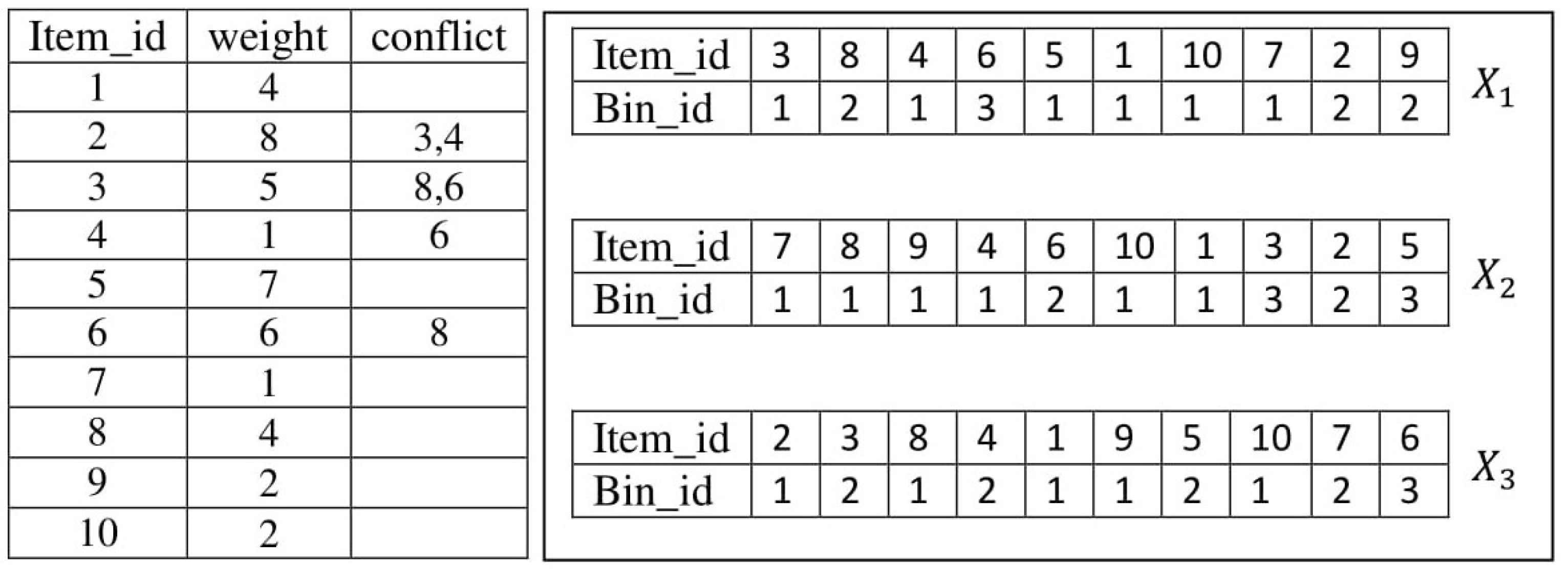
    Figure 2 represents the packing of five items into two bins. Item 1, 3, and 4 are packed into bin 1, while items 2 and 5 are packed into bin 2 according to the capacity constraint of the bins and the conflict constraint among items.
  • Initial population: Each individual X i ( i = 1 , , p s ) is generated randomly based on a specific heuristic for achieving a feasible initial solution. Figure 3 illustrates an example of the initial population of three individuals. The example consists of 10 items ( U b = 10 ) , the corresponding weight of each item, the bin capacity ( C = 20 ) , and a conflict set of items.
    Figure 3. A random initial population.
    Figure 3. A random initial population.
    Mathematics 11 03219 g003
    Each population solution X i , i = 1 , , 3 is generated by packing a collection of items into a collection of bins without violating any constraint. According to X 1 , items 3, 4, 5, 1, 10, and 7 are packed into bin 1 with a total weight of 20 and have no conflicts. Items 8, 2, and 9 are packed into bin 2, with a total weight of 14, and item 6 is packed into bin 3, with a total of 6. The initial random-based-heuristic approach guarantees feasible initial solutions to the BPPCs.
  • Individual evaluation: Each jellyfish X i is evaluated according to the fitness function f at each iteration t, and the one with the smallest fitness value is allocated to the best jellyfish X * (i.e., in the case of minimization of the objective function). In contrast, the one with the maximum fitness value is assigned to X * (i.e., in the case of the maximization of the objective function). Although minimizing the number of used bins is a primary goal of the BPP, more than one solution with different packing representations and the same total number of bins may exist. Therefore, there should be other criteria to evaluate the solution in terms of bin utility, as in Equations (21) and (22) for minimization and maximization, respectively.
    M i n i m i z e f ( X ) = 1 ( b = 1 B ( U b C ) k ) / B
    M a x i m i z e f ( X ) = b = 1 B ( U b C ) k / B ,
    where U b = l = 1 b l w l , w l is the weight of item l, b l is the number of items packed into bin b, k is an exponential factor that equals two, and and B is the number of used bins in the solution.
  • Individual update: The location of a JF is updated based on the time control mechanism c ( t ) to switch the movement between the ocean current and jellyfish swarm.
    (a)
    In the case where a jellyfish follows the ocean current, Equations (13) and (14) can be rewritten to solve the discrete BPPCs problem as follows:
    X i ( t + 1 ) = X i r a n d ( 0 , 1 ) t r e n d
    t r e n d = X * X r a n d o m ,
    where r a n d ( 0 , 1 ) is a randomly generated number, and X r a n d o m is a randomly generated jellyfish. X * , X i , and X i ( t + 1 ) represent the best jellyfish, the current one, and the updated location of X i at ( t + 1 ) , respectively.
    The new operators ⊞, ⊡, and ⊟ can be used instead of the standard operators in the JS algorithm. The operator ⊟ represents the difference between two jellyfish in the current population as a set of swaps S. Each swap s can be defined as a raw vector of three elements ( p , q , r ) , where p represents the i t e m i d , q represents the current assigned b i n i d , and r represents the new assigned b i n i d . For example, s = ( 7 , 2 , 1 ) means item 7 can be packed into bin 1 instead of bin 2. Figure 4 illustrates an example as a difference between two individuals (e.g., X 1 and X 2 ).
    Figure 4. An example of operator ⊟.
    Figure 4. An example of operator ⊟.
    Mathematics 11 03219 g004
    The ⊡ operator represents the probability of the chosen random number of swaps from the swap set S. Figure 5 illustrates an illustrative example of the results of applying the ⊡ operator. According to the example, if S has five swaps, the generated random integer number is 0.6; then, the result of ⊡ is a randomly selected set of three swaps from the set S.
    Figure 5. An example of operator ⊡.
    Figure 5. An example of operator ⊡.
    Mathematics 11 03219 g005
    The ⊞ operator takes a leading role in updating the location of a jellyfish. Therefore, it can be viewed as applying the set of swaps sequentially to the current jellyfish position in the swarm in order to obtain a new position. An illustrative example of the ⊞ operator is shown in Figure 6.
    Figure 6. An example of operator ⊞.
    Figure 6. An example of operator ⊞.
    Mathematics 11 03219 g006
    From the example in Figure 5, item 5 is currently packed into bin number one and can be swapped and packed into a new bin number three. This reassignment can be done with one condition, which is that the new packing does not violate both the capacity and conflict constraints. As for swap (5, 1, 3), the weight of item 5 should be less than or equal to the remaining capacity of bin 3, and item 5 must have no conflict with all the items in bin 3. For the second swap (6, 3, 2), the reassignment satisfies the capacity constraint but violates the conflict constraint, in which item 6 has a conflict with the items’ list in bin two according to Figure 3. In this case, to guarantee a better exploration of a new solution, we apply an Any-Fit (AF) heuristic [26]. The main idea of an AF heuristic is that, for sequential current nonempty bins (i.e., b 1 , b 2 , …, b j ), the current item will not be assigned to bin b j + 1 unless it does not fit (i.e., it violates the capacity and conflict constraint) any of the bins in the sequence b 1 , b 2 , …, b j . Therefore, item 6 tries to be packed into bin 1 and then tries to be packed into bin 2 (i.e., both bins satisfy the capacity constraint and violate the conflict constraint); then, it remains in bin 3. Item 9 can be reassigned to bin 1 instead of 2, thus satisfying both the capacity and conflict constraint. The remaining capacity and item list for both the current and new bins is updated for any reassignment that is applied.
    (b)
    In the case of a jellyfish moving inside a swarm, the individual can move according to type A (i.e., passive) or type B (i.e., active) movement based on a random number that is generated and compared to c ( t ) :
    • Type A update: The updating location of a jellyfish (JF) in a passive way can be achieved by rewriting Equation (15) as follows to solve the discrete problem:
      X i ( t + 1 ) = X i r a n d ( 0 , 1 ) γ ( U b L b ) ,
      where γ ( U b L b ) is a randomly generated integer number between L b and U b in the form of swaps in a set of S. Therefore, | S | = γ ( U b L b ) , where | S | is the cardinality of a set S. For example, if the U b = 10 and L b = 1 (i.e., the maximum and minimum number of items) and γ ( U b L b ) = 3 , then | S | = 3 . There are three randomly generated swaps in S. This modification in the operators guarantees multiple solutions through randomization. The ⊡ and ⊞ operators can be applied with the same concept as before.
    • Type B update: This involves updating the current location of an actively based JF on a randomly selected jellyfish X j from the current population. In order to cope with the discrete representation of the BPPCs, Equations (17)–(19) can be reformulated as follows:
      X i ( t + 1 ) = X i r a n d ( 0 , 1 ) d i r e c t i o n
      d i r e c t i o n = X j X i if f ( X i ) > = f ( X j ) X i X j if f ( X i ) < f ( X j ) .
      The results of operators ⊟, ⊡, and ⊞ have been described previously according to Figure 4, Figure 5 and Figure 6. The updating of all the jellyfish generates a new population.
  • Stopping criteria: Steps 4 and 5 are repeated for the new population and update the current best jellyfish X * until a maximum number of iterations t m a x is reached or an optimal assignment of items to the BPPCs has been reached.
  • Report the best jellyfish, X * , as the best result so far.

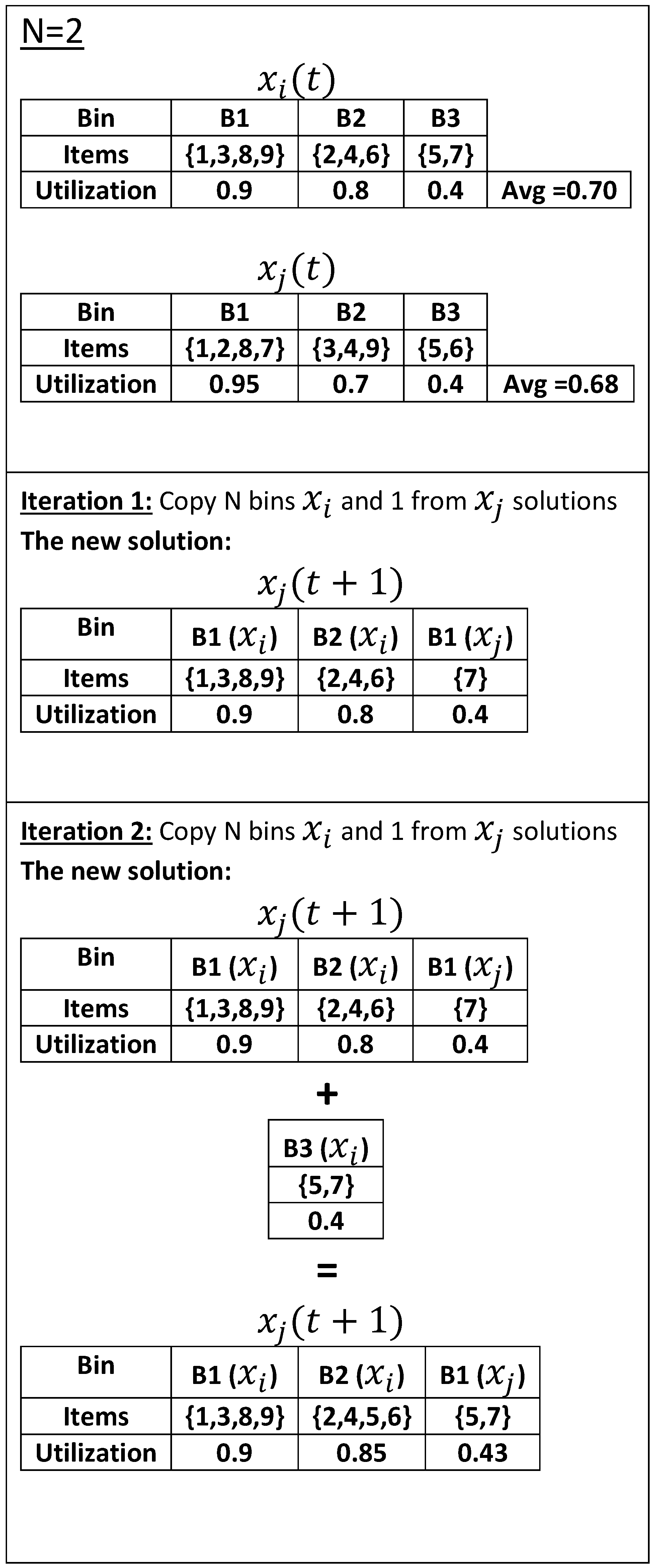
4.3. The Proposed Bin-Wise Level (AJS_B)

The intrinsic idea of the second proposed solution representation is to update the solution based on the evaluation of the bins. Thus, each bin’s utilization is computed before updating the solution, and bins satisfying certain criteria are selected as the sources of items to be swapped. Thus, the main difference between the two proposed solution representations is only the individual update step. In the following, we detail this step, while the other steps of the JS algorithm have been discussed in the previous subsection.
X i ( t + 1 ) = X i ( t ) r a n d ( 0 , B 1 ) ( σ ( X i ( t ) ) ) .
In Equation (28), the BPPCs solution, i.e., the JF, will be updated using three terms. First, X i ( t ) represents the current solution for the bin packing problem. Second, r a n d ( 0 , B 1 ) represents a random generator that selects one bin rather than the bin with the lowest utilization score, where B represents the number of bins in the solution. Third, the  σ function selects the bin with the lowest utilization score. The ⊡ operator moves the elements from the bin returned from σ ( X i ( t ) ) to the randomly selected bin in the second term of Equation (28). Equation (28) is repeated several times until the bin returned from σ ( X i ( t ) ) becomes empty. Thus, the BPPCs solution, i.e., the JF, is updated by removing the bin with the lowest utilization to another randomly selected bin(s).
X i ( t + 1 ) = X ( t ) i d i r e c t i o n
d i r e c t i o n = X j ( N 1 ) X i if f ( X i ) > = f ( X i ) X i ( N 1 ) X j if f ( X i ) < f ( X i ) .
In the second type of JS solution update, two JFs are used to update one of them. In the bin-wise representation, type B updating is accomplished. using Equation (30). In Equation (30), the ( N 1 ) symbol represents the update process, where the new updated solution is produced by merging the two solutions X i and X j as follows. Each solution sorts its bins by the utilization of the score. The average bin utilization of each solution is computed. Then, each solution contributes to the new solution by its share, where the solution with the better utilization contributes by N bins, and the other solution contributes by one bin. When the number of bins in a solution is greater than ( N + 1 ) , then Equation (30) is repeated until all the problem elements are packed in the bins.
In the following motivational example, the idea of bin-wise solution representation is explained. In Figure 7, a BPPCs solution is depicted for three bins B 1 , B 2 , and  B 3 , with their assigned items and the utilization score and type A solution update of a single solution. As  B 3 has the lowest utilization score, the items of B 3 are moved to the other two bins. Thus, this operation can help in reducing the number of bins and increase the utilization of the other bins.
In Figure 8, a JS-type B update operation for two BPPCs solutions is depicted for three bins, B 1 , B 2 , and  B 3 with their assigned items and the utilization score of the two solutions. In Figure 8, the given value is N = 2 . The new solution is created through two iterations. In each iteration, one bin is taken from the solution with the higher average utilization and one bin is taken from the other solution, where the duplicated items are discarded. In Figure 8, the  x i ( t ) has a higher average utilization score. In iteration 1 of Figure 8, B 1 and B 2 are copied from x i ( t ) , and B 1 is copied from x j ( t ) , where items 1, 2, and 8 are removed, as they appear in B 1 and B 2 from x i ( t ) . In the second iteration, B 3 is copied from x i ( t ) , and its items are assigned to the existing bins without duplication. Thus, item 5 is added to the last bin, as it is the only bin with empty space.
The overall steps of the proposed adaptive jellyfish search algorithm are listed in Algorithm 1 and can be summarized as follows. In lines 1 and 2, the initial parameters of the proposed algorithm are initialized, such as the number of jellyfishes in the population p s , the number of items to be packed into bins U b , the bin capacity C, the optimal number of bins m * , the number of bins in the reached solution m b e s t , the total number of iterations, and the initialization of the first iteration to 1 ( t = 1 ). Line 3 generates randomly valid initial packing solutions (i.e., the population) to the BPPCs instance, which guarantees the capacity constraint and the conflict constraint. Thus, the items are placed in random bins. Each solution in the population is evaluated according to the predefined objective function and assigned the best one to the global best individual X * according to lines 4 and 5, respectively. The motion of the jellyfish depends on the value of control parameter c ( t ) at each iteration, as listed in line 6. Based on that value (i.e., line 7), each jellyfish updates its position by following the ocean current at line 8 or by moving inside the swarm. Movement inside the swarm depends on a generated random value r a n d ( 0 , 1 ) compared to the c ( t ) (line 9) to be either passive or active. In line 10, the jellyfish moves to a new position according to type A (i.e., passive) based on its representation (i.e., either item-wise or bin-wise) while moving according to type B (i.e., active) in each representation at line 11. Once all the individuals in the population are updated (i.e., the new population), the fitness value of each jellyfish in the new population can be computed and updated to the global best one as in lines 12 and 13. In line 14, if the total number of used bins has reached the optimal number of bins; then, the algorithm stops searching and reports the optimal solution. Otherwise, the iteration number is incremented, and while it does not reach the predefined maximum number of iterations t m a x , steps 6 to 16 are repeated. In case of reaching the maximum number of iterations or the optimal number of bins, the global best solution is returned that represents the best packing of the items, as in line 17.
Algorithm 1 The proposed AJS algorithm.
Mathematics 11 03219 i001

5. Results and Discussion

5.1. Dataset

To evaluate the proposed methods, the benchmark dataset proposed in [20] was utilized. It is a publicly available dataset (http://or.dei.unibo.it/library/bin-packing-problem-conflicts, accessed on 1 June 2023). The dataset consists of 10 classes; the difference between the classes is the number of items. The higher the number of the class is, the more the number of items to be packed and the harder the problem is. Within a single class, there are 100 instances with a varied number of conflict items. The level of difficulty in each class has ten levels as well. The dataset has been used to evaluate several algorithms, such as [19,33].
They do not actually group these instances by edge densities δ but based on a threshold value d . The relation between δ and d is presented in [19] and described below in Table 2.
The values of d correspond to those derived using the formula of the edge density δ (i.e., δ = 2 | E | / n ( n 1 ) ) of the graph G based on d [20]. Specifically, according to the following equation, n represents the number of nodes in G.
δ = f ( d ) = 2 ( n d ) 2 n d n ( n 1 ) for d 0.5 n ( n 1 ) 2 n 2 ( 1 d ) 2 n ( 1 d ) n ( n 1 ) for d 0.5 .
Due to the computational complexity, only the first three classes of the dataset were utilized, where all ten levels of difficulty in each class were examined. In other words, the dataset in this work includes 27 different instances.

5.2. Setup

All experiments were implemented using Python 3.8 . The simulation experiments were performed on a computer running a 64-bit Linux OS with two 2.3 GHz Intel 8-core processors and 250 GB RAM.
In order to validate the proposed AJS algorithm for solving the BPPCs, a set of experiments were conducted over various instances from different classes of bin packing with the conflict dataset [52]. Table 3, Table 4 and Table 5 list the characteristics of some instances for three different classes, respectively. The number of items is N { 120 , 250 , 500 } , the bin capacity is C = 150 , the maximum degree for each instance is D, and the optimal number of bins is m * . The proposed algorithm aims to minimize the number of used bins and obtain bin utilization. The results of the proposed algorithm were compared against the most popular heuristics—First-Fit (FF) and Best-Fit (BF) [53]–and metaheuristics such as Particle Swarm Optimization (PSO) [54,55] and Jaya algorithm [56]. Table 6 lists all the algorithms’ setting parameters. Additionally, in order to achieve a fair comparison among the compared algorithms, all experiments were initiated with the same population size of 25 individuals (i.e., randomly packing solutions), and the maximum number of iterations ranged from 800 to 2000 iterations (i.e., t m a x = 800 for class 1, t m a x = 1500 for class 2, and t m a x = 2000 for class 3) as a stopping criteria, as well the optimal number of bins for each instance.
In the following subsections, the numerical results of each experiment and the performance analysis are discussed.

5.3. Evaluation Metrics

Each instance of the three classes was tested and evaluated to measure the quality of the proposed solution to the BPPCs. The minimum (min.), maximum (max.), average (avg.), and standard deviation (Std.) of the fitness values were computed over five independent runs. Moreover, the efficiency of the AJS against other compared algorithms on two metrics, namely, E f f and the improvement during iterations I P , can be computed by Equations (32) and (33), respectively.
E f f ( % ) = ( f A l g o f A J S ) / f A l g o ,
where A l g o = { F F , B F , P S O , J a y a } , f A l g o is the bins’ utilization of the compared algorithms, and f A J S is the bins’ utilization of the proposed adaptive jellyfish search algorithm.
I P = ( f i f j ) / f i ,
where f i and f j are the bins’ utilization of i t h and j t h run, respectively, and j is any consecutive run (i.e., j > i ).
According to the number of bins, the deviation D e v from the optimal number of each instance can be computed according to Equation (34) to measure the gap between the optimal solution and the global best solution.
D e v ( % ) = ( m b e s t m * ) / m b e s t ,
where m b e s t is the total number of used bins in the best solution, and m * is the optimal number of bins for each instance.

5.4. Results

The proposed adaptive jellyfish search algorithm AJS (i.e., both item-wise AJS_I and bin-wise AJS_B) and the heuristics (i.e., FF and BF) results from class 1 are shown in Table 7 and Table 8 in terms of the fitness values f v and number of bins, respectively.
Based on the fitness values from Table 7, the proposed algorithm, in the case of item-wise AJS_I and bin-wise AJS_B, achieved the smallest average minimum fitness values of 0.372 and 0.359, respectively, when compared with the FF value of 0.422 and the BF value of 0.411. For instance, using BPPC_1_3_3, as an example, the AJS_B and AJS_I obtained average fitness values of 0.080 and 0.095, respectively, while the f v of the FF heuristic equaled 0.223, and the BF heuristic equaled 0.198. Additionally, the efficiency of the AJS_I improved and reached up to 58 % when compared with the FF algorithm, and it reached up to 53 % when compared with the BF algorithm over various instances. In the case of the AJS_B, the eff reached up to 75 % and 72 % when compared with FF and BF, respectively, over various instances.
Table 8 lists all the instances’ packing solutions in terms of the number of used bins m b e s t relevant to the optimal number m * . Although the FF and BF are standard heuristics for solving a classical BPP, they failed to reach an optimal number of bins in the BPPCs for all test instances. However, both the proposed solutions (i.e., item-wise and bin-wise) reached a lower number of bins when compared with the heuristics. In addition, they reached the optimal number of test instances for some test instances (i.e., four test instances using AJS_B and 3 test instances using AJS_I.) For example, the AJS_I for solving BPPC_1_2_5 achieved the optimal packing of items (i.e., m * = m b e s t = 50 ), and both the AJS_I and AJS_B achieved the optimal packing for instance BPPC_1_9_4 (i.e., m * = m b e s t = 110 ). It is well noticed from the results that the first three instances achieved the best deviations in the case of the AJS_B when compared with the AJS_I, while, for the rest of the instances, the AJS_I had the smallest deviations from the optimal solution. Generally, the AJS_I and AJS_B achieved better average deviations of 0.018 % and 0.016 % , respectively, compared with the FF ( 0.053 % ) and BF ( 0.052 % ).
The proposed adaptive jellyfish search algorithm, AJS, has proven its efficiency in solving the BPPCs, not only when compared with the standard heuristics, but also when compared with other popular metaheuristics such as the PSO and Jaya, as shown in Table 9 and Table 10 in terms of the fitness function and the optimal number of bins, respectively.
From the results of Table 9, the proposed algorithm achieved the lowest average fitness value for all instances when compared with the Jaya and PSO. For example, the average of the AJS was equal to 0.197, while the averages of the Jaya and PSO were 0.229 and 0.589, respectively, for instance BPPC_1_4_2. Moreover, the AJS achieved the lowest average minimum fitness value, with instances equal to 0.360. The efficiency of the proposed algorithm improved and reached up to 84 % when compared with the Jaya and ranged from 3 % to 92 % when compared with the PSO.
Table 10 lists the m b e s t and D e v for the compared metaheuristics algorithms for all test instances. Although the Jaya algorithm reached the optimal number of bins in two instances (BPPC_1_7_2 and BPPC_1_9_4), the proposed AJS had a superior number of optimal bins for solving the BPPCs for five instances, with the smallest average deviation equaling 0.013 % over all instances. In contrast, the PSO had the poorest results, with larger average deviations of 0.226 % than the Jaya and AJS.
The main objective of the proposed work was to pack the conflict items into a minimum number of bins and achieve efficient bin utilization. For example, for solving instance BPPC_1_7_2, the AJS_I, AJS_B, and Jaya reached the optimal number of bins, but with different bins’ utilization. Figure 9 and Figure 10 show the convergence curve in terms of fitness value and the number of bins for solving that instance, respectively.
From Figure 9, the AJS_B achieved the smallest convergence curve during iterations, with an f v = 0.647 , and the I P reached up to 14 % . The PSO had the worst values for the iterations. Although the efficiency of the Jaya was better than the AJS_I within a range of 1 % 3 % , with more iterations, the AJS_I achieved a better efficiency with an f v = 0.655. In addition, the AJS_B had a superiority in reaching the optimal number of bins ( m b e s t = m * = 91 ) at a lower number of iterations ( t = 52 ) when compared with the others, as shown in Figure 10.
For more illustration in solving the BPP_1_2_5 instance, the proposed AJS was optimal in reaching both the minimum f v , as shown in Figure 11, and the m * , as shown in Figure 12.
At the beginning of the iterations (e.g., up to t = 50 ) at Figure 11, the proposed algorithm had a fast convergence in minimizing the fitness value when compared with the Jaya and PSO, with its e f f = 48 % better than the Jaya and its e f f = 79 % better than the PSO. With more iterations, the efficiency of AJS was up to 72 % better than the Jaya and up to 92 % better than the PSO. The performance of the AJS improved with increasing iterations ( I P ) within a range of 23∼42%.
In Figure 12, both the Jaya and PSO packed the items into 71 bins, while the AJS achieved a lower packing of items equaling 70 bins. Although the Jaya improved during iterations to minimize the number of used bins, it did not reach as optimal a number of bins by the end of iterations as the PSO. However, the AJS gained the optimality in the lowest number of iterations ( m b e s t = m * = 50 at t = 126 ).
For solving a BPPCs with a large number of items ( N = 250 , 500 ), as in Table 4 and Table 5), the proposed adaptive algorithm has proven its superiority in terms of achieving the lowest objective values compared with other heuristic and metaheuristic algorithms. Table 11 summarizes the average fitness values’ results for the class 2 and 3 instances.
For class 2, the AJS algorithm attained an average minimum f v over test instances equaling 0.343 , which was better than the average f v of the FF and BF by 15 % . Furthermore, when compared with the Jaya, the proposed algorithm had admirable results in average min., max., and average, where it reached up to 7 % and 46 % when compared with the PSO, respectively. Likewise, the average f v of the AJS algorithm equaled 0.326, while the FF, BF, Jaya, and PSO equaled 0.371, 0.370, 0.355, and 0.641, respectively, over the test instances of class 3. Regarding the average results, the AJS achieved improvement in minimizing the average fitness value by 8 % when compared with the Jaya and 49 % when compared with the PSO.
Regarding minimizing the number of used bins to the optimal packing for solving the class 2 and 3 instances, Table 12 lists the m b e s t and D e v results for all the algorithms. Although the proposed solution to the bin packing problem with conflicts did not reach the optimal number of bins for all instances (i.e., except for two test instances from class 2), it packed items into the smallest number of bins m b e s t compared with the standard heuristics and metaheuristics. For example, the AJS achieved the optimal packing of items m * = m b e s t = 102 for instance BPPC_2_2_3. However, the other compared algorithms reached a variant number of bins equal to 109, 110, 104, and 144 for the FF, BF, Jaya, and PSO, respectively.
From Table 12, the proposed adaptive jellyfish algorithm had an admirable lowest average deviation of overall test instances, which equaled 0.014. Its efficiency reached up to 70 % in comparison with the FF and 75 % when compared with the BF. Moreover, in comparison with the other metaheuristics, the AJS was better than the Jaya by 60 % and better than the PSO by 95 % .
For more details about the convergence curve of instance BPPC_2_2_2 as an example from class 2, Figure 13 and Figure 14 show the efficiency of the proposed solution for packing the items in terms of the objective function and number of bins during iterations.
Based on the two-fold aim of packing the items into a minimum number of bins with the best bins’ utilization, the AJS algorithm achieved a promising result. From Figure 13, the AJS had the smallest minimum f v of 0.019 , while the PSO and Jaya had an f v equal to 0.480 and 0.057 , respectively. The e f f of the proposed algorithm reached up to 96 % when compared with the PSO, while it improved within a range of 20 % 78 % when compared with the Jaya algorithm. During iterations, the solution was improved and reached the optimal number of bins m b e s t = m * = 100 at t = 841 , as shown in Figure 14. In contrast, these items were packed into 102 and 144 bins through the Jaya and PSO, respectively, at the end of the iterations.
Figure 15 shows the convergence curve of instance BPPC_3_3_9. The f v of the proposed algorithm decreased rapidly during the first iterations, with an I P reaching up to 88 % . Although the Jaya algorithm had a better minimization of the f v than the PSO until the end of the iterations, the AJS algorithm outperformed the compared algorithms with the smallest minimum of an f v = 0.013 . The Jaya algorithm reached an f v = 0.083 , and the PSO reached an f v = 0.541 . The e f f of the AJS ranged from 25 % to 98 % and from 18 % to 84 % in comparison with the PSO and Jaya, respectively.
Although all the compared algorithms did not reach the optimal number of bins for this instance (i.e., m * = 196 ), the AJS packed these items into the smallest number of bins (i.e., m b e s t = 197 ) compared with the others, as shown in Figure 16.
The proposed adaptive jellyfish search algorithm showed the best performance compared with other representative baseline algorithms according to the above results. It achieved the lowest average fitness value and the lowest number of used bins for solving BPPCs instances. To the best of our knowledge, this work is the first one that uses the jellyfish algorithm to solve the bin packing problem, especially when dealing with conflict items from the initial solution.

6. Conclusions

In this work, the bin packing problem with conflicts was addressed due to its impact on several applications. In addition, according to our knowledge, the literature includes very limited efforts in utilizing metaheuristic methods to address the BPPCs. In this vein, adapting the jellyfish algorithm to address the BBPCs using two solution representations was proposed. These two representations frame the BPPCs problem at two different levels: item-wise and bin-wise. The BPPCs solution representation can be framed as a sequence of item swaps, where the items to be swapped can be from any bin without any restrictions; this approach is called item-wise. On the other hand, some bins with certain conditions can be selected, and then the item swaps occur for this group of bins only; this approach is called bin-wise. Then, we proposed a set of operations that fit the BPPCs to be used as the jellyfish algorithm operations. These operations were used to update the solutions. Finally, the performance of the proposed methods was evaluated using a standard dataset with a known optimal number of bins. The evaluation included a set of methods of comparison, namely, the PSO, Jaya, and several heuristics. The comparison was performed to find solutions to two objectives: the number of bins and the average bin utilization. The obtained results showed that the proposed method’s performance was better than the other methods for the two objectives, and it yielded the smallest deviation rate from the optimal number of bins. The obtained results showed an improvement on the other methods of comparison by a range of least 2 to 18 times. However, the bin packing problem remains a big challenge, especially with conflicting items. As a result, some future research directions will be considered, such as a hybrid method to acquire more benefits, a test of the AJS against real-world scenarios, and and assessment of packing items in multidimensions or other multiobjective criteria.

Author Contributions

Conceptualization, W.H.E.-A., A.S. and A.F.; methodology, W.H.E.-A., M.B., G.X. and A.F.; software, W.H.E.-A., M.B., G.X. and A.F.; validation, W.H.E.-A. and M.B.; formal analysis, G.X. and K.A.R.; investigation, W.H.E.-A., A.S. and M.B.; resources, A.S. and G.X.; data curation, W.H.E.-A. and M.B.; writing—original draft preparation, W.H.E.-A. and M.B.; supervision, A.S., G.X., K.A.R. and A.F.; project administration, A.S. and A.F.; funding acquisition, K.A.R. All authors have read and agreed to the published version of the manuscript.

Funding

This research received no external funding.

Data Availability Statement

The utilized dataset of this work is publicly available: http://or.dei.unibo.it/library/bin-packing-problem-conflicts, accessed on 1 June 2023.

Conflicts of Interest

The authors have no relevant financial or nonfinancial interest to disclose.

References

  1. Tudosoiu, M.F.; Pop, F. Bin Packing Scheduling Algorithm with Energy Constraints in Cloud Computing. In Proceedings of the 2021 IEEE 17th International Conference on Intelligent Computer Communication and Processing (ICCP), Cluj-Napoca, Romania, 28–30 October 2021; pp. 77–84. [Google Scholar]
  2. Lin, Y.H.; Lin, C.; Lin, B. On conflict and cooperation in a two-echelon inventory model for deteriorating items. Comput. Ind. Eng. 2010, 59, 703–711. [Google Scholar] [CrossRef]
  3. Nguyen, T.H.; Nguyen, X.T. Space Splitting and Merging Technique for Online 3-D Bin Packing. Mathematics 2023, 11, 1912. [Google Scholar] [CrossRef]
  4. Moura, A.; Pinto, T.; Alves, C.; Valério de Carvalho, J. A Matheuristic Approach to the Integration of Three-Dimensional Bin Packing Problem and Vehicle Routing Problem with Simultaneous Delivery and Pickup. Mathematics 2023, 11, 713. [Google Scholar] [CrossRef]
  5. Labrada-Nueva, Y.; Cruz-Rosales, M.H.; Rendón-Mancha, J.M.; Rivera-López, R.; Eraña-Díaz, M.L.; Cruz-Chávez, M.A. Overlap detection in 2D amorphous shapes for paper optimization in digital printing presses. Mathematics 2021, 9, 1033. [Google Scholar] [CrossRef]
  6. Mandal, C.A.; Chakrabarti, P.P.; Ghose, S. Complexity of fragmentable object bin packing and an application. Comput. Math. Appl. 1998, 35, 91–97. [Google Scholar] [CrossRef] [Green Version]
  7. Shachnai, H.; Tamir, T.; Yehezkely, O. Approximation schemes for packing with item fragmentation. Theory Comput. Syst. 2008, 43, 81–98. [Google Scholar] [CrossRef] [Green Version]
  8. Byholm, B.; Porres, I. Fast algorithms for fragmentable items bin packing. J. Heuristics 2018, 24, 697–723. [Google Scholar] [CrossRef]
  9. Archetti, C.; Bianchessi, N.; Speranza, M.G. Branch-and-cut algorithms for the split delivery vehicle routing problem. Eur. J. Oper. Res. 2014, 238, 685–698. [Google Scholar] [CrossRef]
  10. Casazza, M.; Ceselli, A. Mathematical programming algorithms for bin packing problems with item fragmentation. Comput. Oper. Res. 2014, 46, 1–11. [Google Scholar] [CrossRef]
  11. Epstein, L.; Levin, A.; Van Stee, R. Approximation schemes for packing splittable items with cardinality constraints. Algorithmica 2012, 62, 102–129. [Google Scholar] [CrossRef]
  12. Casazza, M.; Ceselli, A. Exactly solving packing problems with fragmentation. Comput. Oper. Res. 2016, 75, 202–213. [Google Scholar] [CrossRef]
  13. Laporte, G.; Desroches, S. Examination timetabling by computer. Comput. Oper. Res. 1984, 11, 351–360. [Google Scholar] [CrossRef]
  14. Mingozzi, A. Loading Problems. In Combinatorial Optimization; 1979; p. 339. Available online: https://pubsonline.informs.org/doi/abs/10.1287/inte.11.5.113 (accessed on 29 May 2023).
  15. Jansen, K. An approximation scheme for bin packing with conflicts. J. Comb. Optim. 1999, 3, 363–377. [Google Scholar] [CrossRef]
  16. Sadykov, R.; Vanderbeck, F. Bin packing with conflicts: A generic branch-and-price algorithm. INFORMS J. Comput. 2013, 25, 244–255. [Google Scholar] [CrossRef] [Green Version]
  17. Minton, S.; Johnston, M.D.; Philips, A.B.; Laird, P. Minimizing conflicts: A heuristic repair method for constraint satisfaction and scheduling problems. Artif. Intell. 1992, 58, 161–205. [Google Scholar] [CrossRef] [Green Version]
  18. Balogh, J.; Békési, J.; Galambos, G. New lower bounds for certain classes of bin packing algorithms. Theor. Comput. Sci. 2012, 440, 1–13. [Google Scholar] [CrossRef] [Green Version]
  19. Muritiba, A.E.F.; Iori, M.; Malaguti, E.; Toth, P. Algorithms for the bin packing problem with conflicts. INFORMS J. Comput. 2010, 22, 401–415. [Google Scholar] [CrossRef]
  20. Gendreau, M.; Laporte, G.; Semet, F. Heuristics and lower bounds for the bin packing problem with conflicts. Comput. Oper. Res. 2004, 31, 347–358. [Google Scholar] [CrossRef]
  21. Elhedhli, S.; Li, L.; Gzara, M.; Naoum-Sawaya, J. A branch-and-price algorithm for the bin packing problem with conflicts. INFORMS J. Comput. 2011, 23, 404–415. [Google Scholar] [CrossRef]
  22. Khanafer, A.; Clautiaux, F.; Talbi, E.G. New lower bounds for bin packing problems with conflicts. Eur. J. Oper. Res. 2010, 206, 281–288. [Google Scholar] [CrossRef]
  23. Gogos, C.; Alefragis, P.; Housos, E. An improved multi-staged algorithmic process for the solution of the examination timetabling problem. Ann. Oper. Res. 2012, 194, 203–221. [Google Scholar] [CrossRef]
  24. Antal, M.; Pop, C.; Cioara, T.; Anghel, I.; Salomie, I.; Pop, F. A system of systems approach for data centers optimization and integration into smart energy grids. Future Gener. Comput. Syst. 2020, 105, 948–963. [Google Scholar] [CrossRef]
  25. Garey, M.R.; Johnson, D.S. Computers and Intractability; Freeman: San Francisco, CA, USA, 1979; Volume 174. [Google Scholar]
  26. Coffman, E.G., Jr.; Csirik, J.; Galambos, G.; Martello, S.; Vigo, D. Bin Packing Approximation Algorithms: Survey and Classification; Springer: New York, NY, USA, 2013; pp. 455–531. [Google Scholar]
  27. Delorme, M.; Iori, M.; Martello, S. Bin packing and cutting stock problems: Mathematical models and exact algorithms. Eur. J. Oper. Res. 2016, 255, 1–20. [Google Scholar] [CrossRef]
  28. Epstein, L.; Levin, A. On bin packing with conflicts. SIAM J. Optim. 2008, 19, 1270–1298. [Google Scholar] [CrossRef]
  29. Dósa, G.; Sgall, J. First Fit bin packing: A tight analysis. In Proceedings of the 30th International Symposium on Theoretical Aspects of Computer Science (STACS 2013), Kiel, Germany, 27 February–2 March 2013. [Google Scholar]
  30. Fathalla, A.; Li, K.; Salah, A. Best-KFF: A multi-objective preemptive resource allocation policy for cloud computing systems. Clust. Comput. 2022, 25, 321–336. [Google Scholar] [CrossRef]
  31. Martello, S.; Toth, P. Lower bounds and reduction procedures for the bin packing problem. Discret. Appl. Math. 1990, 28, 59–70. [Google Scholar] [CrossRef]
  32. Scholl, A.; Klein, R.; Jürgens, C. Bison: A fast hybrid procedure for exactly solving the one-dimensional bin packing problem. Comput. Oper. Res. 1997, 24, 627–645. [Google Scholar] [CrossRef]
  33. Brandao, F.; Pedroso, J.P. Bin packing and related problems: General arc-flow formulation with graph compression. Comput. Oper. Res. 2016, 69, 56–67. [Google Scholar] [CrossRef] [Green Version]
  34. De Carvalho, J.V. Exact solution of bin-packing problems using column generation and branch-and-bound. Ann. Oper. Res. 1999, 86, 629–659. [Google Scholar] [CrossRef]
  35. Bourjolly, J.M.; Rebetez, V. An analysis of lower bound procedures for the bin packing problem. Comput. Oper. Res. 2005, 32, 395–405. [Google Scholar] [CrossRef]
  36. Stawowy, A. Evolutionary based heuristic for bin packing problem. Comput. Ind. Eng. 2008, 55, 465–474. [Google Scholar] [CrossRef]
  37. Loh, K.H.; Golden, B.; Wasil, E. Solving the one-dimensional bin packing problem with a weight annealing heuristic. Comput. Oper. Res. 2008, 35, 2283–2291. [Google Scholar] [CrossRef]
  38. Kucukyilmaz, T.; Kiziloz, H.E. Cooperative parallel grouping genetic algorithm for the one-dimensional bin packing problem. Comput. Ind. Eng. 2018, 125, 157–170. [Google Scholar] [CrossRef]
  39. Galinier, P.; Hao, J.K. Hybrid evolutionary algorithms for graph coloring. J. Comb. Optim. 1999, 3, 379–397. [Google Scholar] [CrossRef] [Green Version]
  40. Morgenstern, C. Distributed coloration neighborhood search. Discret. Math. Theor. Comput. Sci. 1996, 26, 335–358. [Google Scholar]
  41. Falkenauer, E. A hybrid grouping genetic algorithm for bin packing. J. Heuristics 1996, 2, 5–30. [Google Scholar] [CrossRef] [Green Version]
  42. Fleszar, K.; Charalambous, C. Average-weight-controlled bin-oriented heuristics for the one-dimensional bin-packing problem. Eur. J. Oper. Res. 2011, 210, 176–184. [Google Scholar] [CrossRef]
  43. Quiroz-Castellanos, M.; Cruz-Reyes, L.; Torres-Jimenez, J.; Gómez, C.; Huacuja, H.J.F.; Alvim, A.C. A grouping genetic algorithm with controlled gene transmission for the bin packing problem. Comput. Oper. Res. 2015, 55, 52–64. [Google Scholar] [CrossRef]
  44. Chou, J.S.; Truong, D.N. A novel metaheuristic optimizer inspired by behavior of jellyfish in ocean. Appl. Math. Comput. 2021, 389, 125535. [Google Scholar] [CrossRef]
  45. Fossette, S.; Putman, N.F.; Lohmann, K.J.; Marsh, R.; Hays, G.C. A biologist’s guide to assessing ocean currents: A review. Mar. Ecol. Prog. Ser. 2012, 457, 285–301. [Google Scholar] [CrossRef] [Green Version]
  46. Fossette, S.; Gleiss, A.C.; Chalumeau, J.; Bastian, T.; Armstrong, C.D.; Vandenabeele, S.; Karpytchev, M.; Hays, G.C. Current-oriented swimming by jellyfish and its role in bloom maintenance. Curr. Biol. 2015, 25, 342–347. [Google Scholar] [CrossRef] [Green Version]
  47. Mariottini, G.L.; Pane, L. Mediterranean jellyfish venoms: A review on scyphomedusae. Mar. Drugs 2010, 8, 1122–1152. [Google Scholar] [CrossRef] [PubMed] [Green Version]
  48. Brotz, L.; Cheung, W.W.; Kleisner, K.; Pakhomov, E.; Pauly, D. Increasing jellyfish populations: Trends in large marine ecosystems. In Jellyfish Blooms IV; Springer: Berlin/Heidelberg, Germany, 2012; pp. 3–20. [Google Scholar]
  49. Dong, Z.; Liu, D.; Keesing, J.K. Jellyfish blooms in China: Dominant species, causes and consequences. Mar. Pollut. Bull. 2010, 60, 954–963. [Google Scholar] [CrossRef] [PubMed]
  50. Zavodnik, D. Spatial aggregations of the swarming jellyfish Pelagia noctiluca (Scyphozoa). Mar. Biol. 1987, 94, 265–269. [Google Scholar] [CrossRef]
  51. Kiran, M.S.; Hakli, H.; Gunduz, M.; Uguz, H. Artificial bee colony algorithm with variable search strategy for continuous optimization. Inf. Sci. 2015, 300, 140–157. [Google Scholar] [CrossRef]
  52. BPPC Dataset. Available online: http://or.dei.unibo.it/library/bin-packing-problem-conflicts (accessed on 5 September 2021).
  53. Johnson, D.S.; Demers, A.J.; Ullman, J.D.; Garey, M.R.; Graham, R.L. Worst-Case Performance Bounds for Simple One-Dimensional Packing Algorithms. SIAM J. Comput. 1974, 3, 299–325. [Google Scholar] [CrossRef] [Green Version]
  54. Kennedy, J.; Eberhart, R. Particle swarm optimization. In Proceedings of the ICNN’95—International Conference on Neural Networks, Perth, Australia, 27 November–1 December 1995; Volume 4, pp. 1942–1948. [Google Scholar] [CrossRef]
  55. Yan, J.; He, W.; Jiang, X.; Zhang, Z. A novel phase performance evaluation method for particle swarm optimization algorithms using velocity-based state estimation. Appl. Soft Comput. 2017, 57, 517–525. [Google Scholar] [CrossRef]
  56. Venkata Rao, R. Jaya: A simple and new optimization algorithm for solving constrained and unconstrained optimization problems. Int. J. Ind. Eng. Comput. 2016, 7, 19–34. [Google Scholar] [CrossRef]
Figure 1. A flowchart of the proposed method.
Mathematics 11 03219 g001
Figure 7. An example of type A solution update for the bin-wise representation.
Mathematics 11 03219 g007
Figure 8. An example of type B solution update for the bin-wise representation.
Mathematics 11 03219 g008
Figure 9. Convergence curve of instance BPPC_1_7_2.
Mathematics 11 03219 g009
Figure 10. Number of bins of instance BPPC_1_7_2.
Mathematics 11 03219 g010
Figure 11. Convergence curve of instance BPPC_1_2_5.
Mathematics 11 03219 g011
Figure 12. Number of bins of instance BPPC_1_2_5.
Mathematics 11 03219 g012
Figure 13. Convergence Curve of instance BPPC_2_2_2.
Mathematics 11 03219 g013
Figure 14. Number of bins of instance BPPC_2_2_2.
Mathematics 11 03219 g014
Figure 15. Convergence curve of instance BPPC_3_3_9.
Mathematics 11 03219 g015
Figure 16. Number of bins of instance BPPC_3_3_9.
Mathematics 11 03219 g016
Table 1. A comparison of research works addressing the BPP-based problems.
PaperBPPC MethodMethodologyObjectives and Results
 [36]Weight Annealing MethodologyUsing the WA concept, develops a straightforward procedure for the one-dimensional BPP.Covered the majority of relevant Hadoop constraints and achieved comparable performance with FIFO and Fair Schedulers.
 [37]Multi-Capacity Bin Packing Problems (MCBPP) and Machine Reassignment Problems (MRP)Multi-Start Iterated Local Search (MS-ILS-PPs)Maximized machine utilization and cost-efficient task reassignment, improved upper bounds and achieved near-optimal solutions.
 [38]The Island-Parallel Grouping Genetic Algorithm (IPGGA)Creates a parallelized version of an evolutionary algorithm for the 1DBPP. Evaluates different model parameters.Achieved optimal solutions for 23 of 28 instances of the Hard28 dataset, thus outperforming earlier models. Results showed that, for widely distributed computing, dynamic communication topologies are more suitable.
 [43]One-Dimensional Bin Packing Problem (BPP)Grouping Genetic Algorithm with Controlled Gene Transmission (GGA-CGT)The GGA-CGT was created to promote the transmission of the best genes of the chromosomes and to explore the search space while balancing selective pressure and population diversity to prevent premature convergence. With respect to the Hard28 set, the method outperformed state-of-the-art algorithms.
Table 2. Relationship between δ and d .
d 0 0.1 0.2 0.3 0.4 0.5 0.6 0.7 0.8 0.9
δ 0 0.2 0.8 0.18 0.32 0.5 0.68 0.82 0.92 0.98
Table 3. Class 1 ( N = 120 and C = 150 ).
Instance No.Maximum Degree (D)Optimal No. of Bins ( m * )
BPPC_1_1_11848
BPPC_1_2_54150
BPPC_1_3_37346
BPPC_1_4_29653
BPPC_1_5_511957
BPPC_1_6_311975
BPPC_1_7_211991
BPPC_1_8_611999
BPPC_1_9_4119110
Table 4. Class 2 ( N = 250 and C = 150 ).
Instance No.Maximum Degree (D)Optimal No. of Bins ( m * )
BPPC_2_1_340102
BPPC_2_2_299100
BPPC_2_3_5149101
BPPC_2_4_6199109
BPPC_2_5_7249126
BPPC_2_6_7249147
BPPC_2_7_5249181
BPPC_2_8_5249205
BPPC_2_9_2249225
Table 5. Class 3 ( N = 500 and C = 150 ).
Instance No.Maximum Degree (D)Optimal No. of Bins ( m * )
BPPC_3_1_3105202
BPPC_3_2_1207198
BPPC_3_3_9296196
BPPC_3_4_5393206
BPPC_3_5_8499241
BPPC_3_6_4499307
BPPC_3_7_5499343
BPPC_3_8_5499400
BPPC_3_9_2499444
Table 6. Algorithms’ parameters.
AlgorithmParametersDefinitionValue
PSO c 1 and c 2 The acceleration coefficients2
Jaya r 1 and r 2 Learning parameters [ 0 , 1 ]
AJS c ( t ) Switching parameter [ 0 , 1 ]
γ A motion coefficient [ U b , L b ]
Table 7. Class 1 fitness value (FF, BF, AJS_I and AJS_B).
Instance No.FFBFAJS_IAJS_B
f v f v Min.Max.Avg. ± Std.Min.Max.Avg. ± Std.
BPPC_1_1_10.1320.1070.0680.0710.070 ± 0.0010.0330.0330.033 ± 0.000
BPPC_1_2_50.1090.1090.0660.0720.069 ± 0.0030.0370.0380.038 ± 0.000
BPPC_1_3_30.2230.1980.0940.0970.095 ± 0.0010.0560.1040.080 ± 0.017
BPPC_1_4_20.2660.2670.1910.2070.197 ± 0.0060.1950.2200.210 ± 0.009
BPPC_1_5_50.2970.2680.2250.2500.239 ± 0.0110.2290.2500.236 ± 0.008
BPPC_1_6_30.5860.5830.5610.5720.568 ± 0.0040.5500.5890.567 ± 0.015
BPPC_1_7_20.6770.6650.6550.6640.661 ± 0.0040.6470.6500.649 ± 0.001
BPPC_1_8_60.7340.7300.7140.7180.716 ± 0.0020.7160.7220.719 ± 0.002
BPPC_1_9_40.7750.7760.7700.7720.771 ± 0.0010.7660.7700.769 ± 0.002
Average0.4220.4110.372 0.359
Table 8. Class 1 no. of bins (FF, BF, AJS_I and AJS_B).
Instance No.OptimalFFBFAJS_IAJS_B
m * m b e s t D e v m b e s t D e v m b e s t D e v m b e s t D e v
BPPC_1_1_148510.059500.040490.020480.000
BPPC_1_2_550520.038520.038510.020500.000
BPPC_1_3_346530.132520.115480.042470.021
BPPC_1_4_253580.086590.102550.036560.054
BPPC_1_5_557600.050600.050580.017590.034
BPPC_1_6_375790.051800.063770.026770.026
BPPC_1_7_291930.022930.022910.000910.000
BPPC_1_8_6991020.0291020.029990.0001000.010
BPPC_1_9_41101110.0091110.0091100.0001100.000
Average 0.053 0.052 0.018 0.016
Table 9. Class 1 fitness value (AJS, Jaya and PSO).
instance_id AJSJayaPSO
BPPC_1_1_1Min.0.0330.0620.432
Max.0.0330.0710.469
Avg. ± Std.0.033 ± 0.0000.066 ± 0.0010.455 ± 0.014
BPPC_1_2_5Min.0.0370.0650.474
Max.0.0380.0680.485
Avg. ± Std.0.038 ± 0.0000.066 ± 0.0170.480 ± 0.005
BPPC_1_3_3Min.0.0560.0980.522
Max.0.1040.1440.555
Avg. ± Std.0.080 ± 0.0170.121 ± 0.0110.543 ± 0.014
BPPC_1_4_2Min.0.1910.2100.578
Max.0.2070.2400.595
Avg. ± Std.0.197 ± 0.0060.229 ± 0.0140.589 ± 0.007
BPPC_1_5_5Min.0.2250.2470.583
Max.0.2500.2810.628
Avg. ± Std.0.239 ± 0.0040.270 ± 0.0030.610 ± 0.019
BPPC_1_6_3Min.0.5610.5660.726
Max.0.5720.5720.739
Avg. ± Std.0.568 ± 0.0040.569 ± 0.0000.734 ± 0.006
BPPC_1_7_2Min.0.6550.6610.749
Max.0.6640.6610.757
Avg. ± Std.0.661 ± 0.0040.661 ± 0.0020.753 ± 0.004
BPPC_1_8_6Min.0.7140.7160.785
Max.0.7180.7210.791
Avg. ± Std.0.716 ± 0.0020.719 ± 0.0010.787 ± 0.003
BPPC_1_9_4Min.0.7700.7700.795
Max.0.7720.7720.798
Avg. ± Std.0.771 ± 0.0010.771 ± 0.0040.797 ± 0.001
AverageMin.0.3600.3770.627
Table 10. Class 1 no. of bins (AJS, Jaya, and PSO).
Instance No.OptimalAJSJayaPSO
m * m b e s t D e v m b e s t D e v m b e s t D e v
BPPC_1_1_148480.000490.020650.262
BPPC_1_2_550500.000510.020710.296
BPPC_1_3_346480.042480.042700.343
BPPC_1_4_253550.036560.054790.329
BPPC_1_5_557580.017590.034820.305
BPPC_1_6_375770.026780.038960.219
BPPC_1_7_291910.000910.0001040.125
BPPC_1_8_299990.0001000.0101120.116
BPPC_1_9_41101100.0001100.0001150.043
Average 0.013 0.024 0.226
Table 11. Classes 2 and 3 fitness values (FF, BF, AJS, Jaya, and PSO).
AlgorithmAverageClass No.
Class 2Class 3
FF f v 0.4020.371
BF f v 0.4030.370
AJSMin.0.3430.326
Max.0.3500.331
Avg. ± Std.0.346 ± 0.0030.329 ± 0.002
JayaMin.0.3650.355
Max.0.3740.360
Avg. ± Std.0.371 ± 0.0030.358 ± 0.002
PSOMin.0.6360.641
Max.0.6510.653
Avg. ± Std.0.644 ± 0.0060.647 ± 0.005
Table 12. Classes 2 and 3 no. of bins (FF, BF, AJS, Jaya, and PSO).
Instance No.FFBFAJSJayaPSO
m b e s t D e v m b e s t D e v m b e s t D e v m b e s t D e v m b e s t D e v
BPPC_2_1_31090.0641100.0731020.0001040.0191440.292
BPPC_2_2_21080.0741080.0741000.0001020.0201440.306
BPPC_2_3_51100.0821090.0731020.0101050.0381520.336
BPPC_2_4_61170.0681180.0761110.0181160.0601700.359
BPPC_2_5_71320.0451360.0741290.0231320.0451810.304
BPPC_2_6_71560.0581580.0701520.0331550.0522000.265
BPPC_2_7_51860.0271880.0371820.0051850.0222190.174
BPPC_2_8_52090.0192100.0242070.0102080.0142340.124
BPPC_2_9_22280.0132290.0172260.0042260.0042420.070
BPPC_3_1_32120.0472110.0432030.0052090.0332960.318
BPPC_3_2_12110.0622100.0571990.0052050.0342980.336
BPPC_3_3_92090.0622090.0621970.0052050.0443070.362
BPPC_3_4_52260.0882310.1082160.0462230.0763360.387
BPPC_3_5_82530.0472600.0732510.0402590.0693640.338
BPPC_3_6_43120.0163180.0353100.0103160.0284050.242
BPPC_3_7_53600.0473640.0583510.0233550.0344360.213
BPPC_3_8_34100.0244120.0294050.0124100.0244680.145
BPPC_3_9_54480.0094510.0164460.0044490.0114840.083
Average 0.047 0.055 0.014 0.035 0.258
Disclaimer/Publisher’s Note: The statements, opinions and data contained in all publications are solely those of the individual author(s) and contributor(s) and not of MDPI and/or the editor(s). MDPI and/or the editor(s) disclaim responsibility for any injury to people or property resulting from any ideas, methods, instructions or products referred to in the content.

