Article

GERPM: A Geographically Weighted Stacking Ensemble Learning-Based Urban Residential Rents Prediction Model

1
School of Statistics and Information, Shanghai University of International Business and Economics, Shanghai 201620, China
2
School of Computer Science, Fudan University, Shanghai 200438, China
3
Shanghai Key Laboratory of Data Science, Shanghai 200438, China
*
Author to whom correspondence should be addressed.
Mathematics 2023, 11(14), 3160; https://doi.org/10.3390/math11143160
Submission received: 30 May 2023 / Revised: 1 July 2023 / Accepted: 7 July 2023 / Published: 18 July 2023
(This article belongs to the Special Issue Advances in Machine Learning and Applications)

Abstract

:
Accurate prediction of urban residential rents is of great importance for landlords, tenants, and investors. However, existing rents prediction models face challenges in meeting practical demands due to their limited perspectives and inadequate prediction performance. The existing individual prediction models often lack satisfactory accuracy, while ensemble learning models that combine multiple individual models to improve prediction results often overlook the impact of spatial heterogeneity on residential rents. To address these issues, this paper proposes a novel prediction model called GERPM, which stands for Geographically Weighted Stacking Ensemble Learning-Based Urban Residential Rents Prediction Model. GERPM comprehensively analyzes the influencing factors of residential rents from multiple perspectives and leverages a geographically weighted stacking ensemble learning approach. The model combines multiple machine learning and deep learning models, optimizes parameters to achieve optimal predictions, and incorporates the geographically weighted regression (GWR) model to consider spatial heterogeneity. By combining the strengths of deep learning and machine learning models and taking into account geographical factors, GERPM aims to improve prediction accuracy and provide robust predictions for urban residential rents. The model is evaluated using housing data from Nanjing, a major city in China, and compared with representative individual prediction models, the equal weight combination model, and the ensemble learning model. The experimental results demonstrate that GERPM outperforms other models in terms of prediction performance. Furthermore, the model’s effectiveness and robustness are validated by applying it to other major cities in China, such as Shanghai and Hangzhou. Overall, GERPM shows promising potential in accurately predicting urban residential rents and contributing to the advancement of the rental market.

1. Introduction

With the rapid development of society and increasing urbanization, cities are facing the challenge of accommodating a growing population. Given the high urban housing prices, renting has become an effective solution to address the accommodation problem. Accurate prediction of residential rents is essential for landlords, tenants, and investors alike. However, the housing rental market still faces challenges, such as information asymmetry. To overcome these barriers, it is necessary to conduct a comprehensive analysis of the factors influencing residential rents and develop accurate prediction models. This can benefit landlords in setting reasonable prices, assist investors in making informed decisions, enable tenants to understand the rental market and choose suitable options, and promote the healthy development of the housing rental market.
Previous research in the field of rental price prediction has mainly focused on traditional hedonic price models, time series models, and machine learning techniques. While advancements have been made by incorporating deep learning models and ensemble learning methods, there are still gaps and opportunities for further improvement.
Firstly, existing rental price prediction models often suffer from relatively low accuracy. Most of these models are individual predictors, and their performance is inadequate when the dataset contains noise [1]. Although some models [2,3] have improved prediction accuracy by combining multiple individual models through ensemble learning, they do not consider the spatial heterogeneity of residential rents or the significance of geographical factors on housing rental prices. Previous studies [4,5,6] have indicated that rental housing demand is sensitive to geographical factors. Therefore, there is a need to explore complex spatial modeling techniques to better capture the heterogeneity and spatial patterns of rental prices.
Secondly, existing models often only consider the intrinsic attributes of rental properties as influencing factors, neglecting a comprehensive analysis of factors from multiple perspectives. It is necessary to thoroughly analyze the factors influencing rental prices and investigate the impact of other factors, such as environmental characteristics, regional characteristics, and economic development. Incorporating these factors into the prediction model can potentially yield more accurate and comprehensive results.
The primary goal of this research is to create a precise rental price prediction model that incorporates spatial factors, various influencing factors, and advanced machine learning techniques. The gap analysis highlights the need for further research in complex spatial modeling techniques, exploration of additional influencing factors, and the application of advanced machine learning, deep learning, and ensemble learning methods. By addressing these gaps, this study aims to contribute to the existing literature and provide more accurate rental price predictions.
In this paper, we conduct a comprehensive analysis of the factors influencing rental prices from various perspectives, and propose a novel geographically weighted stacking ensemble learning-based urban residential rents prediction model, named GERPM. GERPM fully considers the spatial heterogeneity and conducts local regression prediction for different locations. Compared with the existing models, GERPM fully considers the spatial distribution characteristics of housing data and the impact of geographical location on rental prices. It incorporates several machine learning and deep learning models, including random forest, XGboost, LightGBM and CNN, which have shown good prediction performance, optimizes the parameters to achieve optimal prediction, and constructs a stacking ensemble learning model integrating Geographically weighted regression (GWR). The above machine learning and deep learning models serve as the base learners, and GWR serves as the meta learner. This approach leverages the predictive abilities of machine learning and deep learning while considering the influence of geographical factors on rental prices.
The proposed model is compared with other common predictive models to assess its prediction performance. Its effectiveness and robustness are verified using data from multiple cities. Additionally, the study acknowledges that factors influencing rental prices extend beyond the basic attributes of homes and encompass location characteristics, surrounding environmental facilities, and economic development, etc. Therefore, this research comprehensively considers the influencing factors, including home attributes, regional economic development, surrounding environment facilities, etc. [7,8,9]. Housing-related data are obtained through various sources and statistically analyzed. The influencing factors, such as the economic development of the area to which the home belongs, the medical facilities near the community, and the traffic situation, are quantitatively processed. The recursive feature elimination and random forest method are used to select influential variables that significantly impact rental prices. The main contributions of this paper are as follows:
  • Comprehensive analysis of factors influencing rental prices: Using Nanjing City in China as an example, this paper obtains housing-related data from various sources and conducts statistical analysis. This includes real data on rental prices and home attributes, point of interest (POI) data near homes provided by the Baidu Map Open Platform, and economic and demographic data of different regions from the website of the Bureau of Statistics. The study comprehensively analyzes the impact of architectural characteristics, environmental characteristics, and regional characteristics on rental prices and employs the recursive feature elimination and random forest method to select the feature variables that significantly influence rental prices for constructing a prediction model.
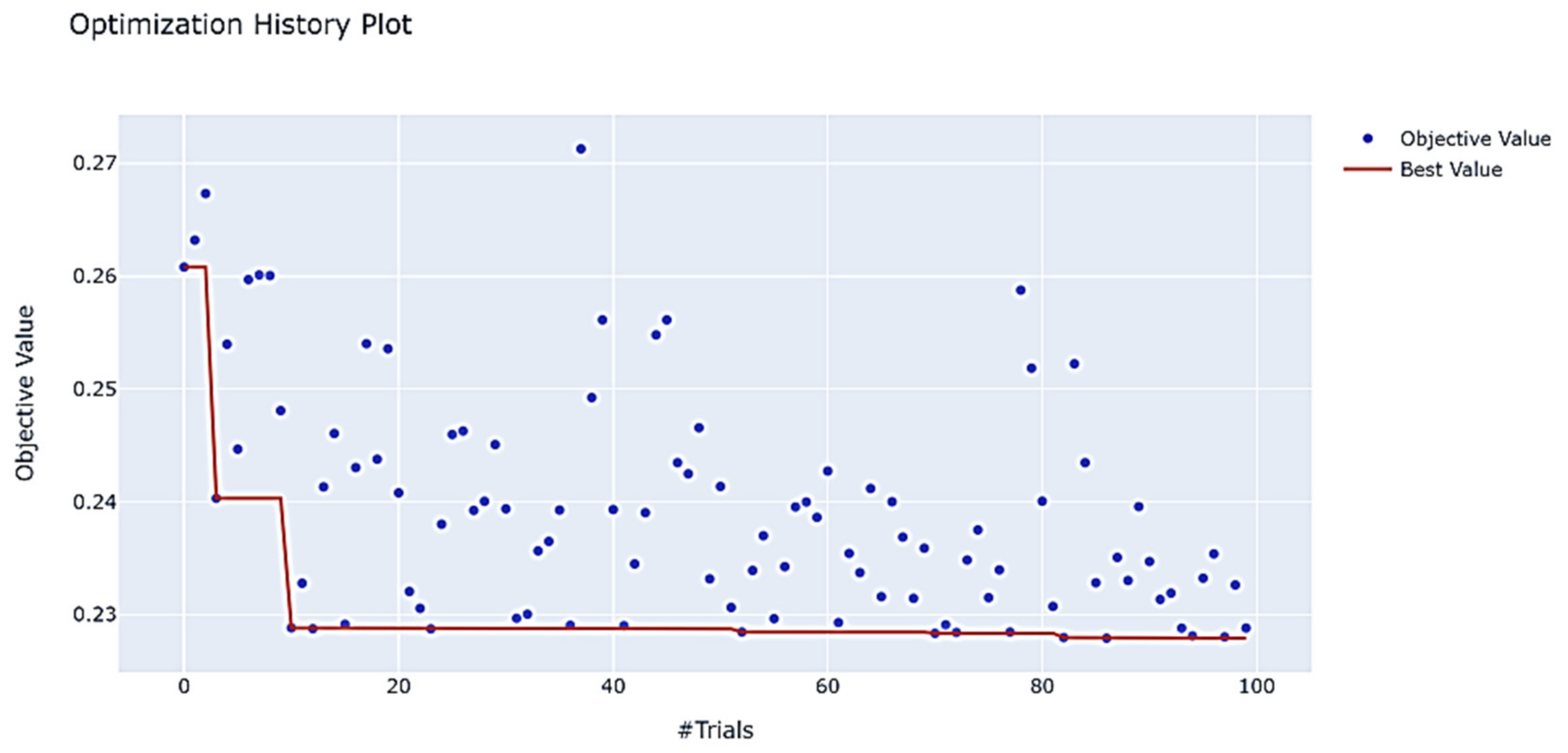
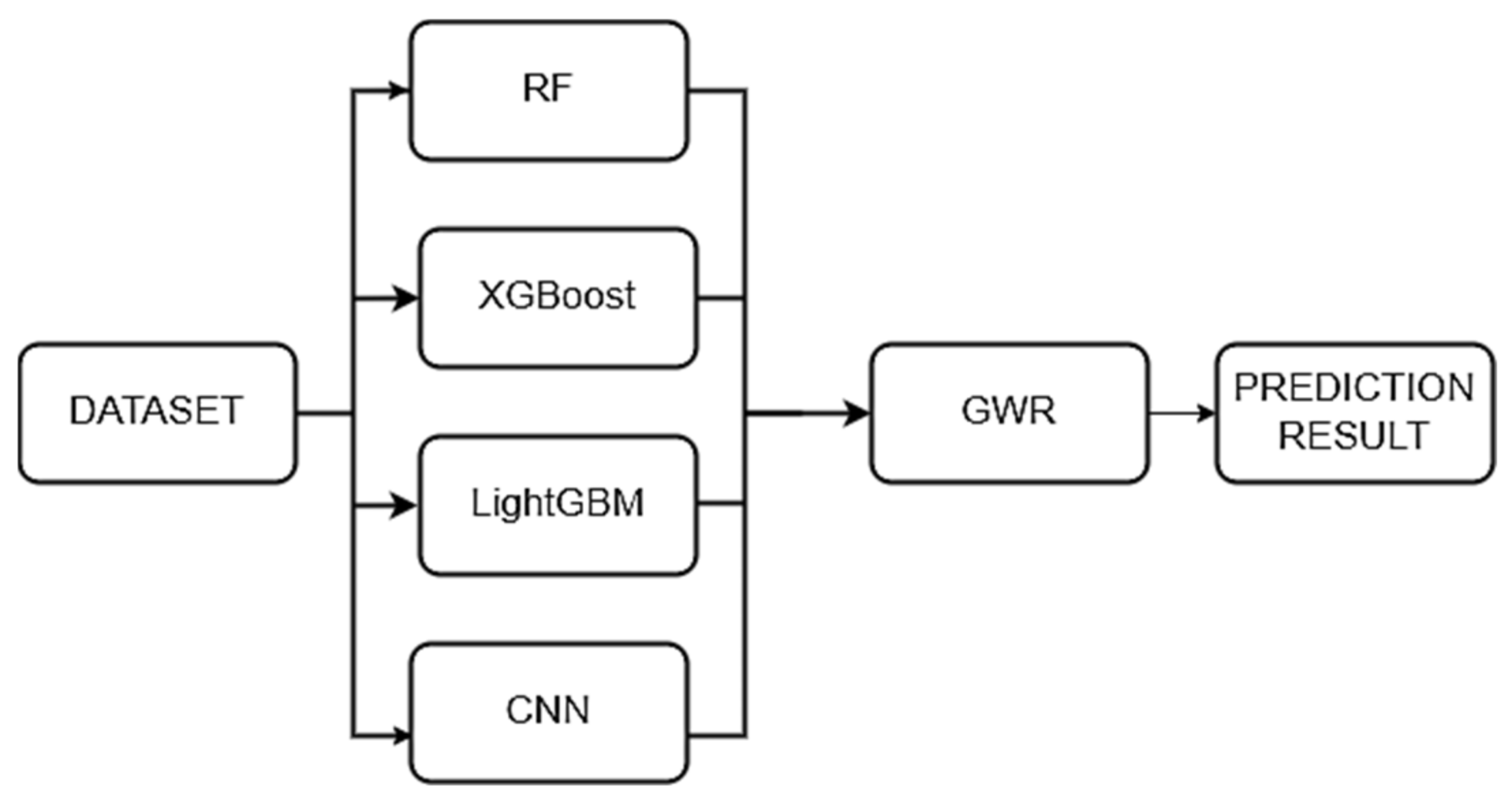
  • Development of the GERPM model: GERPM integrates random forest, XGBoost, LightGBM, and CNN models for rental price prediction. The Optuna framework is used for grid search and automatic parameter adjustment to optimize machine learning parameters. The parameter adjustment process is visualized to achieve optimal prediction results. Considering the influence of geographical location on rental prices, spatial autocorrelation testing is conducted, and a stacking-based ensemble learning model that integrates GWR is established. The aforementioned machine learning and deep learning models serve as base learners, while GWR serves as the meta learner.
  • Prediction results and robustness analysis: The prediction results of GERPM are compared with individual models, the equal weight combination model, and ensemble learning models that do not consider geographical factors. The performance of GERPM is evaluated using metrics such as mean square error (MSE), root mean square error (RMSE), and coefficient of determination (R2). In addition, GERPM is validated using housing data from other cities such as Shanghai and Hangzhou to assess its robustness.
The results demonstrate a significant clustering effect of rental prices in spatial distribution. In comparison to alternative prediction models, such as individual models, equal-weight combination models, and ensemble learning models that overlook geographical factors, GERPM exhibits remarkable prediction accuracy. The model consistently demonstrates outstanding performance across diverse datasets from various cities, affirming its robustness. Overall, GERPM exhibits promising potential in accurately forecasting urban residential rents and making contributions to the advancement of the rental market. In future studies, it is suggested to further explore the semantic heterogeneity and similarity between model parameters to enhance the performance of the model. In addition, the regional divisions can be refined in more detail. Also, the coverage of the dataset can be expanded to further enhance the model’s generalizability and adaptability.
The remainder of the paper is organized as follows: Section 2 provides an overview of relevant literature, Section 3 presents the methodology and details of the developed model, Section 4 presents the experimental results and analysis, and Section 5 concludes the paper.

2. Related Work

In terms of rental prices prediction, first of all, the hedonic price model is a commonly used rental prices prediction model in the early days. Valente et al. [10], based on the hedonic price model, added spatial variables, compared the rent changes in different regions, and used the new model to predict apartment rents to obtain more accurate results. Choi et al. [11] built a hedonic price model based on US housing data and found that energy-related utility costs, such as utility bills, are important factors affecting prices. In addition, spatial factors have also been considered in some studies. Han et al. [12] took the Salt Lake area as the research object, using the linear regression model, spatial lag model and geographically weighted regression model to explore the problem of heterogeneity, and found that the spatial heterogeneity in the eastern Salt Lake area was obvious, and the forest cover had a positive impact on residential value. Song et al. [13] analyzed the spatial differentiation and evolution based on Nanjing City’s 30-quarter housing price data, and found that the spatial differentiation of selling prices increased significantly. Through stepwise multiple regression analysis, it was found that geographical location had the highest degree of explanation for rental prices. In addition, models such as time series have also been applied. Liu et al. [14] established the gray prediction GM (1,1) model, VAR model and ARIMA model based on China’s Beijing city’s housing prices data, and found that only the prediction residual of the ARIMA model was uniformly distributed around 0, and its prediction effect was the best.
In recent years, machine learning [15,16,17,18,19,20,21] and deep learning [22,23,24,25] have been widely used for residential rents prediction for their good performance. Aziz et al. [22] studied the factors considered by Indonesian students in choosing boarding house rent, and used deep learning models to predict rent, which provided a reference for students to rent. Based on Airbnb rental data, Islam et al. [15] applied the XGBoost model based on Moran eigenvector spatial filtering to solve the spatial correlation problem and improve the prediction accuracy. Xie et al. [16] used machine learning models to predict the monthly rent of housing, and found that XGboost and LightGBM models were better than traditional GBDT models, and the influencing factors mainly included housing area and the location of the business district where the community was located. Liang et al. [17] selected rental housing data from China’s Shenzhen City, established random forest (RF), support vector machine (SVM), and XGBoost models for prediction, and used the grid search method to adjust the parameters and found that XGBoost had the best prediction effect. Liu et al. [18] selected rental housing data from four cities to discuss the impact of architectural characteristics, location characteristics, and environmental characteristics on housing rents. The researchers used multiple machine learning models to predict and found the random forest prediction effect was the best.
In the research of stacking ensemble learning, researchers have used various machine learning and deep learning models as learners to build stacking ensemble learning models, which have been widely applied in various fields and have achieved good predictive effects. In order to implement the short-term load prediction, based on the Spanish energy consumption data, Divina et al. [26] developed a stacking ensemble learning model with the evolutionary algorithms for regression trees, ANN and RF as base learners and GBM as the meta learner, which greatly improved the prediction accuracy. In order to predict the direction of the stock indexes, Jiang et al. [27] built a stacking ensemble learning model using machine learning models such as RF and XGBoost, and deep learning models such as RNN, GRU and LSTM as the first layer learners, whose output results were input into the Logistic model. The prediction results achieved high accuracy, F values, and AUC values. Kshatri et al. [28] implemented stacking ensemble learning with SVM and decision tree models based on crime data from India, providing an effective reference for crime-type prediction research.
Stacking ensemble learning [3,29,30,31] is also applied to home price prediction to improve the overall prediction accuracy. Lei et al. [29] took the hardbound properties in the Ames area as the research object, first established a number of single regression models to predict housing prices, and then used the prediction results of these single models as features to establish a multiple linear regression model, which improved the prediction accuracy. Zhang et al. [3] established several regression prediction models and machine learning models to predict the rental price, and constructed a stacking ensemble learning model with multiple linear regression as the meta learner. The results show that ensemble learning has the best prediction effect compared with the single based learner models and the weighted regression model. Truong et al. [30] established random forest, XGboost, and LightGBM models based on Beijing’s housing price data with a total of 26 variables. They combined the above models using the methods of hybrid regression and stacking ensemble learning respectively, and found that the hybrid regression has good generalization performance with a low time complexity, and its prediction accuracy is higher than that of the three single models. In addition, stacking ensemble learning had the best prediction performance with a high complexity.

3. Proposed Method

3.1. Preprocessing

3.1.1. Data

This paper initially selects China’s Nanjing City as the research subject to acquire related data through multiple channels. These sources include real rental prices and home attributes, POI data near homes offered by the Baidu Map Open Platform, and economic and demographic data of various regions supplied by the Bureau of Statistics website.
A total of 23,462 valid data samples are obtained. The relevant attributes of the rental homes are shown in Table 1.
By utilizing the location search service of the Baidu Maps open platform, we obtain POI data about the homes, including the nearest subway station distance, nearest bus station distance, nearest shopping mall distance, nearest hospital distance, number of supermarkets within 1000 m, number of office buildings within 1000 m, number of pharmacies within 1000 m, and number of parks within 1000 m.
Furthermore, the economic development level and population situation of the area where the home is located also significantly impact rental prices. Based on the 2021 main indicators of economic and social development in Nanjing provided on the website of the Nanjing Municipal Bureau of Statistics, the following indicators are selected as the influencing factors for predicting the rental price of the house in this study.
A—Population: The number of permanent residents across various regions of Nanjing.
B—Gross Domestic Product (GDP) of the district: The sum of the added value of various industries and the final outcome of production activities in the district.
C—General public budget revenue: Indicates the revenue and expenditure budget utilized to enhance people’s livelihoods and foster economic and social development.
D—Value added of the tertiary industry: Signifies the level of development of the economy.
E—Total retail sales of consumer goods: Reflects the material and cultural living standards of the people.
The above variables measure the differences in economic and social development levels among different districts of Nanjing from multiple perspectives. The summary of relevant data for each district is shown in Table 2.

3.1.2. Missing Value Processing

There are some uncontrollable factors in the process of data acquisition, which may lead to missing data. The primary approaches for handling missing data are as follows:
  • Delete: If a feature has more missing values and provides less information, it can be directly deleted. If there are fewer missing values for a feature, we can choose to delete the sample containing the missing value. This is a simple and direct method that is suitable for data with a large sample size and many features. However, when the proportion of missing value data is large, opting to directly delete the sample can disrupt the relationship between the data and affect the comprehensiveness of the data.
  • Imputation: If there are fewer missing values for a feature, directly deleting the feature may result in the loss of important information and affect the learning ability of the model. In this case, we can choose to fill in the data using the following methods: mean value filling, proximity value filling, maximum likelihood estimation filling, etc.
  • Non processing: Data deletion and imputation can alter the original dataset to a certain extent. Improper processing can introduce new noise and affect the accuracy of prediction. Using no processing methods can ensure the preservation of complete information from the original dataset.
In this paper, we summarize the missing values of variables in the obtained data by organizing the data, as shown in Table 3. Due to the large amount of total data, the missing values of the above variables account for a small proportion. In order to ensure the authenticity and validity of the data, 64 samples with missing values were deleted and 23,398 valid sample points were retained.

3.1.3. Handling of Abnormal Values

Outliers refer to data points that exhibit significant deviations from other observed values. Ignoring outliers can impact the prediction performance; hence, it is essential to test and address these values. Common methods for detecting abnormal values are as follows:
  • Statistical analysis: Conduct descriptive statistics on the dataset to obtain information such as mean, maximum, and minimum values. For example, we can use the describe function of the Pandas library in Python, and combine data visualization techniques such as scatter plots, histograms, and kernel density plots to observe the data distribution and identify outliers.
  • 3σ Principle: If the data follow a normal distribution or is close to a normal distribution, values that deviate from the average value by more than three times the standard deviation are considered abnormal values. Under this setting, the probability of data other than three times the standard deviation occurring is extremely small, and when it occurs, it can be considered an outlier.
  • Boxplot analysis: We can define Q 3 as the upper quartile and Q 1 as the lower quartile. Data points that are less than Q 1 1.5 Q 3 Q 1 or greater than Q 3 + 1.5 Q 3 Q 1 are considered outliers.
In this study, we first use the describe function in Python to conduct statistical descriptions, and find that there were significant outliers in price and area. We use Python’s matplotlib library to draw a price area scatter diagram for observation, as shown in Figure 1.
It can be observed that there is a positive correlation between area and price as a whole, and the price increases as the area increases. However, there are still some outliers, such as those with a large area but low price. Upon further investigation, it was discovered that the dataset contained some data points related to commercial office buildings and factory buildings. Since this study primarily focuses on residential properties, it is considered important to treat the above as outliers and delete them. These outliers are considered irrelevant and are subsequently removed. The 3 σ principle is then employed to filter out the abnormal values of the price, as illustrated in Figure 2. The red dots represent the outliers, and a total of 434 abnormal points are deleted. Ultimately, 22,964 valid points are retained.

3.1.4. Quantification of Categorical Features

One-Hot Encoding

For categorical variables, they cannot be directly incorporated into the model for computation and require encoding. The method used in this study is one-hot encoding. We employ the get_dummies function in Python to process the following six variables: gas, whether the whole lease, elevator, decoration, orientation, and floor. Among these, gas, whole lease status, elevator, and decoration each consist of two categories. The orientation variable contains multiple categories, with south-facing being the most significant factor affecting residential experience. Therefore, it is divided into two categories based on whether the property faces south. The floor variable comprises three categories: low floor, medium floor, and high floor. Some housing sources provide the floor number of the apartment and the total number of floors of the building. The following classification is performed: if the ratio of the floor number to the total number of floors is less than 0.33, it is classified as a low floor. If the ratio is between 0.33 and 0.66 (inclusive), it is classified as a middle floor. If the ratio is greater than 0.66, it is classified as a high floor. Taking the floor as an example, the comparison of results before and after one-hot encoding is shown in Table 4.

Quantification of Unit Type Variable

The unit type contains information about bedrooms, living rooms, and bathrooms, and the combination of quantities results in a large number of variable categories for the unit type, making it difficult to extract information. Therefore, the unit type variable is converted into three numerical variables based on the number of living rooms, bedrooms, and bathrooms.

3.1.5. Normalization of Numerical Features

The acquisition of variables encompasses numerous aspects, such as housing characteristics, the number of nearby infrastructure facilities, and distance. Different variables have significant differences in units and dimensions, which can introduce errors in subsequent modeling. Data normalization can eliminate the influence of dimensions, and there are two common normalization methods.

Min–Max Normalization

Min–max normalization employs a linear transformation technique to normalize data and map values into the [0, 1] interval, as illustrated in Equation (1). Here, x i is the original data, and x m a x and x m i n   are the maximum and minimum values, respectively.
x i = x i x min x max x min

Z-Score Normalization

Z-score normalization converts the original data into a dataset with a mean of 0 and a variance of 1, as shown in Equation (2), where   μ and σ are the mean and standard deviation of the original data.
z = X μ σ
Due to the considerable range of variable values, this study opts for Z-score normalization to process numerical independent variables, with the aim of mitigating the impact of excessive maximum and minimum values.

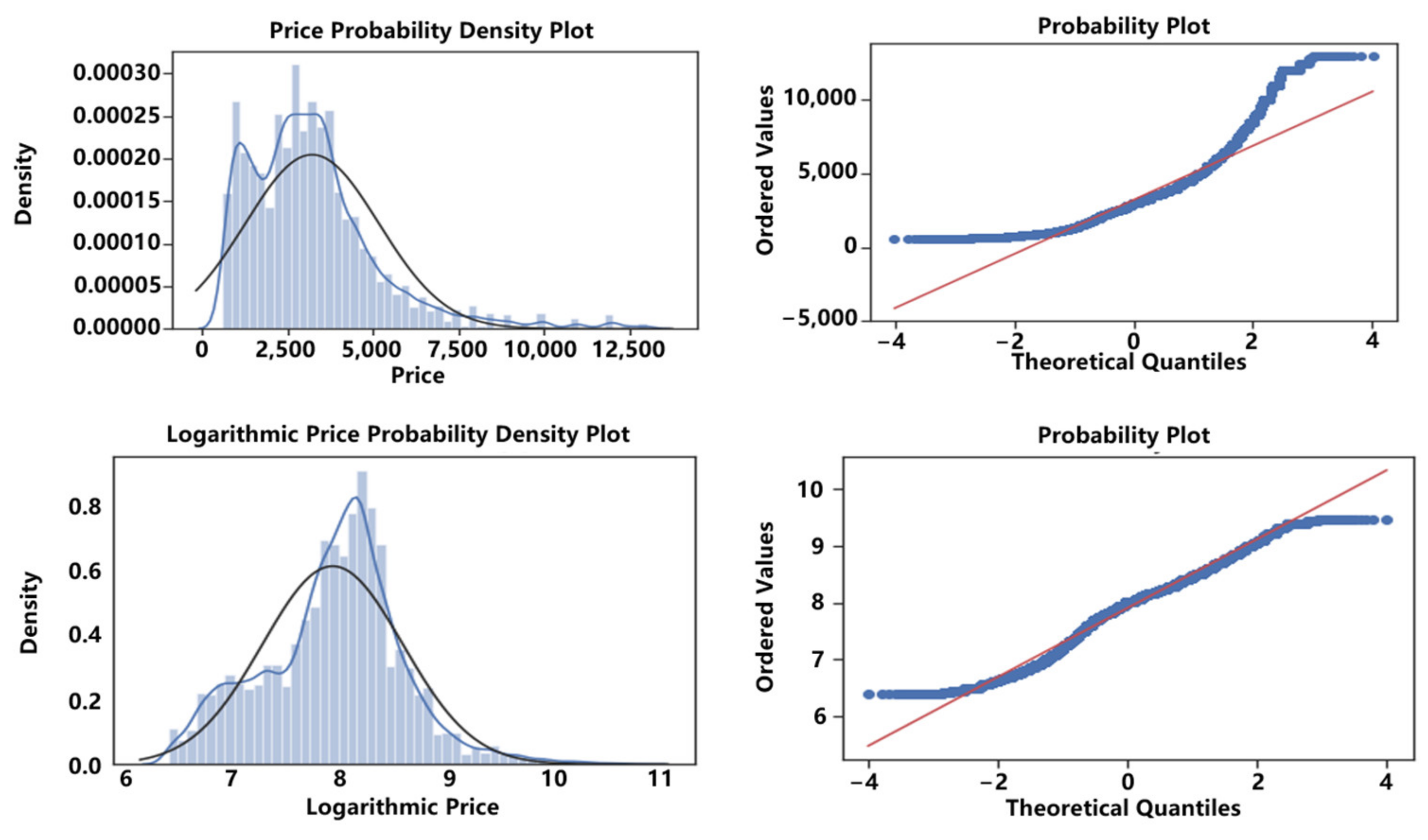
3.1.6. Logarithmic Processing of Dependent Variables

Upon conducting a statistical analysis of price variables, it is observed that they display a right-skewed distribution. Logarithmic processing is required to reduce the absolute differences between data points, resulting in a more uniform distribution of the price variable data. This approach helps mitigate the impact of extreme values and diminish prediction errors. The skewness coefficient and kurtosis coefficient are computed to represent the changes in distribution skewness following the logarithmization process. As demonstrated in Table 5, the skewness coefficient and kurtosis coefficient are significantly closer to zero, indicating that the right-skewness of the data has been effectively improved.

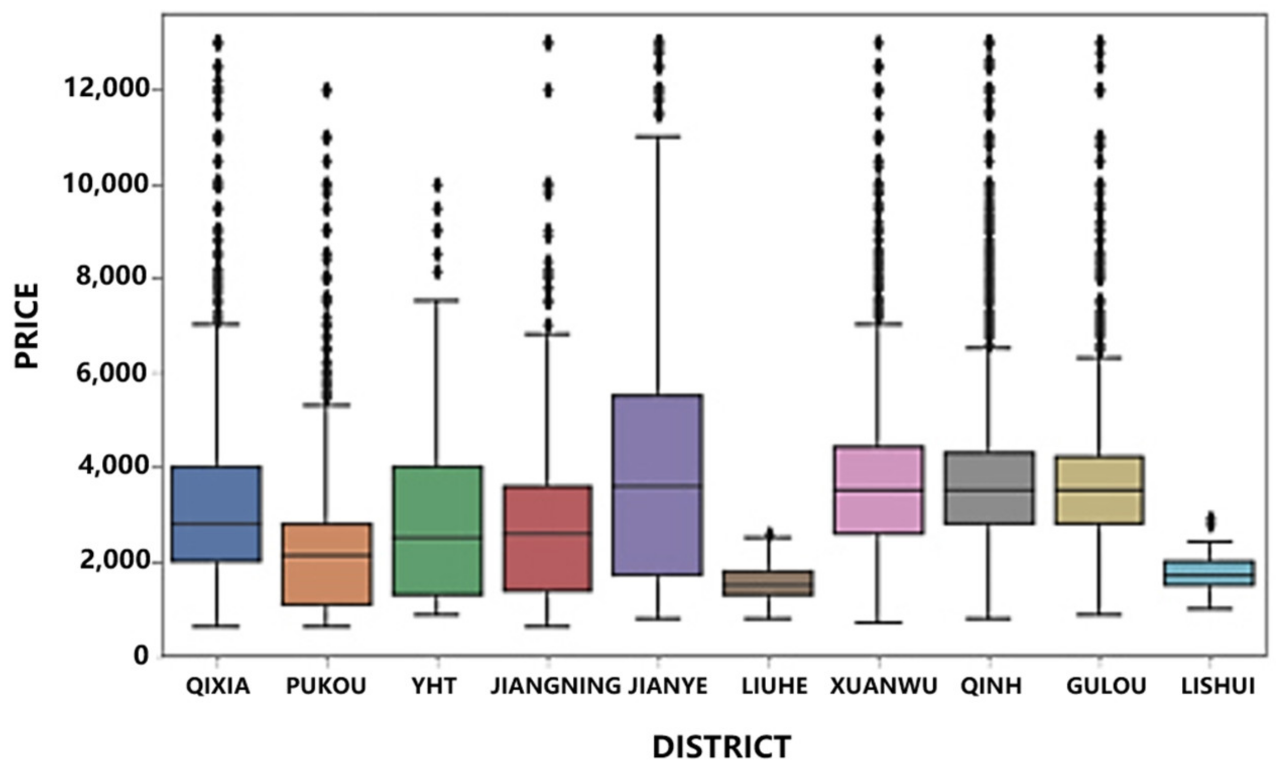
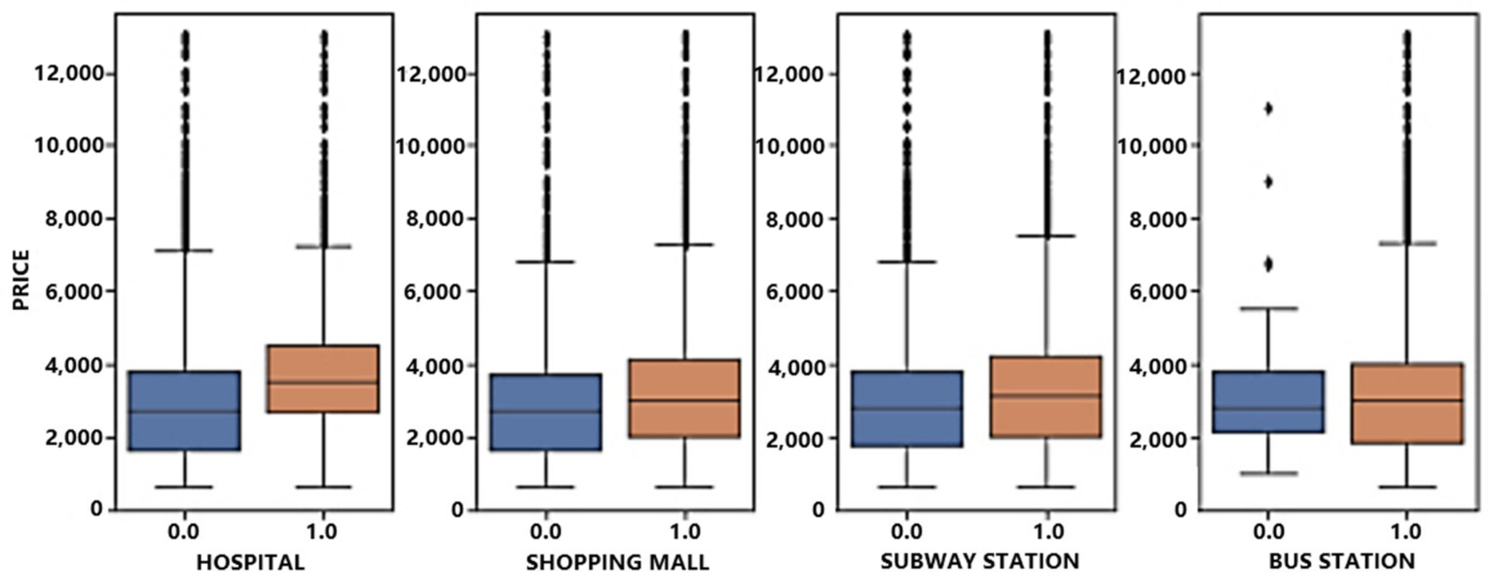
3.1.7. Data Visualization

In order to more intuitively display the data characteristics of each variable, data visualization is conducted after removing missing values and outliers. This approach enables further analysis of the relationship between each feature and the rental price.
First, we create a heatmap to depict the correlation between prices and various characteristics, as illustrated in Figure 3. The heatmap is drawn based on the correlation coefficient between feature variables including price (P), area (A), living room (L), orientation (O), elevator (E), toilet (T), supermarket (S), office building (O), park (P), subway (SB), bus (B), shopping mall (SM) and hospital (SM). This visualization facilitates a preliminary understanding of the relationships between different variables. The heatmap reveals a strong positive correlation between area and rental prices, while variables such as distance from the nearest hospital and the nearest shopping mall exhibit a negative correlation with rental prices. Further exploration of the impact of each variable’s different values on price is necessary. Simultaneously, it is essential to note that some variables exhibit a strong correlation, such as supermarkets and office buildings. Consequently, variable selection is required before modeling to avoid multicollinearity between variables.
To visually represent the changes in the distribution of dependent variables following logarithmization, we plot the probability density diagram and the QQ plot for rental prices before and after logarithmization, as depicted in Figure 4. The rental prices in the original dataset exhibit a substantial right-skewed distribution, which approaches a normal distribution after the logarithmic transformation.
To visually depict the distribution of property resources across various districts of Nanjing, a scatter plot of rent distribution is created, as presented in Figure 5. The plot demonstrates that property resources are primarily concentrated in central urban areas of Nanjing, including Jianye District, Xuanwu District, Qinhuai District, and Gulou District. The area without property resource distribution at the bottom of the figure is Gaochun District, which is not considered in this analysis.
The following box plots illustrate rental prices in different areas, as depicted in Figure 6. Overall, rental prices in various regions of Nanjing can be classified into the following three levels.
The first level comprises Jianye District, Xuanwu District, Qinhuai District, and Gulou District. The median rental prices in these regions range from 3000 to 4000 yuan per month. These areas are situated in the central urban area of Nanjing, characterized by a high concentration of shopping malls, financial technology companies, and office buildings. Consequently, there is substantial demand for rental properties. Notably, Jianye District exhibits a significant difference in its rent prices.
The second level includes Yuhuatai District, Jiangning District, Qixia District, and Pukou District, with median prices between 2000 and 3000 yuan per month.
The third level comprises Liuhe District and Lishui District. Due to their distance from the city center, the demand for rental housing is limited, resulting in lower rental prices.
Rental methods are also a crucial factor influencing housing prices. By plotting kernel density charts for joint and whole leases, we can compare the impact of different rental methods on prices, as illustrated in Figure 7 and Figure 8. The price of shared rent is concentrated between approximately 600 and 1600 yuan per month, while the price of homes with rent exceeding 2700 yuan per month is relatively rare. On the other hand, the price of whole rent is concentrated between 2000 yuan per month and 6000 yuan per month. Simultaneously, it can be observed that the prices of both rental methods exhibit a right-skewed distribution, underscoring the necessity for price logarithmization.
The orientation of a home directly determines its degree of lighting, comfort, and ventilation, thereby affecting the living experience. In this study, homes are categorized based on whether they face south or not. A box plot depicting the relationship between price and orientation is presented in Figure 9. It is evident that rental prices for south-facing homes are significantly higher than those of non-south-facing homes.
In addition to the basic attributes of a home that influence rental prices, nearby facilities and services also contribute to the added value of the property. In this analysis, we examine whether there are hospitals, shopping malls, subway stations, and bus stations within 1000 m, and plot a box chart, as depicted in Figure 10. The figure reveals that the price of properties with nearby medical, entertainment, and transportation services is higher than that of properties without these services. This finding reflects that people’s rental demands extend beyond merely comfortable living spaces; they also prioritize convenience and comprehensive services.

3.1.8. Variable Selection

Variable selection is an important step before establishing a model. Eliminating redundant variables helps preserve essential information while reducing training time and preventing model overfitting. Common feature selection methods can be categorized into the following three groups:
  • Filter: Features are first selected according to predefined criteria, followed by training the learner. These two parts do not influence each other.
  • Wrapper: After multiple training iterations, the model’s performance serves as an evaluation criterion for a subset of features. This method is more computationally intensive than filter-based approaches but offers better results.
  • Embedding: The initial step involves selecting a training set, followed by using the selected data to train the learner. This method integrates feature selection and model training processes, optimizing both selection and training simultaneously.
In this study, Recursive Feature Elimination (RFE) was selected for variable selection. RFE is a backward search algorithm based on the wrapper mode that uses a machine learning model to conduct multiple rounds of training to select the best feature subset to achieve the goal of feature selection. The algorithm follows these steps: first, all features are used to construct an initial feature set, and the model is trained on the feature set. This study selects the random forest model to calculate the importance of each feature variable and rank them. Next, the feature with the lowest importance is deleted, the model is trained on the new dataset, and the importance of each feature variable is calculated and sorted. Finally, the above steps are repeated until the optimal subset of feature variables is determined. The RFE-RF model flowchart is shown in Figure 11.
Using the RFE-RF method for variable selection, 14 important variables were ultimately selected from the original 30 variables, as shown in Table 6.

3.2. Model Implementation

3.2.1. Base Learners and Meta Learner

Our model GERPM selects random forest, XGboost, LightGBM and CNN as base learners, optimizes their parameters to achieve the optimal prediction, and then constructs a stacking ensemble learning model that integrates GWR as the meta learner.

Random Forest

Random forest (RF) [32] is an integrated learning algorithm based on decision trees, widely used in classification and regression problems due to its good prediction performance and ability to handle high-dimensional samples [33]. In the process of constructing a tree, unlike a general decision tree that traverses all features, a random forest model randomly selects some features from the feature set of the new sample set and then constructs a decision tree on the finally extracted sample set. Multiple decision trees form a random forest, with each decision tree not interfering with each other, performing parallel prediction. During the final prediction, the results of all decision trees are considered to reduce errors. The specific process steps of the algorithm are as follows:
Step 1: Through Bootstrap sampling, repeat K times to obtain K independent and identically distributed sample training sets, forming K trees in a random forest.
Step 2: Train the model on each sampling set, select m attributes by simple random sampling, select the best segmented attribute as a node based on information gain or Gini index, and split until further splitting is impossible. Based on this process, train multiple regression trees to form a random forest.
Step 3: Apply a random forest to the test set, use the voting method to obtain the predicted values for the classification task, and determine the predicted values using the mean method for the regression task.

LightGBM

LightGBM is a new Boosting framework model proposed by Microsoft in 2017, optimized based on the traditional GBDT model. Its principle is similar to that of the XGBoost model, with significant improvement in computational complexity [34]. It supports efficient parallel computing and runs faster with less memory consumption compared to the XGBoost model. LightGBM is improved through the following two strategies: gradient-based one-side sampling (GOSS) and exclusive feature binding (EFB). The gradient unilateral sampling technology assigns different weights to samples based on their gradient values during training, playing a different role in learning. Compared to uniform random sampling, it obtains more accurate information gain by preserving data with large gradient values. For data with small gradient values, random selection is used to avoid the impact of low-gradient long tail parts on the model while maintaining the consistency of sample distribution to a certain extent. The independent feature merging technology reduces the number of features by bundling mutually exclusive features to achieve dimensionality reduction without losing information. In high-dimensional data, data are often sparse, and many features are mutually exclusive. The basic idea of this technology is to discretize continuous features, construct a histogram, count the cumulative statistics of each discrete value in the histogram, and search for the optimal segmentation location based on the histogram during feature splitting. This method reduces the storage space of the original data while preventing overfitting. Through the above two technologies, LightGBM has greatly saved time, reduced energy consumption, and achieved outstanding practical results in the industry.

XGBoost

Extreme Gradient Boosting (XGboost) is a boosting integration algorithm based on decision trees, first proposed and used by Chen T. [35] in 2016. It uses the lifting tree principle to carry out multiple iterations during the training process and improves the solution by using the second derivative information of the loss function. Based on GBDT, XGBoost use the negative gradient of the model on the data as an approximation of the residual to fit the residual. It uses Taylor expansion to approximate the loss residual of the model, adds regularization terms, and effectively avoids the overfitting problem of the model with high computational accuracy and strong classification accuracy.
The basic idea of XGBoost is to extract a part of the variables each time to construct a regression tree model and repeat the process. Finally, multiple regression tree models are obtained and linearly combined, forming an additive model used to form the basic tree model to obtain the final result. Assuming that K trees are trained, the prediction result of the i -th sample is shown in Equation (3).
y ^ i = n = 1 k f n ( x i )
where x i is the sample feature, and f k ( x i ) is the prediction of the k -th tree on the sample. The accumulation of each result is the final prediction value y . Considering the complexity of the model and the accuracy of the results, the objective function consists of two parts, and the equation is shown in (4) and (5):
o b j = i = 1 n l ( y i , y ^ i ) + k = 1 Ω ( f k )
Ω f = γ T + 1 2 λ w 2
The first part is the loss function, and the second part is the regularization term. The symbol T represents the number of leaf nodes, and γ controls its number. The symbol w represents the score of the leaf node, and λ ensures that the score is not too large to constrain the complexity of the model and improve the generalization ability of the model. To minimize the objective function, Taylor expansion is used to approximate the objective function and delete the constant term in the formula, which simplifies the objective function to Equation (6).
L ˜ ( k ) = i = 1 n [ g i f k ( x i ) + 1 2 h i f k 2 ( x i ) ] + Ω ( f k )
where g i and h i are the first and second derivatives of the loss function of the i -th decision tree, respectively, transferring the loss information predicted by the previous k 1 -th decision tree to the k -th tree. The XGBoost model has obvious advantages and is widely used in data science analysis and data mining competitions due to its excellent prediction accuracy.

CNN

Convolutional Neural Networks (CNN) [36,37,38,39] are a type of feedforward neural network that extract the structural features hidden in the data by convolution and pooling operations [39], avoiding the complex feature extraction process with less manual participation. They are composed of an input layer, hidden layer and output layer, with the hidden layer structure being more complex and important, including a convolutional layer, pooling layer, and fully connected layer. The input layer preprocesses the data to reduce the impact of data dimensions. Convolutional layers are used to extract data features, with the most important being the convolution kernel. The number, shape, and size of the convolution kernel need to be determined, with larger kernels extracting more complex features. Step size refers to the distance of each movement calculated by convolution. The role of the pooling layer is to reduce dimensions. If the convolution operation makes the space of the output feature data too large, the pooling layer can compress the feature information of the feature data, reduce the data space, reduce the number of parameters, and facilitate model optimization. The fully connected layer maps features to the sample marker space, with each neuron connected to the previous layer of neurons for linear combination, improving the model’s prediction ability and transferring data information to the next layer of the network. The output layer inputs the output value of the fully connected layer into the activation function to obtain the final output of the neural network, which is the non-linear transformation result of the neural network’s non-linear mapping. Convolutional neural networks have fewer parameters and are not prone to overfitting. At the same time, their generalization ability has been improved, and their adaptability is strong, allowing their use in various application scenarios for prediction.

Meta Learner

The GERPM model uses a Geographic Weighted Regression (GWR) model as the meta learner. GWR is a linear regression modeling method for spatial variation relationships. Compared to traditional linear regression, geographic weighted regression models introduce the distance weight function of spatial location into the regression equation and incorporate spatial changes into the parameter estimation of explanatory variables in the model, while adding spatial vector data to the equation model [40]. Compared to general linear regression models, the GWR model considers the location information of observation points, performs linear regression for sample points at different geographical locations, and calculates the coefficient results of the impact of various factors on housing prices. It fully considers the local effects of spatial objects, reveals spatial heterogeneity, and improves the accuracy and explanatory power of the results. This model allows different relationships between different points in space and allows parameters to change in space, as shown in Equation (7).
y i = β 0 ( u i , v i ) + j = 1 k β j ( u i , v i ) x i j + ε i
where y i is the housing price of the sample; u i ,   v i represents the spatial geographic coordinates of the i -th sample; β j u i ,   v i is the j -th regression coefficient of the i -th sample; x i j is the value of variable x j at sample i ;   ε i is an independent and identically distributed random error term.
The GWR model uses the weighted least-squares method to estimate parameters, which depends on spatial location and estimates local parameters rather than global parameters. Among them, determining the spatial weight matrix is the most critical step, which reflects an individual’s dependence in space. The weight function is used to measure the strength relationship between sample points at different locations. Common spatial weight functions include the distance threshold method, Gaussian function method, inverse distance method, etc. In this study, the Gaussian kernel function method is used to determine spatial weight. When performing parameter estimation on regression point i , points near i are given greater weight as shown in Equation (8).
W i j = exp ( ( d i j / b ) 2 )
where w i j represents the regression weight value between the i -th data point and the j -th sample; d i j represents the distance between the i -th data point and the regression point; b represents the bandwidth or number of adjacent points.
The size of the bandwidth or adjacent number of points determines the rate of change in the weight on the spatial scale. The larger the bandwidth or adjacent number of points, the slower the weight decays with distance. The commonly used bandwidth calculation methods include Cross-Validation (CV) and Akaike Information Criterion (AIC). In this study, the minimum information criterion method is used to determine the optimal bandwidth, as shown in Equation (9).
A I C = 2 K 2 ln L
where K is the number of parameters, and L is the likelihood function of the model. The smaller the parameter value, the simpler the model, and the smaller the AIC value. The larger the maximum likelihood function value, the more accurate the model, and the smaller the AIC value. The AIC evaluation combines simplicity and accuracy.

3.2.2. Parameter Tuning

Parameter tuning is crucial for improving the performance of the model. In this study, we conducted comprehensive parameter optimization and analyzed the impact of different parameters on the model’s performance. In the subsequent sections, we will provide a detailed discussion on the methods and process employed for parameter tuning, along with an exploration of the effects of different parameters.

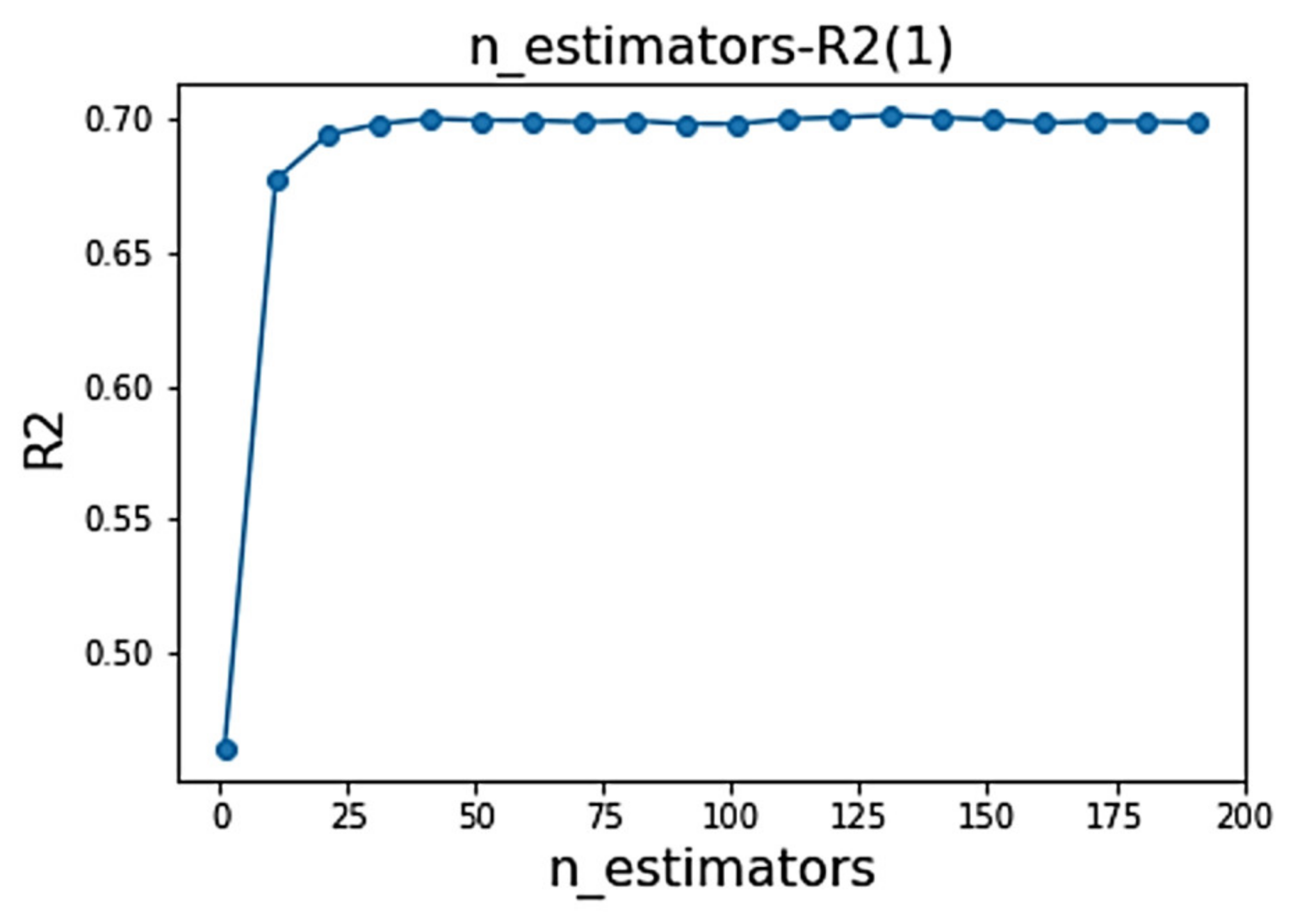
Random Forest Model Parameter Tuning

In this study, a simplified Grid Search Method (GSM) is used to optimize the parameters of the random forest model to improve the efficiency of parameter optimization. The GSM is a common parameter optimization method that includes an objective function, a search range, and other factors. The grid search traverses all combinations of internal parameters of the algorithm, lists all value combinations of all the variables one by one, and filters out the optimal parameter combinations through evaluation index scores, making it highly possible to find the global optimal value. However, as the number of parameters increases, the number of combinations of variable values also increases rapidly, consuming a large amount of calculation time. In this study, we first perform a grid search on each parameter, calculate the value with the highest score for that parameter, sort the scores for each parameter, add the parameter with the highest score to the model, and continue the grid search on it based on the current model. If the remaining variables can improve their scores, they are added to the model, otherwise the parameter adjustment stops. For parameters with a large search range, they can be optimized twice to obtain the best parameters. For example, in the first step, 10 can be taken as the step size to narrow the search range, and in the second step, 1 can be taken as the step size to determine the best parameters. At the same time, the grid search method is often combined with cross validation to find hyperparameters. Each evaluation index is calculated using the cross-validation method. Taking a 5-fold cross validation as an example, first, we divide the sample into five equal parts, select one part as the test set, and the remaining four parts as the training set. Use the training set to train a model, we can apply the trained model to the test set, and calculate the evaluation index score. Next, we repeat the above process until all samples are taken as a test set, obtaining five scores, which are averaged to produce the final score.
According to the grid search method, the main parameters of the random forest are optimized as follows:
  • n_estimators—the number of decision trees, which is also the iteration number of weak learners;
  • max_features—the number of randomly selected features for each decision tree;
  • min_samples_split—the minimum number of samples required to split internal nodes;
  • min_samples_leaf—the minimum number of samples that should be present on a leaf node.
The specific optimization process is as follows. Taking the n_estimators parameters as an example, R 2 is set as the evaluation index. After five-fold cross validation, R 2 values under different parameter values are obtained. The first optimization search range is (0, 200), with a step size of 10. The obtained parameter value is 131, and the corresponding R 2 is 0.7. Based on this, the optimal parameter range is determined to be (120, 140), as shown in Figure 12. Therefore, for the second time, a grid search is established with a search range of (120, 140) and a step size of 1 to determine the optimal parameter. At this step, the optimal parameter is found to be 120, with an R 2 of 0.702, as shown in Figure 13.
The results of single parameter optimization for the random forest model are shown in Table 7.
From the results of optimizing a single parameter, it can be observed that the optimization of different parameters improves the prediction effect of the model to varying degrees. Next, based on the ranking of R 2 values, the parameters including max_features, max_depth, n_estimators, min_samples_split, and min_samples_leaf are sequentially added to the model training to obtain the final parameters and their corresponding R 2 values, as shown in Table 8.

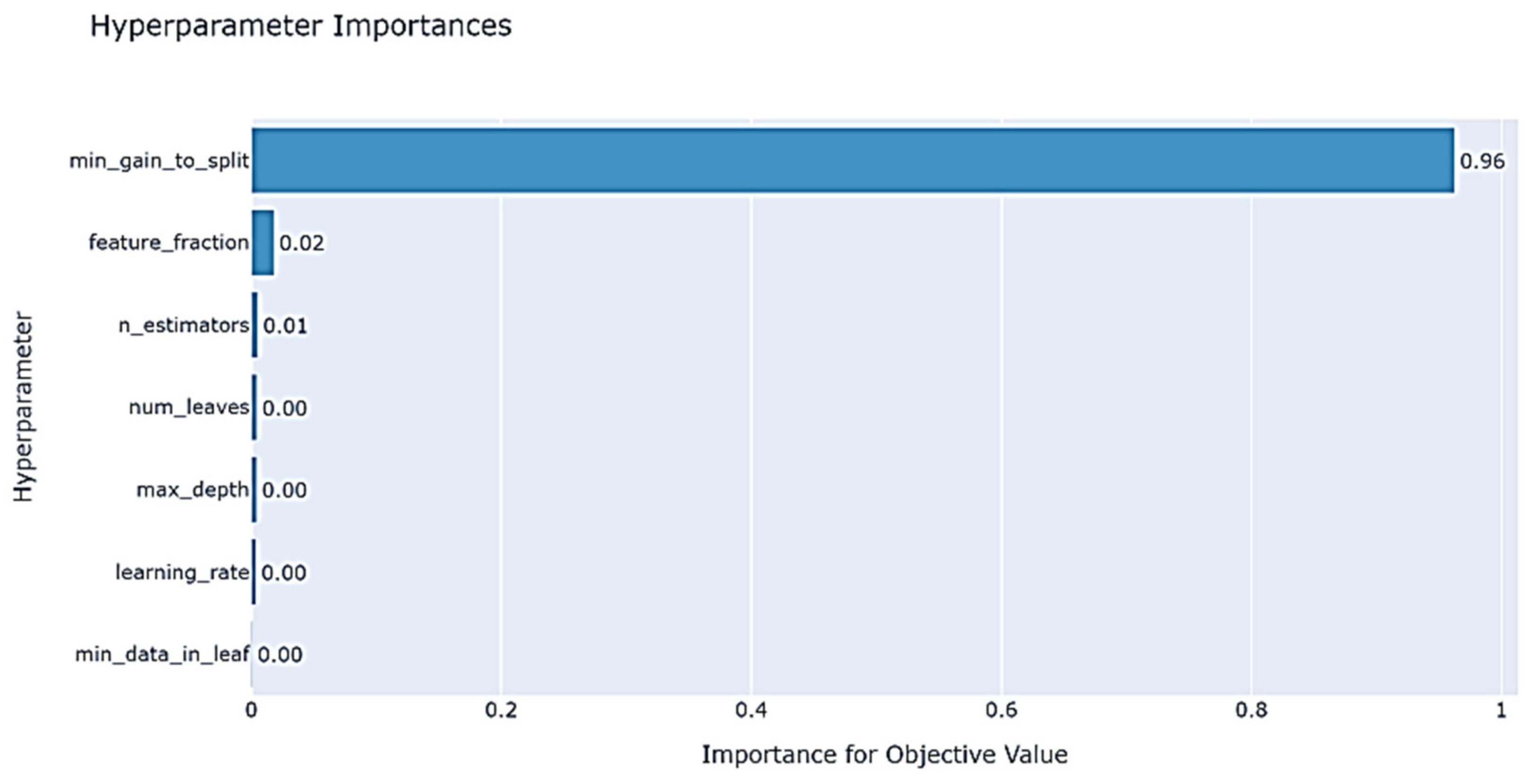
LightGBM Model Parameter Tuning

For the LightGBM model, this study selects the Optuna framework for parameter tuning. Optuna describes hyperparameters as the process of maximizing/minimizing an objective function that takes a set of hyperparameters as input and returns a verification score. Its essence is to determine the optimal hyperparameters based on Bayesian probability and iteratively adjust the search. It is a trial and error algorithm based on improved Bayesian probability and has good stability. Optuna uses more computational power in areas with higher probability by predicting parameter intervals with lower probability of termination, thus reducing a significant amount of wasted computational power on invalid combinations. When the effectiveness of searching for a certain area becomes worse and the loss no longer decreases, the search for that area is stopped. Finally, the optimal area is selected, which improves the search efficiency.
To optimize the parameters of the LightGBM model, the following parameter settings are used:
  • n_estimators: trial.suggest_int (“n_estimators”, 100, 2000, step = 10)—the number of iterations, selected based on the characteristics of the dataset, with a search range of (100, 2000).
  • learning_rate: trial.suggest_float (“learning_rate”, 0.01, 0.2)—learning rate, controlling the convergence speed, with a search range of (0.01, 0.2).
  • max_depth: trial.suggest_int (“max_depth”, 3, 10)—the maximum depth of the tree model, the most important parameter to prevent overfitting and has a significant impact on model performance, with a search range of (3, 10).
  • num_leaves: trial.suggest_int (“num_leaves”, 20, 3000, step = 20)—the number of leaf nodes on a tree, working with max_depth to control the shape of the tree, with a search range of (20, 3000).
  • min_data_in_leaf: trial.suggest_int (“min_data_in_leaf”, 10, 100, step = 10)—the minimum amount of data on a leaf, with a search range of (10, 100).
  • min_gain_to_split: trial.suggest_float (“min_gain_to_split”, 0, 15)—the minimum gain threshold for splitting, with a search range of (0, 15).
  • feature_fraction: trial.suggest_float (“feature_fraction”, 0.2, 0.95, step = 0.1)—randomly selects the feature ratio in each iteration, with a search range of (0.2, 0.95).
The number of experiments is set to 100, and the optimal parameter values from the running results are shown in Table 9:
We can visualize the optimization process of Optuna by using the optuna.visualization library in Python. The function optional.visualization.plot_slice (study, params = [‘hyperparameters’]) is used to view the values of different hyperparameters in the experiment, visually displaying the target values corresponding to different hyperparameter value combinations. This provides a visual reference for setting the hyperparameter range when optimizing the model, as shown in Figure 14 and Figure 15, reducing the trial and error of ineffective parameters. For example, the learning_rate values are concentrated between 0 and 0.1, n_estimators values are concentrated between 500 and 1100 and max_depth values are concentrated from 6 to 8.
The function plot_parallel_coordinated (study) shows the overall optimization process of combining different superparametric values, as shown in Figure 16.
The function optuna.visualization.plot_param_Importances (study) shows the significant impact of hyperparameters on the overall model, as shown in Figure 17. It can be observed that min_gain_to_split has the most significant impact on the effectiveness of the LightGBM model.
During the parameter optimization process, there are many invalid parameter combinations. Optimizing such combinations will increase computational complexity. Early termination can save time and improve the efficiency of model optimization. Optuna has a built-in pruning algorithm that largely solves the problem of invalid parameter combinations. The function optuna.visualization.plot_optimization_history (study) shows the historical process of parameter optimization. It can be observed that the optimization interval of Optuna is concentrated between 0.227 and 0.24, with few optimization combinations above 0.24. The specific optimization process is shown in Figure 18.

XGBoost Model Parameter Tuning

The XGBoost model parameters are also optimized using the Optuna framework, with the following parameter settings:
  • learning_rate: trial.suggest_categorical (‘learning_rate’, (0.008, 0.009, 0.01, 0.012, 0.014, 0.016, 0.018, 0.02))—the learning rate, controlling the convergence rate. After the experiments, the learning rate search range is determined to be between 0.01 and 0.02.
  • n_estimators: trial.suggest_int (“n_estimators”, 1,002,000, step = 10)—the number of iterations, selected based on the characteristics of the dataset, with a search range of (100, 2000).
  • max_depth: trial.suggest_categorical (‘max_depth’, [3, 6, 9, 12, 15, 18, 21, 24])—the maximum depth of a tree model, the most important parameter to prevent overfitting, and has an important impact on model performance. The search range for max_depth is from 3 to 25 in terms of integers.
  • min_child_weight: trial.suggest_int (‘min_child_weight’, 1, 100)—the minimum sample weight sum in the leaf node. If the sum of sample weights for a leaf node is less than min_child_weight, the split process ends. The search range is (1, 100).
After setting the parameter range, the mean square error is used as the return value for tuning. The parameter direction of the study function is set to “minimize”, meaning that the smaller the mean square error, the better the prediction effect. The number of experiments is set to 100, and the optimal parameter values from the running results are shown in Table 10.
The function optuna.visualization.plot_slice (study, params = [‘hyperparameters’]) intuitively displays the target values corresponding to different hyperparameter value combinations’ landing points. This provides a visual reference for setting the hyperparameter range when optimizing the model, as shown in Figure 19, and reducing invalid parameter trial and error. For example, min_child_weight values are concentrated between 0 and 50 and n_estimators values are concentrated between 1400 and 2000.
The function plot_parallel_coordinate (study) shows the overall optimization process of combining different hyperparameter values, as shown in Figure 20.
The function optuna.visualization.plot_param_importances (study) shows the significant impact of hyperparameters on the overall model, as shown in Figure 21. It can be observed that n_estimators have the most significant impact on the XGBoost model.
The function plot_optimization_history (study) shows the historical process of parameter optimization, showing that the optimization interval of Optuna is concentrated around 0.2. The specific optimization process is shown in Figure 22.

CNN Model Parameter Tuning

The important parameters of CNNs (Convolutional Neural Networks) are as follows:
  • Activation function of neurons: The activation function enables neural networks to have the ability to perform non-linear prediction. It converts the results of each layer of neural networks after linear calculations into non-linearities. The ReLU function has the ability to zero out the output of certain neurons, thereby suppressing overfitting.
  • Dropout Layer: During the training process of the neural network, some neurons are randomly selected for deletion to suppress overfitting.
  • Batch_size: The batch size refers to the amount of data randomly input during each iteration of neural network training. If the batch size is too small, gradient updates are too slow, and while if it is too large, the global optimal solution becomes difficult to determine.
  • Epoch: Completing a round of learning using all the data is known as completing the training process. Increasing the number of epochs is conducive to iteratively adjusting the weight parameters of the model towards their optimal value.
  • Loss Function: The model parameters are updated by calculating the model’s error during the training process. This study employs the mean square as its loss function.
  • Optimizer: A neural network with multiple layers and parameters may require a significant amount of time to train. To accelerate the training process, different optimizers provide different optimization paths based on their respective principles. Selecting an appropriate optimizer can reduce the training time and improve the overall training efficiency. This study utilizes the Adam optimizer with a learning rate of 0.001.
The primary parameters of the CNN are optimized using the grid search method, and the optimization results are presented in Table 11.
In this study, we design and build a CNN network model consisting of three convolutional layers. For each layer, the model uses 32 convolutional kernel filters with a kernel size of 3. The model also incorporates a max-pooling layer, and its fully connected layer contains 128 neurons.

3.2.3. Constructing an Ensemble Learning Model Based on Stacking

Analysis of Spatial Autocorrelation

Traditional hedonic price models generally assume that variables are homogeneous. However, in real-life scenarios, the relationship between variables may vary due to different spatial locations. Therefore, when analyzing spatial data, it is necessary to consider spatial non-stationary characteristics and determine modeling strategies [41]. The Moran [42] Index is a quantitative measure of spatial heterogeneity, which can be divided into the global Moran’s Index and local Moran’s Index. The term “narrow” Moran Index typically refers to the global Moran’s Index.
(1) Global spatial autocorrelation
Global autocorrelation measures the overall average degree of aggregation within a region and is often quantified using Moran’s I, as shown in Equation (10).
I = n i = 1 n j = 1 n w i j × i = 1 n j = 1 n w i j ( x i x ¯ ) ( x j x ¯ ) i = 1 n ( x i x ¯ ) 2
where n represents the number of samples, x i , x j represent the attribute values of sample points i and j , respectively, and w i j represents the spatial weight matrix. Following the variance normalization process, Moran’s I index has a value range of [−1,1]. A Moran’s I value greater than 0 suggests positive spatial correlation, meaning that regions with similar high or low attributes tend to cluster together. Conversely, a Moran’s I value less than 0 indicates negative spatial correlation, meaning that regions with different attribute values cluster together. When Moran’s I is equal to 0, the data exhibit spatial randomness.
The global Moran’s Index for home rental prices in Nanjing, calculated using the R moran function, is 0.24, indicating a strong positive correlation with geographical distribution. The results of the global autocorrelation test are shown in Figure 23 and indicate that the probability of randomly generating this clustering result is less than 1%. In other words, home rental prices in Nanjing have passed the significance test, demonstrating a significant spatial clustering effect in space.
(2) Local spatial autocorrelation
Local autocorrelation reflects the spatial clustering of individual regions and analyzes the similarity between each unit and its adjacent spatial locations, thereby identifying spatial clustering patterns at the local level. The Moran scatterplot is the primary way to present local spatial correlation analysis. The equation for calculating the local Moran’s Index is shown in Equation (11).
Z ( I ) = n ( x i x ¯ ) j i n w i j ( x j x ¯ ) i = 1 n ( x i x ^ ) 2
where w i j represents the spatial weight matrix, x i , x j represent the attribute values of sample points   i   and j , and x ¯ is the average value of sample point attributes. We utilize R language to draw a local Moran’s Index scatterplot of rental prices in Nanjing, as shown in Figure 24.
According to the local Moran’s Index scatterplot, the points in the first and third quadrants are higher than those in the second and fourth quadrants, indicating that properties with higher or lower rental prices are more likely to gather spatially. Therefore, it is possible to construct a GWR model for the rental price data in Nanjing.

Building a Stacking Ensemble Learning Model

Stacking Ensemble Learning is a machine learning algorithm proposed by Wolpert in 1992. It combines different types of algorithms, often achieving significantly superior generalization performance than an individual algorithm [43]. Generally, it is designed as two layers. The first layer uses training set data to train base learners. Then, in the second layer, meta learners use the results of the previous layer’s predictions to complete model construction. To avoid over fitting, we use K-fold cross-validation on training data before building the model. This helps to increase the stability and reliability of the model. The specific steps are as follows:
Step 1: Divide the training set and test set.
Step 2: Divide the training set into K parts, take out one part, and use the remaining K-1 parts of the training model to predict the value of the extracted data. Each time during K-fold cross-validation, the model is also used to predict the target values of the test set. The predicted values are then averaged over the K iterations to obtain a more reliable estimate of the model’s performance on unseen data. Repeat this step to obtain K predictions.
Step 3: Set a total of n base learners. Repeat the above steps for each base learner model to obtain n-dimensional data, input it to the meta learner model, and obtain the final prediction result.
In this study, our model GERPM uses 5-fold cross-validation to construct a stacking ensemble learning model that integrates GWR; the first layer of base learners is the random forest model, XGBoost model, LightGBM model, and CNN model after tuning parameters, and the second layer of meta learners is the GWR model. Its structure is shown in Figure 25.
This study uses the R language’s GWmodel package to build a geographically weighted regression model. Firstly, the bandwidth is calculated using the bw.gwr function, and the AIC method is selected as the calculation method. Then, a geographic weighted regression model is constructed using Gaussian kernel functions. The results are shown in Figure 26. The results show that the number of adjacent points is 363, that is, using the latest 363 sample points for parameter estimation. Among the four base learners, the second model, LightGMB, has the best prediction performance and exerts the most significant impact on the final prediction. The final model exhibits a goodness of fit prediction of 0.87 on the test set.

4. Results and Analysis

4.1. Evaluation Metrics

Mean Squared Error (MSE): An indicator that reflects the degree of difference between the actual value and the predicted value. The smaller the value is, the smaller the error is, and it often used as a loss function, as shown in Equation (12).
M S E = 1 m i = 0 m y ^ i y i 2
Root Mean Squared Error (RMSE): The square root of the mean square error. The smaller the value is, the more accurate the prediction is, as shown in Equation (13).
Z ( I ) = n ( x i x ¯ ) j i n w i j ( x j x ¯ ) i = 1 n ( x i x ^ ) 2
Coefficient Of Determination ( R 2 ): The value is usually between (0, 1). The closer R 2 is to 1, the closer the predicted value of the model is to the real value, the stronger the explanatory power of the model for dependent variables is, and the better the fitting effect, as shown in Equation (14), where y i represents the actual value, y ¯ represents the sample average, and y i ^ represents the predicted value.
R 2 = 1 i = 1 m ( y ^ i y i ) 2 i = 1 m ( y i y ¯ ) 2

4.2. Prediction Results Comparison and Analysis

The stacking ensemble learning model GERPM with GWR as the meta learner improves the prediction performance of machine learning while considering the influence of geographical location on rental prices. In order to verify its prediction performance, the results are compared with those of the individual models (RF, LightGBM, XGBoost and CNN), the equal weight combination model, and the stacking ensemble learning model with multiple linear regression as the meta learner, i.e., stack (OLS). Among them, the equal weight method is a combination model method that assigns the same weight to each model. It treats all models equally, regardless of priority. The weight of each model is 1 / k , and k is the number of models. For the stacking ensemble learning model with multiple linear regression, the first layer of base learners consists of four machine learning models after parameter tuning, and the second layer of the meta learner consists of the multiple linear regression model. The comparison of the predicted results of rental prices in Nanjing by various models is shown in Table 12.
It can be observed that the equal weight method model and the stacking ensemble learning models have better prediction performance than the individual model. GERPM as a stacking ensemble learning model integrating GWR has achieved the best prediction performance on MSE, RMSE and R 2 . Compared with stacking (OLS) without considering geographical location, R 2 increased from 0.858 to 0.87, an increase of 2.4%, and MSE decreased from 0.052 to 0.047, a decrease of 9.6%. Compared with the average prediction results of an individual model, R 2 increased by 19.2% from 0.73 to 0.87, and MSE decreased by 35.6% from 0.073 to 0.047. Therefore, GERPM significantly reduces prediction errors and improves the prediction accuracy of the model.

4.3. Robustness Analysis

The GERPM model has achieved good results in predicting rental prices in Nanjing. To compare the prediction performance and analyze the robustness of the model, relevant data on home rental information in Shanghai and Hangzhou were obtained for experimentation.

4.3.1. Prediction Results of Residential Rents in Shanghai

As an economic and financial center, Shanghai has provided a large number of employment opportunities, attracting entrepreneurs and staff from all over the world. The permanent resident population has reached over 24 million, driving a significant demand for home renting. In this research, there are real data of rental prices and home attributes in Shanghai. The POI data near the properties are obtained from the Baidu Maps open platform, and the population and economic data of each district of Shanghai are obtained through the Shanghai Statistical Yearbook provided by the Shanghai Municipal Bureau of Statistics. A total of 14,759 valid data samples are obtained. We draw the probability density map of Shanghai’s rental price, as shown in Figure 27. The probability density map of Shanghai’s rental price is obviously skewed to the right, requiring logarithmic processing. After data preprocessing such as missing values, outliers, and logarithmic dependent variables, a total of 28 variables are obtained for RFE-RF variable selection, and finally, the following 13 variables are retained, as shown in Table 13.
To test the spatial autocorrelation of rental prices in Shanghai, the global Moran’s Index was calculated to be 0.53, with a significant p-value at the 0.01 level, indicating a positive correlation between prices and geographical distribution, and a significant spatial clustering effect in space. The grid search method is used to tune the parameters of the random forest and CNN models, and the Optuna framework is used to tune the parameters of XGBoost and LightGBM. The model parameters are shown in Table 14, Table 15, Table 16 and Table 17.
The models with optimized parameters are used to predict rental prices in Shanghai, and then the above models were combined using the equal weight method, stacking ensemble learning method with multiple linear regression, and GERPM, and the results are shown in Table 18.
After comparing the prediction results of various models (Shanghai) as shown in Table 18, it was found that GERPM had the most accurate predictions with the lowest values for MSE and RMSE, and the highest R 2 score among all the models. Compared with the prediction results of stacking (OLS), R 2 increased by 1.8% from 0.927 to 0.944, and MSE decreased by 20% from 0.02 to 0.016. Compared with the average prediction results of an individual model, R 2 increased by 22% from 0.773 to 0.944, and MSE decreased by 76% from 0.063 to 0.016. Therefore, GERPM significantly reduces prediction errors and improves the prediction accuracy of the model. Compared to Nanjing, GERPM has significantly improved the prediction effect of rental data in Shanghai, which is closely related to the spatial clustering of rental prices in Shanghai. That is, the spatial clustering is strong, and the model’s prediction effect is good.

4.3.2. Prediction Results of Rental Prices in Hangzhou City

In recent years, Hangzhou City has leveraged the development opportunities of the Internet era and experienced significant growth by capitalizing on the e-commerce industry. At the same time, it actively carries out effective talent introduction policies to attract population inflows, and the population continues to grow. The rental market is experiencing a strong trend of growth and development. In this research, there are real data of rental prices and home attributes in Hangzhou. The Baidu Maps open platform is called to obtain the POI data near the homes, and a total of 31,771 valid data samples are obtained. Due to the adjustment of some administrative districts in Hangzhou in 2021, the statistical data of each district over the years deviated from the current actual region. To ensure the authenticity and effectiveness of the data, relevant population and economic data for each district are not obtained. We draw a probability density map of rental prices in Hangzhou, as shown in Figure 28. The probability density map of rental prices in Hangzhou shows a significant right deviation distribution, requiring logarithmic processing. After data preprocessing, including missing values, outliers, and logarithmization of dependent variables, 28 variables were obtained for RFE-RF variable selection, and the following 13 variables were retained, as shown in Table 19.
To test the spatial autocorrelation of rental prices in Hangzhou, the global Moran’s Index was calculated to be 0.2, with a significant p-value at the 0.01 level, indicating a positive correlation between prices and geographical distribution, as well as a significant spatial clustering effect in space. Furthermore, based on the local Moran scatterplot, there is a spatial clustering phenomenon of properties with either higher or lower rental prices in Hangzhou. The grid search method is used to adjust the parameters of the random forest and CNN model, and the Optuna framework is used to adjust the parameters of XGBoost and LightGBM. The model parameters are shown in Table 20, Table 21, Table 22 and Table 23.
The optimized models were used to predict the rental prices in Hangzhou, and the above models were combined using the equal weight method, stacking ensemble learning method with multiple linear regression as the meta learner, i.e., stacking (OLS), and GERPM. The comparison of the results is shown in Table 24.
It can be observed that the prediction accuracy of individual models in Hangzhou is relatively lower compared to those of Nanjing and Shanghai. This is closely related to the lack of regional economic and demographic data in Hangzhou’s dataset, which underscores the significant impact of regional economic and social development on rental prices. Compared with the prediction effect of the individual models, the combination of multiple models has significantly improved the fitting accuracy. Among them, the GERPM has the best prediction performance and the smallest prediction error. Compared with the predicted results of stacking (OLS), R 2 increased by 6.5% from 0.79 to 0.84, and MSE decreased by 32.5% from 0.083 to 0.056. Compared with the average prediction results of the individual models, R 2 increased from 0.773 to 0.84, an increase of 32.7%, and MSE decreased from 0.063 to 0.056, a decrease of 53%. The stacking (GWR) model has still achieved optimal prediction results in the prediction of Shanghai and Hangzhou’s residential rents, indicating that the model can achieve good prediction results in multiple cities and has good robustness.

4.4. Summary

In this section, we analyzed the prediction results and robustness of GERPM. In order to better evaluate the model’s prediction performance, we compared the prediction results with those of the individual model, the equal weight combination model, and the stack ensemble learning model with multiple linear regression as the meta learner. The comparison results indicate that our model has achieved the best prediction performance on the MSE, RMSE, R2 and other evaluation metrics of rental prices in Nanjing, significantly improving the prediction accuracy. To verify the robustness of the model, besides Nanjing, the data related to rental prices in Shanghai and Hangzhou were also obtained. Through the comparison of results, it was found that GERPM also achieved the best prediction results on the datasets of both cities, indicating that the model not only has good prediction performance but also strong robustness. These findings suggest that this model can be applied to rental prices prediction research in multiple cities.
The variables that are common among the three cities include area, number of bedrooms, distance to the nearest subway station, distance to the nearest shopping mall, distance to the nearest hospital, presence of an elevator, and whether the property is well decorated. These findings suggest that the area, unit type, elevator facilities, decoration, transportation, entertainment, and medical services around the home are very important factors that affect rental prices. Both Nanjing and Shanghai have included the economic population variable in their analysis. However, due to adjustments made to some administrative district divisions in Hangzhou, the statistical data deviated from the actual districts. As a result, the economic population variable was not included in the analysis. The results showed that the predicted results of Nanjing and Shanghai were better than those of Hangzhou, indicating that the economic population variable in the region is a factor that cannot be ignored in affecting rental prices.
To verify the robustness of the model, we obtained data related to rental prices in both Shanghai and Hangzhou. Through model prediction performance and comparison of results, it was found that the GERPM model still achieved the best prediction results on the datasets of these two cities, indicating that the model not only has good prediction performance but also strong robustness, and can be applied to rent prediction in multiple cities.

5. Conclusions

This paper presents GERPM, a novel urban residential rents prediction model based on geographically weighted stacking ensemble learning. GERPM comprehensively analyzes the factors influencing residential rents from multiple perspectives and utilizes the geographically weighted stacking ensemble learning method for prediction. The model combines multiple machine learning and deep learning models and achieves optimal predictions through parameter optimization. It not only fully leverages the advantages of deep learning and machine learning models but also incorporates a geographically weighted regression model to consider spatial heterogeneity. It effectively captures the spatial heterogeneity and geographical importance of rent prices and outperforms individual models and ensemble models that do not consider geographical factors. Experimental results in multiple cities validate the robustness and effectiveness of GERPM in predicting rental prices. Although GERPM has demonstrated great potential in accurately predicting urban residential rents, there are still some potential limitations and future research directions. Firstly, this study only covers rental data from a few cities in China. Future studies can expand the coverage of the dataset to include more cities and international data to enhance the model’s generalizability and adaptability. Additionally, the regional division can be further refined, and relevant features of different regions can be explored and measured, which would be another direction for our future work. Furthermore, in future studies, it would be beneficial to explore the semantic heterogeneity and similarity between model parameters. Thus, the model may gain a deeper understanding of the underlying factors influencing residential rents and further improve prediction accuracy.

Author Contributions

Conceptualization, G.H.; Formal analysis, G.H. and Y.T.; Investigation, G.H. and Y.T.; Methodology, G.H. and Y.T.; Project administration, G.H.; Resources, G.H.; Software, G.H. and Y.T.; Supervision, G.H.; Validation, G.H.; Visualization, Y.T.; Writing—original draft, G.H. and Y.T.; Writing—review and editing, G.H. and Y.T. All authors have read and agreed to the published version of the manuscript.

Funding

This research received no external funding.

Data Availability Statement

Not applicable.

Acknowledgments

We would like to extend our appreciation to Xin Fang, Jingqing Bao, and Tanyu Chen for their assistance during the revision process of this paper.

Conflicts of Interest

The authors declare no conflict of interest.

References

  1. Rajan, U.; Seru, A.; Vig, V. The failure of models that predict failure: Distance, incentives, and defaults. J. Financ. Econ. 2015, 115, 237–260. [Google Scholar] [CrossRef]
  2. Neloy, A.A.; Haque, H.M.S.; Islam, M.M.U. Ensemble Learning Based Rental Apartment Price Prediction Model by Categorical Features Factoring. In Proceedings of the 2019 11th International Conference on Machine Learning and Computing, Zhuhai, China, 22–24 February 2019. [Google Scholar]
  3. Zhang, X.Y. Rent Prediction Based on Stacking Regression Model and Baidu Map API. Master’s Thesis, Lanzhou University, Lanzhou, China, 2022. [Google Scholar]
  4. Henderson, J.V.; Ioannides, Y.M. A Model of Housing Tenure Choice. Am. Econ. Rev. 1983, 73, 98–113. [Google Scholar]
  5. Ioannides, Y.M.; Rosenthal, S.S. Estimating the Consumption and Investment Demands for Housing and Their Effect on Housing Tenure Status. Rev. Econ. Stat. 1994, 76, 127–141. [Google Scholar] [CrossRef]
  6. Shen, H.; Li, L.; Zhu, H.; Liu, Y.; Luo, Z. Exploring a Pricing Model for Urban Rental Houses from a Geographical Perspective. Land 2021, 11, 4. [Google Scholar] [CrossRef]
  7. Zhai, D.; Shang, Y.; Wen, H.; Ye, J. Housing price, housing rent, and rent-price ratio: Evidence from 30 cities in China. J. Urban Plan. Dev. 2018, 144, 04017026. [Google Scholar] [CrossRef]
  8. Bin, J.; Gardiner, B.; Li, E.; Liu, Z. Multi-Source Urban Data Fusion for Property Value Assessment: A Case Study in Philadelphia. Neurocomputing 2020, 404, 70–83. [Google Scholar] [CrossRef]
  9. Li, H.; Wei, Y.D.; Wu, Y. Analyzing the private rental housing market in shanghai with open data. Land Use Policy 2019, 85, 271–284. [Google Scholar] [CrossRef]
  10. Valente, J.; Wu, S.; Gelfand, A.; Sirmans, C.F. Apartment rent prediction using spatial modeling. J. Real Estate Res. 2005, 27, 105–136. [Google Scholar] [CrossRef]
  11. Choi, S.J.; Kim, S. Why do landlords include utilities in rent? Evidence from the 2000 Housing Discrimination Study (HDS) and the 2002 American Housing Survey (AHS). J. Hous. Econ. 2012, 21, 28–40. [Google Scholar] [CrossRef]
  12. Han, L.; Wei, Y.D.; Yu, Z.; Tian, G. Amenity, accessibility and housing values in metropolitan USA: A study of Salt Lake County, Utah. Cities 2016, 59, 113–125. [Google Scholar]
  13. Song, W.X.; Ma, Y.Z.; Chen, Y.R. Spatial and temporal variations in home price sales and rental prices in Nanjing urban area and their influencing factors. Geosci. Prog. 2018, 37, 1268–1276. [Google Scholar]
  14. Liu, C. Research on the Influencing Factors and Prediction of Housing Prices in Beijing. Master’s Thesis, Dalian University of Technology, Dalian, China, 2019. [Google Scholar]
  15. Islam, M.D.; Li, B.; Islam, K.S.; Ahasan, R.; Mia, M.R.; Haque, M.E. Airbnb rental price modeling based on Latent Dirichlet Allocation and MESF-XGBoost composite model. Mach. Learn. Appl. 2022, 7, 100208. [Google Scholar] [CrossRef]
  16. Xie, Y.; Zhang, W.; Ji, M.Z.; Peng, J.; Huang, Y.H. Application analysis of housing month rent prediction based on XGBoost and LightGBM algorithms. Comput. Appl. Softw. 2019, 36, 151–155. [Google Scholar]
  17. Liang, R. Based on Machine Learning Model Research on Housing Rent in Shenzhen. Master’s Thesis, Huazhong Normal University, Wuhan, China, 2020. [Google Scholar]
  18. Liu, S.Y. Machine Learning Methods for Analyzing the Influencing Factors of Urban Rental Prices. Master’s Thesis, Nankai University, Tianjin, China, 2021. [Google Scholar]
  19. Kang, Y.; Zhang, F.; Peng, W.; Gao, S.; Rao, J.; Duarte, F.; Ratti, C. Understanding house price appreciation using multi-source big geo-data and machine learning. Land Use Policy 2021, 111, 104919. [Google Scholar] [CrossRef]
  20. Wang, X.; Wen, J.; Zhang, Y.; Wang, Y. Real estate price forecasting based on SVM optimized by PSO. Optik 2014, 125, 1439–1443. [Google Scholar] [CrossRef]
  21. Tang, X.B.; Zhang, R.; Liu, L.X. Research on Prediction of Second-hand House Prices in Beijing Based on Bat Algorithm SVR Model. Stat. Res. 2018, 35, 71–81. [Google Scholar]
  22. Aziz, M.A.; Nurrahim, F.; Susanto, P.E.; Windiatmoko, Y. Boarding House Renting Price Prediction Using Deep Neural Network Regression on Mobile Apps. arXiv 2020, arXiv:2101.02033. [Google Scholar]
  23. Wang, P.Y.; Chen, C.T.; Su, J.W.; Wang, T.Y.; Huang, S.H. Deep learning model for house price prediction using heterogeneous data analysis along with joint self-attention mechanism. IEEE Access 2021, 9, 55244–55259. [Google Scholar] [CrossRef]
  24. Schmidhuber, J. Deep Learning in Neural Networks: An Overview. Neural Netw. 2015, 61, 85–117. [Google Scholar] [CrossRef] [Green Version]
  25. Li, Y.; Branco, P.; Zhang, H. Imbalanced Multimodal Attention-Based System for Multiclass House Price Prediction. Mathematics 2023, 11, 113. [Google Scholar] [CrossRef]
  26. Divina, F.; Gilson, A.; Goméz-Vela, F.; García Torres, M.; Torres, J.F. Stacking ensemble learning for short-term electricity consumption forecasting. Energies 2018, 11, 949. [Google Scholar] [CrossRef] [Green Version]
  27. Jiang, M.; Liu, J.; Zhang, L.; Liu, C. An improved Stacking framework for stock index prediction by leveraging tree-based ensemble models and deep learning algorithms. Phys. A Stat. Mech. Its Appl. 2020, 541, 122272. [Google Scholar] [CrossRef]
  28. Kshatri, S.S.; Singh, D.; Narain, B.; Bhatia, S.; Quasim, M.T.; Sinha, G.R. An empirical analysis of machine learning algorithms for crime prediction using stacked generalization: An ensemble approach. IEEE Access 2021, 9, 67488–67500. [Google Scholar] [CrossRef]
  29. Lei, Y.T. Prediction of House Prices of Hardcover Houses Based on Regression Model Integration. Master’s Thesis, Lanzhou University, Lanzhou, China, 2020. [Google Scholar]
  30. Truong, Q.; Nguyen, M.; Dang, H.; Mei, B. Housing price prediction via improved machine learning techniques. Procedia Comput. Sci. 2020, 174, 433–442. [Google Scholar] [CrossRef]
  31. Srirutchataboon, G.; Prasertthum, S.; Chuangsuwanich, E.; Pratanwanich, P.N.; Ratanamahatana, C. Stacking ensemble learning for housing price prediction: A case study in Thailand. In Proceedings of the 13th International Conference on Knowledge and Smart Technology (KST), Chonburi, Thailand, 21–24 January 2021. [Google Scholar]
  32. Denisko, D.; Hoffman, M.M. Classification and interaction in random forests. Proc. Natl. Acad. Sci. USA 2018, 115, 1690–1692. [Google Scholar] [CrossRef] [PubMed] [Green Version]
  33. Xu, J.W.; Yang, Y. Ensemble Learning Methods: A Research Review. J. Yunnan Univ. (Nat. Sci. Ed.) 2018, 40, 1082–1092. [Google Scholar]
  34. Tang, C.F.; Nu, E.; Ai, Z. Research on Network Intrusion Detection Based on LightGBM. Comput. Appl. Softw. 2022, 39, 298–303+311. [Google Scholar]
  35. Chen, T.; Guestrin, C. Xgboost: A scalable tree boosting system. In Proceedings of the 22nd ACM SIGKDD International Conference on Knowledge Discovery and Data Mining, San Francisco, CA, USA, 13–17 August 2016. [Google Scholar]
  36. Zhu, M.; Guan, X.; Li, Z.; He, L.; Wang, Z.; Cai, K. sEMG-Based Lower Limb Motion Prediction Using CNN-LSTM with Improved PCA Optimization Algorithm. J. Bionic Eng. 2023, 20, 612–627. [Google Scholar] [CrossRef]
  37. Chen, C.; Du, Z.; He, L.; Shi, Y.; Wang, J.; Dong, W. A Novel Gait Pattern Recognition Method Based on LSTM-CNN for Lower Limb Exoskeleton. J. Bionic Eng. 2021, 18, 1059–1072. [Google Scholar] [CrossRef]
  38. Wang, J.; Wu, D.; Gao, Y.; Wang, X.; Li, X.; Xu, G.; Dong, W. Integral Real-time Locomotion Mode Recognition Based on GA-CNN for Lower Limb Exoskeleton. J. Bionic Eng. 2022, 19, 1359–1373. [Google Scholar] [CrossRef]
  39. Zhang, J.J. Remaining Life Prediction of Aeroengine Based on Attention Mechanism and CNN-BiLSTM Model. J. Electron. Meas. Instrum. 2022, 36, 231–237. [Google Scholar]
  40. Cong, Y.R.; Wang, Y.G.; Yu, L.J.; Li, G.D. Spatio-temporal impact of land use factors on passenger flow in urban rail transit stations. Urban Rail Transit Res. 2021, 24, 116–121. [Google Scholar]
  41. Zakaria, F.; Fatine, F.A. Towards the hedonic modelling and determinants of real estates price in Morocco. Soc. Sci. Humanit. Open 2021, 4, 100176. [Google Scholar] [CrossRef]
  42. Won, J.; Lee, J.S. Investigating How the Rents of Small Urban Houses Are Determined: Using Spatial Hedonic Modeling for Urban Residential Housing in Seoul. Sustainability 2018, 10, 31. [Google Scholar] [CrossRef] [Green Version]
  43. Wolpert, D.H. Stacked generalization. Neural Netw. 1992, 5, 241–259. [Google Scholar] [CrossRef]
Figure 1. Price–area scatter chart.
Mathematics 11 03160 g001
Figure 2. Scatter chart of abnormal price values.
Mathematics 11 03160 g002
Figure 3. Thermodynamic diagram of partial variable correlation.
Mathematics 11 03160 g003
Figure 4. Price, logarithmic price probability density plot and qq plot.
Mathematics 11 03160 g004
Figure 5. Scatter chart of property resources distribution.
Mathematics 11 03160 g005
Figure 6. Price–district boxplot.
Mathematics 11 03160 g006
Figure 7. Core density diagram of share lease price.
Mathematics 11 03160 g007
Figure 8. Whole lease price core density chart.
Mathematics 11 03160 g008
Figure 9. Price orientation boxplot.
Mathematics 11 03160 g009
Figure 10. Partial variables and price boxplot.
Mathematics 11 03160 g010
Figure 11. RFE-RF flow chart.
Mathematics 11 03160 g011
Figure 12. R2—n_estimators change plot (1).
Mathematics 11 03160 g012
Figure 13. R2—n_estimators change plot (2).
Mathematics 11 03160 g013
Figure 14. LightGBM learning_rate, max_depth and n_estimators hyperparametric optimization process landing point.
Mathematics 11 03160 g014
Figure 15. LightGBM min_data_in_leaf, min_gain_to_split, num_leaves hyperparametric optimization process landing point.
Mathematics 11 03160 g015
Figure 16. LightGBM parameter optimization diagram.
Mathematics 11 03160 g016
Figure 17. Impact of LightGBM hyperparameters on the model.
Mathematics 11 03160 g017
Figure 18. LightGBM hyperparameter optimization process.
Mathematics 11 03160 g018
Figure 19. Landing point of XGBoost hyperparametric optimization process.
Mathematics 11 03160 g019
Figure 20. XGBoost parameter optimization diagram.
Mathematics 11 03160 g020
Figure 21. Degree of influence of XGBoost hyperparameters on the model.
Mathematics 11 03160 g021
Figure 22. Hyperparametric optimization process.
Mathematics 11 03160 g022
Figure 23. Global autocorrelation test results of rental prices in Nanjing.
Mathematics 11 03160 g023
Figure 24. Scatterplot of local Moran’s Index of rental prices in Nanjing.
Mathematics 11 03160 g024
Figure 25. Structure diagram of stacking ensemble learning model GERPM.
Mathematics 11 03160 g025
Figure 26. Prediction results of ensemble learning with GWR.
Mathematics 11 03160 g026
Figure 27. Probability density diagram of rental prices of Shanghai.
Mathematics 11 03160 g027
Figure 28. Probability density of rental prices of Hangzhou.
Mathematics 11 03160 g028
Table 1. Description of the rental homes’ relevant attributes.
VariableDescription
pricemonthly rental price of the home, in CNY
areaarea of the home, in square meters
districtadministrative district where the home is located
unit typeunit type of the home, such as a unit with one bedroom, one living room, and one bathroom
orientationorientation of the home, including south, north, east, west, southeast, etc.
floorfloor of the home, including low floor, medium floor, and high floor
total number of floorstotal number of floors of the building
rental methodwhole lease or share lease
gaswhether the home has gas
elevatorwhether the home has an elevator
fitmentwhether the home is well decorated
longituderental home’s longitude
latituderental home’s latitude
Table 2. Population and economic indicators of various districts of Nanjing.
DistrictA, in PeopleB, in 100 Million YuanC, in 100 Million YuanD, in 100 Million YuanE, in 100 Million Yuan
Xuanwu537,8251205.94105.081184.731129.77
Qinhuai740,8091324.42110.521231.051031.04
Jianye534,2571214.95161.66837.71451.24
Gulou940,3871921.08176.591767.931145.73
Pukou1,171,603490.4878.17282.28150.10
Qixia987,8351708.88151.76723.35512.01
Yuhuatai608,7801015.5591.58832.05731.18
Jiangning1,926,1172810.47265.301219.781032.02
Liuhe946,563567.5652.72289.02294.05
Lishui491,3361000.9581.88435.55398.12
Table 3. Statistical table of missing values in datasets.
VariableDistance to Nearest Subway StationDistance to Nearest
Shopping Mall
Distance to Nearest Hospital Distance to Nearest Bus Stop
missing quantity910342
missing ratio0.03%0.04%0.01%0.17%
Table 4. Comparison of floor encoding before and after.
Encoding beforeEncoding after
low floor100
medium floor010
high floor001
Table 5. Changes in price distribution after logarithmic processing.
Before ProcessingAfter Processing
deviation3.3−0.08
kurtosis19.20.13
Table 6. Comparison before and after feature selection.
Before Variable SelectionAfter Variable Selection
area, bedroom, living room, bathroom, subway, bus, shopping mall, hospital, park, office building, supermarket, population, population proportion, regional GDP, general public budget income, added value of the tertiary industry, total retail sales of social consumer goods, floor_0, floor_1, floor_2, gas_0, gas_1, whole_rent_0, whole_rent_1, elevator_0, elevator_1, decoration_0, decoration_1, orientation_0, orientation_1area, bedroom, bathroom, distance to the nearest subway station, distance to the nearest shopping mall, distance to the nearest hospital, distance to the nearest bus stop, park, population, regional GDP, floor_1, elevator_1, decoration_0, decoration_1
Table 7. Single parameter optimization table of random forest.
Variable NameVariable Description R 2
default value-0.690
n_estimators1200.702
max_depth120.705
max_features90.706
min_samples_split90.701
min_samples_leaf60.698
Table 8. Random forest parameter optimization results.
Parameter NameParameter Value
n_estimators120
max_depth12
max_features9
min_samples_split2
min_samples_leaf4
Table 9. Optimization results of LightGBM parameters.
Parameter NameParameter Value
learning_rate0.02
max_depth7
n_estimators800
min_data_in_leaf10
min_gain_to_split0.017
num_leaves1020
feature_fraction0.9
Table 10. XGBoost parameter optimization results.
Parameter NameParameter Value
learning_rate0.012
max_depth9
n_estimators1630
min_child_weight19
Table 11. CNN parameter values.
Parameter NameParameter Value
dropout0.3
epoch50
batch_size32
Table 12. Comparison of prediction effects of various models.
Model R 2 MSERMSE
RF0.7140.080.282
LightGBM0.7420.07360.269
XGBoost0.7340.07480.271
CNN0.7320.06420.253
equal weight method0.8280.1940.44
stacking (OLS)0.8580.0520.228
GERPM0.870.0470.216
Table 13. Comparison before and after feature selection (Shanghai).
Before Variable SelectionAfter Variable Selection
area, bedrooms, living rooms, bathrooms, subways, buses, shopping malls, hospitals, parks, office buildings, supermarkets, permanent population in each district, general public budget revenue in each district, operating revenue of service industry enterprises above designated size in each district, GDP in each district, and floors_0, floor_1, floor_2, gas_0, gas_1, whole rent_0, whole rent_1, elevator_0, elevator_1, decoration_0, decoration_1, orientation_0, orientation_1area, rooms, subways, supermarkets, office buildings, shopping malls, hospitals, permanent residents in each district, operating income of service industry enterprises above designated size in each district, GDP in each district, elevator_1, decoration_0, decoration_1
Table 14. RF parameter values (Shanghai).
Parameter NameParameter Value
n_estimators149
max_depth17
max_features4
min_samples_split3
min_samples_leaf1
Table 15. LightGBM parameter values (Shanghai).
Parameter NameParameter Value
learning_rate0.077
max_depth5
n_estimators690
min_data_in_leaf80
min_gain_to_split0.006
num_leaves2420
feature_fraction0.2
Table 16. XGBoost parameter values (Shanghai).
Parameter NameParameter Value
learning_rate0.014
max_depth25
n_estimators2000
min_child_weight10
Table 17. CNN parameter values (Shanghai).
Parameter NameParameter Value
optimizerAdam
dropout0.3
epoch100
batch_size32
Table 18. Comparison of prediction effects of various models (Shanghai).
Model R 2 MSERMSE
RF0.770.0650.254
LightGBM0.7420.07400.270
XGBoost0.7430.07450.268
CNN0.850.0420.205
equal weight method0.8420.160.4
stacking (OLS)0.9270.020.145
GERPM0.9440.0160.126
Table 19. Variables comparison before and after feature selection (Hangzhou).
Before Variable SelectionAfter Variable Selection
area, bedroom, living room, bathroom, subway, bus, shopping mall, hospital, park, office building, supermarket, floor_0, floor_1, floor_2, gas_0, gas_1, whole_rent_0, whole_rent_1, elevator_0, elevator_1, decoration_0, decoration_1, orientation_0, orientation_1area, bedroom, bathroom, subway, shopping mall, hospital, bus, elevator_0, decoration_0, decoration_1, floor_1
Table 20. RF parameter values (Hangzhou).
Parameter NameParameter Value
n_estimators199
max_depth9
max_features5
min_samples_split7
min_samples_leaf0.64
Table 21. LightGBM parameter values (Hangzhou).
Parameter NameParameter Value
learning_rate0.176
max_depth7
n_estimators1780
min_data_in_leaf20
min_gain_to_split0.017
num_leaves1000
feature_fraction0.9
Table 22. XGBoost parameter values (Hangzhou).
Parameter NameParameter Value
learning_rate0.018
max_depth9
n_estimators1860
min_child_weight19
Table 23. CNN parameter values (Hangzhou).
Parameter NameParameter Value
optimizerAdam
dropout0.3
epoch50
batch_size64
Table 24. Comparison of prediction effects of various models (Hangzhou).
Model R 2 MSERMSE
RF0.6330.1210.346
LightGBM0.6310.1220.348
XGBoost0.6350.1210.346
CNN0.710.10.317
equal weight method0.750.2260.475
stacking (OLS)0.790.0830.288
GERPM0.840.0560.236
Disclaimer/Publisher’s Note: The statements, opinions and data contained in all publications are solely those of the individual author(s) and contributor(s) and not of MDPI and/or the editor(s). MDPI and/or the editor(s) disclaim responsibility for any injury to people or property resulting from any ideas, methods, instructions or products referred to in the content.

