An Efficient Numerical Approach for Solving Systems of Fractional Problems and Their Applications in Science

Abstract

In this article, we present a new numerical approach for solving a class of systems of fractional initial value problems based on the operational matrix method. We derive the method and provide a convergence analysis. To reduce computational cost, we transform the algebraic problem produced by this approach into a set of $2\times 2$ nonlinear equations, instead of solving a system of 2 m × 2 m equations. We apply our approach to three main applications in science: optimal control problems, Riccati equations, and clock reactions. We compare our results with those of other researchers, considering computational time, cost, and absolute errors. Additionally, we validate our numerical method by comparing our results with the integer model when the fractional order approaches one. We present numerous figures and tables to illustrate our findings. The results demonstrate the effectiveness of the proposed approach.

1. Introduction

The area of mathematics that focuses on the integration and differentiation of real or complex orders is known as fractional calculus. Despite its ancient origins, fractional calculus (FC) has gained significant popularity in recent years due to its wide range of applications [1,2,3,4,5,6]. One intriguing aspect of FC is the existence of multiple fractional operators, allowing researchers to choose the most suitable operator to describe real-world phenomena. In [7], the authors solved a system of fractional linear equations, while in [8], Al-Refai discussed some fundamental results for fractional derivatives with nonsingular kernels.

Initially, FC was limited to fractional integrals obtained by iteratively applying integrals to acquire nth-order integrals and replacing k with any integer. The corresponding derivatives were defined using classical methods. However, researchers have discovered new fractional operators with nonlocal and nonsingular kernels that better capture real-world phenomena by utilizing the limiting process and the Dirac delta function [9,10,11,12,13,14,15,16].

Various numerical techniques have been employed to solve nonlinear fractional differential equations, such as the Adomian decomposition method, the homotopy perturbation method, and the collocation method.

Among the numerical tools used to solve fractional problems, the operational matrix method (OMM) is particularly useful. Zamanpour and Ezzati [17] applied the OM of fractional integration of trigonometric functions to numerically solve nonlinear fractional weakly singular two-dimensional partial Volterra integral equations. Syam et al. [18] investigated delay equations and demonstrated the effectiveness of the OMM. They employed OMs and the properties of two-dimensional block-pulse functions (BPFs) to reduce two-dimensional fractional integral equations to systems of algebraic equations. Najafalizadeh and Ezzati [19] provided examples, both linear and nonlinear, to showcase the accuracy, efficiency, and speed of the operational matrix method.

In this paper, we investigate a fractional system of initial value problems given by

$$\begin{array}{cc}\hfill & D^{\alpha }{\xi }_1\left(\tau \right)=P_1({\xi }_1\left(\tau \right),{\xi }_2\left(\tau \right)),\hfill \end{array}$$

(1)

$$\begin{array}{cc}\hfill & D^{\alpha }{\xi }_2\left(\tau \right)=P_2({\xi }_1\left(\tau \right),{\xi }_2\left(\tau \right)),\hfill \end{array}$$

(2)

subject to the initial conditions

$${\xi }_1\left(0\right)={\eta }_1,{\xi }_2\left(0\right)={\eta }_2,$$

(3)

where $P_1$ and $P_2$ are second-order polynomial functions of two variables, $0<\alpha \le 1$, ${\xi }_1\left(\tau \right)$ and ${\xi }_2\left(\tau \right)$ are unknown functions defined on the interval $0\le \tau \le T$, T is a positive constant, and ${\eta }_1,{\eta }_2$ are constants. The fractional derivative is considered in the Caputo sense. We can express $P_1$ and $P_2$ as follows:

$$\begin{array}{cc}\hfill & P_1({\xi }_1,{\xi }_2)=a_{2,0}{\xi }_1^2+a_{1,1}{\xi }_1{\xi }_2+a_{0,2}{\xi }_2^2+a_{1,0}{\xi }_1+a_{0,1}{\xi }_2+a_{0,0},\hfill \end{array}$$

(4)

$$\begin{array}{cc}\hfill & P_2({\xi }_1,{\xi }_2)=b_{2,0}{\xi }_1^2+b_{1,1}{\xi }_1{\xi }_2+b_{0,2}{\xi }_2^2+b_{1,0}{\xi }_1+b_{0,1}{\xi }_2+b_{0,0},\hfill \end{array}$$

(5)

where $a_{i,j}$ and $b_{i,j}$ are constants for $i,j=0,1,2$. Systems (1)–(3) have several applications. For example, clock reactions have been investigated for over a hundred years by researchers such as Richards and Loomis [20], Forbes et al. [21], and Horváth and Nagypál [22]. Clock reactions are intriguing reactions that exhibit a dramatic change, causing a noticeable color change on the surface. The precise definition of this scientific phenomenon is yet to be determined. However, when the iodate and sulfite reaction occurs, it demonstrates the characteristics of a clock reaction, with an induction time followed by a rapid transition. One of the more recent clock reactions discovered is the chlorate–iodine reaction, which only takes place under UV light. This reaction involves the disassembly of iodine molecules, which then react sequentially with the chlorate. Clock reactions are not only important in chemistry education but also have industrial and biological applications. The clock reaction of vitamin C serves as an accessible model system for mathematical chemistry. Kerr, Thomson, and Smith [23] mathematically modeled a substrate-depletive, non-auto-catalytic clock reaction involving household chemicals (vitamin C, iodine, hydrogen peroxide, and starch) using a system of nonlinear ordinary differential equations. Its mathematical model, as described in Write [24,25], can be given as follows:

$$\begin{array}{ccc}& & D^{\alpha }{\xi }_1\left(\tau \right)=-{\xi }_1\left(\tau \right){\xi }_2\left(\tau \right)+{\eta }_1{\eta }_2{(1-2{\xi }_1\left(\tau \right))}^2,\hfill \end{array}$$

(6)

$$\begin{array}{ccc}& & D^{\alpha }{\xi }_2\left(\tau \right)=-{\eta }_2{\xi }_1\left(\tau \right){\xi }_2\left(\tau \right),\hfill \end{array}$$

(7)

with

$${\xi }_1\left(0\right)=\eta ,{\xi }_2\left(0\right)=1,$$

(8)

where $\eta ,{\eta }_1,{\eta }_2$ are positive real constants, $0<\alpha \le 1$, and ${\xi }_1\left(\tau \right)$ and ${\xi }_2\left(\tau \right)$ are unknown functions with $0\le \tau \le T$. Another interesting application of Systems (1)–(3) is the set of nonlinear Riccati differential equations (RDEs). RDEs find applications in various fields such as physics, algebraic geometry, and conformal mapping theory, see [9,10]. They also arise in numerous real-world problems. The OMM can be employed to solve systems of RDEs. The OMM facilitates the reduction of nonlinear fractional-order RDEs into an algebraic system. This approach offers advantages such as low setup costs for the equations without the need for projection techniques like Galerkin or collocation methods. It is worth mentioning that we consider a system of $2\times 2$ equations because the applications we are planning to discuss involve such systems. However, we can generalize this technique to $n\times n$ equations. In that case, we obtain a system of $n\times n$ algebraic equations. Furthermore, we can also study general nonlinear equations. However, in this case, we end up with a system of $n\times n$ equations, and we need to employ numerical methods like Newton’s method to solve this nonlinear system.

As an example of the problems that we will discuss as an application of Systems (1)–(3), consider the following problem:

$$\begin{array}{ccc}\hfill \left(\begin{array}{c}{D}^{\alpha }{\xi }_1\left(\tau \right)\\ D^{\alpha }{\xi }_2\left(\tau \right)\end{array}\right)& =& \left(\begin{array}{c}{a}_0\\ b_0\end{array}\right)+\left(\begin{array}{cc}{a}_1& a_2\\ b_1& b_2\end{array}\right)\left(\begin{array}{c}{\xi }_1\left(\tau \right)\\ {\xi }_2\left(\tau \right)\end{array}\right)\hfill \\ & -& c_0\left(\begin{array}{c}{\xi }_1\left(\tau \right)\\ {\xi }_2\left(\tau \right)\end{array}\right)-\left(\begin{array}{c}{\xi }_1\left(\tau \right)\\ {\xi }_2\left(\tau \right)\end{array}\right)\left(\begin{array}{cc}{a}_3& b_3\end{array}\right)\left(\begin{array}{c}{\xi }_1\left(\tau \right)\\ {\xi }_2\left(\tau \right)\end{array}\right)\hfill \end{array}$$

(9)

with

$$\left(\begin{array}{c}{\xi }_1\left(0\right)\\ {\xi }_2\left(0\right)\end{array}\right)=\left(\begin{array}{c}{\eta }_0\\ {\eta }_1\end{array}\right)$$

(10)

where $c_0,{\eta }_0,{\eta }_1,a_i,b_i$ are constants for $i=0,1,2,3$, $c_0$.

The third application which we discuss in this paper is optimal control problems (OCPs). Numerous fields, including aerospace engineering, robotics, economics, and finance, utilize optimal control. In aerospace engineering, optimal control is employed to design aircraft and spacecraft control systems that achieve desired trajectories while minimizing fuel consumption. The development of motion planning and trajectory optimization algorithms for robots in robotics heavily relies on optimal control techniques. In the field of finance, optimal control is applied to devise investment plans that maximize returns while adhering to predetermined risk levels, see [26,27]. We will study the following OCP:

$$\begin{array}{ccc}\hfill \mathfrak{F}& =& \frac{1}{2}{\int }_0^T\left(a_1\left(\tau \right){\psi }_1^2\left(\tau \right)+a_2\left(\tau \right){\psi }_2^2\left(\tau \right)\right)d\tau \hfill \end{array}$$

(11)

subject to

$$\begin{array}{ccc}\hfill D^{\alpha }{\psi }_1\left(t\right)& =& b_1\left(t\right){\psi }_1\left(t\right)+b_2\left(t\right){\psi }_1\left(t\right),{\mathrm{\Psi }}_1\left(t_0\right)={\theta }_1\hfill \end{array}$$

(12)

where $a_1\left(t\right)\ge 0$, $a_2\left(t\right)>0$, $b_2\left(t\right)\ne 0$, and $0<\alpha \le 1$.

The article is organized into six sections. Section 1 provides a brief literature overview of the applications related to the problem being studied and introduces the OMM as the solution approach. Section 2 presents the definitions and key findings for the BPF and Caputo derivative. In Section 3, we develop the OM approach. The convergence analysis is discussed in Section 4. Section 5 presents the numerical results, showcasing the application of the method. Finally, in Section 6, we provide conclusions and discuss the findings in detail.

2. Preliminaries

We present the definitions of the Caputo derivative and the fractional integral operator [28]. Additionally, we provide the definition and main properties of the block-pulse functions [18].

Definition 1.

A real function $\xi \left(\tau \right),\tau >0,$ is said to be in the space $C_{\lambda },\lambda \in \mathbb{R}$ if there exists a real number $q>\lambda ,$ such that $\xi \left(\tau \right)={\tau }^q{\xi }_1\left(\tau \right),$ where ${\xi }_1\left(\tau \right)\in C[0,\infty ),$ and it is said to be in the space $C_{\lambda }^k$ if ${\xi }^{\left(k\right)}\in C_{\lambda },k\in \mathbb{N}$ [9].

Definition 2.

For $\alpha >0,k-1<\alpha <k,k\in \mathbb{N},\tau >0,$ and $\xi \in C_{-1}^k$, the Caputo fractional derivative is defined by

$$D^{\alpha }\xi \left(\tau \right)=\left\{\begin{array}{cc}\frac{1}{\mathrm{\Gamma }(k-\alpha )}{\int }_0^{\tau }{(\tau -r)}^{k-1-\alpha }{\xi }^{\left(k\right)}\left(r\right)dr,\hfill & \alpha >0,\hfill \\ {\xi }^{\prime }\left(\tau \right),\hfill & \alpha =0,\hfill \end{array}\right.$$

(13)

where Γ is the Gamma function [9].

Using the substitution $\nu =\tau r$, we can observe that

$$D^{\alpha }{\tau }^{\eta }=\left\{\begin{array}{ccc}0,& & \eta <\alpha ,\eta \in \left\{0,1,2,\dots \right\}\\ \frac{\mathrm{\Gamma }(\eta +1)}{\mathrm{\Gamma }(\eta -\alpha +1)}{\tau }^{\eta -\alpha },& & \mathrm{otherwise}\end{array}\right\},\alpha >0.$$

(14)

The Riemann–Liouville fractional integral operator is given as follows.

Definition 3.

The Riemann–Liouville fractional integral operator for $\tau >0,\alpha ,\tau \in \Re$ is defined by [28]

$$I^{\alpha }\xi \left(\tau \right)=\frac{1}{\mathrm{\Gamma }\left(\alpha \right)}{\int }_0^{\tau }\xi \left(r\right){(\tau -r)}^{\alpha -1}dr.$$

(15)

The following two properties are important as they connect the Caputo derivative with the fractional integral operator.

$$D^{\alpha }{I}^{\alpha }\xi \left(\tau \right)=\xi \left(\tau \right)$$

(16)

and

$$I^{\alpha }{D}^{\alpha }\xi \left(\tau \right)=\xi \left(\tau \right)-\sum _{l=0}^{k-1}\frac{{\xi }^{\left(l\right)}\left(0\right)}{l!}{\tau }^l$$

(17)

where $k-1\le \alpha <k$. For more details, we refer the reader to [9,28].

Another important concept in this paper is the BPF, which is defined as follows [18].

Definition 4.

Let m be a positive integer and T be a given positive real number. Then, the lth BPF is a function from $[0,T)$ into $\{0,1\}$ which is given by

$${\beta }_l\left(\tau \right)=\left\{\begin{array}{c}1,l\Delta \le \tau <(j+1)\Delta \hfill \\ 0,otherwise\hfill \end{array}\right.$$

(18)

where $\Delta =\frac{T}{m}$ and $j=0,1,\cdots ,m-1$.

We can express the set of block-pulse functions as a vector function of the form

$$\beta \left(\tau \right)=\left(\begin{array}{c}{\beta }_0\left(\tau \right)\\ {\beta }_1\left(\tau \right)\\ ⋮\\ {\beta }_{m-1}\left(\tau \right)\end{array}\right).$$

(19)

The BPFs have two important properties: the product relation and the orthogonality relation.

Theorem 1.

Let ${\beta }_0\left(\tau \right),{\beta }_1\left(\tau \right),\cdots ,{\beta }_{m-1}\left(\tau \right)$ be given as in Equation (18) on $[0,T).$ Then,

$$\begin{array}{ccc}\hfill & & {\beta }_i\left(\tau \right){\beta }_j\left(\tau \right)=\left\{\begin{array}{c}{\beta }_i\left(\tau \right),i=j\hfill \\ 0,i\ne j\hfill \end{array}\right.\hfill \end{array}$$

(20)

and

$$\begin{array}{ccc}\hfill & & {\int }_0^T{\beta }_i\left(\tau \right){\beta }_j\left(\tau \right)dt=\left\{\begin{array}{c}\Delta ,i=j\hfill \\ 0,i\ne j\hfill \end{array}\right.\hfill \end{array}$$

(21)

for $0\le i,j\le m-1$.

Proof. 

This follows directly from the fact that the BPFs are defined on disjoint sub-intervals of length h. □

Following Theorem 1, it is established that any function in $L^2[0,T)$ can be expressed in terms of the BPFs as stated in Theorem 2.

Theorem 2.

If $\xi \in L^2[0,T)$, then

$$\xi \left(\tau \right)\approx \sum _{j=0}^{m-1}{\xi }_j{\beta }_j\left(\tau \right)$$

(22)

where

$${\xi }_j=\frac{1}{\Delta }{\int }_{j\Delta }^{(j+1)\Delta }\xi \left(\tau \right)d\tau .$$

(23)

Proof. 

To obtain the result of the theorem, we multiply both sides of Equation (22) by ${\beta }_i\left(t\right)$ and integrate both sides over the interval $[0,T)$. By doing so, we can directly derive the result using Equations (20) and (21). □

From Equation (22), we can express the function $\xi \left(\tau \right)$ in matrix form as follows:

$$\xi \left(\tau \right)\approx \mathrm{\Xi }\mathit{\beta }\left(\tau \right)$$

(24)

where $\mathrm{\Xi }=\left({\xi }_0,{\xi }_1,\cdots ,{\xi }_{m-1}\right)$.

3. Method of Solution

In this section, we outline the method used to solve Systems (1)–(3). The OM approach, combined with the properties of the Caputo derivative and the BPFs, provides an efficient and accurate technique for solving fractional differential equations.

First, we approximate the unknown functions ${\xi }_1\left(\tau \right)$ and ${\xi }_2\left(\tau \right)$ using the BPFs as shown in Equation (22). This approximation allows us to express the functions in terms of a finite number of basis functions ${\beta }_i\left(\tau \right)$. Then, we obtain the following

$${\xi }_1\left(\tau \right)=\sum _{i=0}^{m-1}{\xi }_{1,i}{\beta }_i\left(\tau \right),{\xi }_2\left(\tau \right)=\sum _{j=0}^{m-1}{\xi }_{2,j}{\beta }_j\left(\tau \right)$$

(25)

This can be rewritten in matrix form as

$${\xi }_1\left(t\right)={\mathrm{\Xi }}_1\mathit{\beta }\left(\tau \right),{\xi }_2\left(\tau \right)={\mathrm{\Xi }}_2\mathit{\beta }\left(\tau \right),$$

(26)

where ${\mathrm{\Xi }}_1=\left({\xi }_{1,0},{\xi }_{1,1},\cdots ,{\xi }_{1,m-1}\right)$ and ${\mathrm{\Xi }}_2=\left({\xi }_{2,0},{\xi }_{2,1},\cdots ,{\xi }_{2,m-1}\right)$. Next, we derive the OM of the product of the functions ${\xi }_1\left(\tau \right)$ and ${\xi }_2\left(\tau \right)$, as described in Theorem (3). This operational matrix enables us to represent the product of the functions in matrix form.

Theorem 3.

Let ${\xi }_1,{\xi }_2\in L^2[0,T)$ be two functions. Then,

$${\xi }_1\left(\tau \right){\xi }_2\left(\tau \right)={\mathrm{\Omega }}_{1,2}\mathit{\beta }\left(\tau \right)$$

(27)

where ${\mathrm{\Omega }}_{1,2}={\mathrm{\Xi }}_1\mathrm{\odot }{\mathrm{\Xi }}_2$ and ⊙ denotes the Hadamard product.

Proof. 

From Theorem 1 and Equation (25), we have

$$\begin{array}{ccc}\hfill {\xi }_1\left(\tau \right){\xi }_2\left(\tau \right)& =& \left(\sum _{i=0}^{m-1}{\xi }_{1,i}{\beta }_i\left(\tau \right)\right)\left(\sum _{j=0}^{m-1}{\xi }_{2,j}{\beta }_j\left(\tau \right)\right)\hfill \\ & =& \sum _{i=0}^{m-1}\sum _{j=0}^{m-1}{\xi }_{1,i}{\xi }_{2,j}{\beta }_i\left(\tau \right){\beta }_j\left(\tau \right)\hfill \\ & =& \sum _{j=0}^{m-1}{\xi }_{1,j}{\xi }_{2,j}{\beta }_j\left(\tau \right)\hfill \\ & =& {\mathrm{\Omega }}_{1,2}\mathit{\beta }\left(\tau \right)\hfill \end{array}$$

where

$${\mathrm{\Omega }}_{1,2}=\left({\xi }_{1,0}{\xi }_{2,0},{\xi }_{1,1}{\xi }_{2,1},\cdots ,{\xi }_{1,m-1}{\xi }_{2,m-1}\right)={\mathrm{\Xi }}_1\mathrm{\odot }{\mathrm{\Xi }}_2$$

(28)

using the Hadamard product. □

Theorem 3 establishes the relationship between the product of the functions ${\xi }_1\left(\tau \right)$ and ${\xi }_2\left(\tau \right)$ and the BPFs $\mathit{\beta }\left(\tau \right)$. The product can be represented as a linear combination of the BPFs with coefficients given by the Hadamard product of the coefficient vectors ${\mathrm{\Xi }}_1$ and ${\mathrm{\Xi }}_2$. This result provides a convenient form for evaluating the product of the functions in terms of the BPFs and their corresponding coefficients. Similar argument can be used to prove that if ${\xi }_1,{\xi }_2\in L^2[0,T)$, then

$${\xi }_1^2\left(\tau \right)={\mathrm{\Omega }}_{1,1}\mathit{\beta }\left(\tau \right),{\xi }_2^2\left(\tau \right)={\mathrm{\Omega }}_{2,2}\mathit{\beta }\left(\tau \right)$$

(29)

where

$${\mathrm{\Omega }}_{1,1}=\left({\xi }_{1,0}^2,{\xi }_{1,1}^2,\cdots ,{\xi }_{1,m-1}^2\right)={\mathrm{\Xi }}_1\mathrm{\odot }{\mathrm{\Xi }}_1,{\mathrm{\Omega }}_{2,2}=\left({\xi }_{2,0}^2,{\xi }_{2,1}^2,\cdots ,{\xi }_{2,m-1}^2\right)={\mathrm{\Xi }}_2\mathrm{\odot }{\mathrm{\Xi }}_2.$$

(30)

In the next theorem, we derive the OM of the Riemann–Liouville fractional integral operator $I^{\alpha }$.

Theorem 4.

The OM of the Riemann–Liouville fractional integral operator $I^{\alpha }$ is

$$\mathrm{\Omega }=\frac{{\Delta }^{\alpha }}{\mathrm{\Gamma }(\alpha +2)}\left(\begin{array}{cccccc}1& {\varrho }_1& {\varrho }_2& \cdots & {\varrho }_{m-2}& {\varrho }_{m-1}\\ 0& 1& {\varrho }_1& \cdots & {\varrho }_{m-3}& {\varrho }_{m-2}\\ 0& 0& 1& \ddots & {\varrho }_{m-4}& {\varrho }_{m-3}\\ ⋮& ⋮& ⋮& \ddots & \ddots & ⋮\\ 0& 0& 0& \cdots & 1& {\varrho }_1\\ 0& 0& 0& \cdots & 0& 1\end{array}\right).$$

(31)

Proof. 

For any $0\le j<m$, we have

$$\begin{array}{ccc}\hfill I^{\alpha }{\beta }_j\left(\tau \right)& =& \frac{1}{\mathrm{\Gamma }\left(\alpha \right)}{\int }_0^{\tau }{(\tau -r)}^{\alpha -1}{\beta }_j\left(r\right)dr\hfill \\ & =& \left\{\begin{array}{cc}0,\hfill & \tau <j\Delta \hfill \\ \frac{{(\tau -j\Delta )}^{\alpha }}{\mathrm{\Gamma }(\alpha +1)},\hfill & j\Delta \le \tau <(j+1)\Delta \hfill \\ \frac{{(\tau -j\Delta )}^{\alpha }-{(\tau -j\Delta -\Delta )}^{\alpha }}{\mathrm{\Gamma }(\alpha +1)},\hfill & (j+1)\Delta \le \tau <T\hfill \end{array}\right..\hfill \end{array}$$

Let

$$I^{\alpha }{\beta }_j\left(\tau \right)=\sum _{i=0}^{m-1}{\pi }_{i,j}{\beta }_j\left(\tau \right),$$

then

$$\begin{array}{ccc}\hfill {\pi }_{i,j}& =& \frac{1}{\Delta }{\int }_0^T\left(I^{\alpha }{\beta }_i\left(\tau \right)\right)b_j\left(\tau \right)d\tau \hfill \\ & =& \frac{1}{\Delta }{\int }_{j\Delta }^{(j+1)\Delta }\left(I^{\alpha }{\beta }_i\left(\tau \right)\right)d\tau \hfill \\ & =& \left\{\begin{array}{cc}\frac{{\Delta }^{\alpha }}{\mathrm{\Gamma }(\alpha +2)},\hfill & 0\le i=j\le m-1\hfill \\ \frac{{\Delta }^{\alpha }\left({(j-i+1)}^{\alpha +1}-2{(j-i)}^{\alpha +1}+{(j-i-1)}^{\alpha +1}\right)}{\mathrm{\Gamma }(\alpha +2)},\hfill & 0\le i<j\le m-1\hfill \\ 0,\hfill & 0\le j<i\le m-1\hfill \end{array}\right..\hfill \end{array}$$

Let $q=j-i$ and ${\varrho }_j={(q+1)}^{\alpha +1}-2q^{\alpha +1}+{(q-1)}^{\alpha +1}$. Then, the operational matrix of $I^{\alpha }$ is

$$\mathrm{\Omega }=\frac{{\Delta }^{\alpha }}{\mathrm{\Gamma }(\alpha +2)}\left(\begin{array}{cccccc}1& {\varrho }_1& {\varrho }_2& \cdots & {\varrho }_{m-2}& {\varrho }_{m-1}\\ 0& 1& {\varrho }_1& \cdots & {\varrho }_{m-3}& {\varrho }_{m-2}\\ 0& 0& 1& \ddots & {\varrho }_{m-4}& {\varrho }_{m-3}\\ ⋮& ⋮& ⋮& \ddots & \ddots & ⋮\\ 0& 0& 0& \cdots & 1& {\varrho }_1\\ 0& 0& 0& \cdots & 0& 1\end{array}\right).$$

(32)

□

Now, we will describe how to use the OMs to solve Systems (1)–(3). Theorem 2 implies that the OM of the constant function $h\left(\tau \right)=1$ is

$$h\left(\tau \right)=I_1\mathit{\beta }\left(\tau \right),I_1=(1,1,\cdots ,1).$$

(33)

Using Equations (26), (27), (29), and (33), we can rewrite Systems (1)–(3) as

$$\begin{array}{ccc}& & D^{\alpha }{\xi }_1\left(\tau \right)=\left(a_{2,0}{\mathrm{\Omega }}_{1,1}+a_{1,1}{\mathrm{\Omega }}_{1,2}+a_{0,2}{\mathrm{\Omega }}_{2,2}+a_{1,0}{\mathrm{\Xi }}_1+a_{0,1}{\mathrm{\Xi }}_2+a_{0,0}{I}_1\right)\mathit{\beta }\left(\tau \right),\hfill \end{array}$$

(34)

$$\begin{array}{ccc}& & D^{\alpha }{\xi }_2\left(\tau \right)=\left(b_{2,0}{\mathrm{\Omega }}_{1,1}+b_{1,1}{\mathrm{\Omega }}_{1,2}+b_{0,2}{\mathrm{\Omega }}_{2,2}+b_{1,0}{\mathrm{\Xi }}_1+b_{0,1}{\mathrm{\Xi }}_2+b_{0,0}{I}_1\right)\mathit{\beta }\left(\tau \right).\hfill \end{array}$$

(35)

Taking the fractional integral operator $I^{\alpha }$ for both sides of Equations (34) and (35) and using Equation (17), we obtain

$$\begin{array}{ccc}\hfill {\xi }_1\left(\tau \right)-{\xi }_1\left(0\right)& =& \left(a_{2,0}{\mathrm{\Omega }}_{1,1}+a_{1,1}{\mathrm{\Omega }}_{1,2}+a_{0,2}{\mathrm{\Omega }}_{2,2}+a_{1,0}{\mathrm{\Xi }}_1+a_{0,1}{\mathrm{\Xi }}_2+a_{0,0}{I}_1\right)I^{\alpha }\mathit{\beta }\left(\tau \right),\hfill \end{array}$$

(36)

$$\begin{array}{ccc}\hfill {\xi }_2\left(\tau \right)-{\xi }_2\left(0\right)& =& \left(b_{2,0}{\mathrm{\Omega }}_{1,1}+b_{1,1}{\mathrm{\Omega }}_{1,2}+b_{0,2}{\mathrm{\Omega }}_{2,2}+b_{1,0}{\mathrm{\Xi }}_1+b_{0,1}{\mathrm{\Xi }}_2+b_{0,0}{I}_1\right)I^{\alpha }\mathit{\beta }\left(\tau \right).\hfill \end{array}$$

(37)

Theorem 27 and Equations (26) and (33) imply that

$$\begin{array}{ccc}\hfill \left(\left(a_{2,0}{\mathrm{\Omega }}_{1,1}+a_{1,1}{\mathrm{\Omega }}_{1,2}+a_{0,2}{\mathrm{\Omega }}_{2,2}+a_{1,0}{\mathrm{\Xi }}_1+a_{0,1}{\mathrm{\Xi }}_2+a_{0,0}{I}_1\right)\mathrm{\Omega }+{\eta }_1{I}_1-{\mathrm{\Xi }}_1\right)\mathit{\beta }\left(\tau \right)& =& 0,\hfill \end{array}$$

(38)

$$\begin{array}{ccc}\hfill \left(\left(b_{2,0}{\mathrm{\Omega }}_{1,1}+b_{1,1}{\mathrm{\Omega }}_{1,2}+b_{0,2}{\mathrm{\Omega }}_{2,2}+b_{1,0}{\mathrm{\Xi }}_1+b_{0,1}{\mathrm{\Xi }}_2+b_{0,0}{I}_1\right)\mathrm{\Omega }+{\eta }_2{I}_1-{\mathrm{\Xi }}_2\right)\mathit{\beta }\left(\tau \right)& =& 0.\hfill \end{array}$$

(39)

The orthogonality relation in Theorem 1 implies that

$$\begin{array}{ccc}\hfill \left(a_{2,0}{\mathrm{\Omega }}_{1,1}+a_{1,1}{\mathrm{\Omega }}_{1,2}+a_{0,2}{\mathrm{\Omega }}_{2,2}+a_{1,0}{\mathrm{\Xi }}_1+a_{0,1}{\mathrm{\Xi }}_2+a_{0,0}{I}_1\right)\mathrm{\Omega }+{\eta }_1{I}_1-{\mathrm{\Xi }}_1& =& 0,\hfill \end{array}$$

(40)

$$\begin{array}{ccc}\hfill \left(b_{2,0}{\mathrm{\Omega }}_{1,1}+b_{1,1}{\mathrm{\Omega }}_{1,2}+b_{0,2}{\mathrm{\Omega }}_{2,2}+b_{1,0}{\mathrm{\Xi }}_1+b_{0,1}{\mathrm{\Xi }}_2+b_{0,0}{I}_1\right)\mathrm{\Omega }+{\eta }_2{I}_1-{\mathrm{\Xi }}_2& =& 0.\hfill \end{array}$$

(41)

Since $\mathrm{\Omega }$ is an upper triangular matrix, the components of Equations (40) and (41) can be written as

$$\begin{array}{ccc}\hfill \frac{\left(a_{2,0}{\xi }_{1,i}^2+a_{1,1}{\xi }_{1,i}{\xi }_{2,i}+a_{0,2}{\xi }_{2,i}^2+a_{1,0}{\xi }_{1,i}+a_{0,1}{\xi }_{2,i}\right){\Delta }^{\alpha }}{\mathrm{\Gamma }(\alpha +2)}-{\xi }_{1,i}& =& {\lambda }_{1,i},\hfill \end{array}$$

(42)

$$\begin{array}{ccc}\hfill \frac{\left(b_{2,0}{\xi }_{1,i}^2+b_{1,1}{\xi }_{1,i}{\xi }_{2,i}+b_{0,2}{\xi }_{2,i}^2+b_{1,0}{\xi }_{1,i}+b_{0,1}{\xi }_{2,i}\right){\Delta }^{\alpha }}{\mathrm{\Gamma }(\alpha +2)}-{\xi }_{1,i}& =& {\lambda }_{2,i},\hfill \end{array}$$

(43)

where

$$\begin{array}{ccc}\hfill {\lambda }_{1,i}& =& \sum _{j=0}^{i-1}\frac{\left(a_{2,0}{\xi }_{1,j}^2+a_{1,1}{\xi }_{1,j}{\xi }_{2,j}+a_{0,2}{\xi }_{2,j}^2+a_{1,0}{\xi }_{1,j}+a_{0,1}{\xi }_{2,j}+a_{0,0}\right){\Delta }^{\alpha }{\varrho }_{i-j}}{\mathrm{\Gamma }(\alpha +2)}-{\eta }_1-\frac{a_{0,0}{\Delta }^{\alpha }}{\mathrm{\Gamma }(\alpha +2)},\hfill \\ \hfill {\lambda }_{1,i}& =& \sum _{j=0}^{i-1}\frac{\left(b_{2,0}{\xi }_{1,j}^2+b_{1,1}{\xi }_{1,j}{\xi }_{2,j}+b_{0,2}{\xi }_{2,j}^2+b_{1,0}{\xi }_{1,j}+b_{0,1}{\xi }_{2,j}+b_{0,0}\right){\Delta }^{\alpha }{\varrho }_{i-j}}{\mathrm{\Gamma }(\alpha +2)}-{\eta }_2-\frac{b_{0,0}{\Delta }^{\alpha }}{\mathrm{\Gamma }(\alpha +2)},\hfill \end{array}$$

for $i=0,1,\cdots ,m-1$. Therefore, we will solve Systems (40) and (41) iteratively. In each iteration, we solve a $2\times 2$ system as in Equations (42) and (43). This approach reduces the computational cost of the form of nonlinear Systems (42) and (43), as we solve m systems of $2\times 2$ equations instead of solving a nonlinear system of 2 m × 2 m equations and unknowns.

4. Convergence Analysis

Let $\xi \in L^2\left([0,T)\right)$ be a function, and its norm is defined by

$$\left|\xi \right|=\sqrt{{\int }_0^T\mid \xi \left(\tau \right){\mid }^{2}d\tau }.$$

(44)

From Equation (44), we can approximate $\xi \left(\tau \right)$ by

$${\xi }_m\left(\tau \right)=\sum _{j=0}^{m-1}{\xi }_j\beta \left(\tau \right).$$

(45)

In the first theorem, we aim to prove that the mean square error achieves its minimum value when ${\xi }_j$ is given by Equation (23).

Theorem 5.

Let $\xi \in L^2\left([0,T)\right)$ and ${\xi }_m\left(\tau \right)$ be given by Equation (45). Then, the error term

$$ϵ({\xi }_0,{\xi }_1,\cdots ,{\xi }_{m-1})={\int }_0^T{(\xi \left(\tau \right)-{\xi }_m\left(\tau \right))}^{2}d\tau$$

reaches its minimum value when ${\xi }_j$ is given by Equation (23) for $j=0,1,\cdots ,m-1.$

Proof. 

Let $0\le j\le m-1$. Using Theorem 1, we have

$$\begin{array}{ccc}\hfill \frac{\partial ϵ}{\partial {\xi }_j}& =& -2{\int }_0^T(\xi \left(\tau \right)-{\xi }_m\left(\tau \right)){\beta }_j\left(\tau \right)d\tau \hfill \\ & =& -2\left({\int }_0^T\xi \left(\tau \right){\beta }_j\left(\tau \right)d\tau -\Delta {\xi }_j\right)=0.\hfill \end{array}$$

Then,

$${\xi }_j=\frac{1}{\Delta }{\int }_0^T\xi \left(\tau \right){\beta }_j\left(\tau \right)d\tau .$$

Theorem 1 implies that

$$\begin{array}{ccc}\hfill \frac{{\partial }^2ϵ}{\partial {\xi }_j\partial {\xi }_k}& =& 2{\int }_0^T{\beta }_j\left(\tau \right){\beta }_k\left(\tau \right)d\tau \hfill \\ & =& \left\{\begin{array}{c}2\Delta ,j=k\hfill \\ 0,j\ne k\hfill \end{array}\right.,0\le j,k\le m-1.\hfill \end{array}$$

For any $0\le j\le m-1$, we have

$$\begin{array}{c}\hfill \left|\begin{array}{cccc}\frac{{\partial }^2ϵ}{\partial {\xi }_0^2}& \frac{{\partial }^2ϵ}{\partial {\xi }_0\partial {\xi }_1}& \cdots & \frac{{\partial }^2ϵ}{\partial {\xi }_0\partial {\xi }_j}\\ \frac{{\partial }^2ϵ}{\partial {\xi }_1\partial {\xi }_0}& \frac{{\partial }^2ϵ}{\partial {\xi }_1^2}& \cdots & \frac{{\partial }^2ϵ}{\partial {\xi }_1\partial {\xi }_j}\\ ⋮& ⋮& \ddots & ⋮\\ \frac{{\partial }^2ϵ}{\partial {\xi }_j\partial {\xi }_0}& \frac{{\partial }^2ϵ}{\partial {\xi }_j\partial {\xi }_1}& \cdots & \frac{{\partial }^2ϵ}{\partial {\xi }_j^2}\end{array}\right|=\left|\begin{array}{cccc}2\Delta & 0& \cdots & 0\\ 0& 2\Delta & 0\\ ⋮& ⋮& \ddots & ⋮\\ 0& 0& \cdots & 2\Delta \end{array}\right|={(2\Delta )}^{j+1}>0.\end{array}$$

Thus, $ϵ$ reaches its minimum value when ${\xi }_j$ is given by Equation (23) for $j=0,1,\cdots ,m-1.$ □

Theorem 6.

Let $\xi \left(\tau \right)$ be a continuous bounded function in $[0,T)$. Then, ${\xi }_m\left(\tau \right)$ converges pointwise to $\xi \left(\tau \right)$ on $[0,T)$. Moreover,

$${\int }_0^T{\left(\xi \left(\tau \right)\right)}^{2}d\tau =\sum _{i=0}^{\infty }{\xi }_i^2{\left|{\beta }_i\right|}^2.$$

Proof. 

Using Equation (23), we have

$${\xi }_i=\frac{m}{T}{\int }_{\frac{iT}{m}}^{\frac{(i+1)T}{m}}\xi \left(\tau \right)d\tau ,i=0,1,\cdots ,m-1.$$

(46)

Let $i=0$. Partition the interval $[0,\frac{T}{m}]$ into q uniform sub-intervals of length h. Using the Riemann integral formula with the left-end point, we have

$$\begin{array}{ccc}\hfill {\xi }_0& =& \frac{m}{T}{\int }_0^{\frac{T}{m}}\xi \left(\tau \right)d\tau \hfill \\ & =& \frac{m}{T}\underset{h\to 0}{lim}\sum _{j=0}^{q-1}\xi \left({\tau }_k\right)h\hfill \\ & =& \frac{m}{T}\underset{h\to 0}{lim}\sum _{j=0}^{q-1}\xi \left(jh\right)\frac{T}{mq}\hfill \\ & =& \underset{h\to 0}{lim}\sum _{j=0}^{q-1}\frac{\xi \left(jh\right)}{q}.\hfill \end{array}$$

Since $\xi$ is a continuous function, we have

$$\begin{array}{ccc}\hfill \underset{m\to \infty }{lim}{\xi }_0& =& \underset{m\to \infty }{lim}\underset{h\to 0}{lim}\sum _{j=0}^{q-1}\frac{\xi \left(jh\right)}{q}\hfill \\ & =& \underset{h\to 0}{lim}\sum _{j=0}^{q-1}\frac{\xi \left({lim}_{m\to \infty }\frac{jT}{mq}\right)}{q}\hfill \\ & =& \underset{h\to 0}{lim}\sum _{j=0}^{q-1}\frac{\xi \left(0\right)}{q}\hfill \\ & =& \xi \left(0\right).\hfill \end{array}$$

Similarly, for any ${\tau }_i\in [0,T)$, we can prove that

$$\begin{array}{ccc}\hfill \underset{m\to \infty }{lim}{\xi }_j& =& \xi \left({\tau }_j\right).\hfill \end{array}$$

Thus, ${\xi }_m\left(\tau \right)$ converges pointwise to $\xi \left(\tau \right)$ on $[0,T)$. Now, using Theorem 1, we have

$$\begin{array}{ccc}\hfill {\int }_0^T{\left(\xi \left(\tau \right)\right)}^{2}d\tau & =& \underset{m\to \infty }{lim}{\int }_0^T{\left({\xi }_m\left(\tau \right)\right)}^{2}d\tau \hfill \\ & =& \underset{m\to \infty }{lim}\sum _{j=0}^{m-1}{\xi }_j^2{\int }_0^T{\beta }_j{\left(\tau \right)}^{2}d\tau \hfill \\ & =& \sum _{i=0}^{\infty }{\xi }_i^2{\parallel {\beta }_i\parallel }^2.\hfill \end{array}$$

□

Now, we want to find the order of the mean square error in the approximation of $\xi \left(\tau \right)$ on the interval $[0,T)$.

Theorem 7.

Let $\xi \left(\tau \right)$ be a differentiable function on $[0,T)$ such that

$$|{\xi }^{\prime }\left(\tau \right)|\le \mathrm{\Pi }$$

(47)

for all $\tau \in [0,T)$, where Π is a positive real number. Then,

$${\left|ϵ\left(\tau \right)\right|}^2\le C_1{\Delta }^2$$

(48)

where $ϵ\left(\tau \right)=\xi \left(\tau \right)-{\xi }_m\left(\tau \right)$, $\tau \in [0,T)$, ${\xi }_m\left(\tau \right)$ is given by Equation (45), and $\Delta =\frac{T}{m}$.

Proof. 

Let ${\tau }_j=j\Delta$ and $I_j=[{\tau }_j,{\tau }_{j+1})$, where $\Delta =\frac{T}{m}$ and $j=0,1,\cdots ,m-1$. By the mean value theorem for integrals and Equation (23), we have

$$\begin{array}{cc}\hfill {\xi }_m\left(\tau \right)& ={\xi }_j,\tau \in [{\tau }_j,{\tau }_{j+1}),\hfill \end{array}$$

(49)

$$\begin{array}{cc}\hfill & =\frac{1}{\Delta }{\int }_{{\tau }_j}^{{\tau }_{j+1}}\xi \left(\tau \right)d\tau ,\hfill \end{array}$$

(50)

$$\begin{array}{cc}\hfill & \hfill =\xi \left({\nu }_j\right),{\nu }_j\in [{\tau }_j,{\tau }_{j+1}),j=0,1,\cdots ,m-1.\end{array}$$

(51)

Then, by the mean value theorem for integrals, we have

$$\begin{array}{cc}\hfill {\left|ϵ\left(\tau \right)\right|}^2& ={\int }_0^T{(\xi \left(\tau \right)-{\xi }_m\left(\tau \right))}^{2}d\tau \hfill \\ \hfill & =\sum _{j=0}^{m-1}{\int }_{{\tau }_j}^{{\tau }_{j+1}}{(\xi \left(\tau \right)-{\xi }_m\left(\tau \right))}^{2}d\tau \hfill \\ \hfill & =\sum _{j=0}^{m-1}{\int }_{{\tau }_j}^{{\tau }_{j+1}}{(\xi \left(\tau \right)-\xi \left({\nu }_j\right))}^{2}d\tau \hfill \\ \hfill & =\Delta \sum _{j=0}^{m-1}{(\xi \left({\omega }_j\right)-\xi \left({\nu }_j\right))}^2\hfill \end{array}$$

where ${\omega }_j,{\nu }_j\in [{\tau }_j,{\tau }_{j+1})$ and $j=0,1,\cdots ,m-1$. By the mean value theorem and Equation (47), we obtain

$$\begin{array}{cc}\hfill {\left|ϵ\left(\tau \right)\right|}^2& \le \Delta {\mathrm{\Pi }}^2\sum _{j=0}^{m-1}{({\omega }_j-{\nu }_j)}^2\hfill \\ \hfill & \le \Delta {\mathrm{\Pi }}^2\sum _{j=0}^{m-1}{\Delta }^2\hfill \\ \hfill & =C_1{\Delta }^2\hfill \end{array}$$

where $C_1={\mathrm{\Pi }}^{2}T$. □

Now, we will discuss the pointwise convergence of ${\xi }_{1,m}\left(\tau \right){\xi }_{2,m}\left(\tau \right)$ and ${\xi }_{1,m}^2\left(\tau \right)$.

Theorem 8.

Let ${\xi }_1\left(\tau \right)$ and ${\xi }_2\left(\tau \right)$ be bounded continuous functions in $[0,T)$. Then:

• ${\xi }_{1,m}\left(\tau \right){\xi }_{2,m}\left(\tau \right)$ is pointwise convergent to ${\xi }_1\left(\tau \right){\xi }_2\left(\tau \right)$.
• ${\xi }_{1,m}^2\left(\tau \right)$ is pointwise convergent to ${\xi }_1^2\left(\tau \right)$.
• ${\xi }_{2,m}^2\left(\tau \right)$ is pointwise convergent to ${\xi }_2^2\left(\tau \right)$.

Proof. 

Assume that ${\xi }_1\left(\tau \right)$ and ${\xi }_2\left(\tau \right)$ are bounded continuous functions in $[0,T)$. Then, there exist two positive real numbers ${\mathrm{\Pi }}_1$ and ${\mathrm{\Pi }}_2$ such that

$$|{\xi }_1\left(\tau \right)|\le {\mathrm{\Pi }}_1,\left|{\xi }_2\left(\tau \right)\right|\le {\mathrm{\Pi }}_2.$$

(52)

Let $0<ϵ\le 3{\mathrm{\Pi }}_1{\mathrm{\Pi }}_2$. By Theorem (6), ${\xi }_{1,m}\left(\tau \right)$ and ${\xi }_{2,m}\left(\tau \right)$ are pointwise convergent to ${\xi }_1\left(\tau \right)$ and ${\xi }_2\left(\tau \right)$, respectively. Then, for $m\ge N\left(ϵ\right)$, we have

$$\begin{array}{cc}\hfill |{\xi }_{1,m}\left(\tau \right)-{\xi }_1\left(\tau \right)|& <\frac{ϵ}{3{\mathrm{\Pi }}_2},\hfill \\ \hfill |{\xi }_{2,m}\left(\tau \right)-{\xi }_2\left(\tau \right)|& <\frac{ϵ}{3{\mathrm{\Pi }}_1},\hfill \end{array}$$

for some positive integer $N\left(ϵ\right)$. Then, for $m\ge N\left(ϵ\right)$, we have

$$\begin{array}{cc}\hfill & |{\xi }_{1,m}\left(\tau \right){\xi }_{2,m}\left(\tau \right)-{\xi }_1\left(\tau \right){\xi }_2\left(\tau \right)|\hfill \\ \hfill & \le |({\xi }_{1,m}\left(\tau \right)-{\xi }_1\left(\tau \right))({\xi }_{2,m}\left(\tau \right)-{\xi }_2\left(\tau \right))|\hfill \\ \hfill & +|{\xi }_1\left(\tau \right)({\xi }_{2,m}\left(\tau \right)-{\xi }_2\left(\tau \right))|\hfill \\ \hfill & +|{\xi }_2\left(\tau \right)({\xi }_{1,m}\left(\tau \right)-{\xi }_1\left(\tau \right))|\hfill \\ \hfill & \le \frac{{ϵ}^2}{9{\mathrm{\Pi }}_1{\mathrm{\Pi }}_2}+\frac{{\mathrm{\Pi }}_1ϵ}{3{\mathrm{\Pi }}_1}+\frac{{\mathrm{\Pi }}_2ϵ}{3{\mathrm{\Pi }}_2}\hfill \\ \hfill & \le ϵ.\hfill \end{array}$$

Then, ${\xi }_{1,m}\left(\tau \right){\xi }_{2,m}\left(\tau \right)$ is pointwise convergent to ${\xi }_1\left(\tau \right){\xi }_2\left(\tau \right)$. The proofs of Parts (2) and (3) are similar to the proof of Part (1). □

Finally, we will prove the main theorem, which is the convergence theorem.

Theorem 9.

Let ${\xi }_1\left(\tau \right)$ and ${\xi }_2\left(\tau \right)$ be bounded continuous functions in $[0,T)$. Then, ${\xi }_{1,m}\left(\tau \right)$ and ${\xi }_{2,m}\left(\tau \right)$ are pointwise convergent to the exact solutions of Problems (1)–(3), ${\xi }_1\left(\tau \right)$ and ${\xi }_2\left(\tau \right)$, respectively.

Proof. 

Let ${\xi }_1\left(\tau \right)$ and ${\xi }_2\left(\tau \right)$ be the exact solutions of Systems (1)–(3). Let ${\xi }_{1,m}\left(\tau \right)$ and ${\xi }_{2,m}\left(\tau \right)$ be the approximate solutions of Systems (1)–(3) given by Equation (22). Then, we have

$$\begin{array}{cc}\hfill D^{\alpha }{\xi }_1\left(\tau \right)& =P_1({\xi }_1\left(\tau \right),{\xi }_2\left(\tau \right)),\hfill \\ \hfill D^{\alpha }{\xi }_{1,m}\left(\tau \right)& =P_1({\xi }_{1,m}\left(\tau \right),{\xi }_{2,m}\left(\tau \right)),\hfill \\ \hfill D^{\alpha }{\xi }_2\left(\tau \right)& =P_2({\xi }_1\left(\tau \right),{\xi }_2\left(\tau \right)),\hfill \\ \hfill D^{\alpha }{\xi }_{2,m}\left(\tau \right)& =P_2({\xi }_{1,m}\left(\tau \right),{\xi }_{2,m}\left(\tau \right)).\hfill \end{array}$$

Taking the fractional integral operator (15) and using Equation (17), we obtain

$$\begin{array}{cc}\hfill {\xi }_1\left(\tau \right)& ={\xi }_1\left(0\right)-\frac{1}{\mathrm{\Gamma }\left(\alpha \right)}{\int }_0^{\tau }{P}_1({\xi }_1\left(r\right),{\xi }_2\left(r\right)){(\tau -r)}^{\alpha -1}dr,\hfill \\ \hfill {\xi }_{1,m}\left(\tau \right)& ={\xi }_{1,m}\left(0\right)-\frac{1}{\mathrm{\Gamma }\left(\alpha \right)}{\int }_0^{\tau }{P}_1({\xi }_{1,m}\left(r\right),{\xi }_{2,m}\left(r\right)){(\tau -r)}^{\alpha -1}dr,\hfill \\ \hfill {\xi }_2\left(\tau \right)& ={\xi }_2\left(0\right)-\frac{{\eta }_2}{\mathrm{\Gamma }\left(\alpha \right)}{\int }_0^{\tau }{P}_2({\xi }_1\left(r\right),{\xi }_2\left(r\right)){(\tau -r)}^{\alpha -1}dr,\hfill \\ \hfill {\xi }_{2,m}\left(\tau \right)& ={\xi }_{2,m}\left(0\right)-\frac{{\eta }_2}{\mathrm{\Gamma }\left(\alpha \right)}{\int }_0^{\tau }{P}_2({\xi }_{1,m}\left(r\right),{\xi }_{2,m}\left(r\right)){(\tau -r)}^{\alpha -1}dr.\hfill \end{array}$$

Let

$${ϵ}_{1,m}=|{\xi }_1\left(\tau \right)-{\xi }_{1,m}\left(\tau \right)|,{ϵ}_{2,m}=|{\xi }_2\left(\tau \right)-{\xi }_{2,m}\left(\tau \right)|.$$

From the proof of Theorem 5, we have

$$\underset{m\to \infty }{lim}{\xi }_{1,m}\left(0\right)={\xi }_1\left(0\right)=\eta ,\underset{m\to \infty }{lim}{\xi }_{2,m}\left(0\right)={\xi }_2\left(0\right)=1.$$

Therefore, there exists a positive integer $m_0$ such that for any $m\ge m_0$, we have

$$|{\xi }_1\left(0\right)-{\xi }_{1,m}\left(0\right)|\le {\Delta }^2,|{\xi }_2\left(0\right)-{\xi }_{2,m}\left(0\right)|\le {\Delta }^2.$$

(53)

By the triangle inequality, we obtain

$$\begin{array}{cc}\hfill |{\xi }_1\left(\tau \right)-{\xi }_{1,m}\left(\tau \right)|& \le {\Delta }^2+\frac{{\int }_0^{\tau }{(\tau -r)}^{\alpha -1}dr}{\mathrm{\Gamma }\left(\alpha \right)}{J}_1,\hfill \end{array}$$

(54)

$$\begin{array}{cc}\hfill |{\xi }_2\left(\tau \right)-{\xi }_{2,m}\left(\tau \right)|& \le {\Delta }^2+\frac{{\eta }_2{\int }_0^{\tau }{(\tau -r)}^{\alpha -1}dr}{\mathrm{\Gamma }\left(\alpha \right)}{J}_2,\hfill \end{array}$$

(55)

where

$$J_1=|P_1({\xi }_1\left(r\right),{\xi }_2\left(r\right))-P_1({\xi }_{1,m}\left(r\right),{\xi }_{2,m}\left(r\right))|$$

(56)

and

$$J_2=|P_2({\xi }_1\left(r\right),{\xi }_2\left(r\right))-P_2({\xi }_{1,m}\left(r\right),{\xi }_{2,m}\left(r\right))|.$$

(57)

Using Equation (53) from the proof of Theorem 8 and Equation (48), we have

$$\begin{array}{cc}\hfill J_1& <\Delta ,\hfill \end{array}$$

(58)

$$\begin{array}{cc}\hfill J_2& <4\Delta +4\Delta =8\Delta .\hfill \end{array}$$

(59)

Note that we used $ϵ<\Delta$ in Equation (53). Then, we have

$$\begin{array}{cc}\hfill |{\xi }_1\left(\tau \right)-{\xi }_{1,m}\left(\tau \right)|& \le {\Delta }^2+\frac{T^{\alpha }}{\mathrm{\Gamma }(\alpha +1)}\Delta ,\hfill \end{array}$$

(60)

$$\begin{array}{cc}\hfill |{\xi }_2\left(\tau \right)-{\xi }_{2,m}\left(\tau \right)|& \le {\Delta }^2+\frac{{\eta }_2{T}^{\alpha }}{\mathrm{\Gamma }(\alpha +1)}\Delta .\hfill \end{array}$$

(61)

As $\Delta$ approaches zero, the right-hand sides of Equations (60) and (61) go to zero. Thus, we have

$$\begin{array}{cc}\hfill \underset{m\to \infty }{lim}{\xi }_{1,m}\left(\tau \right)& ={\xi }_1\left(\tau \right),\hfill \\ \hfill \underset{m\to \infty }{lim}{\xi }_{2,m}\left(\tau \right)& ={\xi }_2\left(\tau \right),\hfill \end{array}$$

for all $\tau \in [0,T)$. Therefore, the approximate solutions in Equation (25) converge pointwise to the exact solution of the model in Problems (1)–(3) in $[0,T)$. □

5. Numerical Results

In this section, we will examine three applications utilizing the solution method described in Section 3. These applications include the clock reaction of vitamin C, a system of Riccati equations that arises in control theory, and a problem from optimal control theory.

5.1. Clock Reaction of Vitamin C

In this subsection, we solve Systems (6)–(8) for ${\eta }_1=0.001$, ${\eta }_2=2$, and $\eta =0.2$. We will investigate the influence of the fractional derivative $\alpha$ on the solution. We compare the behavior of the solution as $\alpha$ approaches 1 with the results presented in [23]. Additionally, we will discuss the impact of ${\eta }_1$ and ${\eta }_2$.

In all calculations in this subsection, we set the number of BPFs m to 40. Figure 1 and Figure 2 depict the approximate solutions of ${\xi }_1\left(\tau \right)$ and ${\xi }_2\left(\tau \right)$ for various values of $\alpha$: 0.7, 0.8, 0.9, 0.95, and 1. To facilitate comparison with [23] and demonstrate the behavior of the approximate solution using our proposed method, we provide sketches of the approximate solutions of ${\xi }_1\left(\tau \right)$ and ${\xi }_2\left(\tau \right)$ for $\alpha =1$ in four distinct regions, as shown in Figure 3, Figure 4, Figure 5 and Figure 6. In Figure 7, we present the approximate solutions of ${\xi }_1\left(\tau \right)$ and ${\xi }_2\left(\tau \right)$ for $\alpha =1$ over the entire interval $[0,1200]$.

To numerically measure the accuracy of the approximate solutions, and since the exact solution of Systems (1)–(3) is unknown, we compute the residual errors defined as follows:

$$\begin{array}{ccc}\hfill Re{s}_1\left({\xi }_1\right)& =& D^{\alpha }{\xi }_1\left(\tau \right)+{\xi }_1\left(\tau \right){\xi }_2\left(\tau \right)-{\eta }_1{\eta }_2{(1-2{\xi }_1\left(\tau \right))}^2,\hfill \end{array}$$

(62)

$$\begin{array}{ccc}\hfill Re{s}_1\left({\xi }_2\right)& =& D^{\alpha }{\xi }_2\left(\tau \right)+{\eta }_2{\xi }_1\left(\tau \right){\xi }_2\left(\tau \right).\hfill \end{array}$$

(63)

Figure 8 illustrates the residual errors of ${\xi }_1\left(\tau \right)$ and ${\xi }_2\left(\tau \right)$ for $\alpha =1$. Since the residual errors are nearly zero, except at the beginning of the interval, we present them over a large interval to demonstrate the error behavior. Additionally, we provide plots of the residual errors over smaller intervals to showcase their magnitudes.

In Figure 9, we analyze the behavior of the solutions for different values of $\alpha$ in comparison with each other.

Next, we examine the influence of ${\eta }_2$ in Figure 10 and Figure 11 for $\alpha =0.95$ and ${\eta }_2=2,3,4,5$.

Finally, we study the length of the induction period. The length of the induction period is defined as the value of r when ${\xi }_1\left(r\right)={\xi }_2\left(r\right)$.

Table 1. Length of the induction period when ${\eta }_1=0.001$, ${\eta }_2=2$, and $\eta =0.2$.

$\mathit{\alpha }$	$\mathit{\tau }$
0.7	234.889
0.8	205.528
0.9	182.691
0.95	173.076
1	164.422

reports the length of the induction period for ${\eta }_1=0.001$, ${\eta }_2=2$, and $\eta =0.2$ across different values of $\alpha$.

Furthermore, we compute the length of the induction period for $\alpha =0.95$ and different values of ${\eta }_2$. The results are presented in

Table 2. Length of the induction period for $\alpha =0.95$ and ${\eta }_2=2,3,4,5$.

${\mathit{\eta }}_2$	$\mathit{\tau }$
2	173.076
3	56.4086
4	22.6705
5	9.85377

.

5.2. System of Riccati Equations

Consider the following system of fractional Riccati equations:

$$\begin{array}{ccc}\hfill D^{\alpha }{\xi }_1\left(\tau \right)& =& {\xi }_2\left(\tau \right)-{\xi }_1^2\left(\tau \right)-{\xi }_1\left(\tau \right){\xi }_2\left(\tau \right),{\xi }_1\left(0\right)=0,\hfill \end{array}$$

(64)

$$\begin{array}{ccc}\hfill D^{\alpha }{\xi }_2\left(\tau \right)& =& {\xi }_1\left(\tau \right)-{\xi }_2^2\left(\tau \right)-{\xi }_1\left(\tau \right){\xi }_2\left(\tau \right),{\xi }_2\left(0\right)=1.\hfill \end{array}$$

(65)

Then, the approximate solutions of ${\xi }_1\left(\tau \right)$ and ${\xi }_2\left(\tau \right)$ for different values of $\alpha$ are given in Figure 12 and Figure 13, respectively. Let us define the maximum error as follows:

$$error=max\left\{{∥\left(\begin{array}{c}{D}^{\alpha }{\xi }_1\left({\tau }_i\right)-{\xi }_2\left({\tau }_i\right)+{\xi }_1^2\left({\tau }_i\right)+{\xi }_1\left({\tau }_i\right){\xi }_2\left({\tau }_i\right)\\ D^{\alpha }{\xi }_2\left({\tau }_i\right)-{\xi }_1\left({\tau }_i\right)+{\xi }_2^2\left({\tau }_i\right)+{\xi }_1\left({\tau }_i\right){\xi }_2\left({\tau }_i\right)\end{array}\right)∥}_2:{\tau }_i=\frac{i-1}{m},i=1,2,\dots ,101\right\}.$$

Then, the errors in our approach are reported in

Table 3. The errors for $\alpha =0.7,0.8,0.9,0.95,1$.

$\mathit{\alpha }$	Error
1	$2.3848\times {10}^{-15}$
0.95	$2.4925\times {10}^{-15}$
0.8	$2.7809\times {10}^{-15}$
0.7	$2.9809\times {10}^{-15}$

.

5.3. Optimal Control Problem

Consider the following optimal control problem [29,30,31]:

$$\begin{array}{ccc}\hfill J& =& \frac{1}{2}{\int }_0^1\left({\psi }_1^2\left(t\right)+{\psi }_2^2\left(t\right)\right)dt\hfill \end{array}$$

subject to

$$\begin{array}{ccc}\hfill D^{\alpha }{\psi }_1\left(t\right)& =& -{\psi }_1\left(t\right)+\psi \left(t\right),{\psi }_1\left(0\right)=1.\hfill \end{array}$$

To minimize J, we follow the method described in [30]. The dynamics of the state and adjoint equations are given in fractional form as

$$\begin{array}{ccc}\hfill D^{\alpha }{\psi }_1\left(t\right)& =& -{\psi }_1\left(t\right)-{\psi }_3\left(t\right),{\psi }_1\left(0\right)=1,\hfill \end{array}$$

(66)

$$\begin{array}{ccc}\hfill D^{\alpha }{\psi }_3\left(t\right)& =& -{\psi }_1\left(t\right)+{\psi }_3\left(t\right),{\psi }_3\left(1\right)=0,\hfill \end{array}$$

(67)

where ${\psi }_1$ and ${\psi }_3$ are the state and co-state variables, respectively, while the optimal control function is given by

$${\psi }_2\left(t\right)=-{\psi }_3\left(t\right).$$

To solve the previous system using the OMM, we assume that ${\psi }_3\left(0\right)=\theta$ and we use the linear shooting method to find $\theta$. We compared our results with those in [29,30] based on computational time, and the comparison is reported in

Table 4. The CT in seconds and the value of J.

$\mathit{\alpha }$	J	CT in OMM	CT in [29]	CT in [30]	CT in [31]
0.8	0.167581	0.59	3.26	4.21	4.46
0.9	0.167581	0.58	3.29	4.22	4.42
0.99	0.167581	0.59	3.19	4.97	4.99
1	0.167581	0.58	3.22	4.78	4.98

. We also report the values of J in

Table 5. The absolute error in OMM and in [29,31].

t	Abs. Error in [29]	Abs. Error in [31]	Abs. Error in OMM
0.0	$6.25\times {10}^{-6}$	$6.25\times {10}^{-6}$	$6.25\times {10}^{-9}$
0.1	$1.34\times {10}^{-5}$	$2.39\times {10}^{-6}$	$5.23\times {10}^{-9}$
0.2	$2.12\times {10}^{-5}$	$1.21\times {10}^{-6}$	$4.24\times {10}^{-9}$
0.3	$3.24\times {10}^{-5}$	$1.72\times {10}^{-6}$	$3.98\times {10}^{-9}$
0.4	$4.73\times {10}^{-5}$	$6.82\times {10}^{-7}$	$4.01\times {10}^{-9}$
0.5	$6.20\times {10}^{-5}$	$1.93\times {10}^{-6}$	$4.24\times {10}^{-9}$
0.6	$7.49\times {10}^{-5}$	$3.11\times {10}^{-7}$	$5.21\times {10}^{-9}$
0.7	$8.88\times {10}^{-5}$	$1.90\times {10}^{-6}$	$4.83\times {10}^{-9}$
0.8	$1.07\times {10}^{-5}$	$9.17\times {10}^{-7}$	$3.99\times {10}^{-9}$
0.9	$1.31\times {10}^{-5}$	$2.49\times {10}^{-6}$	$2.11\times {10}^{-9}$

. To compare the computational time between our approach and the approaches in [29,30], we implemented their approaches, and the results are reported in Table 5.

In addition, the absolute errors for the state functions in [29,31] are given in Table 5 for when Legendre and Bernoulli polynomials of a degree of at most five were used.

6. Conclusions and Discussion of the Results

In this article, we have presented a new numerical approach for solving a class of systems of fractional initial value problems based on the operational matrix method. The method has been derived, and a convergence analysis has been provided. By effectively simplifying the resulting algebraic system, we have reduced the computational cost by transforming the problem into a set of $2\times 2$ nonlinear equations instead of solving a system of 2 m × 2 m equations.

We have applied our approach to three main applications in science: optimal control problems, Riccati equations, and clock reactions. The clock reaction not only holds significance in chemistry education but also has industrial and biological applications. We have compared our results with those of other researchers, considering computational time, cost, and absolute errors. Additionally, we have validated our numerical method by comparing our results with the integer model when the fractional order approaches one. To support our findings, we have included numerous figures and tables.

Based on the presented figures and tables, we can draw the following conclusions:

• Figure 1 and Figure 2 demonstrate that the profile of ${\xi }_1$ increases as $\alpha$ increases, while the profile of ${\xi }_2$ decreases as $\alpha$ increases.
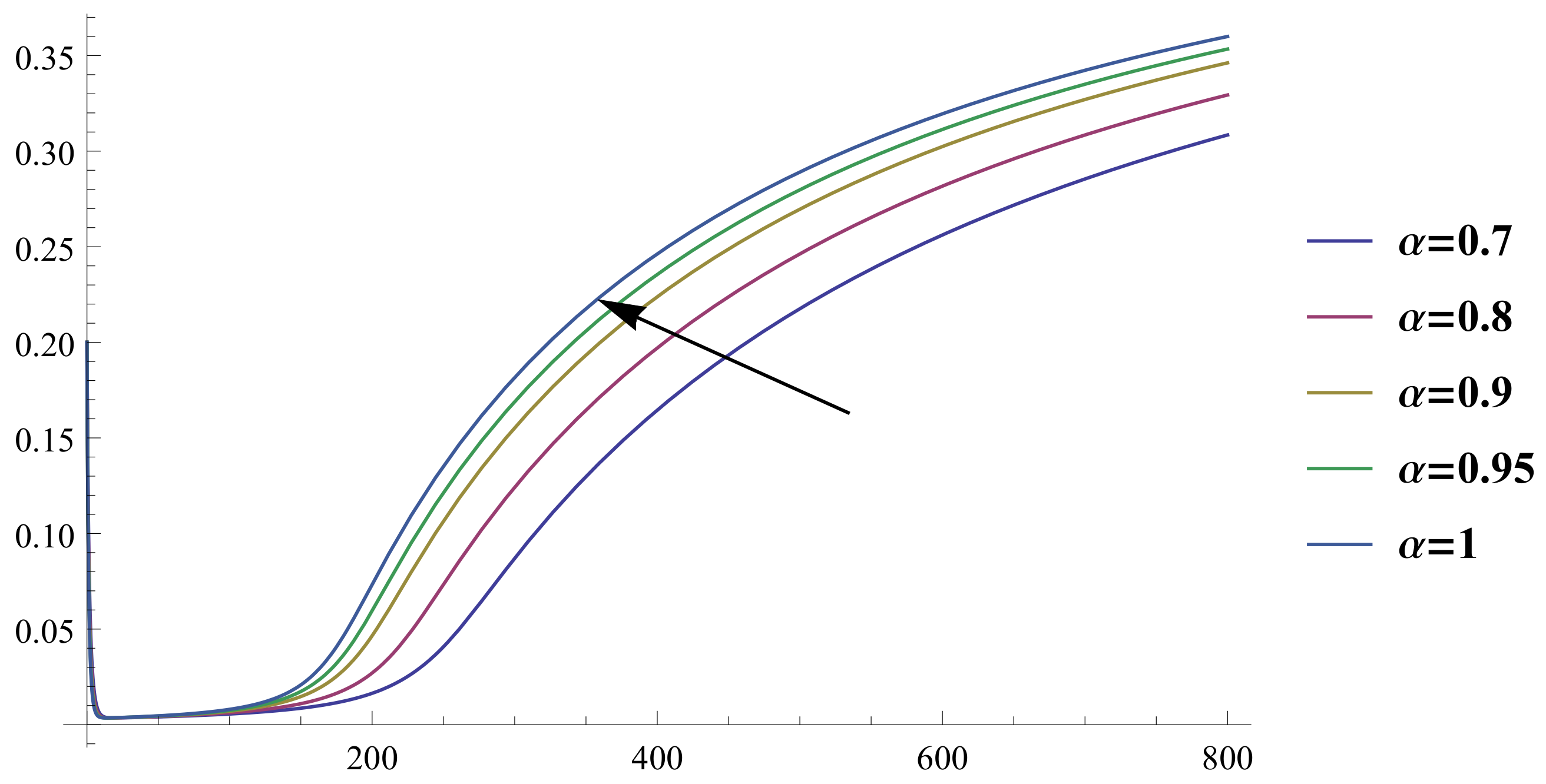
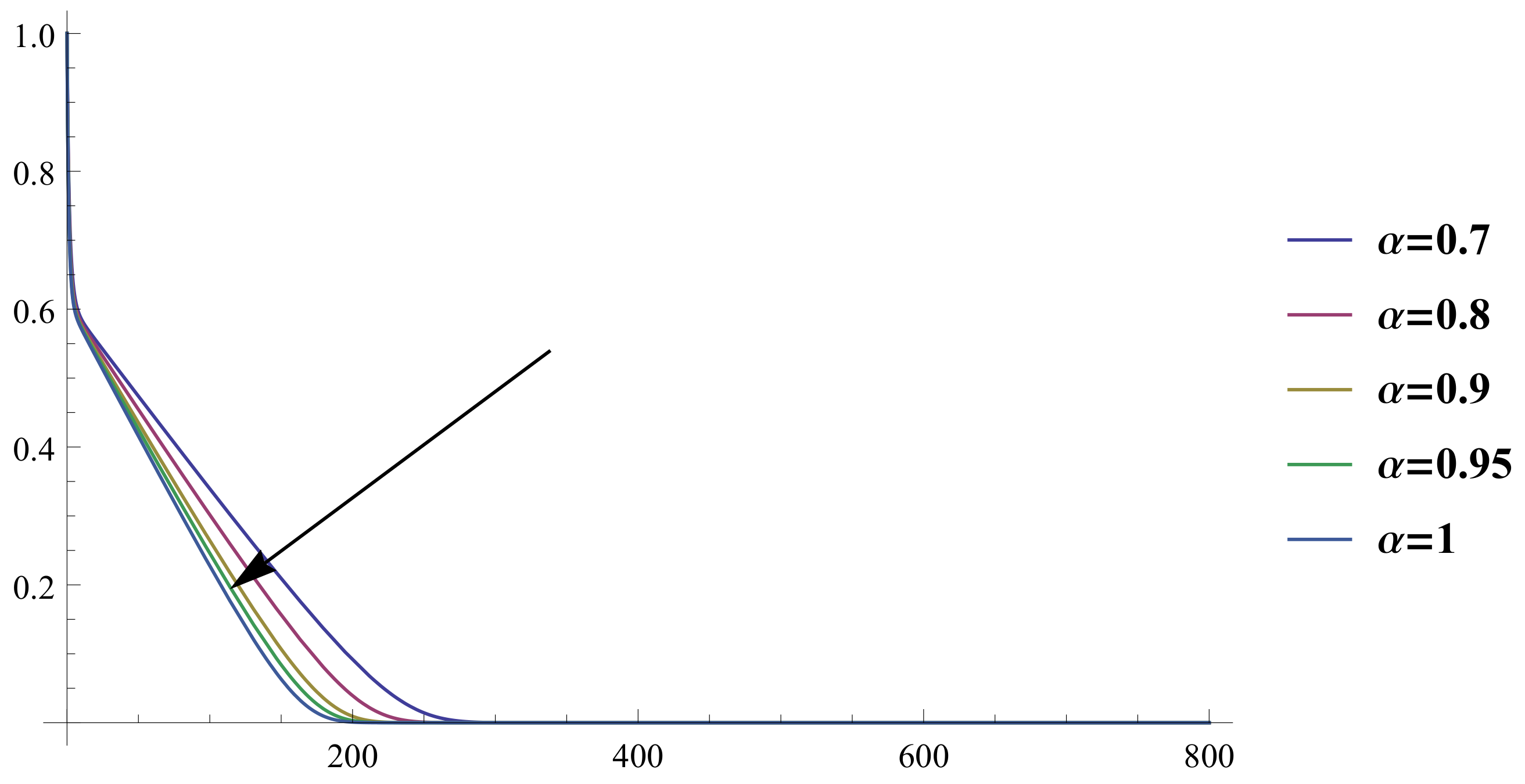
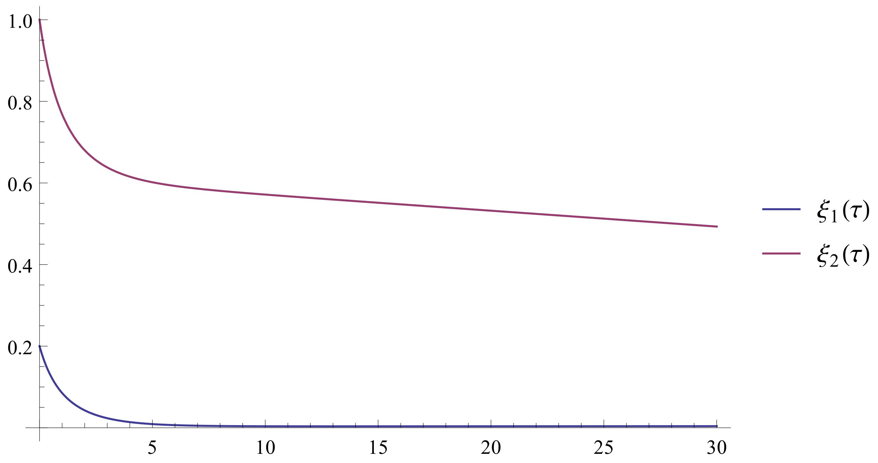
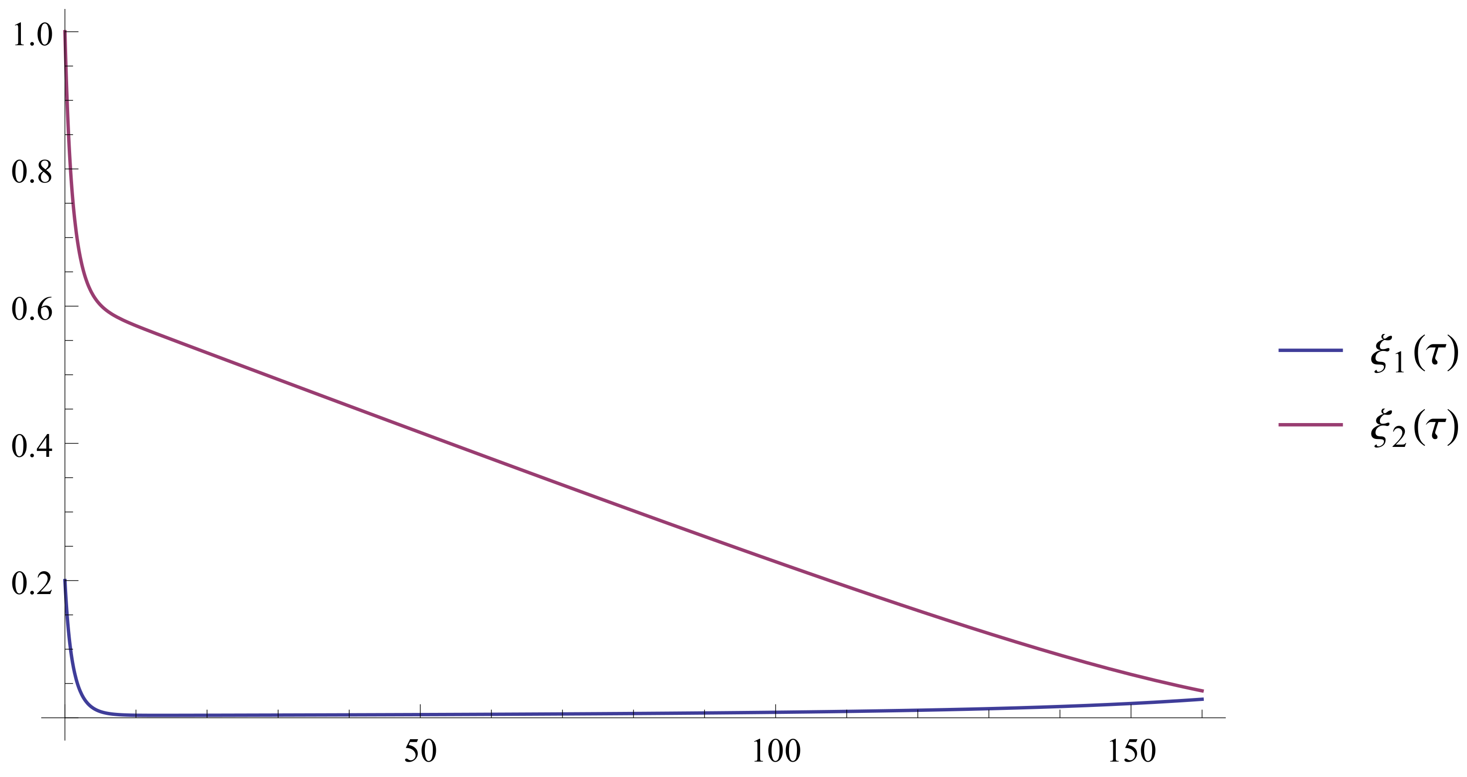
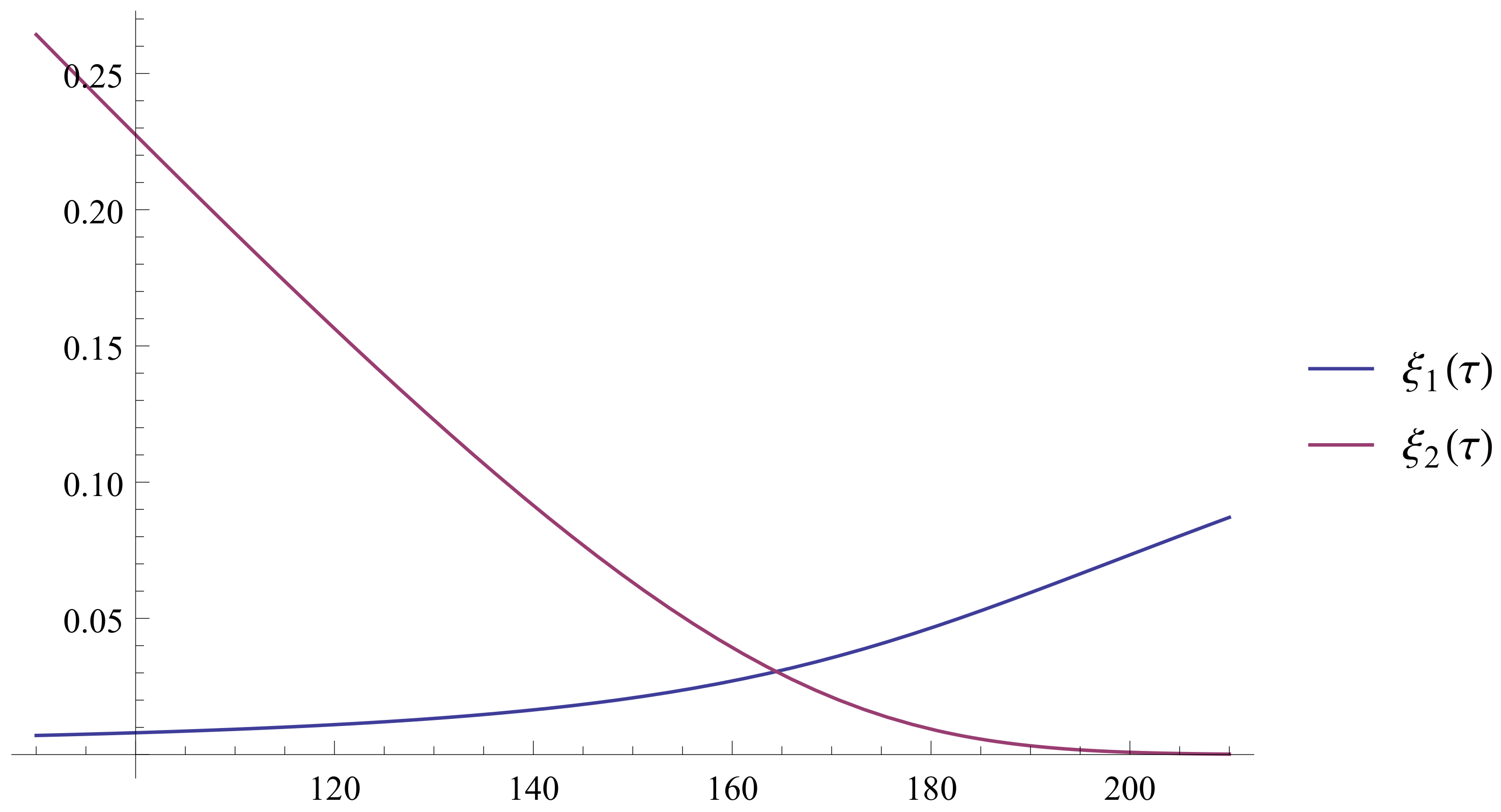
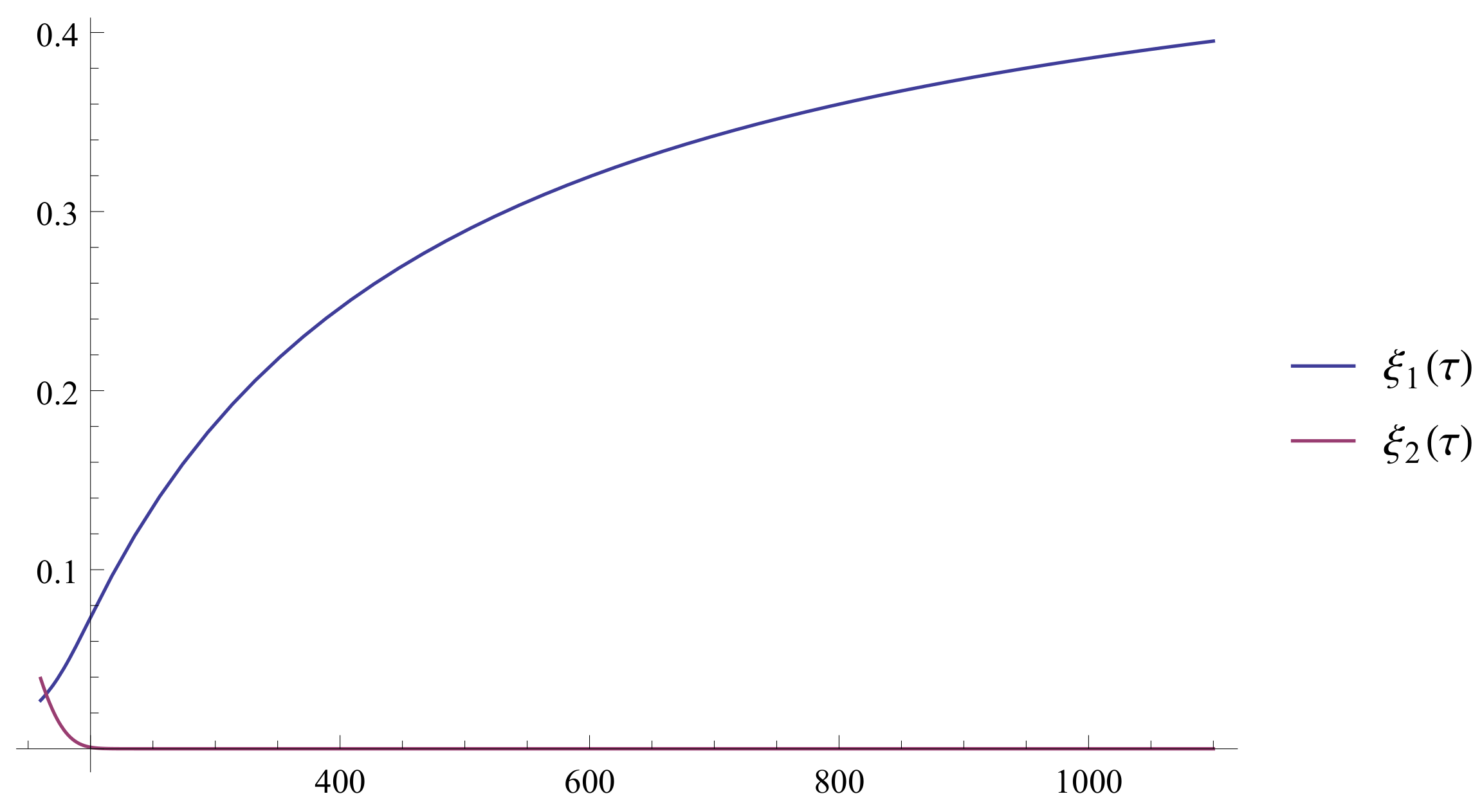
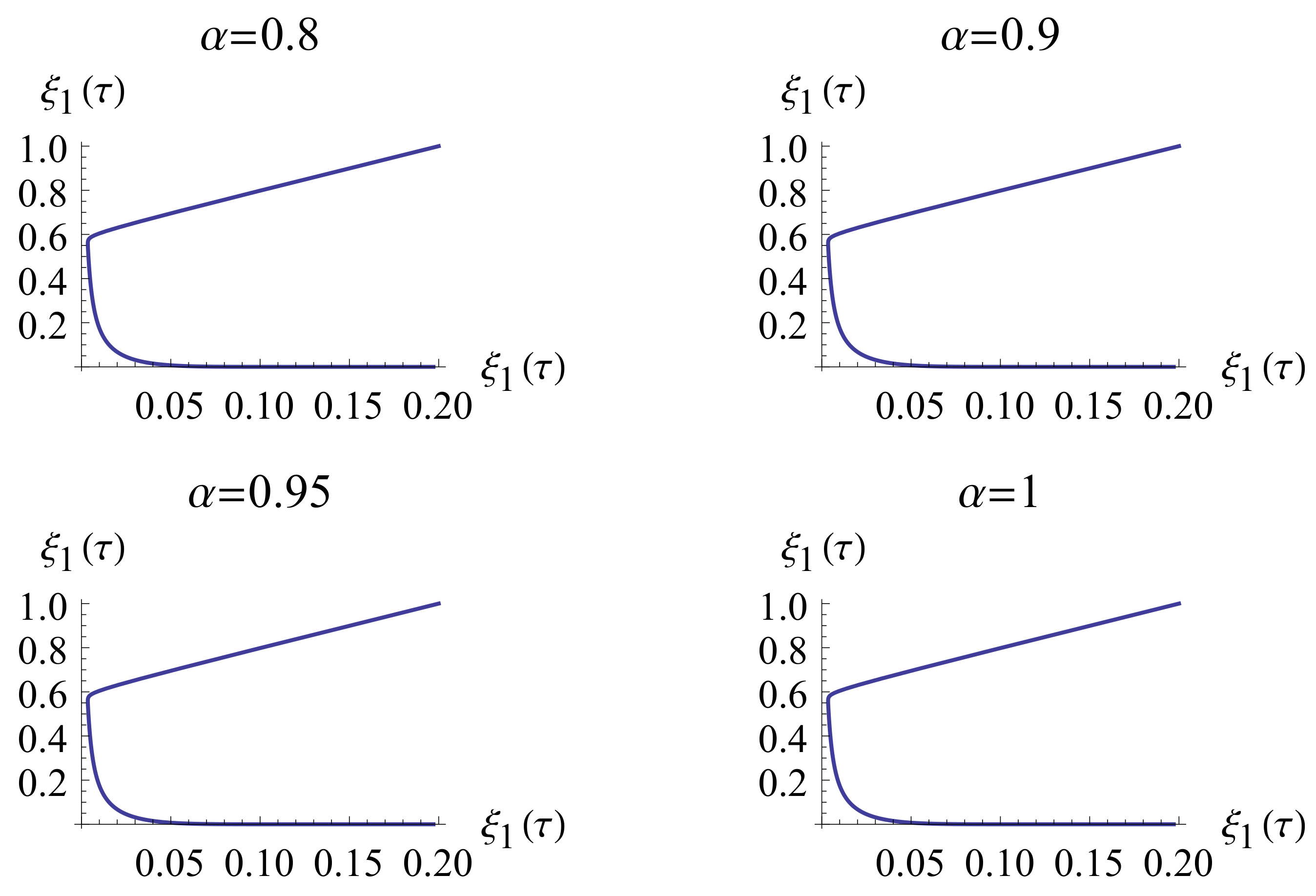
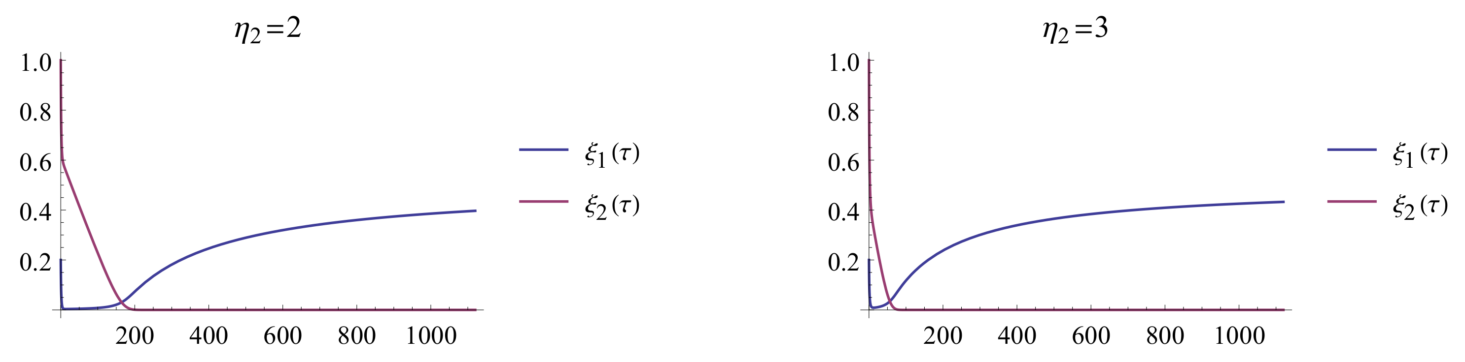
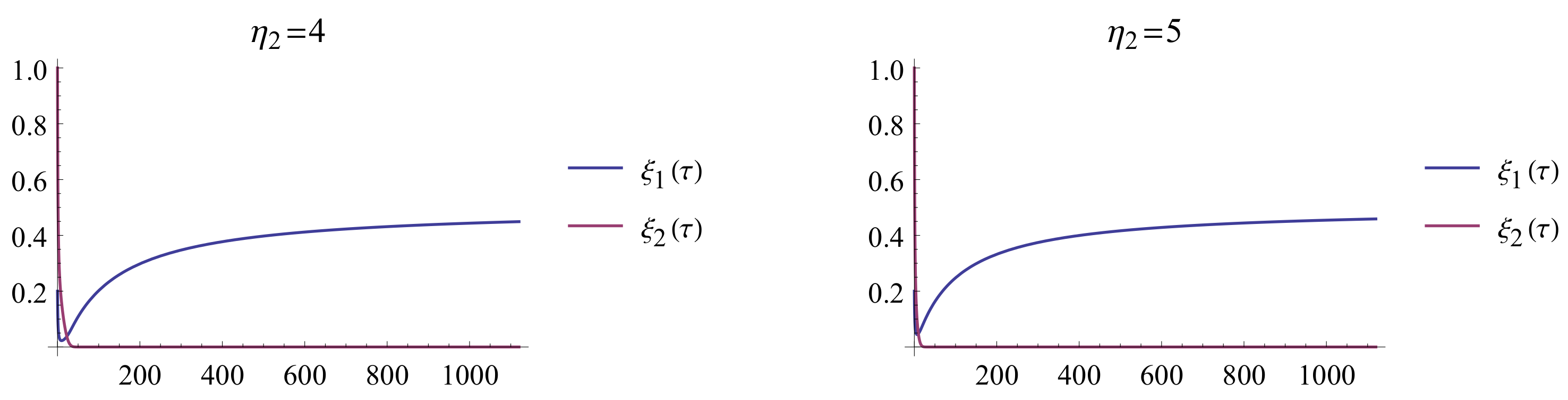
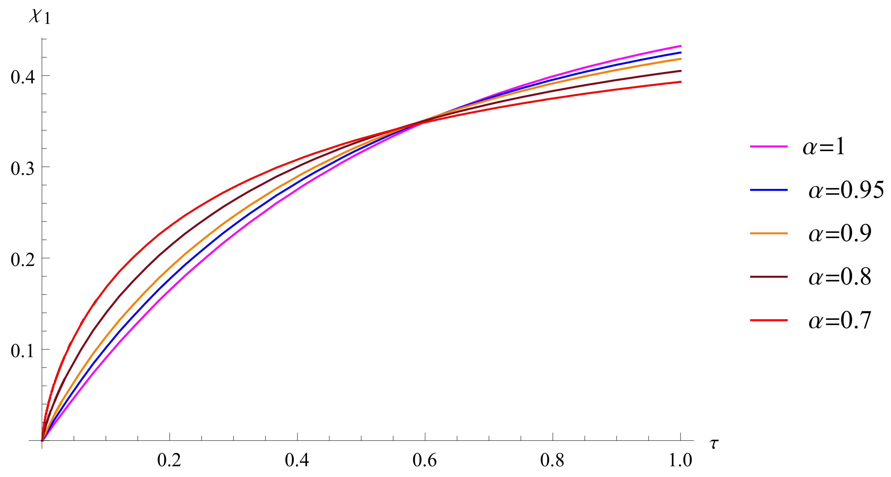
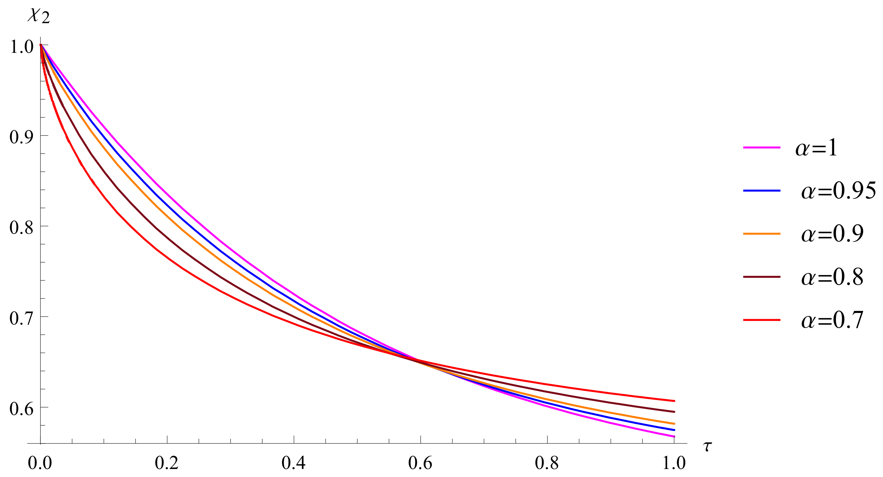
• Figure 3, Figure 4, Figure 5, Figure 6 and Figure 7 reveal that the behavior of concentrations ${\xi }_1$ and ${\xi }_2$ differs based on the value of $\tau$ when $\alpha =1$. The domain can be divided into four parts: rapid decay of ${\xi }_1$ and ${\xi }_2$ in the first interval, linear increase in ${\xi }_1$ and linear decay of ${\xi }_2$ in the second region, fast increase in ${\xi }_1$ and fast decay of ${\xi }_2$ in the third region, and linear increase in ${\xi }_1$ and rapid decay of ${\xi }_2$ in the fourth region. This behavior is consistent with [23].
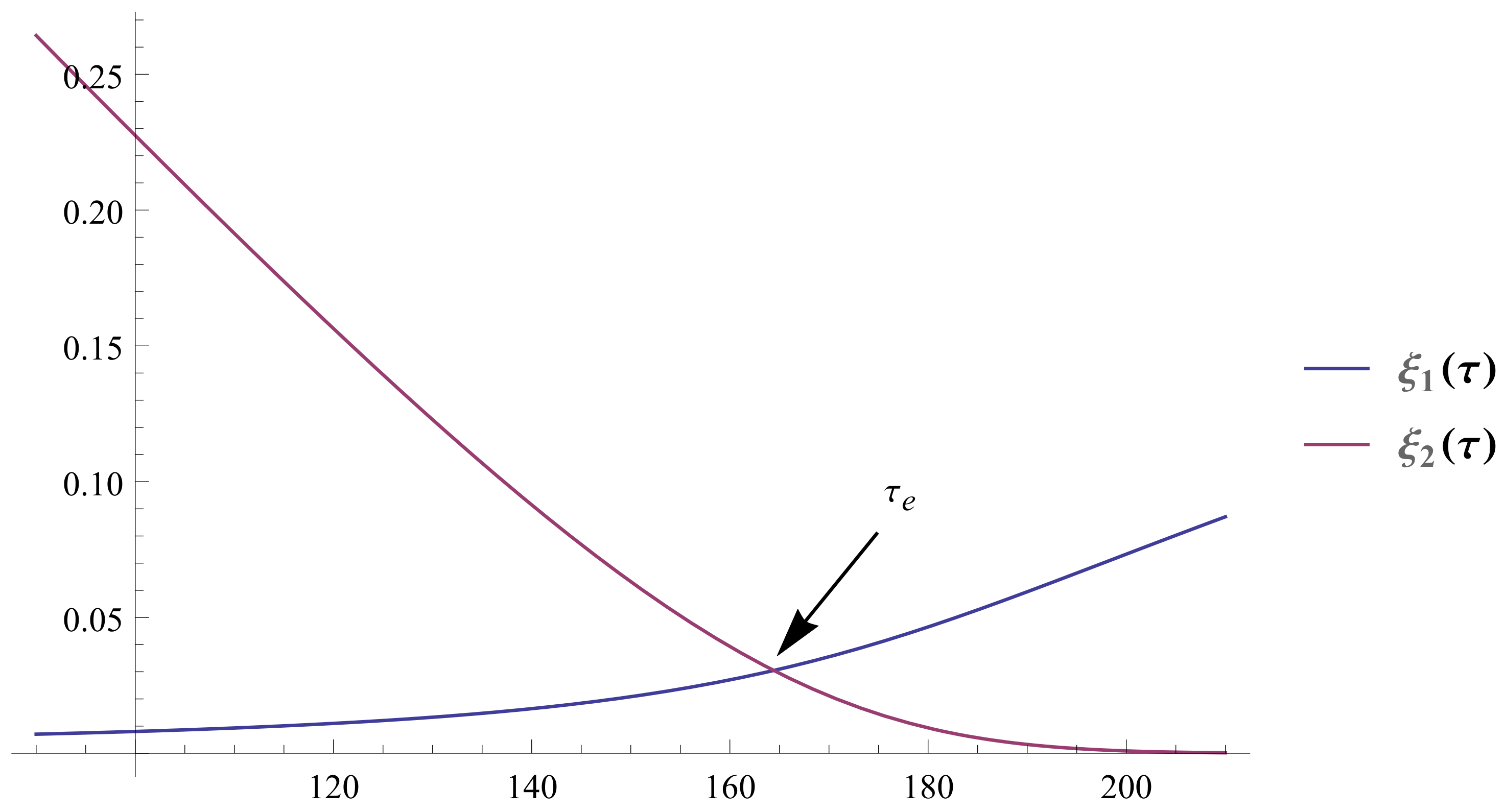
• Figure 5 visually indicates the end of the induction period ${\tau }_e$.
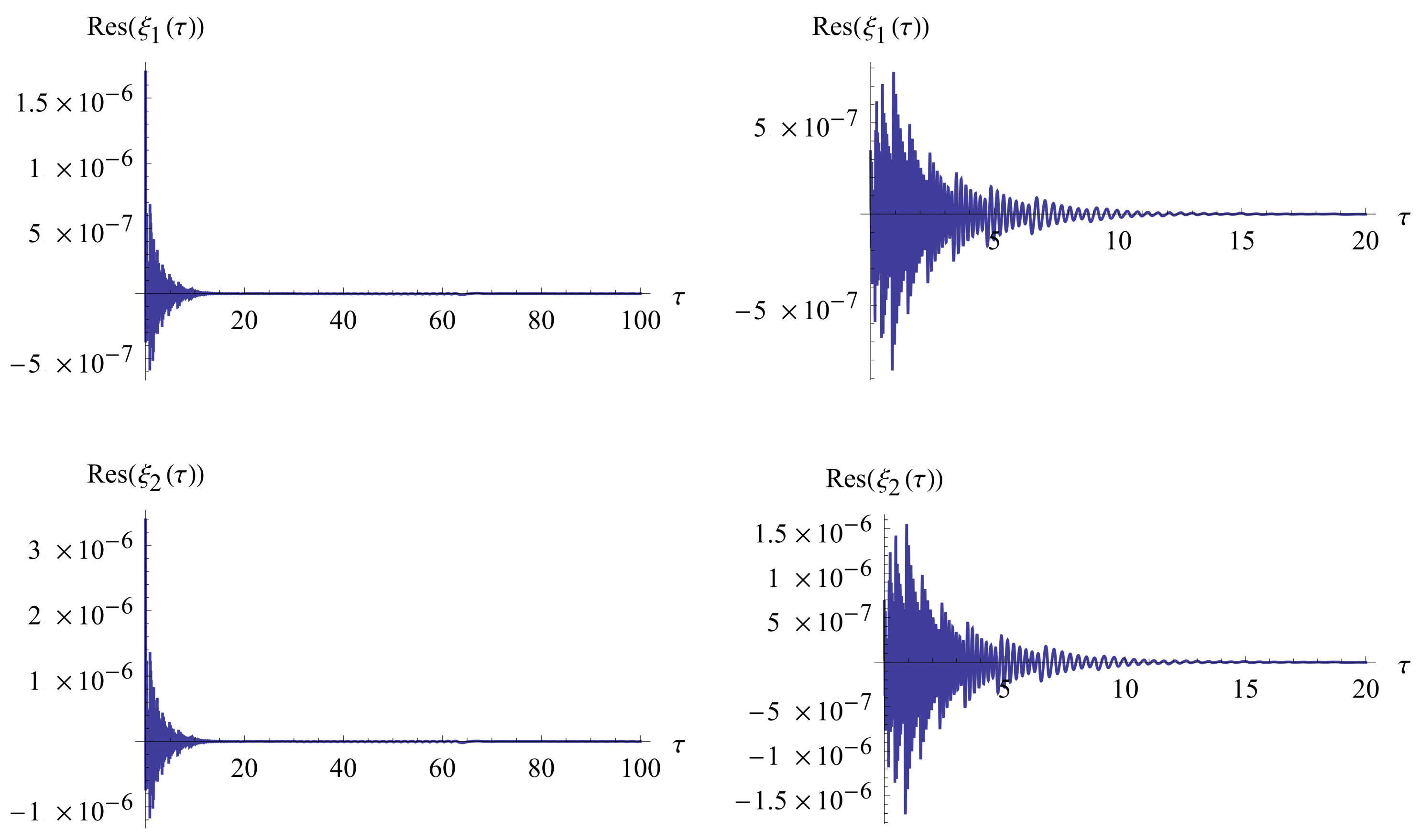
• Figure 8 shows that the residual errors of ${\xi }_1$ and ${\xi }_2$ are approximately ${10}^{-6}$, providing strong numerical evidence for the convergence of the proposed method.
• Figure 9 compares the behavior of the two approximate solutions and confirms their similarity to [23].
• Figure 10 and Figure 11 demonstrate the influence of ${\eta }_2$ on the approximate solutions. It affects the induction period when ${\xi }_1\left(\tau \right)={\xi }_2\left(\tau \right)$ but does not alter the shape of the solutions.
• Table 1 and Table 2 reveal that the induction period decreases as $\alpha$ increases and approaches one, with a similar effect when ${\eta }_2$ increases.
• As $\alpha$ approaches one, the approximate solutions converge to the solutions in [23].
• Figure 12 and Figure 13 illustrate the approximate solutions of ${\xi }_1$ and ${\xi }_2$ for the Riccati differential equations. The approximate solutions converge to the solutions obtained when $\alpha =1$, as the fractional order approaches one.
• Table 3 presents the maximum error for different values of $\alpha$, which is approximately ${10}^{-15}$. This indicates that the approximate solution converges to the exact solution.
• Table 4 compares the computation time in our approach with those in [29,31] for the optimal control problem. It is evident that our approach requires significantly less computational time compared to [29,31]. This demonstrates that our approach converges faster to the exact solution, which is attributed to reducing our algebraic system to a set of $2\times 2$ algebraic systems.
• Table 5 compares the absolute error in our approach with those in [29,31]. It is evident that the absolute error in our approach is smaller compared to [29,31]. This serves as strong numerical evidence that our approach converges faster to the exact solution.
• We can generalize our approach to boundary value problems using the linear shooting method. To do this, we assume initial conditions ${\theta }_1$ and ${\theta }_2$, and then we determine these values by solving the system using the given boundary conditions.

References

1. Amin, R.; Ahmad, H.; Shah, K.; Bilal Hafeez, M.; Sumelka, W. Theoretical and computational analysis of nonlinear fractional integro-differential equations via collocation method. Chaos Solitons Fractals 2021, 151, 111252. [Google Scholar] [CrossRef]
2. Biazar, J.; Sadri, K. Solution of weakly singular fractional integro-differential equations by using a new operational approach. J. Comput. Appl. Math. 2019, 352, 453–477. [Google Scholar] [CrossRef]
3. Sahu, P.; Saha Ray, S. Legendre spectral collocation method for the solution of the model describing biological species living together. J. Comput. Appl. Math. 2016, 296, 47–55. [Google Scholar] [CrossRef]
4. Roul, P.; Meyer, P. Numerical solutions of systems of nonlinear-differential equations by Homotopy-perturbation method. Appl. Math. Model. 2011, 35, 4234–4242. [Google Scholar] [CrossRef]
5. Shakeri, F.; Dehghan, M. Solution of a model describing biological species living together using the variational iteration method. Math. Comput. Model. 2008, 48, 685–699. [Google Scholar] [CrossRef]
6. Hatamzadeh-Varmazyar, S.; Masouri, Z.; Babolian, E. Numerical method for solving arbitrary linear differential equations using a set of orthogonal basis functions and operational matrix. Appl. Math. Model. 2016, 40, 233–253. [Google Scholar] [CrossRef]
7. Odibat, Z.M. Analytic study on linear systems of fractional differential equations. Comput. Math. Appl. 2010, 59, 1171–1183. [Google Scholar] [CrossRef] [Green Version]
8. Al-Refai, M. Fundamental results on systems of fractional differential equations in- volving Caputo-Fabrizio fractional derivative. Jordan J. Math. Stat. 2020, 13, 389–399. [Google Scholar]
9. Podlubny, I. Fractional Differential Equations; Academic Press: San Diego, CA, USA, 1999. [Google Scholar]
10. Syam, S.M.; Siri, Z.; Altoum, S.H.; Kasmani, R.M. Analytical and Numerical Methods for Solving Second-Order Two-Dimensional Symmetric Sequential Fractional Integro-Differential Equations. Symmetry 2023, 15, 1263. [Google Scholar] [CrossRef]
11. Katugampola, U.N. New approach to generalized fractional integral. Appl. Math. Comput. 2011, 218, 860–865. [Google Scholar] [CrossRef] [Green Version]
12. Baleanu, D.; Jaiami, A.; Sajjadi, S.; Mozyrski, D. A new fractional model and optimal control of a tumor-immune surveillance with non-singular derivative operator. Chaos 2019, 29, 083127. [Google Scholar] [CrossRef]
13. Caputo, M.; Fabrizio, M. A new definition of fractional derivative without singular kernel. Prog. Fract. Differ. Appl. 2015, 1, 73–85. [Google Scholar]
14. Atangana, A.; Baleanu, D. New fractional derivative with non-local and non-singular kernel. Therm. Sci. 2016, 20, 757–763. [Google Scholar] [CrossRef] [Green Version]
15. Da Vanterler, J.; Sousa, C.; Capelas de Oliveira, E. A Gronwall inequality and the Cauchy-type problem by means of Ψ-Hilfer operator. arXiv 2017, arXiv:1709.03634. [Google Scholar] [CrossRef] [Green Version]
16. Youbi, F.; Momani, S.; Hasan, S.; Al-Smadi, M. Effective numerical technique for nonlinear Caputo-Fabrizio Systems of fractional Volterra Integro-differential equations in Hilbert space. Alex. Eng. J. 2022, 61, 1778–1786. [Google Scholar] [CrossRef]
17. Zamanpour, I.; Ezzati, R. Operational matrix method for solving fractional weakly singular 2D partial Volterra integral equations. J. Comput. Appl. Math. 2023, 419, 114704. [Google Scholar] [CrossRef]
18. Syam, M.I.; Sharadga, M.; Hashim, I. A numerical method for solving fractional delay differential equations based on the operational matrix method. Chaos Solitons Fractals 2021, 147, 110977. [Google Scholar] [CrossRef]
19. Najafalizadeh, S.; Ezzati, R. A block pulse operational matrix method for solving two-dimensional nonlinear integro-differential equations of fractional order. J. Comput. Appl. Math. 2017, 326, 159–170. [Google Scholar] [CrossRef]
20. Richards, W.T.; Loomis, A.L. The chemical effects of high frequency sound waves I. A preliminary survey. J. Am. Chem. Soc. 1927, 49, 3086–3100. [Google Scholar] [CrossRef]
21. Forbes, G.S.; Estill, H.W.; Walker, O.J. Induction periods in reactions between thiosulfate and arsenite or arsenate: A useful clock reaction. J. Am. Chem. Soc. 1922, 44, 97–102. [Google Scholar] [CrossRef]
22. Horváth, A.K.; Nagypál, I. Classification of clock reactions. ChemPhysChem 2015, 16, 588–594. [Google Scholar] [CrossRef] [PubMed]
23. Kerr, R.; Thomson, W.M.; Smith, D.J. Mathematical modelling of the vitamin C clock reaction. R. Soc. Open Sci. 2019, 6, 181367. [Google Scholar] [CrossRef] [PubMed] [Green Version]
24. Wright, S.W. Tick tock, a vitamin C clock. J. Chem. Edu. 2002, 79, 40A. [Google Scholar] [CrossRef]
25. Wright, S.W. The vitamin C clock reaction. J. Chem. Edu. 2002, 79, 41. [Google Scholar] [CrossRef]
26. Rawlings, J.B.; Mayne, D.Q.; Diehl, M. Model Predictive Control: Theory and Design, 2nd ed.; Nob Hill Publishing: Santa Barbara, CA, USA, 2017. [Google Scholar]
27. Mehta, P.G. Principles of Control Systems Engineering; PHI Learning Pvt. Ltd: New Delhi, India, 2011. [Google Scholar]
28. Samko, S.G.; Kilbas, A.A.; Marichev, O.I. Fractional Integrals and Derivatives: Theory and Applications; Gordon and Breach: Yverdon, Switzerland, 1993. [Google Scholar]
29. Lotf, A.; Dehghan, M.; Yousef, S.A. A numerical technique for solving fractional optimal control problems. Comput. Math. Appl. 2011, 62, 1055–1067. [Google Scholar] [CrossRef] [Green Version]
30. Agrawal, O.P.; Baleanu, D. A Hamiltonian Formulation and a Direct Numerical Scheme for Fractional Optimal Control Problems. J. Vib. Control 2007, 13, 1269–1281. [Google Scholar] [CrossRef]
31. Keshavarz, E.; Ordokhani, Y.; Razzaghi, M. A numerical solution for fractional optimal control problems via Bernoulli polynomials. J. Vib. Control 2016, 22, 3889–3903. [Google Scholar] [CrossRef]
Figure 1. The approximate solution ξ 1 ( τ ) for α = 0.7 , 0.8 , 0.9 , 0.95 , 1 .
Mathematics 11 03132 g001
Figure 2. The approximate solution ξ 2 ( τ ) for α = 0.7 , 0.8 , 0.9 , 0.95 , 1 .
Mathematics 11 03132 g002
Figure 3. The approximate solutions ξ 1 ( τ ) and ξ 2 ( τ ) for α = 1 on [ 0 , 30 ] .
Mathematics 11 03132 g003
Figure 4. The approximate solutions ξ 1 ( τ ) and ξ 2 ( τ ) for α = 1 on [ 0 , 160 ] .
Mathematics 11 03132 g004
Figure 5. The approximate solutions ξ 1 ( τ ) and ξ 2 ( τ ) for α = 1 on [ 90 , 210 ] .
Mathematics 11 03132 g005
Figure 6. The approximate solutions ξ 1 ( τ ) and ξ 2 ( τ ) for α = 1 on [ 160 , 1100 ] .
Mathematics 11 03132 g006
Figure 7. The approximate solutions ξ 1 ( τ ) and ξ 2 ( τ ) for α = 1 on [ 0 , 1200 ] .
Mathematics 11 03132 g007
Figure 8. Residual errors of ξ 1 ( τ ) and ξ 2 ( τ ) for α = 1 .
Mathematics 11 03132 g008
Figure 9. The approximate solutions ξ 1 ( τ ) against each other.
Mathematics 11 03132 g009
Figure 10. The approximate solutions ξ 1 ( τ ) and ξ 2 ( τ ) for η 2 = 2 ,   3 .
Mathematics 11 03132 g010
Figure 11. The approximate solutions ξ 1 ( τ ) and ξ 2 ( τ ) for η 2 = 4 ,   5 .
Mathematics 11 03132 g011
Figure 12. The approximate solution ξ 1 ( τ ) for different values of α .
Mathematics 11 03132 g012
Figure 13. The approximate solution ξ 2 ( τ ) for different values of α .
Mathematics 11 03132 g013