


A Multi–Objective Gaining–Sharing Knowledge-Based Optimization Algorithm for Solving Engineering Problems
 , , ,
, , ,
Abstract
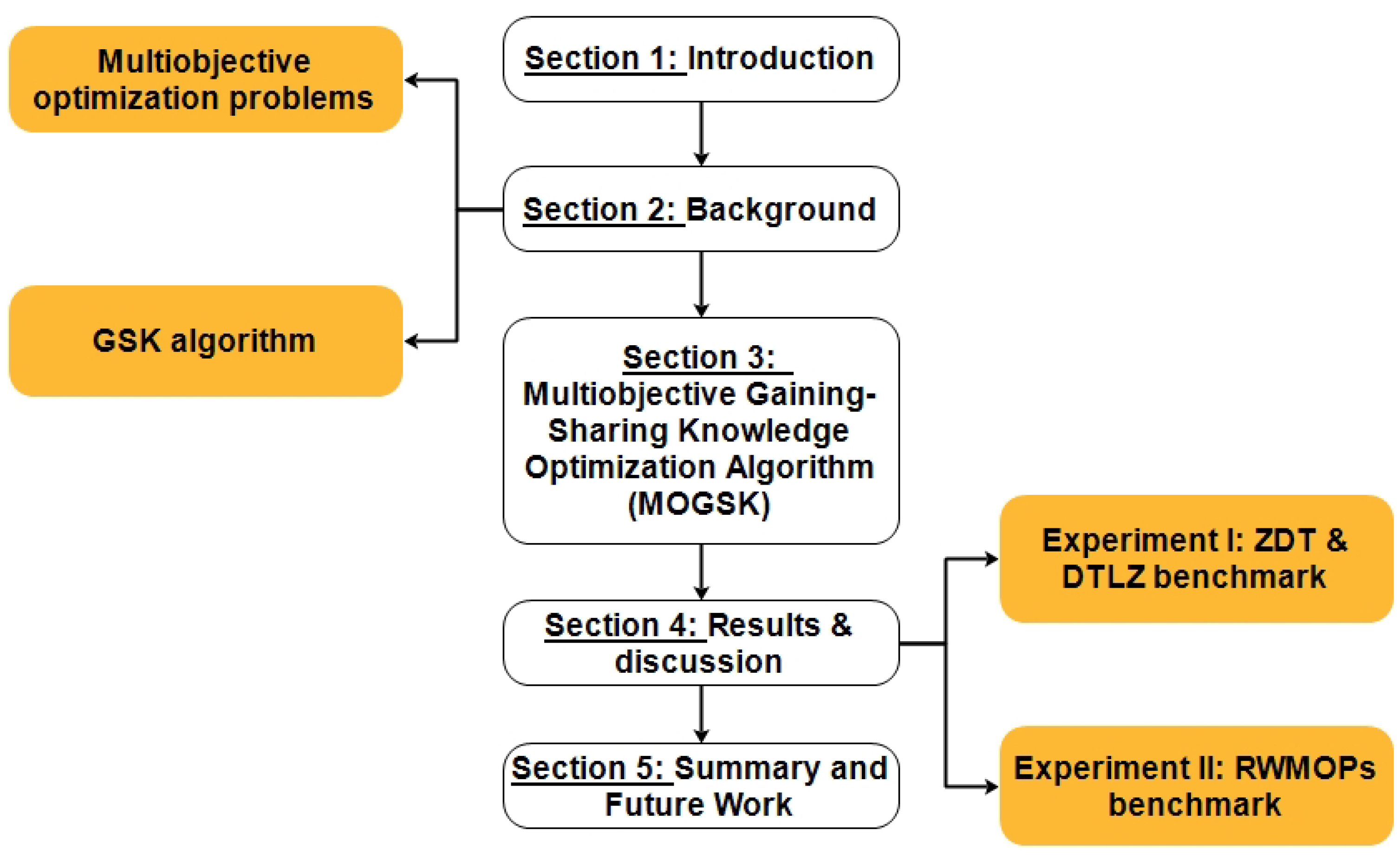
:1. Introduction
- We proposed an MOGSK to solve multiobjective optimization problems.
- The external archive was incorporated to maintain the nondominant solutions discovered so far and guide the particles toward the optimal Pareto set later in the exploration process.
- The -dominance relation was used to update the archive solutions. Additionally, it promoted exploitation and exploration while helping to increase diversity.
- In aim to preserve a good exploitation, diversity, and an effective solution distribution, the crowding distance and fast nondominated sorting were used.
- ZDT, DTLZ series test functions, and CEC 2021 RWMOPs (real-world constrained multiobjective optimization problems) were the test benchmarks to be utilized to validate the proposed MOGSK algorithm.
- In order to further evaluate the proposed MOGSK, a comparison was conducted against different algorithms, such as MOEAD, eMOEA, MOPSO, NSGAII, SPEA2, KnEA, and GrEA.
2. Background
2.1. Multiobjective Optimization Problems
2.2. Pareto Dominance
2.3. Gaining–Sharing Knowledge Optimization Algorithm (GSK)
- Junior gaining and sharing knowledge: in this stage, the individual tries to gain information from their small circle of people, such as family, relatives, and neighbors, since they cannot interact on a large scale such as social media. Even with a lack of experience, juniors still have the will to share their knowledge with the people they know or not; in addition, they do not have the ability yet to categorize people as bad or good, so they share due to curiosity and exploration.
- Senior gaining and sharing knowledge: in this stage, an individual is more experienced and has a wider circle of people to interact with, such as social networks, friends, and colleagues. Therefore, they gain their knowledge from their entourage. In addition, in this phase, they have an advanced ability to categorize people into classes such as best, better, and worst. Therefore, they share knowledge with the most suitable individuals and improve their skills.
- Initialization of the necessary factors, such as N—the population size, which corresponds to the number of people. Initialization of the starting population is random while respecting the boundary constraints, where represent the individuals; each corresponds to with , deferring to the possible number of fields of disciplines. To rephrase, it can be seen as branch of knowledge allocated to an individual. The fitness evaluation of the population noted as is also conducted.
- Now, the dimension between junior and senior is decided through the following nonlinear equation:and are the dimensions of junior and senior phases. k refers to the knowledge rate . G is the number of generations, while is the maximum number of generations.
- In this step, the junior gaining–sharing knowledge stage begins. In this stage each individual tries to gain knowledge from their small network; at the same time, they try to share their knowledge. The people that they interact with can be from their network or not, since in this phase, they are driven by curiosity.
- Now the update of the individuals in the current stage is conducted following the junior scheme:
- –
- Based on the values of the objective function, the individuals are sorted in ascendant order.
- –
- For each individual, the closest best and worst are selected to gain knowledge. In addition, a random individual is selected to share knowledge.
This step process is shown in Algorithm 1. is the knowledge factor, where ; this parameter controls the amount of knowledge (gained/shared) that is going to be added to the actual individual. is the knowledge ratio, where ; this parameter controls the amount of knowledge (gained/shared) that is going to be transferred to another individual.Algorithm 1 Phase 1: junior gaining and sharing knowledge [31]. ![Mathematics 11 03092 i001]()
- This step is the senior gaining–sharing knowledge phase. This stage takes into account a person’s capacity for classification (such as good and bad). And the scheme in this stage is as follows:
- –
- First, the values of the objective function are used to sort the individuals in ascendant order.
- –
- Then, those individuals are split into three groups: worst, middle, and best, for example: and .
- –
- Now, two vectors are chosen from the best and worst for gaining (100p%), while a third vector from the middle is chosen for sharing . p here indicates the percentage of best and worst individuals, where . This step process is shown in Algorithm 2.
Algorithm 2 Phase 2: senior gaining and sharing knowledge [31]. ![Mathematics 11 03092 i002]()


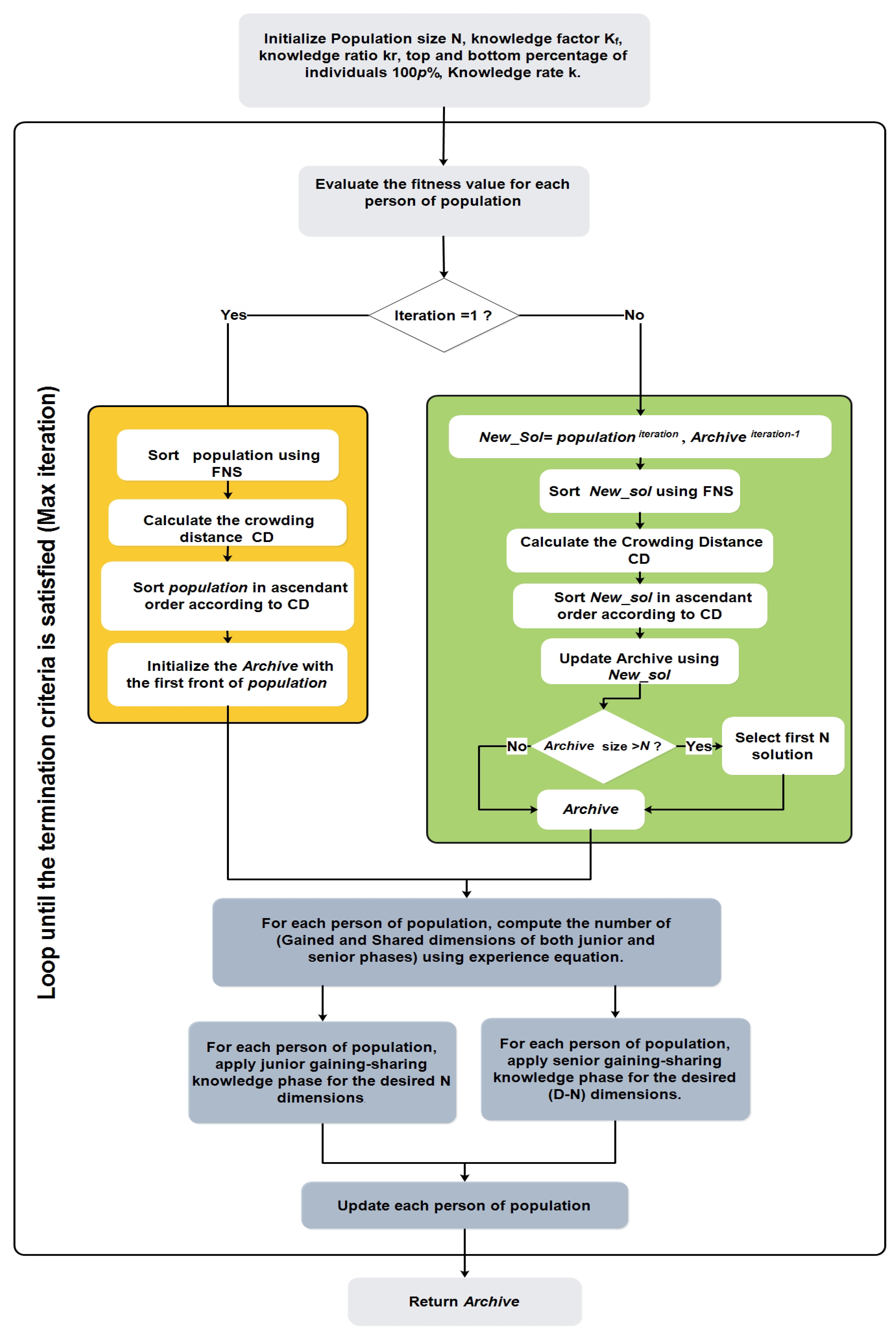
3. Multiobjective Gaining–Sharing Knowledge Optimization Algorithm (MOGSK)
- Fast nondominated sorting (FNS), in order to obtain the nondominated solutions.
- Crowding distance, to insure the distribution and convergence of the solutions as well as to improve the diversity.
- The archive, to preserve the best solutions so far and to act as a guide to the individual towards the Pareto optimal set.
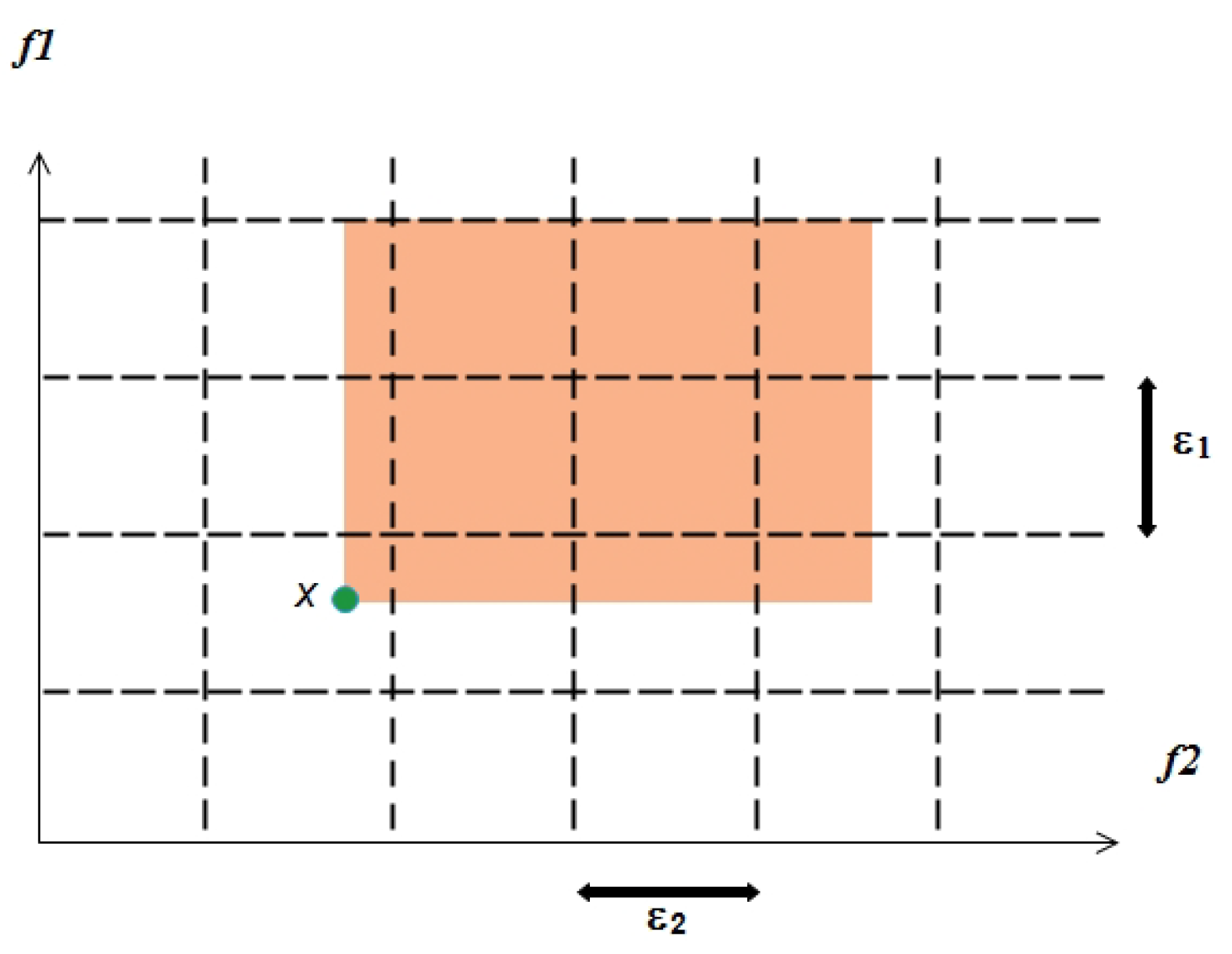
- The epsilon dominance relation, which is employed each iteration to update the archive’s solutions.
3.1. Update Population (Gaining/Sharing)
3.1.1. Solutions
3.1.2. Fast Nondominated Sorting (FNS)
3.1.3. Crowding Distance
3.2. Update Archive
-Dominance
| Algorithm 3 Updating archive solutions using -dominance. |
 |
| Algorithm 4 Multiobjective gaining–sharing knowledge optimization algorithm (MOGSK). |
 |
4. Results and Discussion
4.1. Experiments Setup
- Experiment I: ZDT, DTLZ test functions for MOPs.
- Experiment II: CEC 2021 test problems.
4.2. Experiment I
4.2.1. ZDT Test Results
4.2.2. DTLZ Test Results
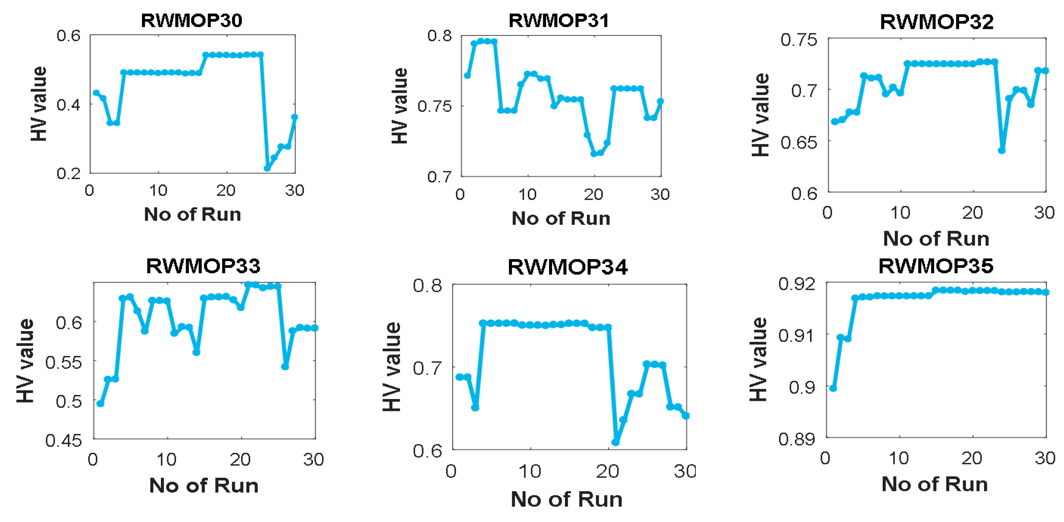
4.3. Experiment II
Limitation
5. Summary and Future Work
Author Contributions
Funding
Data Availability Statement
Acknowledgments
Conflicts of Interest
References
- Gunantara, N. A review of multi-objective optimization: Methods and its applications. Cogent Eng. 2018, 5, 1502242. [Google Scholar] [CrossRef]
- Mirjalili, S.; Jangir, P.; Saremi, S. Multi-objective ant lion optimizer: A multi-objective optimization algorithm for solving engineering problems. Appl. Intell. 2017, 46, 79–95. [Google Scholar] [CrossRef]
- Branke, J.; Deb, K.; Dierolf, H.; Osswald, M. Finding knees in multi-objective optimization. In Proceedings of the International Conference on Parallel Problem Solving from Nature, Birmingham, UK, 18–22 September 2004; pp. 722–731. [Google Scholar]
- Veldhuizen, D.; Lamont, G. Multiobjective evolutionary algorithms: Analyzing the state-of-the-art. Evol. Comput. 2000, 8, 125–147. [Google Scholar] [CrossRef] [PubMed]
- Kim, I.; Weck, O. Adaptive weighted-sum method for bi-objective optimization: Pareto front generation. Struct. Multidiscip. Optim. 2005, 29, 149–158. [Google Scholar] [CrossRef]
- Nedjah, N.; Mourelle, L.M. Evolutionary multi–objective optimisation: A survey. Int. J. Bio-Inspired Comput. 2015, 7, 1–25. [Google Scholar] [CrossRef]
- Holland, J. Adaptation in Natural and Artificial Systems: An Introductory Analysis with Applications to Biology, Control, and Artificial Intelligence. Available online: https://ieeexplore.ieee.org/book/6267401 (accessed on 15 June 2023).
- Srinivas, N.; Deb, K. Muiltiobjective optimization using nondominated sorting in genetic algorithms. Evol. Comput. 1994, 2, 221–248. [Google Scholar] [CrossRef]
- Deb, K.; Pratap, A.; Agarwal, S.; Meyarivan, T. A fast and elitist multiobjective genetic algorithm: NSGA-II. IEEE Trans. Evol. Comput. 2002, 6, 182–197. [Google Scholar] [CrossRef] [Green Version]
- Knowles, J.; Corne, D. M-PAES: A memetic algorithm for multiobjective optimization. Congr. Evol. Comput. 2000, 1, 325–332. [Google Scholar]
- Zhang, Q.; Li, H. MOEA/D: A multiobjective evolutionary algorithm based on decomposition. IEEE Trans. Evol. Comput. 2007, 11, 712–731. [Google Scholar] [CrossRef]
- Deb, K.; Mohan, M.; Mishra, S. Evaluating the ϵ-domination based multi-objective evolutionary algorithm for a quick computation of Pareto-optimal solutions. Evol. Comput. 2005, 13, 501–525. [Google Scholar] [CrossRef]
- Zitzler, E.; Laumanns, M.; Thiele, L. SPEA2: Improving the Strength Pareto Evolutionary Algorithm. Evol. Methods Des. Optim. Control. Appl. Ind. Probl. 2001, 103, 95–100. [Google Scholar] [CrossRef]
- Zhang, X.; Tian, Y.; Jin, Y. A knee point-driven evolutionary algorithm for many-objective optimization. IEEE Trans. Evol. Comput. 2014, 19, 761–776. [Google Scholar] [CrossRef]
- Yang, S.; Li, M.; Liu, X.; Zheng, J. A grid-based evolutionary algorithm for many-objective optimization. IEEE Trans. Evol. Comput. 2013, 17, 721–736. [Google Scholar] [CrossRef]
- Salcedo-Sanz, S.; Manjarres, D.; Pastor-Sánchez, Á.; Ser, J.; Portilla-Figueras, J.; Gil-Lopez, S. One-way urban traffic reconfiguration using a multi-objective harmony search approach. Expert Syst. Appl. 2013, 40, 3341–3350. [Google Scholar] [CrossRef]
- Sadollah, A.; Eskandar, H.; Bahreininejad, A.; Kim, J. Water cycle algorithm for solving multi-objective optimization problems. Soft Comput. 2015, 19, 2587–2603. [Google Scholar] [CrossRef]
- Zouache, D.; Moussaoui, A.; Abdelaziz, F. A cooperative swarm intelligence algorithm for multi-objective discrete optimization with application to the knapsack problem. Eur. J. Oper. Res. 2018, 264, 74–88. [Google Scholar] [CrossRef]
- Kumawat, I.; Nanda, S.; Maddila, R. Multi-objective whale optimization. In Proceedings of the Tencon 2017–2017 IEEE Region 10 Conference, Penang, Malaysia, 5–8 November 2017; pp. 2747–2752. [Google Scholar]
- Abdel-Basset, M.; Mohamed, R.; Mirjalili, S. A novel Whale Optimization Algorithm integrated with Nelder–Mead simplex for multi-objective optimization problems. Knowl.-Based Syst. 2021, 212, 106619. [Google Scholar] [CrossRef]
- Abdel-Basset, M.; Mohamed, R.; Mirjalili, S.; Chakrabortty, R.; Ryan, M. MOEO-EED: A multi-objective equilibrium optimizer with exploration–exploitation dominance strategy. Knowl.-Based Syst. 2021, 214, 106717. [Google Scholar] [CrossRef]
- Wang, Z.; Li, H.; Yu, H. MOEA/UE: A novel multi-objective evolutionary algorithm using a uniformly evolving scheme. Neurocomputing 2021, 458, 535–545. [Google Scholar] [CrossRef]
- Wang, W.; Tian, G.; Yuan, G.; Pham, D.T. Energy-time tradeoffs for remanufacturing system scheduling using an invasive weed optimization algorithm. J. Intell. Manuf. 2021, 34, 1065–1083. [Google Scholar] [CrossRef]
- Eberhart, R.; Kennedy, J. A new optimizer using particle swarm theory. In Proceedings of the MHS’95 Sixth International Symposium on Micro Machine and Human Science, Nagoya, Japan, 4–6 October 1995; pp. 39–43. [Google Scholar]
- Coello, C.; Pulido, G.; Lechuga, M. Handling multiple objectives with particle swarm optimization. IEEE Trans. Evol. Comput. 2004, 8, 256–279. [Google Scholar] [CrossRef]
- Dorigo, M.; Caro, G. Ant colony optimization: A new meta-heuristic. Congr. Evol. Comput. 1999, 2, 1470–1477. [Google Scholar]
- Alaya, I.; Solnon, C.; Ghedira, K. Ant colony optimization for multi-objective optimization problems. In Proceedings of the 19th IEEE International Conference on Tools with Artificial Intelligence (ICTAI 2007), Patras, Greece, 29–31 October 2007; Volume 1, pp. 450–457. [Google Scholar]
- Mirjalili, S. The ant lion optimizer. Adv. Eng. Softw. 2015, 83, 80–98. [Google Scholar] [CrossRef]
- Houssein, E.; Mahdy, M.; Shebl, D.; Manzoor, A.; Sarkar, R.; Mohamed, W. An efficient slime mould algorithm for solving multi-objective optimization problems. Expert Syst. Appl. 2022, 187, 115870. [Google Scholar] [CrossRef]
- Chalabi, N.; Attia, A.; Bouziane, A.; Hassaballah, M. An improved marine predator algorithm based on epsilon dominance and Pareto archive for multi-objective optimization. Eng. Appl. Artif. Intell. 2023, 119, 105718. [Google Scholar] [CrossRef]
- Mohamed, A.; Hadi, A.; Mohamed, A. Gaining-sharing knowledge based algorithm for solving optimization problems: A novel nature-inspired algorithm. Int. J. Mach. Learn. Cybern. 2020, 11, 1501–1529. [Google Scholar] [CrossRef]
- Reynolds, R.G. An introduction to cultural algorithms. In Evolutionary Programming—Proceedings of the Third Annual Conference; Sebald, A.V., Fogel, L.J., Eds.; World Scientific Press: San Diego, CA, USA, 1994; pp. 131–139. [Google Scholar]
- Geem, Z.W.; Kim, J.H.; Loganathan, G.V. A new heuristic optimization algorithm: Harmony search. Simulation 2001, 76, 60–68. [Google Scholar] [CrossRef]
- Kashan, A.H. League championship algorithm: A new algorithm for numerical function optimization. In Proceedings of the 2009 International Conference of Soft Computing and Pattern recognition, Malacca, Malaysia, 4–7 December 2009; pp. 43–48. [Google Scholar]
- Rao, R.V.; Savsani, V.J.; Vakharia, D. Teaching–learning-based optimization: A novel method for constrained mechanical design optimization problems. Comput.-Aided Des. 2011, 43, 303–315. [Google Scholar] [CrossRef]
- Shi, Y. Brain storm optimization algorithm. In Advances in Swarm Intelligence: Second International Conference, ICSI 2011, Chongqing, China, 12–15 June 2011, Proceedings, Part I 2; Springer: Berlin/Heidelberg, Germany, 2011; pp. 303–309. [Google Scholar]
- Kulkarni, A.J.; Durugkar, I.P.; Kumar, M. Cohort intelligence: A self supervised learning behavior. In Proceedings of the 2013 IEEE International Conference on Systems, Man, and Cybernetics, Manchester, UK, 13–16 October 2013; pp. 1396–1400. [Google Scholar]
- Moosavian, N.; Roodsari, B.K. Soccer league competition algorithm: A novel meta-heuristic algorithm for optimal design of water distribution networks. Swarm Evol. Comput. 2014, 17, 14–24. [Google Scholar] [CrossRef]
- Huan, T.T.; Kulkarni, A.J.; Kanesan, J.; Huang, C.J.; Abraham, A. Ideology algorithm: A socio-inspired optimization methodology. Neural Comput. Appl. 2017, 28, 845–876. [Google Scholar] [CrossRef]
- Moghdani, R.; Salimifard, K. Volleyball Premier League Algorithm. Appl. Soft Comput. J. 2018, 64, 161–185. [Google Scholar] [CrossRef]
- Khatri, A.; Gaba, A.; Rana, K.; Kumar, V. A novel life choice-based optimizer. Soft Comput. 2020, 24, 9121–9141. [Google Scholar] [CrossRef]
- Elsisi, M. Future search algorithm for optimization. Evol. Intell. 2019, 12, 21–31. [Google Scholar] [CrossRef]
- Shaheen, A.M.; Ginidi, A.R.; El-Sehiemy, R.A.; Ghoneim, S.S. A forensic-based investigation algorithm for parameter extraction of solar cell models. IEEE Access 2020, 9, 1–20. [Google Scholar] [CrossRef]
- Wagan, A.I.; Shaikh, M.M. A new metaheuristic optimization algorithm inspired by human dynasties with an application to the wind turbine micrositing problem. Appl. Soft Comput. 2020, 90, 106176. [Google Scholar]
- Emami, H. Anti-coronavirus optimization algorithm. Soft Comput. 2022, 26, 4991–5023. [Google Scholar] [CrossRef] [PubMed]
- Agrawal, P.; Ganesh, T.; Oliva, D.; Mohamed, A. S-shaped and V-shaped gaining-sharing knowledge-based algorithm for feature selection. Appl. Intell. 2022, 52, 81–112. [Google Scholar] [CrossRef]
- Xiong, G.; Yuan, X.; Mohamed, A.; Chen, J.; Zhang, J. Improved binary gaining-sharing knowledge-based algorithm with mutation for fault section location in distribution networks. J. Comput. Des. Eng. 2022, 9, 393–405. [Google Scholar] [CrossRef]
- Agrawal, P.; Ganesh, T.; Mohamed, A. Solving knapsack problems using a binary gaining sharing knowledge-based optimization algorithm. Complex Intell. Syst. 2022, 8, 43–63. [Google Scholar] [CrossRef]
- Li, C. Takagi–Sugeno fuzzy based power system fault section diagnosis models via genetic learning adaptive GSK algorithm. Knowl.-Based Syst. 2022, 255, 109773. [Google Scholar] [CrossRef]
- Ortega-Sánchez, N. Identification of apple diseases in digital images by using the Gaining-sharing knowledge-based algorithm for multilevel thresholding. Soft Comput. 2022, 26, 2587–2623. [Google Scholar] [CrossRef]
- Hassan, S.; Agrawal, P.; Ganesh, T.; Mohamed, A. A Novel Discrete Binary Gaining-Sharing Knowledge-Based Optimization Algorithm for the Travelling Counselling Problem for Utilization of Solar Energy. Int. J. Swarm Intell. Res. 2022, 13, 1–24. [Google Scholar] [CrossRef]
- Xiong, G.; Li, L.; Mohamed, A.; Yuan, X.; Zhang, J. A new method for parameter extraction of solar photovoltaic models using gaining–sharing knowledge based algorithm. Energy Rep. 2021, 7, 3286–3301. [Google Scholar] [CrossRef]
- Mohamed, A.; Hadi, A.; Mohamed, A.; Awad, N. Evaluating the Performance of Adaptive GainingSharing Knowledge Based Algorithm on CEC 2020 Benchmark Problems. In Proceedings of the 2020 IEEE Congress on Evolutionary Computation, CEC 2020, Glasgow, UK, 19–24 July 2020; pp. 1–8. [Google Scholar] [CrossRef]
- Mohamed, A.; Abutarboush, H.; Hadi, A.; Mohamed, A. Gaining-sharing knowledge based algorithm with adaptive parameters for engineering optimization. IEEE Access 2021, 9, 65934–65946. [Google Scholar] [CrossRef]
- Wolpert, D.; Macready, W. No free lunch theorems for optimization. IEEE Trans. Evol. Comput. 1997, 1, 67–82. [Google Scholar] [CrossRef] [Green Version]
- Rai, R.; Das, A.; Ray, S.; Dhal, K.G. Human-inspired optimization algorithms: Theoretical foundations, algorithms, open-research issues and application for multi-level thresholding. Arch. Comput. Methods Eng. 2022, 29, 5313–5352. [Google Scholar] [CrossRef]
- Zitzler, E.; Deb, K.; Thiele, L. Comparison of multiobjective evolutionary algorithms: Empirical results. Evol. Comput. 2000, 8, 173–195. [Google Scholar] [CrossRef] [Green Version]
- Deb, K.; Thiele, L.; Laumanns, M.; Zitzler, E. Scalable multi-objective optimization test problems. Congr. Evol. Comput. 2002, 1, 825–830. [Google Scholar]
- Kumar, A. A benchmark-suite of real-world constrained multi-objective optimization problems and some baseline results. Swarm Evol. Comput. 2021, 67, 100961. [Google Scholar] [CrossRef]
- Zitzler, E. Evolutionary algorithms for multiobjective optimization. Methods Appl. 1999, 63, 1–134. [Google Scholar]
- Tian, Y.; Cheng, R.; Zhang, X.; Jin, Y. PlatEMO: A MATLAB Platform for Evolutionary Multi-Objective Optimization[Educational Forum. IEEE Comput. Intell. Mag. 2017, 12, 73–87. [Google Scholar] [CrossRef] [Green Version]
- Kannan, B.; Kramer, S. An augmented lagrange multiplier based method for mixed integer discrete continuous optimization and its applications to mechanical design. In Proceedings of the ASME Design Engineering Technical Conference, Albuquerque, NM, USA, 19–22 September 1993; Volume Part F1679, pp. 103–112. [Google Scholar] [CrossRef]
- Narayanan, S.; Azarm, S. On improving multiobjective genetic algorithms for design optimization. Struct. Optim. 1999, 18, 146–155. [Google Scholar] [CrossRef]
- Chiandussi, G.; Codegone, M.; Ferrero, S.; Varesio, F. Comparison of multi-objective optimization methodologies for engineering applications. Comput. Math. Appl. 2012, 63, 912–942. [Google Scholar] [CrossRef] [Green Version]
- Deb, K. Evolutionary Algorithms for in Engineering Design. Evol. Algorithms Eng. Comput. Sci. 1999, 2, 135–161. [Google Scholar]
- Osyczka, A.; Kundu, S. A Genetic Algorithm-Based Multicriteria Optimization Method. In Proceedings of the First World Congress of Structural and Multidisciplinary Optimization, Goslar, Germany, 28 May–2 June 1995; pp. 909–914. [Google Scholar]
- Azarm, S.; Tits, A.; Fan, M. Tradeoff-driven optimization-based design of mechanical systems. In Proceedings of the 4th Symposium on Multidisciplinary Analysis and Optimization, Atlanta, GA, USA, 4–6 September 1999; p. 4758. [Google Scholar]
- Ray, T.; Liew, K. A swarm metaphor for multiobjective design optimization. Eng. Optim. 2002, 34, 141–153. [Google Scholar] [CrossRef]
- Deb, K.; Jain, H. An evolutionary many-objective optimization algorithm using reference-point-based nondominated sorting approach, Part I: Solving problems with box constraints. IEEE Trans. Evol. Comput. 2014, 18, 577–601. [Google Scholar] [CrossRef]
- Cheng, F.; Li, X. Generalized center method for multiobjective engineering optimization. Eng. Optim. 1999, 31, 641–661. [Google Scholar] [CrossRef]
- Huang, H.; Gu, Y.; Du, X. An interactive fuzzy multi-objective optimization method for engineering design. Eng. Appl. Artif. Intell. 2006, 19, 451–460. [Google Scholar] [CrossRef]
- Steven, G. Evolutionary Algorithms for Single and Multicriteria Design Optimization; Osyczka, A., Ed.; Springer: Berlin/Heidelberg, Germany, 2002; Volume 24. [Google Scholar]
- Coello, C.; Lamont, G.; Veldhuizen, D. Evolutionary Algorithms for Solving Multi-Objective Problems; Springer: Berlin/Heidelberg, Germany, 2007; Volume 5. [Google Scholar] [CrossRef]
- Parsons, M.; Scott, R. Formulation of Multicriterion Design Optimization Problems for Solution with Scalar Numerical Optimization Methods. J. Ship Res. 2004, 48, 61–76. [Google Scholar] [CrossRef]
- Fan, L.; Yoshino, T.; Xu, T.; Lin, Y.; Liu, H. A Novel Hybrid Algorithm for Solving Multiobjective Optimization Problems with Engineering Applications. Math. Probl. Eng. 2018, 2018, 5316379. [Google Scholar] [CrossRef] [Green Version]
- Dhiman, G.; Kumar, V. Multi-objective spotted hyena optimizer: A Multi-objective optimization algorithm for engineering problems. Knowl.-Based Syst. 2018, 150, 175–197. [Google Scholar] [CrossRef]
- Mahon, K.; Siddall, J. Optimal Engineering Design: Principles and Applications (Mechanical Engineering Series; CRC Press: Boca Raton, FL, USA, 1983; Volume 34. [Google Scholar] [CrossRef]
- Zhang, H.; Peng, Y.; Hou, L.; Tian, G.; Li, Z. A hybrid multi-objective optimization approach for energy-absorbing structures in train collisions. Inf. Sci. 2019, 481, 491–506. [Google Scholar] [CrossRef]
- Floudas, C. A Collection of Test Problems for Constrained Global Optimization Algorithms. Available online: https://www.amazon.com/Collection-Problems-Constrained-Optimization-Algorithms/dp/3540530320 (accessed on 5 May 2021).
- Ryoo, H.; Sahinidis, N. Global optimization of nonconvex NLPs and MINLPs with applications in process design. Comput. Chem. Eng. 1995, 19, 551–566. [Google Scholar] [CrossRef]
- Guillén-Gosálbez, G. A novel MILP-based objective reduction method for multi-objective optimization: Application to environmental problems. Comput. Chem. Eng. 2011, 35, 1469–1477. [Google Scholar] [CrossRef]
- Kocis, G.; Grossmann, I. A modelling and decomposition strategy for the minlp optimization of process flowsheets. Comput. Chem. Eng. 1989, 13, 797–819. [Google Scholar] [CrossRef]
- Kocis, G.; Grossmann, I. Global Optimization of Nonconvex Mixed-Integer Nonlinear Programming (Minlp) Problems in Process Synthesis. Ind. Eng. Chem. Res. 1988, 27, 1407–1421. [Google Scholar] [CrossRef]
- Floudas, C. Nonlinear and Mixed-Integer Optimization: Fundamentals and Applications; Oxford University Press: Oxford, UK, 1995. [Google Scholar]
- Rathore, A.; Holtz, J.; Boller, T. Synchronous optimal pulsewidth modulation for low-switching-frequency control of medium-voltage multilevel inverters. IEEE Trans. Ind. Electron. 2010, 57, 2374–2381. [Google Scholar] [CrossRef]
- Rathore, A.; Holtz, J.; Boller, T. Optimal pulsewidth modulation of multilevel inverters for low switching frequency control of medium voltage high power industrial AC drives. In Proceedings of the 2010 IEEE Energy Conversion Congress and Exposition, ECCE 2010, Atlanta, GA, USA, 12–16 September 2010. [Google Scholar] [CrossRef]
- Edpuganti, A.; Rathore, A. Fundamental Switching Frequency Optimal Pulsewidth Modulation of Medium-Voltage Cascaded Seven-Level Inverter. IEEE Trans. Ind. Appl. 2015, 51, 3485–3492. [Google Scholar] [CrossRef]
- Edpuganti, A.; Dwivedi, A.; Rathore, A.; Srivastava, R. Optimal pulsewidth modulation of cascade nine-level (9L) inverter for medium voltage high power industrial AC drives. In Proceedings of the IECON 2015—41st Annual Conference of the IEEE Industrial Electronics Society, Yokohama, Japan, 9–12 November 2015; pp. 4259–4264. [Google Scholar] [CrossRef]
- Edpuganti, A.; Rathore, A. Optimal pulsewidth modulation for common-mode voltage elimination scheme of medium-voltage modular multilevel converter-fed open-end stator winding induction motor drives. IEEE Trans. Ind. Electron. 2017, 64, 848–856. [Google Scholar] [CrossRef]
- Mishra, S.; Kumar, A.; Singh, D.; Misra, R. Butterfly Optimizer for Placement and Sizing of Distributed Generation for Feeder Phase Balancing. In Advances in Intelligent Systems and Computing; Springer: Berlin/Heidelberg, Germany, 2019; Volume 799, pp. 519–530. [Google Scholar] [CrossRef]
- Biswas, P.; Suganthan, P.; Mallipeddi, R.; Amaratunga, G. Multi-objective optimal power flow solutions using a constraint handling technique of evolutionary algorithms. Soft Comput. 2020, 24, 2999–3023. [Google Scholar] [CrossRef]
- Kumar, A.; Das, S.; Mallipeddi, R. An Inversion-Free Robust Power-Flow Algorithm for Microgrids. IEEE Trans. Smart Grid 2021, 12, 2844–2859. [Google Scholar] [CrossRef]
- Kumar, A.; Jha, B.; Das, S.; Mallipeddi, R. Power Flow Analysis of Islanded Microgrids: A Differential Evolution Approach. IEEE Access 2021, 9, 61721–61738. [Google Scholar] [CrossRef]
- Jha, B.; Kumar, A.; Dheer, D.; Singh, D.; Misra, R. A modified current injection load flow method under different load model of EV for distribution system. Int. Trans. Electr. Energy Syst. 2020, 30, 12284. [Google Scholar] [CrossRef]
- Kumar, A.; Jha, B.; Singh, D.; Misra, R. A New Current Injection Based Power Flow Formulation. Electr. Power Compon. Syst. 2020, 48, 268–280. [Google Scholar] [CrossRef]
- Kumar, A.; Jha, B.; Dheer, D.; Singh, D.; Misra, R. Nested backward/forward sweep algorithm for power flow analysis of droop regulated islanded microgrids. IET Gener. Transm. Distrib. 2019, 13, 3086–3095. [Google Scholar] [CrossRef]
- Kumar, A.; Jha, B.; Singh, D.; Misra, R. Current injection-based Newton–Raphson power-flow algorithm for droop-based islanded microgrids. IET Gener. Transm. Distrib. 2019, 13, 5271–5283. [Google Scholar] [CrossRef]
- Kumar, A.; Jha, B.; Dheer, D.; Misra, R.; Singh, D. A Nested-Iterative Newton-Raphson based Power Flow Formulation for Droop-based Islanded Microgrids. Electr. Power Syst. Res. 2020, 180, 106131. [Google Scholar] [CrossRef]
- Rivas-Dávalos, F.; Irving, M. An approach based on the strength pareto evolutionary algorithm 2 for power distribution system planning. In Lecture Notes in Computer Science; Springer: Berlin/Heidelberg, Germany, 2005; Volume 3410, pp. 707–720. [Google Scholar] [CrossRef]


| Algorithm Parameters | |
|---|---|
| N | Population size (number of individuals) = 100 |
| k | Knowledge rate = 10 |
| Knowledge ratio = 0.1 | |
| Knowledge factor = 0.9 | |
| Number of runs = 30 independent runs | |
| Maximum number of function evaluation = 60,000 | |
| Biobjective Test Functions | |
|---|---|
| Function | Description |
| ZDT1 | Has a convex front |
| ZDT2 | Nonconvex front |
| ZDT3 | Has a discontinuous front |
| ZDT4 | Has 221 local Pareto optimal fronts, as results highly multimodal |
| ZDT6 | Has a nonuniform search space |
| Three-Objective Test Functions | |
| Function | Description |
| DTLZ1 | Has a linear Pareto optimal front (POF) |
| DTLZ2 | Has a spherical POF |
| DTLZ3 | Has many POFs |
| DTLZ4 | The POF has a dense set of solutions to exist near the |
| DTLZ5 | This problem will verify the ability to converge to a degenerated curve. |
| DTLZ6 | 2M-1 disconnected Pareto optimal front. |
| DTLZ7 | Has a POF that combines straight line and a hyperplane. |
| Algorithm | MOGSK | MOEAD | eMOEA | MOPSO | NSGAII | SPEA2 | KnEA | GrEA |
|---|---|---|---|---|---|---|---|---|
| ZDT1 | ||||||||
| Best | 1.88E-04 | 4.16E-03 | 2.48E-02 | 3.50E-01 | 4.42E-03 | 3.81E-03 | 3.07E-02 | 6.34E-03 |
| Worst | 2.59E-04 | 6.27E-03 | 3.34E-02 | 1.25E+00 | 5.41E-03 | 4.15E-03 | 3.74E-01 | 1.36E-02 |
| Average | 2.13E-04 | 4.81E-03 | 2.92E-02 | 7.42E-01 | 4.76E-03 | 3.96E-03 | 1.77E-01 | 7.36E-03 |
| median | 2.12E-04 | 4.70E-03 | 2.94E-02 | 7.30E-01 | 4.71E-03 | 3.95E-03 | 1.67E-01 | 7.14E-03 |
| Std | 1.56E-05 | 4.67E-04 | 2.17E-03 | 2.23E-01 | 2.17E-04 | 7.50E-05 | 9.36E-02 | 1.29E-03 |
| ZDT2 | ||||||||
| Best | 1.83E-04 | 4.53E-03 | 2.68E-02 | 2.29E-02 | 4.55E-03 | 3.84E-03 | 5.87E-02 | 7.90E-03 |
| Worst | 1.24E-03 | 7.57E-03 | 3.73E-02 | 2.48E+00 | 5.34E-03 | 4.06E-03 | 1.26E-01 | 8.05E-03 |
| Average | 2.38E-04 | 5.42E-03 | 3.16E-02 | 1.68E+00 | 4.82E-03 | 3.94E-03 | 9.62E-02 | 8.00E-03 |
| median | 2.05E-04 | 5.22E-03 | 3.10E-02 | 1.77E+00 | 4.78E-03 | 3.94E-03 | 9.79E-02 | 8.01E-03 |
| Std | 1.89E-04 | 7.45E-04 | 3.15E-03 | 5.66E-01 | 1.82E-04 | 5.10E-05 | 1.83E-02 | 3.56E-05 |
| ZDT3 | ||||||||
| Best | 8.01E-03 | 1.22E-02 | 4.03E-02 | 2.19E-01 | 5.11E-03 | 4.70E-03 | 7.22E-03 | 1.15E-02 |
| Worst | 9.33E-03 | 4.31E-02 | 9.07E-02 | 1.00E+00 | 6.47E-03 | 5.07E-03 | 3.92E-02 | 1.60E-02 |
| Average | 8.97E-03 | 1.97E-02 | 6.62E-02 | 6.47E-01 | 5.47E-03 | 4.91E-03 | 1.09E-02 | 1.42E-02 |
| median | 9.06E-03 | 1.37E-02 | 6.50E-02 | 6.29E-01 | 5.41E-03 | 4.92E-03 | 1.00E-02 | 1.41E-02 |
| Std | 2.30E-04 | 1.14E-02 | 9.94E-03 | 1.95E-01 | 2.71E-04 | 8.91E-05 | 5.50E-03 | 1.17E-03 |
| ZDT4 | ||||||||
| Best | 6.57E-02 | 4.69E-03 | 2.62E-02 | 7.88E+00 | 4.39E-03 | 3.82E-03 | 1.32E-01 | 7.23E-02 |
| Worst | 2.53E-01 | 1.20E-02 | 3.62E-02 | 3.47E+01 | 4.93E-03 | 5.10E-03 | 3.74E-01 | 5.24E-01 |
| Average | 1.53E-01 | 7.76E-03 | 3.02E-02 | 1.57E+01 | 4.64E-03 | 4.06E-03 | 2.59E-01 | 3.11E-01 |
| median | 1.55E-01 | 7.20E-03 | 3.02E-02 | 1.55E+01 | 4.62E-03 | 3.94E-03 | 2.65E-01 | 3.08E-01 |
| Std | 5.57E-02 | 1.90E-03 | 2.28E-03 | 6.70E+00 | 1.53E-04 | 2.96E-04 | 5.94E-02 | 1.31E-01 |
| ZDT6 | ||||||||
| Best | 1.53E-04 | 3.36E-03 | 2.49E-02 | 5.20E-03 | 3.49E-03 | 3.05E-03 | 5.02E-03 | 5.67E-03 |
| Worst | 1.13E-03 | 5.81E-03 | 3.18E-02 | 5.51E+00 | 3.90E-03 | 3.14E-03 | 1.41E-02 | 6.18E-03 |
| Average | 2.60E-04 | 4.68E-03 | 2.90E-02 | 1.90E-01 | 3.68E-03 | 3.09E-03 | 7.22E-03 | 6.02E-03 |
| median | 1.82E-04 | 4.70E-03 | 2.93E-02 | 6.64E-03 | 3.65E-03 | 3.09E-03 | 6.41E-03 | 6.03E-03 |
| Std | 1.96E-04 | 5.93E-04 | 1.86E-03 | 1.00E+00 | 1.07E-04 | 2.22E-05 | 2.15E-03 | 1.29E-04 |
| Algorithm | MOGSK | MOEAD | eMOEA | MOPSO | NSGAII | SPEA2 | KnEA | GrEA |
|---|---|---|---|---|---|---|---|---|
| ZDT1 | ||||||||
| Best | 4.44E+00 | 7.19E-01 | 0.00E+00 | 3.22E-01 | 7.20E-01 | 7.20E-01 | 7.00E-01 | 7.17E-01 |
| Worst | 1.93E-01 | 7.17E-01 | 3.22E-01 | 0.00E+00 | 7.18E-01 | 7.20E-01 | 4.95E-01 | 7.09E-01 |
| Average | 5.56E-01 | 7.18E-01 | 8.75E-02 | 8.75E-02 | 7.19E-01 | 7.20E-01 | 6.16E-01 | 7.16E-01 |
| median | 2.55E-01 | 7.18E-01 | 5.92E-02 | 5.92E-02 | 7.19E-01 | 7.20E-01 | 6.24E-01 | 7.16E-01 |
| Std | 1.04E+00 | 5.85E-04 | 9.49E-02 | 9.49E-02 | 2.98E-04 | 1.28E-04 | 5.52E-02 | 1.45E-03 |
| ZDT2 | ||||||||
| Best | 4.61E+01 | 4.43E-01 | 0.00E+00 | 4.10E-01 | 4.44E-01 | 4.45E-01 | 3.90E-01 | 4.42E-01 |
| Worst | 2.60E-01 | 4.36E-01 | 4.10E-01 | 0.00E+00 | 4.44E-01 | 4.45E-01 | 3.31E-01 | 4.41E-01 |
| Average | 9.91E+00 | 4.41E-01 | 1.40E-02 | 1.40E-02 | 4.44E-01 | 4.45E-01 | 3.56E-01 | 4.41E-01 |
| median | 5.23E+00 | 4.42E-01 | 0.00E+00 | 0.00E+00 | 4.44E-01 | 4.45E-01 | 3.54E-01 | 4.41E-01 |
| Std | 1.00E+01 | 1.68E-03 | 7.49E-02 | 7.49E-02 | 2.07E-04 | 7.92E-05 | 1.59E-02 | 4.11E-05 |
| ZDT3 | ||||||||
| Best | 1.77E+00 | 6.89E-01 | 1.33E-02 | 4.77E-01 | 6.00E-01 | 6.00E-01 | 6.87E-01 | 5.98E-01 |
| Worst | 1.39E-01 | 5.83E-01 | 4.77E-01 | 1.33E-02 | 5.99E-01 | 5.99E-01 | 5.97E-01 | 5.96E-01 |
| Average | 2.38E-01 | 6.15E-01 | 1.60E-01 | 1.60E-01 | 5.99E-01 | 6.00E-01 | 6.01E-01 | 5.97E-01 |
| median | 1.76E-01 | 5.98E-01 | 1.44E-01 | 1.44E-01 | 5.99E-01 | 6.00E-01 | 5.98E-01 | 5.97E-01 |
| Std | 2.93E-01 | 3.58E-02 | 1.16E-01 | 1.16E-01 | 1.16E-04 | 5.90E-05 | 1.63E-02 | 4.36E-04 |
| ZDT4 | ||||||||
| Best | 7.46E-01 | 7.17E-01 | 0.00E+00 | 0.00E+00 | 7.20E-01 | 7.20E-01 | 6.43E-01 | 6.56E-01 |
| Worst | 5.34E-01 | 7.07E-01 | 0.00E+00 | 0.00E+00 | 7.18E-01 | 7.17E-01 | 4.93E-01 | 3.85E-01 |
| Average | 6.51E-01 | 7.12E-01 | 0.00E+00 | 0.00E+00 | 7.19E-01 | 7.20E-01 | 5.67E-01 | 5.29E-01 |
| median | 6.38E-01 | 7.13E-01 | 0.00E+00 | 0.00E+00 | 7.19E-01 | 7.20E-01 | 5.65E-01 | 5.34E-01 |
| Std | 4.80E-02 | 2.83E-03 | 0.00E+00 | 0.00E+00 | 4.36E-04 | 8.59E-04 | 3.64E-02 | 8.34E-02 |
| ZDT6 | ||||||||
| Best | 4.30E+00 | 3.88E-01 | 0.00E+00 | 3.86E-01 | 3.89E-01 | 3.89E-01 | 3.87E-01 | 3.86E-01 |
| Worst | 4.20E-01 | 3.84E-01 | 3.86E-01 | 0.00E+00 | 3.88E-01 | 3.89E-01 | 3.78E-01 | 3.86E-01 |
| Average | 2.89E+00 | 3.85E-01 | 3.69E-01 | 3.69E-01 | 3.88E-01 | 3.89E-01 | 3.85E-01 | 3.86E-01 |
| median | 3.26E+00 | 3.85E-01 | 3.82E-01 | 3.82E-01 | 3.88E-01 | 3.89E-01 | 3.86E-01 | 3.86E-01 |
| Std | 1.36E+00 | 1.01E-03 | 6.98E-02 | 6.98E-02 | 9.79E-05 | 2.52E-05 | 2.11E-03 | 1.33E-04 |
| Algorithm | MOGSK | MOEAD | eMOEA | MOPSO | NSGAII | SPEA2 | KnEA | GrEA |
|---|---|---|---|---|---|---|---|---|
| DTLZ1 | ||||||||
| Best | 8.77E-03 | 2.06E-02 | 3.39E-02 | 7.33E-01 | 2.57E-02 | 1.99E-02 | 2.37E-02 | 2.36E-02 |
| Worst | 4.82E-02 | 2.09E-02 | 4.24E-02 | 1.17E+01 | 2.99E-02 | 2.08E-02 | 1.44E-01 | 3.36E-01 |
| Average | 2.03E-02 | 2.06E-02 | 3.67E-02 | 5.96E+00 | 2.73E-02 | 2.02E-02 | 5.58E-02 | 8.59E-02 |
| median | 1.60E-02 | 2.06E-02 | 3.66E-02 | 5.82E+00 | 2.75E-02 | 2.02E-02 | 4.30E-02 | 7.19E-02 |
| Std | 1.09E-02 | 8.00E-05 | 1.52E-03 | 2.52E+00 | 9.78E-04 | 1.63E-04 | 3.18E-02 | 6.84E-02 |
| DTLZ2 | ||||||||
| Best | 1.00E-03 | 5.45E-02 | 6.07E-02 | 1.21E-01 | 6.48E-02 | 5.26E-02 | 6.31E-02 | 6.27E-02 |
| Worst | 1.16E-03 | 5.45E-02 | 6.72E-02 | 2.40E-01 | 7.46E-02 | 5.57E-02 | 7.43E-02 | 6.65E-02 |
| Average | 1.09E-03 | 5.45E-02 | 6.46E-02 | 1.69E-01 | 6.94E-02 | 5.43E-02 | 6.67E-02 | 6.39E-02 |
| median | 1.09E-03 | 5.45E-02 | 6.49E-02 | 1.67E-01 | 6.95E-02 | 5.42E-02 | 6.59E-02 | 6.38E-02 |
| Std | 4.00E-05 | 3.72E-07 | 1.42E-03 | 2.66E-02 | 2.03E-03 | 6.47E-04 | 2.88E-03 | 7.78E-04 |
| DTLZ3 | ||||||||
| Best | 2.77E-01 | 5.47E-02 | 6.87E-02 | 1.63E+00 | 6.45E-02 | 5.31E-02 | 6.60E-02 | 6.38E-02 |
| Worst | 6.31E-01 | 1.06E-01 | 8.22E-01 | 1.72E+02 | 7.68E-02 | 6.60E-02 | 2.03E-01 | 5.34E-01 |
| Average | 4.30E-01 | 6.22E-02 | 1.09E-01 | 6.74E+01 | 7.13E-02 | 5.60E-02 | 1.01E-01 | 1.17E-01 |
| median | 4.38E-01 | 5.92E-02 | 7.87E-02 | 5.93E+01 | 7.15E-02 | 5.49E-02 | 8.81E-02 | 6.80E-02 |
| Std | 9.42E-02 | 9.96E-03 | 1.36E-01 | 4.73E+01 | 3.17E-03 | 2.98E-03 | 3.34E-02 | 1.06E-01 |
| DTLZ4 | ||||||||
| Best | 2.36E-03 | 5.45E-02 | 6.51E-02 | 1.20E-01 | 6.35E-02 | 5.39E-02 | 6.06E-02 | 6.42E-02 |
| Worst | 5.44E-03 | 9.46E-01 | 5.53E-01 | 9.50E-01 | 7.12E-02 | 9.46E-01 | 9.46E-01 | 9.46E-01 |
| Average | 3.92E-03 | 2.57E-01 | 1.96E-01 | 3.14E-01 | 6.71E-02 | 2.46E-01 | 1.24E-01 | 2.36E-01 |
| median | 4.10E-03 | 5.45E-02 | 6.74E-02 | 2.71E-01 | 6.71E-02 | 5.51E-02 | 6.49E-02 | 6.73E-02 |
| Std | 8.39E-04 | 3.11E-01 | 2.18E-01 | 1.89E-01 | 2.02E-03 | 2.66E-01 | 2.23E-01 | 2.80E-01 |
| DTLZ5 | ||||||||
| Best | 8.80E-05 | 3.38E-02 | 5.30E-02 | 8.41E-03 | 5.30E-03 | 4.17E-03 | 7.61E-03 | 2.00E-02 |
| Worst | 2.04E-04 | 3.39E-02 | 7.20E-02 | 2.20E-02 | 7.20E-03 | 4.67E-03 | 1.41E-02 | 2.44E-02 |
| Average | 1.23E-04 | 3.39E-02 | 6.70E-02 | 1.21E-02 | 5.87E-03 | 4.41E-03 | 9.41E-03 | 2.15E-02 |
| median | 1.14E-04 | 3.39E-02 | 6.80E-02 | 1.16E-02 | 5.84E-03 | 4.41E-03 | 9.12E-03 | 2.13E-02 |
| Std | 2.73E-05 | 2.72E-05 | 4.55E-03 | 2.74E-03 | 3.79E-04 | 1.28E-04 | 1.32E-03 | 9.55E-04 |
| DTLZ6 | ||||||||
| Best | 2.24E-03 | 3.39E-02 | 5.85E-02 | 6.18E-01 | 5.48E-03 | 4.03E-03 | 4.38E-03 | 2.19E-02 |
| Worst | 3.38E-02 | 3.39E-02 | 6.59E-02 | 4.40E+00 | 6.78E-03 | 4.19E-03 | 5.95E-03 | 2.23E-02 |
| Average | 5.66E-03 | 3.39E-02 | 6.27E-02 | 2.48E+00 | 5.92E-03 | 4.09E-03 | 4.89E-03 | 2.23E-02 |
| median | 3.78E-03 | 3.39E-02 | 6.29E-02 | 2.27E+00 | 5.87E-03 | 4.09E-03 | 4.86E-03 | 2.23E-02 |
| Std | 6.09E-03 | 1.23E-05 | 1.86E-03 | 1.16E+00 | 2.74E-04 | 4.00E-05 | 3.41E-04 | 9.20E-05 |
| DTLZ7 | ||||||||
| Best | 8.53E-04 | 1.50E-01 | 5.76E-02 | 5.37E-01 | 7.00E-02 | 5.77E-02 | 5.79E-02 | 7.65E-02 |
| Worst | 1.30E-03 | 8.03E-01 | 8.14E-01 | 5.38E+00 | 8.76E-02 | 3.46E-01 | 3.52E-01 | 3.73E-01 |
| Average | 1.07E-03 | 1.77E-01 | 1.48E-01 | 2.85E+00 | 7.77E-02 | 7.90E-02 | 7.54E-02 | 9.36E-02 |
| median | 1.10E-03 | 1.55E-01 | 6.21E-02 | 2.81E+00 | 7.84E-02 | 6.01E-02 | 6.60E-02 | 8.42E-02 |
| Std | 1.11E-04 | 1.18E-01 | 1.77E-01 | 1.28E+00 | 4.38E-03 | 7.24E-02 | 5.23E-02 | 5.29E-02 |
| Algorithm | MOGSK | MOEAD | eMOEA | MOPSO | NSGAII | SPEA2 | KnEA | GrEA |
|---|---|---|---|---|---|---|---|---|
| DTLZ1 | ||||||||
| Best | 5.67E-01 | 8.42E-01 | 7.77E-01 | 0.00E+00 | 8.28E-01 | 8.43E-01 | 8.21E-01 | 8.13E-01 |
| Worst | 3.20E-01 | 8.38E-01 | 6.93E-01 | 0.00E+00 | 8.16E-01 | 8.38E-01 | 5.65E-01 | 2.41E-01 |
| Average | 4.76E-01 | 8.41E-01 | 7.27E-01 | 0.00E+00 | 8.23E-01 | 8.41E-01 | 7.39E-01 | 6.79E-01 |
| median | 4.97E-01 | 8.41E-01 | 7.27E-01 | 0.00E+00 | 8.23E-01 | 8.42E-01 | 7.54E-01 | 6.97E-01 |
| Std | 7.12E-02 | 7.62E-04 | 1.71E-02 | 0.00E+00 | 3.13E-03 | 1.25E-03 | 5.90E-02 | 1.27E-01 |
| DTLZ2 | ||||||||
| Best | 9.74E+00 | 5.60E-01 | 5.50E-01 | 4.12E-01 | 5.38E-01 | 5.57E-01 | 5.48E-01 | 5.60E-01 |
| Worst | 2.72E-01 | 5.60E-01 | 5.42E-01 | 2.85E-01 | 5.26E-01 | 5.53E-01 | 5.32E-01 | 5.57E-01 |
| Average | 1.12E+00 | 5.60E-01 | 5.46E-01 | 3.50E-01 | 5.32E-01 | 5.56E-01 | 5.44E-01 | 5.58E-01 |
| median | 3.24E-01 | 5.60E-01 | 5.46E-01 | 3.48E-01 | 5.33E-01 | 5.56E-01 | 5.45E-01 | 5.58E-01 |
| Std | 2.16E+00 | 5.63E-06 | 2.00E-03 | 3.13E-02 | 3.34E-03 | 1.10E-03 | 3.39E-03 | 7.19E-04 |
| DTLZ3 | ||||||||
| Best | 2.54E-01 | 5.56E-01 | 5.44E-01 | 0.00E+00 | 5.37E-01 | 5.61E-01 | 5.36E-01 | 5.58E-01 |
| Worst | 2.52E-01 | 4.52E-01 | 1.48E-03 | 0.00E+00 | 4.88E-01 | 5.15E-01 | 3.97E-01 | 3.24E-01 |
| Average | 2.54E-01 | 5.30E-01 | 4.90E-01 | 0.00E+00 | 5.20E-01 | 5.46E-01 | 5.00E-01 | 5.10E-01 |
| median | 2.54E-01 | 5.36E-01 | 5.07E-01 | 0.00E+00 | 5.22E-01 | 5.49E-01 | 5.13E-01 | 5.49E-01 |
| Std | 2.93E-04 | 2.19E-02 | 9.43E-02 | 0.00E+00 | 1.23E-02 | 1.03E-02 | 3.62E-02 | 7.46E-02 |
| DTLZ4 | ||||||||
| Best | 9.83E-01 | 5.60E-01 | 5.54E-01 | 4.81E-01 | 5.40E-01 | 5.57E-01 | 5.51E-01 | 5.60E-01 |
| Worst | 8.25E-01 | 9.09E-02 | 3.07E-01 | 8.36E-02 | 5.20E-01 | 9.09E-02 | 9.09E-02 | 9.09E-02 |
| Average | 9.31E-01 | 4.62E-01 | 4.86E-01 | 3.86E-01 | 5.34E-01 | 4.70E-01 | 5.15E-01 | 4.74E-01 |
| median | 9.42E-01 | 5.60E-01 | 5.49E-01 | 4.20E-01 | 5.35E-01 | 5.54E-01 | 5.45E-01 | 5.59E-01 |
| Std | 3.88E-02 | 1.56E-01 | 1.08E-01 | 1.05E-01 | 4.53E-03 | 1.22E-01 | 1.15E-01 | 1.42E-01 |
| DTLZ5 | ||||||||
| Best | 5.42E+04 | 1.82E-01 | 1.71E-01 | 1.95E-01 | 2.00E-01 | 2.00E-01 | 1.96E-01 | 1.89E-01 |
| Worst | 5.40E+03 | 1.82E-01 | 1.63E-01 | 1.74E-01 | 1.98E-01 | 1.99E-01 | 1.89E-01 | 1.88E-01 |
| Average | 2.07E+04 | 1.82E-01 | 1.69E-01 | 1.90E-01 | 1.99E-01 | 2.00E-01 | 1.94E-01 | 1.88E-01 |
| median | 1.46E+04 | 1.82E-01 | 1.69E-01 | 1.91E-01 | 1.99E-01 | 2.00E-01 | 1.94E-01 | 1.88E-01 |
| Std | 1.29E+04 | 1.49E-05 | 1.78E-03 | 4.54E-03 | 2.30E-04 | 1.76E-04 | 1.52E-03 | 3.50E-04 |
| DTLZ6 | ||||||||
| Best | 5.86E-01 | 1.82E-01 | 1.78E-01 | 0.00E+00 | 2.00E-01 | 2.00E-01 | 2.00E-01 | 1.88E-01 |
| Worst | 4.61E-01 | 1.82E-01 | 1.76E-01 | 0.00E+00 | 1.99E-01 | 2.00E-01 | 1.98E-01 | 1.88E-01 |
| Average | 5.19E-01 | 1.82E-01 | 1.77E-01 | 0.00E+00 | 1.99E-01 | 2.00E-01 | 2.00E-01 | 1.88E-01 |
| median | 5.21E-01 | 1.82E-01 | 1.77E-01 | 0.00E+00 | 1.99E-01 | 2.00E-01 | 2.00E-01 | 1.88E-01 |
| Std | 3.91E-02 | 6.44E-06 | 6.29E-04 | 0.00E+00 | 1.17E-04 | 4.09E-05 | 3.04E-04 | 1.68E-05 |
| DTLZ7 | ||||||||
| Best | 4.85E+03 | 2.58E-01 | 2.70E-01 | 1.86E-01 | 2.73E-01 | 2.78E-01 | 2.79E-01 | 2.75E-01 |
| Worst | 1.82E+02 | 2.02E-01 | 1.93E-01 | 0.00E+00 | 2.65E-01 | 2.43E-01 | 2.41E-01 | 2.31E-01 |
| Average | 1.80E+03 | 2.54E-01 | 2.56E-01 | 1.18E-02 | 2.68E-01 | 2.75E-01 | 2.76E-01 | 2.70E-01 |
| median | 1.87E+03 | 2.56E-01 | 2.65E-01 | 0.00E+00 | 2.68E-01 | 2.77E-01 | 2.78E-01 | 2.69E-01 |
| Std | 1.35E+03 | 9.85E-03 | 1.86E-02 | 4.05E-02 | 1.88E-03 | 8.51E-03 | 6.77E-03 | 7.95E-03 |
| Name | Problem |
|---|---|
| Mechanical Design Problems | |
| RWMOP1 | Design of Pressure Vessels [62] |
| RWMOP2 | Design of Vibrating Platform [63] |
| RWMOP3 | Design of Two-Bar Truss [64] |
| RWMOP4 | Design of Welded Beam [65] |
| RWMOP5 | Disc Brake Design [66] |
| RWMOP6 | Speed Reducer Design [67] |
| RWMOP7 | Gear Train Design [68] |
| RWMOP8 | Car Side Impact Design [69] |
| RWMOP9 | Four-Bar Plane Truss [70] |
| RWMOP10 | Two-Bar Plane Truss |
| RWMOP11 | Water Resource Management |
| RWMOP12 | Simply Supported I-beam Design [71] |
| RWMOP13 | Gear Box Design |
| RWMOP14 | Multiple-Disk Clutch Brake Design [72] |
| RWMOP15 | Spring Design [62] |
| RWMOP16 | Cantilever Beam Design [73] |
| RWMOP17 | Bulk Carrier Design [74] |
| RWMOP18 | Front Rail Design [75] |
| RWMOP19 | Multiproduct Batch Plant [76] |
| RWMOP20 | Hydrostatic Thrust Bearing Design [77] |
| RWMOP21 | Crash Energy Management for High-Speed Train Problem [78] |
| Chemical Engineering Problems | |
| RWMOP22 | Problem of Haverly’s Pooling Test [79] |
| RWMOP23 | Reactor Network Design [80] |
| RWMOP24 | Heat Exchanger Network Design [81] |
| Process, Design, and Synthesis Problems | |
| RWMOP25 | Process Synthesis Problem [82] |
| RWMOP26 | Process Synthesis, and Design Problem [83] |
| RWMOP27 | Process Flow Sheeting Problem [84] |
| RWMOP28 | Two-Reactor Problem [82] |
| RWMOP29 | Process Synthesis Problem [82] |
| Power Electronics Problems | |
| RWMOP30 | The problem of Synchronous Optimal Pulse-Width Modulation of 3-Level Inverters [85] |
| RWMOP31 | The problem of Synchronous Optimal Pulse-Width Modulation of 5-Level Inverters [86] |
| RWMOP32 | The problem of Synchronous Optimal Pulse-Width Modulation of 7-Level Inverters [87] |
| RWMOP33 | The problem of Synchronous Optimal Pulse-Width Modulation of 9-Level Inverters [88] |
| RWMOP34 | The problem of Synchronous Optimal Pulse-Width Modulation of 11-Level inverters [89] |
| RWMOP35 | Synchronous Optimal Pulse-Width Modulation of 13-Level Inverters [89] |
| Power System Optimization Problems | |
| RWMOP36 | The Problem of Optimal Sizing of Single-Phase Distribution Generation with Reactive Power Support for Phase Balancing at Main Transformer/Grid and Reducing Active Power Loss [90] |
| RWMOP37 | The Problem of Optimal Sizing of Single-Phase Distribution Generation with Reactive Power Support for Phase Balancing at Main Transformer/Grid and Reducing Reactive Power Loss [90] |
| RWMOP38 | The Problem of Optimal Sizing of Single-Phase Distribution Generation with Reactive Power Support for Reducing Active and Reactive Power Loss [90] |
| RWMOP39 | The Problem of Optimal Sizing of Single-Phase Distribution Generation with Reactive Power Support for Phase Balancing at Main Transformer/Grid and Reducing Active and Reactive Power Loss [90] |
| RWMOP40 | The Problem of Optimal Power Flow for Reducing Active and Reactive Power Loss [91] |
| RWMOP41 | The Problem of Optimal Power Flow for Reducing Voltage Deviation, Active and Reactive Power Loss [92] |
| RWMOP42 | The Problem of Optimal Power Flow for Reducing Voltage Deviation and Active Power Loss [93] |
| RWMOP43 | The Problem of Optimal Power Flow for Reducing Fuel Cost and Active Power Loss [94] |
| RWMOP44 | Optimal Power Flow for reducing Fuel Cost, Active and Reactive Power Loss [95] |
| RWMOP45 | Optimal Power Flow for Reducing Fuel Cost, Voltage Deviation, and Active Power Loss [91] |
| RWMOP46 | Optimal Power Flow for Minimizing Fuel Cost, Voltage Deviation, Active and Reactive Power Loss [91] |
| RWMOP47 | The Problem of Optimal Droop Setting for Reducing Active and Reactive Power Loss [96] |
| RWMOP48 | The Problem of Optimal Droop Setting for Reducing Voltage Deviation and Active Power Loss [97] |
| RWMOP49 | The Problem of Optimal Droop Setting for Reducing Voltage Deviation, Active and Reactive Power Loss [98] |
| RWMOP50 | Power Distribution System Planning [99] |
| Algorithm Problem | MOGSK | MOEAD | eMOEA | MOPSO | NSGAII | SPEA2 | KnEA | GrEA |
|---|---|---|---|---|---|---|---|---|
| RWMOP1 | ||||||||
| Best | 1.00E+00 | 9.89E-01 | 1.00E+00 | 9.97E-01 | 6.06E-01 | 9.99E-01 | 6.31E-01 | 9.89E-01 |
| Worst | 1.00E+00 | 9.89E-01 | 9.89E-01 | 9.89E-01 | 6.04E-01 | 9.89E-01 | 5.82E-01 | 9.89E-01 |
| Average | 1.00E+00 | 9.89E-01 | 9.95E-01 | 9.91E-01 | 6.05E-01 | 9.93E-01 | 5.93E-01 | 9.89E-01 |
| median | 1.00E+00 | 9.89E-01 | 9.95E-01 | 9.90E-01 | 6.05E-01 | 9.93E-01 | 5.90E-01 | 9.89E-01 |
| Std | 2.94E-06 | 1.13E-16 | 3.69E-03 | 2.54E-03 | 5.06E-04 | 3.49E-03 | 9.71E-03 | 1.13E-16 |
| RWMOP2 | ||||||||
| Best | 9.84E-01 | 1.00E+00 | 1.00E+00 | 1.00E+00 | 3.93E-01 | 1.00E+00 | 3.94E-01 | 1.00E+00 |
| Worst | 3.90E-01 | 1.00E+00 | 1.00E+00 | 1.00E+00 | 0.00E+00 | 1.00E+00 | 0.00E+00 | 1.00E+00 |
| Average | 6.96E-01 | 1.00E+00 | 1.00E+00 | 1.00E+00 | 2.70E-01 | 1.00E+00 | 2.62E-01 | 1.00E+00 |
| median | 6.48E-01 | 1.00E+00 | 1.00E+00 | 1.00E+00 | 3.03E-01 | 1.00E+00 | 2.74E-01 | 1.00E+00 |
| Std | 1.87E-01 | 0.00E+00 | 0.00E+00 | 0.00E+00 | 1.40E-01 | 1.00E+00 | 1.32E-01 | 0.00E+00 |
| RWMOP3 | ||||||||
| Best | 6.62E-01 | 0.00E+00 | 4.73E-01 | 0.00E+00 | 9.02E-01 | 3.42E-01 | 8.99E-01 | 6.03E-01 |
| Worst | 0.00E+00 | 0.00E+00 | 0.00E+00 | 0.00E+00 | 9.02E-01 | 0.00E+00 | 8.57E-01 | 0.00E+00 |
| Average | 1.10E-01 | 0.00E+00 | 1.58E-02 | 0.00E+00 | 9.02E-01 | 4.55E-02 | 8.87E-01 | 1.98E-01 |
| median | 0.00E+00 | 0.00E+00 | 0.00E+00 | 0.00E+00 | 9.02E-01 | 0.00E+00 | 8.89E-01 | 0.00E+00 |
| Std | 2.51E-01 | 0.00E+00 | 8.64E-02 | 0.00E+00 | 1.55E-04 | 8.43E-02 | 9.96E-03 | 2.69E-01 |
| RWMOP4 | ||||||||
| Best | 8.74E-01 | 0.00E+00 | 0.00E+00 | 7.90E-01 | 8.63E-01 | 1.54E-01 | 7.93E-01 | 6.32E-01 |
| Worst | 8.69E-01 | 0.00E+00 | 0.00E+00 | 0.00E+00 | 8.57E-01 | 0.00E+00 | 6.89E-01 | 0.00E+00 |
| Average | 8.72E-01 | 0.00E+00 | 0.00E+00 | 3.67E-01 | 8.61E-01 | 5.15E-03 | 7.37E-01 | 2.11E-02 |
| median | 8.72E-01 | 0.00E+00 | 0.00E+00 | 4.20E-01 | 8.62E-01 | 0.00E+00 | 7.36E-01 | 0.00E+00 |
| Std | 1.14E-03 | 0.00E+00 | 0.00E+00 | 2.98E-01 | 1.59E-03 | 2.82E-02 | 2.34E-02 | 1.15E-01 |
| RWMOP5 | ||||||||
| Best | 6.30E-01 | 5.77E-01 | 2.51E-01 | 2.76E-01 | 4.35E-01 | 2.77E-01 | 4.14E-01 | 2.77E-01 |
| Worst | 6.29E-01 | 5.77E-01 | 2.48E-01 | 2.56E-01 | 4.27E-01 | 2.67E-01 | 3.18E-01 | 2.61E-01 |
| Average | 6.30E-01 | 5.77E-01 | 2.49E-01 | 2.67E-01 | 4.33E-01 | 2.73E-01 | 3.96E-01 | 2.74E-01 |
| median | 6.30E-01 | 5.77E-01 | 2.50E-01 | 2.68E-01 | 4.34E-01 | 2.73E-01 | 4.02E-01 | 2.74E-01 |
| Std | 1.27E-04 | 2.59E-08 | 7.58E-04 | 6.32E-03 | 1.75E-03 | 2.60E-03 | 2.20E-02 | 2.70E-03 |
| RWMOP6 | ||||||||
| Best | 3.20E-01 | 6.87E-02 | 3.07E-01 | 3.07E-01 | 2.77E-01 | 3.00E-01 | 2.72E-01 | 2.45E-01 |
| Worst | 3.19E-01 | 6.87E-02 | 1.11E-01 | 0.00E+00 | 2.77E-01 | 0.00E+00 | 1.84E-01 | 1.99E-02 |
| Average | 3.19E-01 | 6.87E-02 | 2.17E-01 | 1.15E-01 | 2.77E-01 | 1.69E-01 | 2.16E-01 | 1.47E-01 |
| median | 3.19E-01 | 6.87E-02 | 2.26E-01 | 9.27E-02 | 2.77E-01 | 1.53E-01 | 2.02E-01 | 1.53E-01 |
| Std | 5.63E-05 | 1.34E-05 | 5.89E-02 | 1.04E-01 | 3.27E-05 | 9.98E-02 | 2.90E-02 | 5.54E-02 |
| RWMOP7 | ||||||||
| Best | 4.83E-01 | 4.81E-01 | 4.84E-01 | 4.82E-01 | 4.84E-01 | 4.83E-01 | 4.84E-01 | 4.82E-01 |
| Worst | 4.70E-01 | 4.80E-01 | 4.83E-01 | 4.28E-01 | 4.84E-01 | 4.82E-01 | 4.80E-01 | 4.81E-01 |
| Average | 4.81E-01 | 4.81E-01 | 4.83E-01 | 4.69E-01 | 4.84E-01 | 4.83E-01 | 4.82E-01 | 4.82E-01 |
| median | 4.82E-01 | 4.81E-01 | 4.84E-01 | 4.73E-01 | 4.84E-01 | 4.83E-01 | 4.82E-01 | 4.82E-01 |
| Std | 2.38E-03 | 4.38E-04 | 2.39E-04 | 1.39E-02 | 7.48E-05 | 2.38E-04 | 1.01E-03 | 3.09E-04 |
| RWMOP8 | ||||||||
| Best | 2.64E-02 | 0.00E+00 | 2.28E-02 | 2.34E-02 | 2.60E-02 | 2.43E-02 | 2.57E-02 | 2.36E-02 |
| Worst | 2.49E-02 | 0.00E+00 | 1.07E-02 | 1.79E-02 | 2.57E-02 | 2.24E-02 | 2.39E-02 | 2.22E-02 |
| Average | 2.58E-02 | 0.00E+00 | 2.09E-02 | 2.18E-02 | 2.59E-02 | 2.35E-02 | 2.52E-02 | 2.27E-02 |
| Median | 2.59E-02 | 0.00E+00 | 2.23E-02 | 2.20E-02 | 2.59E-02 | 2.35E-02 | 2.53E-02 | 2.26E-02 |
| Std | 4.12E-04 | 0.00E+00 | 3.32E-03 | 1.46E-03 | 8.49E-05 | 4.53E-04 | 4.38E-04 | 2.94E-04 |
| RWMOP9 | ||||||||
| Best | 4.08E-01 | 5.32E-02 | 3.39E-01 | 4.08E-01 | 4.09E-01 | 4.10E-01 | 3.84E-01 | 4.05E-01 |
| Worst | 4.02E-01 | 5.30E-02 | 1.45E-01 | 4.04E-01 | 4.09E-01 | 4.09E-01 | 3.44E-01 | 3.95E-01 |
| Average | 4.07E-01 | 5.31E-02 | 2.56E-01 | 4.07E-01 | 4.09E-01 | 4.09E-01 | 3.67E-01 | 4.01E-01 |
| median | 4.07E-01 | 5.31E-02 | 2.59E-01 | 4.07E-01 | 4.09E-01 | 4.09E-01 | 3.67E-01 | 4.02E-01 |
| Std | 1.44E-03 | 5.82E-05 | 5.06E-02 | 9.20E-04 | 1.73E-04 | 1.38E-04 | 7.50E-03 | 2.61E-03 |
| RWMOP10 | ||||||||
| Best | 8.46E-01 | 8.01E-02 | 8.19E-01 | 8.47E-01 | 8.48E-01 | 8.44E-01 | 8.47E-01 | 8.42E-01 |
| Worst | 8.42E-01 | 7.84E-02 | 1.86E-01 | 8.45E-01 | 8.47E-01 | 8.35E-01 | 8.06E-01 | 8.14E-01 |
| Average | 8.45E-01 | 7.97E-02 | 6.25E-01 | 8.47E-01 | 8.47E-01 | 8.41E-01 | 8.27E-01 | 8.36E-01 |
| median | 8.45E-01 | 8.00E-02 | 7.54E-01 | 8.47E-01 | 8.47E-01 | 8.41E-01 | 8.23E-01 | 8.38E-01 |
| Std | 1.14E-03 | 5.76E-04 | 2.25E-01 | 3.80E-04 | 1.54E-04 | 2.41E-03 | 1.30E-02 | 7.01E-03 |
| RWMOP11 | ||||||||
| Best | 9.58E-02 | 5.80E-02 | 1.08E-01 | 6.45E-02 | 9.69E-02 | 7.53E-02 | 9.96E-02 | 9.08E-02 |
| Worst | 9.03E-02 | 5.62E-02 | 1.07E-01 | 0.00E+00 | 9.16E-02 | 3.52E-02 | 9.47E-02 | 7.37E-02 |
| Average | 9.36E-02 | 5.74E-02 | 1.08E-01 | 1.23E-02 | 9.47E-02 | 6.03E-02 | 9.77E-02 | 8.32E-02 |
| median | 9.41E-02 | 5.76E-02 | 1.08E-01 | 0.00E+00 | 9.49E-02 | 6.42E-02 | 9.81E-02 | 8.28E-02 |
| Std | 1.60E-03 | 5.69E-04 | 2.54E-04 | 1.90E-02 | 1.26E-03 | 1.16E-02 | 1.35E-03 | 4.24E-03 |
| RWMOP12 | ||||||||
| Best | 5.70E-01 | 0.00E+00 | 0.00E+00 | 5.47E-01 | 5.61E-01 | 5.55E-01 | 5.45E-01 | 0.00E+00 |
| Worst | 5.62E-01 | 0.00E+00 | 0.00E+00 | 4.67E-01 | 5.59E-01 | 5.22E-01 | 5.07E-01 | 0.00E+00 |
| Average | 5.69E-01 | 0.00E+00 | 0.00E+00 | 5.19E-01 | 5.60E-01 | 5.35E-01 | 5.32E-01 | 0.00E+00 |
| median | 5.69E-01 | 0.00E+00 | 0.00E+00 | 5.31E-01 | 5.60E-01 | 5.34E-01 | 5.30E-01 | 0.00E+00 |
| Std | 1.64E-03 | 0.00E+00 | 0.00E+00 | 2.71E-02 | 3.38E-04 | 8.61E-03 | 7.53E-03 | 0.00E+00 |
| RWMOP13 | ||||||||
| Best | 9.86E-02 | 2.47E-02 | 8.09E-02 | 7.69E-02 | 9.00E-02 | 8.55E-02 | 9.00E-02 | 9.11E-02 |
| Worst | 9.82E-02 | 2.46E-02 | 4.38E-03 | 0.00E+00 | 8.91E-02 | 0.00E+00 | 7.20E-02 | 5.45E-02 |
| Average | 9.84E-02 | 2.46E-02 | 5.52E-02 | 2.23E-02 | 8.96E-02 | 3.57E-02 | 8.92E-02 | 7.94E-02 |
| median | 9.83E-02 | 2.46E-02 | 5.78E-02 | 1.75E-02 | 8.96E-02 | 3.49E-02 | 8.98E-02 | 8.18E-02 |
| Std | 1.29E-04 | 8.62E-06 | 1.80E-02 | 2.16E-02 | 2.18E-04 | 1.95E-02 | 3.25E-03 | 1.05E-02 |
| RWMOP14 | ||||||||
| Best | 7.16E-01 | 1.29E-01 | 3.29E-01 | 5.93E-01 | 6.19E-01 | 3.52E-01 | 6.06E-01 | 5.88E-01 |
| Worst | 7.15E-01 | 1.29E-01 | 7.00E-02 | 0.00E+00 | 6.14E-01 | 3.42E-01 | 5.80E-01 | 3.37E-01 |
| Average | 7.16E-01 | 1.29E-01 | 1.44E-01 | 3.26E-01 | 6.18E-01 | 3.49E-01 | 5.98E-01 | 4.86E-01 |
| Median | 7.16E-01 | 1.29E-01 | 1.16E-01 | 3.36E-01 | 6.18E-01 | 3.49E-01 | 6.00E-01 | 4.90E-01 |
| Std | 2.69E-04 | 1.79E-07 | 8.06E-02 | 1.12E-01 | 9.97E-04 | 2.38E-03 | 6.11E-03 | 6.02E-02 |
| RWMOP15 | ||||||||
| Best | 7.85E-01 | 7.53E-01 | 7.55E-01 | 7.55E-01 | 5.43E-01 | 7.50E-01 | 5.28E-01 | 0.00E+00 |
| Worst | 7.84E-01 | 7.53E-01 | 0.00E+00 | 0.00E+00 | 5.42E-01 | 6.02E-01 | 3.57E-01 | 0.00E+00 |
| Average | 7.84E-01 | 7.53E-01 | 2.66E-01 | 3.32E-01 | 5.43E-01 | 7.01E-01 | 4.54E-01 | 0.00E+00 |
| Median | 7.84E-01 | 7.53E-01 | 3.57E-01 | 3.01E-01 | 5.43E-01 | 7.03E-01 | 4.53E-01 | 0.00E+00 |
| Std | 2.05E-04 | 5.69E-09 | 2.10E-01 | 3.21E-01 | 2.47E-04 | 3.31E-02 | 4.47E-02 | 0.00E+00 |
| RWMOP16 | ||||||||
| Best | 7.54E-01 | 0.00E+00 | 6.95E-01 | 7.56E-01 | 7.64E-01 | 7.63E-01 | 7.64E-01 | 5.75E-01 |
| Worst | 7.43E-01 | 0.00E+00 | 8.94E-02 | 7.46E-01 | 7.63E-01 | 7.61E-01 | 7.54E-01 | 0.00E+00 |
| Average | 7.49E-01 | 0.00E+00 | 4.46E-01 | 7.52E-01 | 7.64E-01 | 7.62E-01 | 7.61E-01 | 3.70E-01 |
| median | 7.48E-01 | 0.00E+00 | 4.75E-01 | 7.52E-01 | 7.64E-01 | 7.62E-01 | 7.62E-01 | 4.15E-01 |
| Std | 2.78E-03 | 0.00E+00 | 1.68E-01 | 2.63E-03 | 1.60E-04 | 3.57E-04 | 2.00E-03 | 1.50E-01 |
| RWMOP17 | ||||||||
| Best | 5.48E-01 | 4.37E-01 | 3.37E+00 | 7.97E+07 | 2.73E-01 | 1.50E+12 | 2.88E-01 | 3.24E+00 |
| Worst | 1.20E-01 | 0.00E+00 | 0.00E+00 | 0.00E+00 | 2.26E-01 | 5.48E-01 | 1.27E-01 | 0.00E+00 |
| Average | 3.92E-01 | 7.24E-02 | 5.38E-01 | 4.11E+06 | 2.64E-01 | 1.87E+11 | 2.07E-01 | 6.23E-01 |
| median | 4.61E-01 | 3.19E-04 | 4.21E-01 | 5.45E-01 | 2.68E-01 | 5.48E-01 | 2.09E-01 | 5.48E-01 |
| Std | 1.38E-01 | 1.20E-01 | 5.77E-01 | 1.62E+07 | 1.04E-02 | 3.50E+11 | 3.28E-02 | 5.20E-01 |
| RWMOP18 | ||||||||
| Best | 4.14E-02 | 4.03E-02 | 3.30E-02 | 4.04E-02 | 4.05E-02 | 4.05E-02 | 3.99E-02 | 4.04E-02 |
| Worst | 4.12E-02 | 4.02E-02 | 2.36E-02 | 4.00E-02 | 4.05E-02 | 4.03E-02 | 3.68E-02 | 3.98E-02 |
| Average | 4.13E-02 | 4.03E-02 | 2.94E-02 | 4.03E-02 | 4.05E-02 | 4.04E-02 | 3.85E-02 | 4.02E-02 |
| median | 4.13E-02 | 4.03E-02 | 3.07E-02 | 4.03E-02 | 4.05E-02 | 4.04E-02 | 3.87E-02 | 4.02E-02 |
| Std | 5.47E-05 | 1.44E-05 | 3.00E-03 | 8.72E-05 | 5.06E-06 | 4.83E-05 | 8.83E-04 | 1.47E-04 |
| RWMOP19 | ||||||||
| Best | 6.63E-01 | 6.63E-01 | 6.63E-01 | 6.63E-01 | 3.71E-01 | 6.63E-01 | 3.13E-01 | 6.63E-01 |
| Worst | 6.63E-01 | 6.63E-01 | 6.63E-01 | 5.89E-01 | 3.22E-01 | 6.63E-01 | 2.22E-01 | 6.63E-01 |
| Average | 6.63E-01 | 6.63E-01 | 6.63E-01 | 6.57E-01 | 3.43E-01 | 6.63E-01 | 2.60E-01 | 6.63E-01 |
| median | 6.63E-01 | 6.63E-01 | 6.63E-01 | 6.63E-01 | 3.45E-01 | 6.63E-01 | 2.59E-01 | 6.63E-01 |
| Std | 3.40E-15 | 0.00E+00 | 1.19E-06 | 1.59E-02 | 9.52E-03 | 0.00E+00 | 2.26E-02 | 0.00E+00 |
| RWMOP20 | ||||||||
| Best | 1.74E-01 | 1.00E+00 | 1.00E+00 | 1.00E+00 | 0.00E+00 | 1.00E+00 | 0.00E+00 | 1.00E+00 |
| Worst | 1.71E-01 | 1.00E+00 | 1.00E+00 | 1.00E+00 | 0.00E+00 | 1.00E+00 | 0.00E+00 | 1.00E+00 |
| Average | 1.73E-01 | 1.00E+00 | 1.00E+00 | 1.00E+00 | 0.00E+00 | 1.00E+00 | 0.00E+00 | 1.00E+00 |
| median | 1.74E-01 | 1.00E+00 | 1.00E+00 | 1.00E+00 | 0.00E+00 | 1.00E+00 | 0.00E+00 | 1.00E+00 |
| Std | 4.41E-04 | 4.47E-15 | 3.28E-05 | 2.60E-05 | 0.00E+00 | 0.00E+00 | 0.00E+00 | 7.50E-07 |
| RWMOP21 | ||||||||
| Best | 3.02E-02 | 2.93E-02 | 3.16E-02 | 3.17E-02 | 3.18E-02 | 3.18E-02 | 2.84E-02 | 3.17E-02 |
| Worst | 2.85E-02 | 2.93E-02 | 2.99E-02 | 2.04E-02 | 3.17E-02 | 3.18E-02 | 2.41E-02 | 3.15E-02 |
| Average | 2.95E-02 | 2.93E-02 | 3.10E-02 | 2.84E-02 | 3.18E-02 | 3.18E-02 | 2.48E-02 | 3.16E-02 |
| median | 2.95E-02 | 2.93E-02 | 3.12E-02 | 2.91E-02 | 3.18E-02 | 3.18E-02 | 2.47E-02 | 3.16E-02 |
| Std | 4.13E-04 | 2.94E-06 | 3.98E-04 | 2.35E-03 | 1.38E-06 | 8.07E-07 | 7.17E-04 | 5.90E-05 |
| Algorithm Problem | MOGSK | MOEAD | eMOEA | MOPSO | NSGAII | SPEA2 | KnEA | GrEA |
|---|---|---|---|---|---|---|---|---|
| RWMOP22 | ||||||||
| Best | 1.00E+00 | 1.00E+00 | 1.00E+00 | 1.00E+00 | 1.30E+00 | 1.00E+00 | 2.17E+00 | 1.00E+00 |
| Worst | 1.00E+00 | 1.00E+00 | 1.00E+00 | 1.00E+00 | 3.24E-01 | 1.00E+00 | 3.41E-01 | 1.00E+00 |
| Average | 1.00E+00 | 1.00E+00 | 1.00E+00 | 1.00E+00 | 7.15E-01 | 1.00E+00 | 7.85E-01 | 1.00E+00 |
| median | 1.00E+00 | 1.00E+00 | 1.00E+00 | 1.00E+00 | 7.07E-01 | 1.00E+00 | 7.34E-01 | 1.00E+00 |
| Std | 4.12E-17 | 0.00E+00 | 3.67E-06 | 0.00E+00 | 1.80E-01 | 0.00E+00 | 3.05E-01 | 0.00E+00 |
| RWMOP23 | ||||||||
| Best | 9.99E-01 | 9.99E-01 | 9.99E-01 | 9.99E-01 | 7.19E-01 | 9.99E-01 | 8.25E-01 | 9.99E-01 |
| Worst | 9.99E-01 | 9.99E-01 | 9.86E-01 | 9.99E-01 | 9.73E-02 | 9.99E-01 | 9.09E-02 | 9.99E-01 |
| Average | 9.99E-01 | 9.99E-01 | 9.97E-01 | 9.99E-01 | 3.44E-01 | 9.99E-01 | 3.11E-01 | 9.99E-01 |
| median | 9.99E-01 | 9.99E-01 | 9.99E-01 | 9.99E-01 | 3.65E-01 | 9.99E-01 | 2.90E-01 | 9.99E-01 |
| Std | 5.46E-15 | 8.59E-15 | 3.42E-03 | 4.52E-16 | 1.58E-01 | 4.52E-16 | 1.78E-01 | 4.52E-16 |
| RWMOP24 | ||||||||
| Best | 1.00E+00 | 1.00E+00 | 1.00E+00 | 1.00E+00 | 7.47E+05 | 1.00E+00 | 1.00E+00 | 1.00E+00 |
| Worst | 9.94E-01 | 1.00E+00 | 9.96E-01 | 1.00E+00 | 0.00E+00 | 1.00E+00 | 0.00E+00 | 1.00E+00 |
| Average | 9.99E-01 | 1.00E+00 | 1.00E+00 | 1.00E+00 | 2.49E+04 | 1.00E+00 | 3.00E-01 | 1.00E+00 |
| median | 1.00E+00 | 1.00E+00 | 1.00E+00 | 1.00E+00 | 0.00E+00 | 1.00E+00 | 0.00E+00 | 1.00E+00 |
| Std | 1.73E-03 | 2.93E-09 | 7.36E-04 | 0.00E+00 | 1.36E+05 | 0.00E+00 | 4.66E-01 | 0.00E+00 |
| Algorithm Problem | MOGSK | MOEAD | eMOEA | MOPSO | NSGAII | SPEA2 | KnEA | GrEA |
|---|---|---|---|---|---|---|---|---|
| RWMOP25 | ||||||||
| Best | 1.00E+00 | 4.02E-01 | 2.33E-01 | 2.34E-01 | 2.41E-01 | 2.36E-01 | 2.41E-01 | 2.31E-01 |
| Worst | 9.99E-01 | 2.28E-01 | 2.26E-01 | 2.24E-01 | 2.41E-01 | 2.32E-01 | 2.40E-01 | 2.31E-01 |
| Average | 9.99E-01 | 2.56E-01 | 2.29E-01 | 2.29E-01 | 2.41E-01 | 2.35E-01 | 2.41E-01 | 2.31E-01 |
| median | 1.00E+00 | 2.33E-01 | 2.30E-01 | 2.29E-01 | 2.41E-01 | 2.35E-01 | 2.41E-01 | 2.31E-01 |
| Std | 4.04E-04 | 5.83E-02 | 1.68E-03 | 2.39E-03 | 8.76E-05 | 1.02E-03 | 2.96E-04 | 1.67E-06 |
| RWMOP26 | ||||||||
| Best | 8.49E-01 | 8.45E-01 | 6.98E-01 | 6.59E-01 | 2.00E-01 | 7.28E-01 | 2.05E-01 | 5.65E-01 |
| Worst | 8.21E-01 | 8.45E-01 | 0.00E+00 | 0.00E+00 | 1.22E-01 | 0.00E+00 | 9.10E-02 | 0.00E+00 |
| Average | 8.39E-01 | 8.45E-01 | 1.53E-01 | 2.29E-01 | 1.54E-01 | 2.78E-01 | 1.51E-01 | 1.51E-01 |
| median | 8.40E-01 | 8.45E-01 | 7.54E-02 | 2.41E-01 | 1.49E-01 | 2.90E-01 | 1.50E-01 | 0.00E+00 |
| Std | 6.59E-03 | 9.76E-08 | 2.03E-01 | 1.85E-01 | 2.29E-02 | 2.57E-01 | 4.21E-02 | 2.54E-01 |
| RWMOP27 | ||||||||
| Best | 1.90E+00 | 1.93E+02 | 9.33E+13 | 1.19E+04 | 7.88E+11 | 7.62E+10 | 8.97E+12 | 1.22E+02 |
| Worst | 1.43E+00 | 1.00E+00 | 1.00E+00 | 1.00E+00 | 1.99E+08 | 1.00E+00 | 6.02E+07 | 1.00E+00 |
| Average | 1.50E+00 | 2.36E+01 | 4.48E+12 | 4.59E+02 | 1.00E+11 | 3.55E+09 | 3.17E+11 | 3.27E+01 |
| median | 1.46E+00 | 1.86E+00 | 1.00E+00 | 1.45E+00 | 5.07E+09 | 8.96E+02 | 1.44E+09 | 1.12E+01 |
| Std | 1.05E-01 | 4.38E+01 | 1.83E+13 | 2.17E+03 | 2.05E+11 | 1.41E+10 | 1.64E+12 | 3.92E+01 |
| RWMOP28 | ||||||||
| Best | 1.00E+00 | 1.00E+00 | 1.00E+00 | 1.00E+00 | 5.01E-02 | 1.00E+00 | 4.99E-02 | 1.00E+00 |
| Worst | 1.00E+00 | 1.00E+00 | 9.96E-01 | 0.00E+00 | 0.00E+00 | 1.00E+00 | 0.00E+00 | 1.00E+00 |
| Average | 1.00E+00 | 1.00E+00 | 9.99E-01 | 9.56E-01 | 4.70E-03 | 1.00E+00 | 2.59E-03 | 1.00E+00 |
| median | 1.00E+00 | 1.00E+00 | 1.00E+00 | 1.00E+00 | 0.00E+00 | 1.00E+00 | 0.00E+00 | 1.00E+00 |
| Std | 1.75E-15 | 2.06E-17 | 9.68E-04 | 1.82E-01 | 1.20E-02 | 0.00E+00 | 9.57E-03 | 0.00E+00 |
| RWMOP29 | ||||||||
| Best | 1.00E+00 | 1.00E+00 | 1.00E+00 | 1.00E+00 | 7.87E-01 | 1.00E+00 | 7.56E-01 | 1.00E+00 |
| Worst | 9.93E-01 | 1.00E+00 | 1.00E+00 | 0.00E+00 | 5.59E-01 | 1.00E+00 | 7.89E-02 | 1.00E+00 |
| Average | 9.97E-01 | 1.00E+00 | 1.00E+00 | 9.37E-01 | 7.68E-01 | 1.00E+00 | 6.29E-01 | 1.00E+00 |
| median | 9.98E-01 | 1.00E+00 | 1.00E+00 | 1.00E+00 | 7.84E-01 | 1.00E+00 | 7.06E-01 | 1.00E+00 |
| Std | 1.75E-03 | 6.25E-07 | 1.82E-10 | 1.93E-01 | 4.26E-02 | 1.15E-07 | 1.78E-01 | 2.51E-07 |
| Algorithm Problem | MOGSK | MOEAD | eMOEA | MOPSO | NSGAII | SPEA2 | KnEA | GrEA |
|---|---|---|---|---|---|---|---|---|
| RWMOP30 | ||||||||
| Best | 5.41E-01 | 7.81E-01 | 7.36E-01 | 4.78E-01 | 6.82E-01 | 7.43E-01 | 6.54E-01 | 8.00E-01 |
| Worst | 2.12E-01 | 2.83E-01 | 3.31E-01 | 0.00E+00 | 0.00E+00 | 0.00E+00 | 0.00E+00 | 1.08E-01 |
| Average | 4.55E-01 | 6.99E-01 | 6.15E-01 | 2.21E-01 | 2.48E-01 | 4.53E-01 | 2.62E-01 | 6.43E-01 |
| median | 4.90E-01 | 7.19E-01 | 6.43E-01 | 2.49E-01 | 0.00E+00 | 5.51E-01 | 2.59E-01 | 6.65E-01 |
| Std | 9.89E-02 | 9.94E-02 | 9.80E-02 | 1.59E-01 | 2.77E-01 | 2.46E-01 | 2.66E-01 | 1.30E-01 |
| RWMOP31 | ||||||||
| Best | 7.96E-01 | 9.18E-01 | 9.04E-01 | 8.69E-01 | 7.40E-01 | 8.94E-01 | 7.80E-01 | 9.08E-01 |
| Worst | 7.16E-01 | 3.13E-01 | 4.14E-01 | 0.00E+00 | 0.00E+00 | 0.00E+00 | 0.00E+00 | 7.63E-01 |
| Average | 7.58E-01 | 8.32E-01 | 8.32E-01 | 6.81E-01 | 1.33E-01 | 7.83E-01 | 2.22E-01 | 8.65E-01 |
| median | 7.59E-01 | 8.78E-01 | 8.58E-01 | 7.08E-01 | 0.00E+00 | 8.42E-01 | 5.27E-02 | 8.70E-01 |
| Std | 2.12E-02 | 1.27E-01 | 1.12E-01 | 1.73E-01 | 2.39E-01 | 1.84E-01 | 2.92E-01 | 3.29E-02 |
| RWMOP32 | ||||||||
| Best | 7.26E-01 | 9.14E-01 | 8.95E-01 | 7.89E-01 | 8.45E-01 | 8.54E-01 | 7.89E-01 | 8.86E-01 |
| Worst | 6.40E-01 | 3.96E-01 | 5.12E-01 | 0.00E+00 | 0.00E+00 | 0.00E+00 | 0.00E+00 | 4.65E-01 |
| Average | 7.06E-01 | 8.50E-01 | 8.27E-01 | 5.28E-01 | 3.89E-01 | 7.05E-01 | 1.81E-01 | 8.12E-01 |
| median | 7.15E-01 | 8.73E-01 | 8.40E-01 | 5.79E-01 | 5.14E-01 | 7.65E-01 | 0.00E+00 | 8.47E-01 |
| Std | 2.26E-02 | 9.03E-02 | 6.58E-02 | 2.24E-01 | 3.56E-01 | 2.06E-01 | 3.12E-01 | 9.07E-02 |
| RWMOP33 | ||||||||
| Best | 6.46E-01 | 9.12E-01 | 8.60E-01 | 7.39E-01 | 0.00E+00 | 8.62E-01 | 0.00E+00 | 8.74E-01 |
| Worst | 4.94E-01 | 6.33E-01 | 4.30E-01 | 0.00E+00 | 0.00E+00 | 0.00E+00 | 0.00E+00 | 6.82E-01 |
| Average | 6.03E-01 | 8.48E-01 | 8.02E-01 | 4.48E-01 | 0.00E+00 | 6.02E-01 | 0.00E+00 | 8.12E-01 |
| median | 6.21E-01 | 8.72E-01 | 8.23E-01 | 5.27E-01 | 0.00E+00 | 7.47E-01 | 0.00E+00 | 8.36E-01 |
| Std | 4.01E-02 | 5.80E-02 | 7.64E-02 | 2.43E-01 | 0.00E+00 | 3.03E-01 | 0.00E+00 | 5.26E-02 |
| RWMOP34 | ||||||||
| Best | 7.52E-01 | 9.13E-01 | 8.82E-01 | 8.07E-01 | 0.00E+00 | 8.69E-01 | 0.00E+00 | 8.92E-01 |
| Worst | 6.08E-01 | 4.62E-01 | 4.36E-01 | 2.23E-01 | 0.00E+00 | 0.00E+00 | 0.00E+00 | 7.49E-01 |
| Average | 7.13E-01 | 8.47E-01 | 8.25E-01 | 5.65E-01 | 0.00E+00 | 7.08E-01 | 0.00E+00 | 8.36E-01 |
| median | 7.47E-01 | 8.77E-01 | 8.42E-01 | 5.48E-01 | 0.00E+00 | 8.07E-01 | 0.00E+00 | 8.44E-01 |
| Std | 4.69E-02 | 8.92E-02 | 7.68E-02 | 1.42E-01 | 0.00E+00 | 2.35E-01 | 0.00E+00 | 4.23E-02 |
| RWMOP35 | ||||||||
| Best | 9.18E-01 | 9.76E-01 | 9.67E-01 | 9.33E-01 | 7.19E-01 | 9.61E-01 | 6.52E-01 | 9.71E-01 |
| Worst | 8.99E-01 | 9.51E-01 | 9.32E-01 | 5.14E-01 | 0.00E+00 | 2.06E-01 | 0.00E+00 | 8.73E-01 |
| Average | 9.17E-01 | 9.66E-01 | 9.51E-01 | 8.64E-01 | 1.62E-01 | 8.87E-01 | 1.91E-01 | 9.49E-01 |
| median | 9.18E-01 | 9.66E-01 | 9.52E-01 | 8.89E-01 | 5.75E-02 | 9.39E-01 | 1.13E-01 | 9.52E-01 |
| Std | 3.95E-03 | 5.45E-03 | 9.34E-03 | 7.97E-02 | 2.26E-01 | 1.60E-01 | 2.24E-01 | 1.75E-02 |
| Algorithm Problem | MOGSK | MOEAD | eMOEA | MOPSO | NSGAII | SPEA2 | KnEA | GrEA |
|---|---|---|---|---|---|---|---|---|
| RWMOP36 | ||||||||
| Best | 0.00E+00 | 0.00E+00 | 0.00E+00 | 0.00E+00 | 0.00E+00 | 0.00E+00 | 0.00E+00 | 0.00E+00 |
| Worst | 0.00E+00 | 0.00E+00 | 0.00E+00 | 0.00E+00 | 0.00E+00 | 0.00E+00 | 0.00E+00 | 0.00E+00 |
| Average | 0.00E+00 | 0.00E+00 | 0.00E+00 | 0.00E+00 | 0.00E+00 | 0.00E+00 | 0.00E+00 | 0.00E+00 |
| median | 0.00E+00 | 0.00E+00 | 0.00E+00 | 0.00E+00 | 0.00E+00 | 0.00E+00 | 0.00E+00 | 0.00E+00 |
| Std | 0.00E+00 | 0.00E+00 | 0.00E+00 | 0.00E+00 | 0.00E+00 | 0.00E+00 | 0.00E+00 | 0.00E+00 |
| RWMOP37 | ||||||||
| Best | 0.00E+00 | 0.00E+00 | 0.00E+00 | 0.00E+00 | 0.00E+00 | 0.00E+00 | 0.00E+00 | 0.00E+00 |
| Worst | 0.00E+00 | 0.00E+00 | 0.00E+00 | 0.00E+00 | 0.00E+00 | 0.00E+00 | 0.00E+00 | 0.00E+00 |
| Average | 0.00E+00 | 0.00E+00 | 0.00E+00 | 0.00E+00 | 0.00E+00 | 0.00E+00 | 0.00E+00 | 0.00E+00 |
| median | 0.00E+00 | 0.00E+00 | 0.00E+00 | 0.00E+00 | 0.00E+00 | 0.00E+00 | 0.00E+00 | 0.00E+00 |
| Std | 0.00E+00 | 0.00E+00 | 0.00E+00 | 0.00E+00 | 0.00E+00 | 0.00E+00 | 0.00E+00 | 0.00E+00 |
| RWMOP38 | ||||||||
| Best | 0.00E+00 | 0.00E+00 | 0.00E+00 | 0.00E+00 | 0.00E+00 | 0.00E+00 | 0.00E+00 | 0.00E+00 |
| Worst | 0.00E+00 | 0.00E+00 | 0.00E+00 | 0.00E+00 | 0.00E+00 | 0.00E+00 | 0.00E+00 | 0.00E+00 |
| Average | 0.00E+00 | 0.00E+00 | 0.00E+00 | 0.00E+00 | 0.00E+00 | 0.00E+00 | 0.00E+00 | 0.00E+00 |
| median | 0.00E+00 | 0.00E+00 | 0.00E+00 | 0.00E+00 | 0.00E+00 | 0.00E+00 | 0.00E+00 | 0.00E+00 |
| Std | 0.00E+00 | 0.00E+00 | 0.00E+00 | 0.00E+00 | 0.00E+00 | 0.00E+00 | 0.00E+00 | 0.00E+00 |
| RWMOP39 | ||||||||
| Best | 0.00E+00 | 0.00E+00 | 0.00E+00 | 0.00E+00 | 0.00E+00 | 0.00E+00 | 0.00E+00 | 0.00E+00 |
| Worst | 0.00E+00 | 0.00E+00 | 0.00E+00 | 0.00E+00 | 0.00E+00 | 0.00E+00 | 0.00E+00 | 0.00E+00 |
| Average | 0.00E+00 | 0.00E+00 | 0.00E+00 | 0.00E+00 | 0.00E+00 | 0.00E+00 | 0.00E+00 | 0.00E+00 |
| median | 0.00E+00 | 0.00E+00 | 0.00E+00 | 0.00E+00 | 0.00E+00 | 0.00E+00 | 0.00E+00 | 0.00E+00 |
| Std | 0.00E+00 | 0.00E+00 | 0.00E+00 | 0.00E+00 | 0.00E+00 | 0.00E+00 | 0.00E+00 | 0.00E+00 |
| RWMOP40 | ||||||||
| Best | 6.17E+01 | 8.35E-01 | 9.18E-01 | 8.63E+00 | 5.12E+00 | 2.02E+00 | 4.87E+00 | 8.26E-01 |
| Worst | 3.14E-01 | 7.55E-01 | 8.08E-02 | 0.00E+00 | 0.00E+00 | 2.34E-01 | 0.00E+00 | 5.19E-01 |
| Average | 1.54E+01 | 7.91E-01 | 6.27E-01 | 1.09E+00 | 1.25E+00 | 8.10E-01 | 1.33E+00 | 7.10E-01 |
| median | 9.74E+00 | 7.93E-01 | 6.53E-01 | 3.96E-01 | 6.41E-02 | 8.10E-01 | 8.24E-02 | 7.08E-01 |
| Std | 1.69E+01 | 1.98E-02 | 2.44E-01 | 2.29E+00 | 1.82E+00 | 3.01E-01 | 1.66E+00 | 6.98E-02 |
| RWMOP41 | ||||||||
| Best | 9.89E-01 | 2.99E-01 | 4.89E+01 | 9.93E+00 | 0.00E+00 | 2.36E+01 | 0.00E+00 | 3.20E+01 |
| Worst | 5.65E-02 | 0.00E+00 | 1.97E-01 | 0.00E+00 | 0.00E+00 | 0.00E+00 | 0.00E+00 | 4.80E-01 |
| Average | 8.42E-01 | 1.07E-01 | 6.51E+00 | 3.41E-01 | 0.00E+00 | 1.66E+00 | 0.00E+00 | 3.23E+00 |
| median | 9.55E-01 | 1.18E-01 | 8.62E-01 | 0.00E+00 | 0.00E+00 | 4.83E-01 | 0.00E+00 | 8.27E-01 |
| Std | 2.26E-01 | 9.03E-02 | 1.35E+01 | 1.81E+00 | 0.00E+00 | 5.01E+00 | 0.00E+00 | 7.71E+00 |
| RWMOP42 | ||||||||
| Best | 0.00E+00 | 9.83E-01 | 6.98E-01 | 0.00E+00 | 0.00E+00 | 6.93E-01 | 0.00E+00 | 9.21E-01 |
| Worst | 0.00E+00 | 8.56E-01 | 0.00E+00 | 0.00E+00 | 0.00E+00 | 0.00E+00 | 0.00E+00 | 0.00E+00 |
| Average | 0.00E+00 | 9.39E-01 | 3.80E-02 | 0.00E+00 | 0.00E+00 | 2.31E-02 | 0.00E+00 | 1.98E-01 |
| median | 0.00E+00 | 9.49E-01 | 0.00E+00 | 0.00E+00 | 0.00E+00 | 0.00E+00 | 0.00E+00 | 0.00E+00 |
| Std | 0.00E+00 | 3.39E-02 | 1.48E-01 | 0.00E+00 | 0.00E+00 | 1.27E-01 | 0.00E+00 | 3.18E-01 |
| RWMOP43 | ||||||||
| Best | 9.93E-01 | 1.00E+00 | 9.99E-01 | 0.00E+00 | 0.00E+00 | 1.00E+00 | 0.00E+00 | 1.00E+00 |
| Worst | 4.63E-01 | 1.00E+00 | 9.85E-01 | 0.00E+00 | 0.00E+00 | 9.97E-01 | 0.00E+00 | 9.99E-01 |
| Average | 8.67E-01 | 1.00E+00 | 9.95E-01 | 0.00E+00 | 0.00E+00 | 1.00E+00 | 0.00E+00 | 1.00E+00 |
| Median | 8.95E-01 | 1.00E+00 | 9.96E-01 | 0.00E+00 | 0.00E+00 | 1.00E+00 | 0.00E+00 | 1.00E+00 |
| Std | 1.22E-01 | 9.19E-05 | 3.26E-03 | 0.00E+00 | 0.00E+00 | 5.10E-04 | 0.00E+00 | 1.68E-04 |
| RWMOP44 | ||||||||
| Best | 1.00E+00 | 9.98E-01 | 9.67E-01 | 0.00E+00 | 0.00E+00 | 9.06E-01 | 0.00E+00 | 9.40E-01 |
| Worst | 0.00E+00 | 9.29E-01 | 2.90E-01 | 0.00E+00 | 0.00E+00 | 0.00E+00 | 0.00E+00 | 0.00E+00 |
| Average | 9.17E-01 | 9.79E-01 | 6.66E-01 | 0.00E+00 | 0.00E+00 | 4.73E-01 | 0.00E+00 | 5.05E-01 |
| median | 1.00E+00 | 9.81E-01 | 6.55E-01 | 0.00E+00 | 0.00E+00 | 5.14E-01 | 0.00E+00 | 5.66E-01 |
| Std | 2.36E-01 | 1.52E-02 | 1.42E-01 | 0.00E+00 | 0.00E+00 | 2.69E-01 | 0.00E+00 | 2.68E-01 |
| RWMOP45 | ||||||||
| Best | 1.00E+00 | 1.00E+00 | 9.99E-01 | 0.00E+00 | 0.00E+00 | 9.99E-01 | 0.00E+00 | 1.00E+00 |
| Worst | 1.15E-01 | 1.00E+00 | 9.30E-01 | 0.00E+00 | 0.00E+00 | 0.00E+00 | 0.00E+00 | 8.92E-01 |
| Average | 9.03E-01 | 1.00E+00 | 9.81E-01 | 0.00E+00 | 0.00E+00 | 8.24E-01 | 0.00E+00 | 9.84E-01 |
| median | 9.80E-01 | 1.00E+00 | 9.87E-01 | 0.00E+00 | 0.00E+00 | 9.44E-01 | 0.00E+00 | 9.96E-01 |
| Std | 1.98E-01 | 1.77E-05 | 1.73E-02 | 0.00E+00 | 0.00E+00 | 2.94E-01 | 0.00E+00 | 2.71E-02 |
| RWMOP46 | ||||||||
| Best | 9.99E-01 | 1.00E+00 | 9.88E-01 | 0.00E+00 | 0.00E+00 | 6.79E-01 | 0.00E+00 | 1.00E+00 |
| Worst | 1.13E-01 | 7.71E-01 | 0.00E+00 | 0.00E+00 | 0.00E+00 | 0.00E+00 | 0.00E+00 | 0.00E+00 |
| Average | 8.75E-01 | 9.76E-01 | 5.72E-01 | 0.00E+00 | 0.00E+00 | 1.91E-01 | 0.00E+00 | 6.21E-01 |
| median | 9.97E-01 | 9.93E-01 | 6.69E-01 | 0.00E+00 | 0.00E+00 | 0.00E+00 | 0.00E+00 | 7.51E-01 |
| Std | 2.54E-01 | 4.80E-02 | 3.16E-01 | 0.00E+00 | 0.00E+00 | 2.45E-01 | 0.00E+00 | 3.37E-01 |
| RWMOP47 | ||||||||
| Best | 9.01E-01 | 1.00E+00 | 1.00E+00 | 1.00E+00 | 0.00E+00 | 1.00E+00 | 0.00E+00 | 1.00E+00 |
| Worst | 1.72E-01 | 1.00E+00 | 1.00E+00 | 0.00E+00 | 0.00E+00 | 1.00E+00 | 0.00E+00 | 1.00E+00 |
| Average | 2.05E-01 | 1.00E+00 | 1.00E+00 | 9.67E-01 | 0.00E+00 | 1.00E+00 | 0.00E+00 | 1.00E+00 |
| median | 1.74E-01 | 1.00E+00 | 1.00E+00 | 1.00E+00 | 0.00E+00 | 1.00E+00 | 0.00E+00 | 1.00E+00 |
| Std | 1.33E-01 | 0.00E+00 | 0.00E+00 | 1.83E-01 | 0.00E+00 | 0.00E+00 | 0.00E+00 | 0.00E+00 |
| RWMOP48 | ||||||||
| Best | 9.87E-01 | 1.00E+00 | 1.00E+00 | 9.87E-01 | 0.00E+00 | 1.00E+00 | 0.00E+00 | 1.00E+00 |
| Worst | 7.31E-01 | 1.00E+00 | 7.75E-01 | 0.00E+00 | 0.00E+00 | 1.00E+00 | 0.00E+00 | 1.00E+00 |
| Average | 9.27E-01 | 1.00E+00 | 9.92E-01 | 2.63E-01 | 0.00E+00 | 1.00E+00 | 0.00E+00 | 1.00E+00 |
| median | 9.43E-01 | 1.00E+00 | 1.00E+00 | 0.00E+00 | 0.00E+00 | 1.00E+00 | 0.00E+00 | 1.00E+00 |
| Std | 6.19E-02 | 3.46E-05 | 4.12E-02 | 3.80E-01 | 0.00E+00 | 7.51E-06 | 0.00E+00 | 2.05E-05 |
| RWMOP49 | ||||||||
| Best | 1.52E-01 | 0.00E+00 | 0.00E+00 | 0.00E+00 | 0.00E+00 | 7.15E-01 | 0.00E+00 | 0.00E+00 |
| Worst | 0.00E+00 | 0.00E+00 | 0.00E+00 | 0.00E+00 | 0.00E+00 | 0.00E+00 | 0.00E+00 | 0.00E+00 |
| Average | 9.55E-02 | 0.00E+00 | 0.00E+00 | 0.00E+00 | 0.00E+00 | 2.38E-02 | 0.00E+00 | 0.00E+00 |
| Median | 9.99E-02 | 0.00E+00 | 0.00E+00 | 0.00E+00 | 0.00E+00 | 0.00E+00 | 0.00E+00 | 0.00E+00 |
| Std | 3.34E-02 | 0.00E+00 | 0.00E+00 | 0.00E+00 | 0.00E+00 | 1.31E-01 | 0.00E+00 | 0.00E+00 |
| RWMOP50 | ||||||||
| Best | 6.11E-01 | 6.11E-01 | 6.11E-01 | 6.11E-01 | 1.38E-02 | 6.11E-01 | 1.57E-02 | 6.11E-01 |
| Worst | 6.11E-01 | 6.11E-01 | 6.11E-01 | 6.07E-01 | 9.59E-03 | 6.07E-01 | 5.75E-03 | 6.08E-01 |
| Average | 6.11E-01 | 6.11E-01 | 6.11E-01 | 6.11E-01 | 1.18E-02 | 6.09E-01 | 1.18E-02 | 6.09E-01 |
| Median | 6.11E-01 | 6.11E-01 | 6.11E-01 | 6.11E-01 | 1.18E-02 | 6.09E-01 | 1.22E-02 | 6.09E-01 |
| Std | 5.47E-07 | 1.70E-10 | 1.13E-16 | 7.53E-04 | 9.39E-04 | 9.61E-04 | 1.64E-03 | 6.27E-04 |
Disclaimer/Publisher’s Note: The statements, opinions and data contained in all publications are solely those of the individual author(s) and contributor(s) and not of MDPI and/or the editor(s). MDPI and/or the editor(s) disclaim responsibility for any injury to people or property resulting from any ideas, methods, instructions or products referred to in the content. |
© 2023 by the authors. Licensee MDPI, Basel, Switzerland. This article is an open access article distributed under the terms and conditions of the Creative Commons Attribution (CC BY) license (https://creativecommons.org/licenses/by/4.0/).
Share and Cite
Chalabi, N.E.; Attia, A.; Alnowibet, K.A.; Zawbaa, H.M.; Masri, H.; Mohamed, A.W. A Multi–Objective Gaining–Sharing Knowledge-Based Optimization Algorithm for Solving Engineering Problems. Mathematics 2023, 11, 3092. https://doi.org/10.3390/math11143092
Chalabi NE, Attia A, Alnowibet KA, Zawbaa HM, Masri H, Mohamed AW. A Multi–Objective Gaining–Sharing Knowledge-Based Optimization Algorithm for Solving Engineering Problems. Mathematics. 2023; 11(14):3092. https://doi.org/10.3390/math11143092
Chicago/Turabian StyleChalabi, Nour Elhouda, Abdelouahab Attia, Khalid Abdulaziz Alnowibet, Hossam M. Zawbaa, Hatem Masri, and Ali Wagdy Mohamed. 2023. "A Multi–Objective Gaining–Sharing Knowledge-Based Optimization Algorithm for Solving Engineering Problems" Mathematics 11, no. 14: 3092. https://doi.org/10.3390/math11143092