Asymptotic Hybrid Projection Lag Synchronization of Nonidentical Variable-Order Fractional Complex Dynamic Networks

Abstract

Significant progress has been made in incorporating fractional calculus into the projection and lag synchronization of complex networks. However, real-world networks are highly complex, making the fractional derivative used in complex dynamics more susceptible to changes over time. Therefore, it is essential to incorporate variable-order fractional calculus into the asymptotic hybrid projection lag synchronization of complex networks. Firstly, this approach considers nonidentical models with variable-order fractional characteristics, which is more general. Secondly, a class of variable-order fractional sliding mode surfaces is designed, and an accurate formula for calculating finite arriving time is provided, in contrast to traditional sliding mode control methods that use an inequality-based range. Thirdly, sufficient conditions for achieving asymptotic hybrid projection lag synchronization of nonidentical variable-order fractional complex networks are derived. Lastly, the feasibility and effectiveness of our approach are demonstrated through two illustrative examples.

1. Introduction

Fractional calculus has a long history dating back to 1695 and is almost as old as classical integer-order calculus [1]. For many years, its development was limited to the field of pure mathematics and lacked practical application [2]. However, in recent decades, there has been a shift in perception, with fractional calculus being recognized as both useful and powerful.

By introducing fractional calculus, models of various real-world phenomena, such as the viscoelastic model, virus infection model, financial dynamics model, and others, have yielded better research outcomes [3,4,5,6]. In fact, the model described by fractional calculus is more precise than the corresponding integer-order model as fractional calculus is a generalization of classical calculus [7]. The key advantage of fractional calculus lies in its nonlocal properties, which enable a more precise description of memory and genetic properties in physics and engineering.

Given the potential applications of fractional calculus in modeling complex systems, it is no surprise that this concept has gained significant attention from researchers in various fields. As demonstrated in this paper, the use of fractional calculus in the study of synchronization in nonidentical variable-order fractional differential (VOFD) complex networks has yielded promising results. The effectiveness of the proposed variable-order fractional integral sliding mode surface approach highlights the value of fractional calculus in understanding and analyzing complex systems.

Overall, the historical and current significance of fractional calculus cannot be overlooked. As researchers continue to explore its potential applications in various fields, it is likely that fractional calculus will become an even more valuable tool for modeling and analyzing complex phenomena.

Fractional calculus has significant potential in the field of control engineering as fractional-order control systems can provide superior performance compared to integer-order control systems. This is especially true for systems with complex dynamics and variable parameters [8]. Applications of fractional-order control can be found in various domains, such as robotics, aviation, and chemical engineering [9,10,11].

Moreover, fractional calculus can also be employed in signal and image processing. By using fractional differentiation and integration operators, it is possible to extract features from signals and images, respectively [12].

In conclusion, fractional calculus has a long history in mathematics and has received considerable attention in recent years due to its utility and potential in various fields. Its nonlocal properties enable precise modeling, and its advantages can be fully harnessed in the fields of control engineering, signal and image processing, physics, and engineering [8,9]. As researchers continue to explore the use of fractional calculus in these fields, it is likely that its importance will only grow in the future.

One of the current research hotspots in complex network synchronization is introducing fractional calculus. Various studies [13,14,15,16] have investigated the asymptotic synchronization of fractional complex dynamic networks using methods such as periodic intermittent, pinning, and adaptive control.

In addition to studying synchronization from a time perspective, numerous literature works [17,18,19,20] have studied lag and projection synchronization from a relative relationship perspective. For example, in [17], the fractional-order adaptive sliding mode control method is used to study the lag synchronization of two nonidentical fractional-order time-delay chaotic systems in the presence of uncertainty and external interference. Additionally, in 2022, a novel controller with a fractional-order integral sliding mode surface was designed in [21], and sufficient conditions are obtained to ensure the lag projection synchronization of asymmetric neural networks. Sliding mode control, which is a nonlinear variable structure control, is an effective robust control strategy [22].

Through in-depth research on fractional calculus in complex systems, variable-order fractional derivative (VOFD) was proposed in 1993, which indicates that the order of fractional derivative changes with time or space [10]. Compared to constant-order fractional derivative (COFD), VOFD can better capture the memory characteristics of the system that change with time and spatial position [11]. Scholars have conducted extensive research on the existence and stability of solutions of variable-order fractional differential equations [23,24,25], as well as the control of corresponding variable-order fractional systems [26,27,28]. However, the application of the variable-order fractional method presents challenges because Leibniz’s law and semigroup properties, which are often used in COFD, are not applicable to VOFD systems [12]. Therefore, it is a fascinating and challenging task to solve mathematical analysis problems using the variable-order fractional method. While some scholars have studied the synchronization of variable-order fractional systems [8], the models considered were homogeneous, whereas real-world models are more likely to be nonidentical.

The literature [29] discusses and solves the one-column problem of finite time lag projection synchronization for delayed fractional-order quaternion-valued neural networks with parameter uncertainty type using a non-discretized solution method. Furthermore, the literature [30] analyses the projection synchronization of fractional-order quaternion-valued neural networks (FOQVNN), while the literature [31] investigates the exponential lag synchronization results of Cohen–Grossberg neural networks with discrete and distributed delays on arbitrary time domain using feedback control. Additionally, the literature [32] studies the projective synchronization of fractional-order memory-based neural networks (FMNNs) with switch-hop mismatch and time-varying delays.

This paper introduces variable fractional-order differential equations for our model, which enables us to adjust the fractional order by setting the function between time and fractional order variation on top of the original fractional order, making the model more flexible and universal. Moreover, we apply asymptotic projection to the nonidentical complex network and provide a class of sliding film control methods with variable-order fractional characteristics in the inequality range. These features differentiate our study from previous works in the field.

To summarize the discussions above, the objective of this paper is to investigate the asymptotic hybrid projection lag synchronization of nonidentical variable-order fractional derivative complex dynamic network systems using the SMC method. The main contributions of this paper are as follows:

• A more general class of nonidentical variable-order fractional derivative models is considered, which will be illustrated in detail with the examples in Section 4.
• A kind of variable-order fractional integral sliding mode surface is constructed, and the arrival control law and equilibrium control law are designed to ensure the asymptotic stability of the corresponding error system; see more details in Theorem 2.
• Furthermore, compared with the finite time range given by inequality in the traditional sliding mode control method, an accurate calculation formula of the finite time to reach the sliding mode surface will be provided in Theorem 1.

The remainder of this paper is structured as follows: Section 2 provides some definitions and lemmas. Section 3 introduces nonidentical variable-order fractional systems, develops a novel variable-order fractional integral sliding mode surface, and designs appropriate sliding mode control laws. The finite time reachability analysis is carried out, and sufficient conditions for asymptotic hybrid projection lag synchronization of sliding mode dynamic systems are established in the form of linear matrix inequality. Section 4 verifies the feasibility and effectiveness of the theoretical results through two numerical simulation examples. Lastly, Section 5 summarizes and concludes the paper.

Notations: $\mathbb{R},{\mathbb{R}}^{*}$, and ${\mathbb{N}}_{+}$ represent real number set, non-zero real number set, and positive integer set, respectively. ${\mathbb{R}}^{m\times n}$ is a set of $m\times n$ dimensional real matrices. $Re\left(z\right)$ means the real part of z. $A=diag{\left(a_i\right)}_n$ indicates that matrix A is a diagonal matrix, and the elements on the diagonal are represented by $a_i(i=1,2,\dots ,n)$. $A^T$ represents the transpose of matrix A. $A>0(<0)$ means that the matrix A is positive (negative) definite. $I_N$ is an $N\times N$-dimensional unit matrix. Further, “⊗” represents the Kroneck product operator, and $sign\left(x\right)$ is the symbolic function, which is defined as follows:

$$sign\left(x\right)=\left\{\begin{array}{cc}1,\hfill & x>0\hfill \\ 0,\hfill & x=0\hfill \\ -1,\hfill & x<0.\hfill \end{array}\right.$$

$\parallel ·\parallel$ is the 2-norm, and $\parallel x\parallel =\sqrt{x^{T}x}$, and let $sgn{\left(x\right)}^a=\left(sign\left(x_1\right){\left|x_1\right|}^a,sign\left(x_2\right)\right.\times {\left|x_2\right|}^a,\dots ,{\left.sign\left(x_n\right){\left|x_n\right|}^a\right)}^T$, where $x={\left(x_1,x_2,\dots ,x_n\right)}^T,a\in \mathbb{R}.$ $E_a(·)$ is the Mittag-Leffler function, whose analytical formula is $E_a\left(z\right)={\sum }_{k=0}^{\infty }\frac{z^k}{\Gamma (ak+1)}$, where $Re\left(a\right)>0.$

2. Preliminary

This section mainly provides some useful definitions and lemmas for later analysis of the main objectives.

Definition 1 

([12]). The variable-order fractional integration of function $x\left(t\right)$, $t\in [0,+\infty )$ in Caputo sense is defined as

$${}_0{I}_t^{w\left(t\right)}x\left(t\right)=\frac{1}{\Gamma \left(w\right(t\left)\right)}{\int }_0^t{(t-\tau )}^{w\left(t\right)-1}x\left(\tau \right)d\tau$$

where $\Gamma \left(z\right)={\int }_0^{+\infty }{e}^{-u}{u}^{z-1}du$ is the Gamma function.

Definition 2 

([12]). The VOFD of function $x\left(t\right)$, $t\in [0,+\infty )$ in Caputo sense is defined as

$${}_{{}_0}^C{J}_t^{w\left(t\right)}x\left(t\right)=\frac{1}{\Gamma (1-w(t\left)\right)}{\int }_0^t{(t-\tau )}^{-w\left(t\right)}{x}^{\prime }\left(\tau \right)d\tau$$

where $w\left(t\right)$$(0<w(t)<1)$.

Definition 3 

([7]). For function $V\left(x\right):{\mathbb{R}}^n\to \mathbb{R}$, if it is (1) regular on ${\mathbb{R}}^n$; (2) positive definite; (3) radially unbounded, then it is called C-regular.

Without ambiguity, in the following sections, for simplicity, we abbreviate ${}_{{}_0}^C{J}_t^{w\left(t\right)}$ and ${}_{{}_0}^C{J}_t^w$ as $J^{w\left(t\right)}$ and $J^w$, respectively.

Lemma 1 

([8]). Let $f:\mathbb{R}\to \mathbb{R}$ and $g:[0,+\infty )\to \mathbb{R}$ be continuously differentiable functions. For any $t\ge 0$, $w\left(t\right)\in (0,1)$ holds, if f is convex on $\mathbb{R}$, then one can obtain $J^{w\left(t\right)}f\left(g\left(t\right)\right)\le \frac{df}{dg}{J}^{w\left(t\right)}g\left(t\right)$.

Lemma 2 

([9]). Suppose $0<p<1$, $x_i>0$, $i=1,2,...,n,$, and then one has:

$${\left(\sum _{i=1}^n{a}_i\right)}^p\le \sum _{i=1}^n{a}_i^p.$$

Lemma 3 

([8]). Suppose $x:[0,+\infty )\to {\mathbb{R}}^n$ is an absolutely continuous function, $V\left(x\right):{\mathbb{R}}^n\to \mathbb{R}$ is C-regular, and the function $0<\underline{w}\le w\left(t\right)\le \overline{w}<1$, with the constants $\eta =\frac{\Gamma (1-\overline{w})}{\Gamma (1-\underline{w})}$, $\phi >0$, and $m=\frac{\left(2k_1-1\right)c-2k_1}{\left(2k_1-1\right)\left(2k_1+c\right)}\left(0<\frac{1+m\left(2k_1-1\right)}{2k_1}<\overline{w}\right)$, where $c=2k_2+1,k_1,k_2\in {\mathbb{N}}_{+}$. Denote $v\left(t\right)=V\left(x\right(t\left)\right)$. If $J^{m\left(t\right)}v\left(t\right)\le -\phi v^m\left(t\right)$ holds, then one has ${lim}_{t\to T}x\left(t\right)=0$, and $x\left(t\right)=0,t\ge T$, where

$$T={\left(v^{\frac{2\overline{w}{k}_1-1}{2k_1}-m}\frac{\eta (2k_1-1)\Gamma (1+\overline{w})\Gamma \left(\frac{(1-m)(2k_1-1)}{2k_1}\right)}{2\phi k_1\Gamma (\overline{w}+\frac{(1-m)(2k_1-1)}{2k_1})}\right)}^{\frac{1}{\overline{w}}}.$$

Lemma 4 

([18]). Suppose vectors $X,Y\in {\mathbb{R}}^n$, and then $\exists \vartheta >0$ such that

$$2X^{T}Y\le \vartheta X^{T}X+\frac{1}{\vartheta }{Y}^{T}Y.$$

Lemma 5 

([8]). Suppose $x:\mathbb{R}\to \mathbb{R}$ is a continuous differentiable function, and function $0<\underline{w}\le w\left(t\right)\le \overline{w}<1,t\in [0,+\infty )$ with the constant $\eta =\frac{\Gamma (1-\overline{w})}{\Gamma (1-\underline{w})}$. If $J^{*\left(t\right)}x\left(t\right)\le 0$, and then one has $\eta J^{\overline{w}}x\left(t\right)\le J^{w\left(t\right)}x\left(t\right)$.

Lemma 6 

([13]). Suppose that $x\left(t\right)$ is continuous on $t\in [0,+\infty ),\phi >0$ and $0<\rho <1$. If $J^{\rho }x\left(t\right)\le -\phi x\left(t\right)$ holds, then one has $x\left(t\right)\le x\left(0\right)E_{\rho }\left(-\phi t^{\rho }\right)$, where $E_{\rho }\left(z\right)={\sum }_{k=0}^{\infty }\frac{z^k}{\Gamma (\rho k+1)}$ is Mittag-Leffler function.

3. Main Results

Synchronization of complex networks is a fundamental concept that involves maintaining a certain relative relationship between the states of two systems as they undergo changes with time. Typically, one system takes on a leading role, referred to as the driving system, while the other system is known as the response system.

In this section, a more generalized mathematical model of variable-order fractional complex network response and driving systems is introduced. The proposed model considers both the response and driving systems to be nonidentical VOFD complex networks. Moreover, the model assumes commonly used nonlinear function assumptions, which are essential in characterizing the dynamics of complex systems.

The synchronization objectives of the proposed model are discussed in detail. Specifically, the objective is to achieve asymptotic hybrid projection lag synchronization of the driving and response systems using a variable-order fractional integral sliding mode surface approach. This approach ensures that the response system reaches the sliding mode surface in a finite time and achieves hybrid projection lag synchronization with the driving system.

Overall, the proposed mathematical model provides a more comprehensive understanding of the complex dynamics of nonidentical VOFD complex networks. By establishing commonly assumed nonlinear function assumptions and discussing synchronization objectives, the proposed model lays the groundwork for future studies in complex network synchronization. The use of the variable-order fractional integral sliding mode surface approach also highlights the potential effectiveness of the proposed method in achieving synchronization in various real-world scenarios.

3.1. Response System

Consider a complex dynamic network with N nodes as the response system, where each node possesses its own dynamic behavior, which is described by a VOFD formula as follows:

$$J^{\omega \left(t\right)}{L}_i\left(t\right)=-A{L}_i\left(t\right)+Bf\left(L_i\left(t\right)\right)+c_i\sum _{j=1}^N{d}_{ij}G{L}_j\left(t\right)+u_i\left(t\right),$$

(1)

where $0<\underline{\omega }\le \omega \left(t\right)\le \overline{\omega }<1$; $L_i\left(t\right)={\left(L_{i1}\left(t\right),L_{i2}\left(t\right),\dots ,L_{in}\left(t\right)\right)}^T\in {\mathbb{R}}^n$ is the n-dimension state variable of the ith node at time t, $f\left(L_i\left(t\right)\right)=\left(f_1\left(L_{i1}\left(t\right)\right),\right.{\left.f_2\left(L_{i2}\left(t\right)\right),\dots ,f_n\left(L_{in}\left(t\right)\right)\right)}^T$ is a nonlinear vector function describing the nonlinear dynamic behavior of a single node, $A=diag{\left(a_i\right)}_n>0$ represents the self-inhibition of nodes in system (1), $B\in {\mathbb{R}}^{n\times n}$ means connection weight. $c>0$ is the coupling weight; $d_{ij}$ in the coupling term is the coupling weight, which is defined as follows: if there is a path between the i th node and the $j(j\ne i)$ th node, then $d_{ij}=d_{ji}>0$; otherwise, $d_{ij}=d_{ji}=0$. Denote $D={\left(d_{ij}\right)}_{N\times N}$, whose diagonal elements are defined as $d_{ii}=-{\sum }_{j=1,j\ne i}^N{d}_{ij}$. $G=diag{\left(g_i\right)}_n>0$ is the internal coupling matrix; $u_i\left(t\right)$ is the control protocol received by the i th node at time t.

Write these response N nodes in compact format:

$$\begin{array}{cc}\hfill J^{\omega \left(t\right)}L\left(t\right)=-\left(I_N\otimes A\right)L\left(t\right)& +\left(I_N\otimes B\right)F\left(L\left(t\right)\right)+(CD\otimes G)L\left(t\right)+U\left(t\right),\hfill \end{array}$$

(2)

where $L\left(t\right)={\left(L_1^T\left(t\right),L_2^T\left(t\right),\dots ,L_N^T\left(t\right)\right)}^T$, $C=diag{\left(c_i\right)}_N$, $F\left(L\left(t\right)\right)=\left(f^T\left(L_1\left(t\right)\right),\right.f^T\left(L_2\left(t\right)\right),{\left.\dots ,f^T\left(L_N\left(t\right)\right)\right)}^T$, $D={\left(d_{ij}\right)}_{N\times N}$, $U\left(t\right)={\left(u_1^T\left(t\right),u_2^T\left(t\right),\dots ,u_N^T\left(t\right)\right)}^T.$

Next comes the driving system, which is the target system object to be synchronized.

3.2. Driving System

Consider a nonidentical VOFD complex network with N nodes as the driving system:

$$J^{\omega \left(t\right)}{\overline{L}}_i\left(t\right)=-\overline{A}{\overline{L}}_i\left(t\right)+\overline{B}\overline{f}\left({\overline{L}}_i\left(t\right)\right)+{\overline{c}}_i\sum _{j=1}^N{\overline{d}}_{ij}\overline{G}{\overline{L}}_j\left(t\right),$$

(3)

where ${\overline{L}}_i\left(t\right)={\left({\overline{L}}_{i1}\left(t\right),{\overline{L}}_{i2}\left(t\right),\dots ,{\overline{L}}_{in}\left(t\right)\right)}^T$, $\overline{f}\left({\overline{L}}_i\left(t\right)\right)=\left(\overline{f_1}\left({\overline{L}}_{i1}\left(t\right)\right),\overline{f_2}\left({\overline{L}}_{i2}\left(t\right)\right),\right.\dots ,\overline{f_n}\left({\overline{L}}_{in}\left(t\right)\right){)}^T.$

Write these N driving neurons in compact format:

$$\begin{array}{cc}\hfill J^{\omega \left(t\right)}\overline{L}\left(t\right)=& -\left(I_N\otimes \overline{A}\right)\overline{L}\left(t\right)+\left(I_N\otimes \overline{B}\right)\overline{F}\left(\overline{L}\left(t\right)\right)+(\overline{C}\overline{D}\otimes \overline{G})\overline{L}\left(t\right).\hfill \end{array}$$

(4)

Assume that the measured output at time t of the driving system (4) depends on the transient state,

$$\overline{Z}\left(t\right)=P\overline{L}\left(t\right),$$

(5)

where the $P\in {\mathbb{R}}^{M\times nN}(M\le nN)$ is the output transient matrix, indicating that the measurable output state $\overline{Z}\left(t\right)$ at time t is a vector of M-dimension.

Here is a very common assumption about these nonlinear functions both in (1) and (3).

Assumption 1 

([19]). The nonlinear function $f_i,{\overline{f}}_i,i=1,2,...,n$ satisfies the following Lipschitz condition: $|f_i\left(a\right)-f_i\left(b\right)|<{\lambda }_i|a-b|,|{\overline{f}}_i\left(\overline{a}\right)-{\overline{f}}_i\left(\overline{b}\right)|<{\overline{\lambda }}_i|\overline{a}-\overline{b}|,$ where ${\lambda }_i>0$ and ${\overline{\lambda }}_i>0$ are Lipschitz constants of corresponding nonlinear functions, respectively.

Here is the synchronization goal of the nonidentical VOFD response and driving system.

3.3. Asymptotic Hybrid Projection Lag Synchronization

Definition 4. 

For response system (2) and driving system (4), given diagonal matrix α and real number β, if an appropriate control protocol $U\left(t\right)$ can be designed so that

$$\underset{t\to \infty }{lim}\left|\right|L\left(t\right)-\alpha \overline{L}(t-\beta )\left|\right|=0$$

(6)

can hold for any initial values of (2) and (4), then response system (2) follows driving system (4) to achieve asymptotic hybrid projection lag synchronization.

Remark 1. 

The diagonal matrix $\alpha =diag{\left({\alpha }_i\right)}_{nN}$, in which ${\alpha }_i$ can be a real number, and, if they are equal to each other, the target synchronization will degenerate into a unified lag projection synchronization (see literature [21]). In comparison, the ${\alpha }_i$ of this paper can be different from each other, and, if the system evolves in the complex field, then ${\alpha }_i$ can even be complex [19]. At this time, the fact that the limit of the error signal is 0 means the limits of the two real and imaginary subsystems of the complex system tend to be 0, which is the so-called mixed projection.

Remark 2. 

Generally, the real number $\beta \ge 0$. Its physical meaning is transmission delay when $\beta >0$, and it means that there is no lag in synchronization when $\beta =0$. Furthermore, the extended situation should be discussed here. It is $\beta <0$, which means the response system will know the future state of the driving system in advance. Although this is not a general scientific research phenomenon, it does not rule out the possibility of existence. If this phenomenon exists, the nominal “driving system” is actually controlled by the “response system”, which can be called a pseudo-driving system. The author believes that relevant research will be derived in the future according to some recent international events. For instance, when a variable-order fractional system is used to describe the financial or infectious disease system L, a subject ‘$\mathrm{A}$’ anticipates that the system state $L_b$ of another subject ‘$\mathrm{B}$’ will have a trend ‘$\mathrm{S}$’, and ‘A’ hopes that his own system state $L_b$ can also go to ‘$\mathrm{S}$’ so he can receive the control protocol U with the future state by some means.

Remark 3. 

If the diagonal matrix $\alpha =O_{nN}$, then the response system (2) is asymptotically stable at the origin [16]. If matrix $\alpha =I_{nN}$ and the real number $\beta >0$, then the response system (2) follows the driving system (4) to achieve lag synchronization in the general sense [17]. If $\alpha =r{I}_{nN}\left(r\in {\mathbb{R}}^{*}\right)$, the response system (2) follows the driving system (4) to achieve lag projection synchronization [21]. If matrix $\alpha =-I_{nN}$ and $\beta =0$, the response system (2) and the driving system (4) realize anti-synchronization [33], or it is lag anti-synchronization if $\beta >0$.

Actually, according to the stability theory, the synchronization of the driving and response system can be transformed into the stability problem of the corresponding error system. Therefore, the corresponding error system will be introduced next.

3.4. Synchronization Error System

The synchronization error system $e\left(t\right)=L\left(t\right)-\alpha \overline{L}(t-\beta )$ is constructed according to formula (6), and, from the linear property of the VOFD, one yields

$$J^{\omega \left(t\right)}e\left(t\right)=J^{\omega \left(t\right)}L\left(t\right)-\alpha J^{\omega \left(t\right)}\overline{L}(t-\beta ).$$

(7)

Substituting (2) and (4) into (7), it follows that

$$\begin{array}{cc}\hfill J^{\omega \left(t\right)}e\left(t\right)=& -\left[\left(I_N\otimes A\right)-(CD\otimes G)\right]L\left(t\right)+\left(I_N\otimes B\right)\times F\left(L\left(t\right)\right)+U\left(t\right)\hfill \\ & +\alpha \left[\left(I_N\otimes \overline{A}\right)-(\overline{C}\overline{D}\otimes \overline{G})\right]\times \overline{L}(t-\beta )-\left(I_N\otimes \overline{B}\right)\overline{F}\left(\overline{L}(t-\beta )\right).\hfill \end{array}$$

(8)

Denote $\Omega =\left(I_N\otimes A\right)-(CD\otimes G),\overline{\Omega }=\left(I_N\otimes \overline{A}\right)-(\overline{C}\overline{D}\otimes \overline{G}),R=\left(I_N\otimes B\right),\overline{R}=\left(I_N\otimes \overline{B}\right)$, $F\left(e\left(t\right)\right)=F\left(L\left(t\right)\right)-F\left(\alpha \overline{L}(t-\beta )\right)$, and then aymptotic hybrid projection lag synchronization error system (8) can be transformed into

$$\begin{array}{cc}\hfill J^{\omega \left(t\right)}e\left(t\right)=& -\Omega e\left(t\right)+RF\left(e\left(t\right)\right)+U\left(t\right)+\alpha (\overline{\Omega }-\Omega )\overline{L}(t-\beta )\hfill \\ \hfill & -\overline{R}\left[\alpha \overline{F}\left(\overline{L}(t-\beta )\right)\right]+RF\left(\alpha \overline{L}(t-\beta )\right).\hfill \end{array}$$

(9)

If the response system (2) and the driving system (4) are expected to achieve asymptotic hybrid projection lag synchronization, the quilibrium point of the error system (9) must first be asymptotically stable. For this purpose, the sliding surface is introduced (Figure 1):

$$S\left(t\right)=e\left(t\right)+{\int }_0^t\pi (z)dz,$$

(10)

where ${}_0{I}_t^{m\left(t\right)}\pi \left(t\right)=-K[\alpha \overline{Z}(t-\beta )-PL\left(t\right)]+(\overline{\Omega }+Q)e\left(t\right)-RF\left(e\left(t\right)\right)+\Xi sign\left(e\left(t\right)\right)$, $m\left(t\right)+\omega \left(t\right)=1$, $K\in {\mathbb{R}}^{nN\times M}$ is the gain matrix, and $Q=diag{\left(q_i\right)}_{nv}$ and $\Xi =diag{\left({\theta }_i\right)}_{nN}$ are suitable matrices to be determined, and the conditions to be met will be provided later. Obviously, $S\left(t\right)\in {\mathbb{R}}^{nN}$ denotes $S\left(t\right)={(s_i,s_2,...,s_{nN})}^T$.

Based on the definition of VOFD, formula (10) is transformed into

$$\begin{array}{cc}\hfill J^{\omega \left(t\right)}S\left(t\right)=& (KP+\overline{\Omega }+Q-\Omega )e\left(t\right)+U\left(t\right)+\alpha (\overline{\Omega }-\Omega )\overline{L}(t-\beta )\hfill \\ \hfill & -\overline{R}\left[\alpha \overline{F}\left(\overline{L}(t-\beta )\right)\right]+RF\left(\alpha \overline{L}(t-\beta )\right)+\Xi sign\left(e\left(t\right)\right).\hfill \end{array}$$

(11)

According to the sliding mode theory, when the error state is on the sliding mode surface, the following two key conditions need to be met:

$$\left\{\begin{array}{c}S\left(t\right)=0\left(a\right)\hfill \\ S^{\prime }\left(t\right)=0\left(b\right)\hfill \end{array}\right.$$

(12)

From Definition 2, when (12(b)) holds, there is

$$J^{\omega \left(t\right)}S\left(t\right)=\frac{1}{\Gamma (1-\omega (t\left)\right)}{\int }_0^t{(t-\tau )}^{-\omega \left(t\right)}{S}^{\prime }\left(t\right)\mathrm{d}\tau =0.$$

(13)

Combining the output formula (5) and sliding mode surface condition (12) with (13) of VOFD dynamic characteristic, a balance control law is designed as follows:

$$\begin{array}{cc}\hfill u_{eq}\left(t\right)=& -(KP+\overline{\Omega }+Q-\Omega )e\left(t\right)-\alpha (\overline{\Omega }-\Omega )\overline{L}(t-\beta )+\alpha \overline{R}\overline{F}\left(\overline{L}(t-\beta )\right)\hfill \\ \hfill & -RF\left(\alpha \overline{L}(t-\beta )\right)-\Xi sign\left(e\left(t\right)\right).\hfill \end{array}$$

(14)

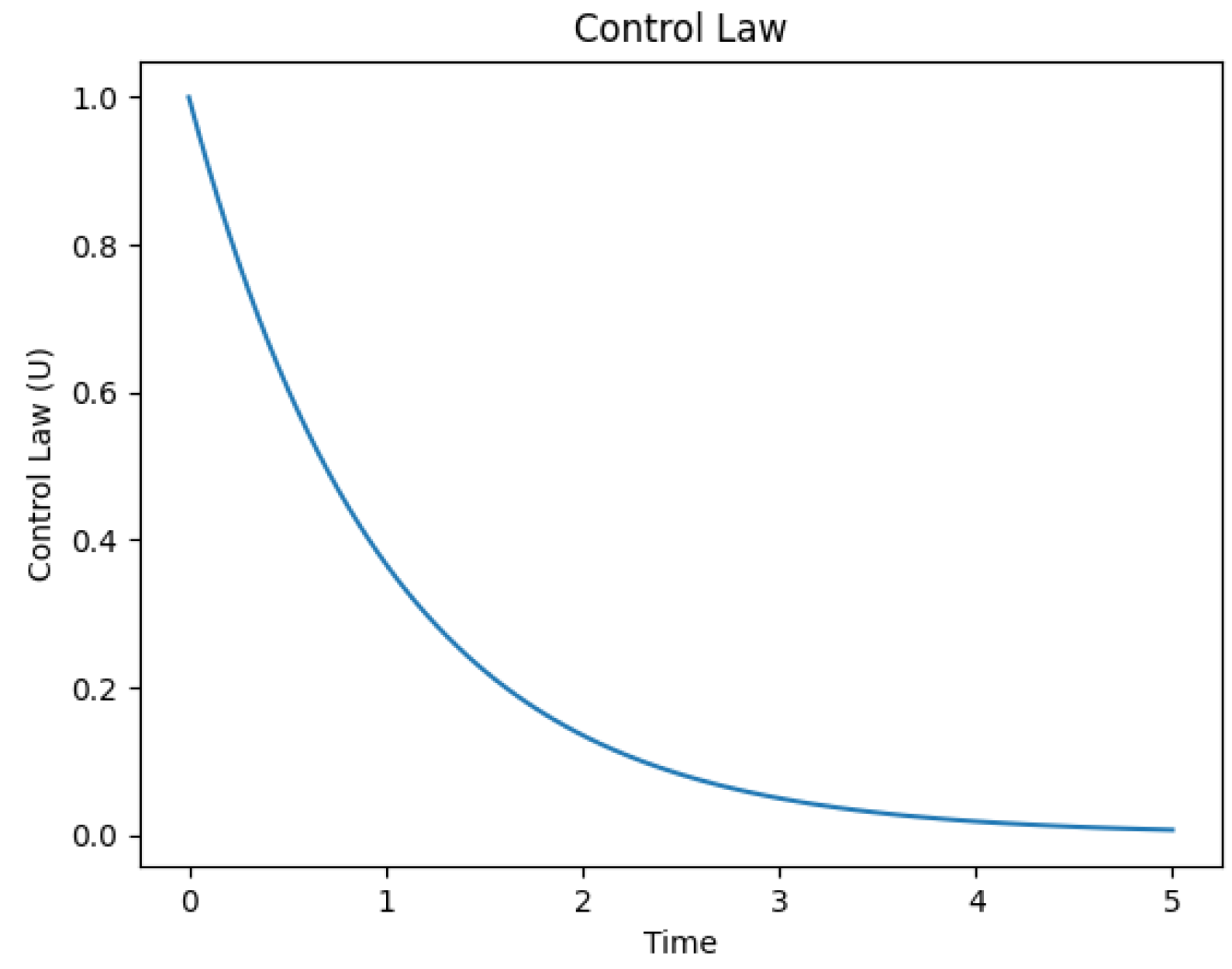
At the same time, in order to make the trajectory of the error system reach the sliding mode surface, another arrival control law is added as follows:

$$\begin{array}{c}\hfill u_{ac}\left(t\right)=-\gamma sgn{\left(S\left(t\right)\right)}^{2\xi -1},\end{array}$$

(15)

where $\gamma >0$ represents the switching gain. Therefore, in this paper, the control law combining (14) and (15) is designed as follows (Figure 2):

$$\begin{array}{cc}\hfill U\left(t\right)=& u_{eq}\left(t\right)+u_{ac}\left(t\right)\hfill \\ \hfill =& -(KP+\overline{\Omega }+Q-\Omega )e\left(t\right)-\alpha (\overline{\Omega }-\Omega )\overline{L}(t-\beta )+\alpha \overline{R}\overline{F}\left(\overline{L}(t-\beta )\right)\hfill \\ \hfill & -RF\left(\alpha \overline{L}(t-\beta )\right)-\Xi sign\left(e\left(t\right)\right)-\gamma sgn{\left(S\left(t\right)\right)}^{2\xi -1}\hfill \end{array}$$

(16)

After the design of sliding mode control law, it is necessary to discuss the reachability of the sliding mode surface.

3.5. Reachability Analysis in Finite Time

Theorem 1. 

Suppose there is a sliding mode surface described by formula (9), and then the error system (7) can reach the sliding mode surface $S\left(t\right)=0$ in a finite time T under the sliding mode control law (16), whose calculation formula is

$$\begin{array}{c}\hfill T={\left(V_1^{\frac{\overline{\omega }(\mu +1)-1}{\mu }-\xi }\left(0\right)\frac{\eta \mu \Gamma (1+\overline{\omega })\Gamma \left(\frac{(1-\xi )\mu }{\mu +1}\right)}{2\gamma (1+\mu )\Gamma (\overline{\omega }+\frac{(1-\xi )\mu }{\mu +1})}\right)}^{\frac{1}{\overline{\omega }}},\end{array}$$

where $0<\underline{\omega }\le \omega \left(t\right)\le \overline{\omega }<1$, $\eta =\frac{\Gamma (1-\overline{\omega })}{\Gamma (1-\underline{\omega })}$, $\xi =\frac{\mu (\sigma -1)-1}{\mu (1+\mu +\sigma )}$, $\sigma =2\tau +1$, $\mu =2\varsigma -1$, $\tau ,\varsigma \in {\mathbb{N}}_{+}$, $0<\frac{1+\xi \mu }{1+\mu }<\overline{\omega }$, $V_1\left(0\right)=\frac{1}{2}{\displaystyle \sum _{i=1}^{nN}}|s_i\left(0\right){|}^2$.

Proof. 

Consider the following Lyapunov candidate function:

$$V_1\left(t\right)=\frac{1}{2}\sum _{i=1}^{nN}{\left|s_i\left(t\right)\right|}^2=\frac{1}{2}{S}^T\left(t\right)S\left(t\right).$$

(17)

According to Lemma 1, the VOFD of Lyapunov candidate function (17) along sliding mode surface (10) satisfies

$$J^{\omega \left(t\right)}{V}_1\left(t\right)\le S^T\left(t\right)J^{\omega \left(t\right)}S\left(t\right).$$

(18)

Substituting (11) into (18), one has

$$\begin{array}{c}{J}^{\omega \left(t\right)}{V}_1\left(t\right)\le S^T\left(t\right)((KP+\overline{\Omega }+Q-\Omega )e\left(t\right)+U\left(t\right)+\alpha (\overline{\Omega }-\Omega )\overline{L}(t-\beta )\hfill \\ -\overline{R}\left[\alpha \overline{F}\left(\overline{L}(t-\beta )\right)\right]+RF\left(\alpha \overline{L}(t-\beta )\right)+\Xi sign\left(e\left(t\right)\right)).\hfill \end{array}$$

(19)

Next, substituting (16) into (19), it is easy to obtain

$$\begin{array}{cc}\hfill J^{\omega \left(t\right)}{V}_1\left(t\right)\le & -\gamma S^T\left(t\right)sgn{\left(S\left(t\right)\right)}^{2\xi -1}=-\gamma \sum _{i=1}^{nN}{\left|s_i\left(t\right)\right|}^{2\xi }=-\gamma \sum _{i=1}^{nN}{\left[{\left|s_i\left(t\right)\right|}^2\right]}^{\xi },\hfill \end{array}$$

(20)

where $\gamma >0$ is the switching gain. Using Lemma 2, formula (20) can be transformed into

$$J^{\omega \left(t\right)}{V}_1\left(t\right)\le -\gamma {\left[\sum _{i=1}^{nN}{\left|s_i\left(t\right)\right|}^2\right]}^{\xi }=-2\gamma V_1^{\xi }\left(t\right).$$

(21)

Then, one can obtain it from formula (21) and Lemma 3 that

$$\underset{t\to T}{lim}∥s_i\left(t\right)∥=0,s_i\left(t\right)=0,t\ge T,$$

(22)

where

$$T={\left(V_1^{\frac{\overline{\omega }(\mu +1)-1}{\mu }-\xi }\left(0\right)\frac{\eta \mu \Gamma (1+\overline{\omega })\Gamma \left(\frac{(1-\xi )\mu }{\mu +1}\right)}{2\gamma (1+\mu )\Gamma (\overline{\omega }+\frac{(1-\xi )\mu }{\mu +1})}\right)}^{\frac{1}{\overline{\omega }}}.$$

Based on Lyapunov stability theory, from formula (22), it can be seen that the error system (7) can be driven to the sliding mode surface in a limited time T and will remain on the sliding mode surface $S\left(t\right)=0$ in the subsequent time. □

Remark 4. 

The SMC control strategy is also used in [22] for finite time reachability analysis, but the finite time range is given by inequality $T_f^{*}\le V_1^{1/2}\left(0\right)/\left(\rho \sqrt{2/{\lambda }_{max}{\left(LB\right)}^{-1}}\right)$, and the specific expression is given by Theorem 1. For detailed explanation, see Example 1.

After the error system (9) reaches the sliding mode surface in a finite time, the control law $u_{ac}\left(t\right)=-\gamma sgn{\left(S\left(t\right)\right)}^{2\xi -1}=0$, and then the total control law $u_{eq}\left(t\right)+u_{ac}\left(t\right)$ can be written as

$$\begin{array}{cc}\hfill U\left(t\right)=& -(KP+\overline{\Omega }+Q-\Omega )e\left(t\right)-\alpha (\overline{\Omega }-\Omega )\overline{L}(t-\beta )+\alpha \overline{R}\overline{F}\left(\overline{L}(t-\beta )\right)\hfill \\ \hfill & -RF\left(\alpha \overline{L}(t-\beta )\right)-\Xi sign\left(e\left(t\right)\right).\hfill \end{array}$$

(23)

Now, it is time to discuss the evolution of this synchronization error system after reaching the sliding surface.

3.6. Synchronization Analysis

Substituting the control law (23) into the error system (9), one obtains

$$\begin{array}{cc}\hfill J^{\omega \left(t\right)}e\left(t\right)=& -\Omega e\left(t\right)+RF\left(e\left(t\right)\right)-(KP+\overline{\Omega }+Q-\Omega )e\left(t\right)-\alpha (\overline{\Omega }-\Omega )\overline{L}(t-\beta )\hfill \\ \hfill & +\alpha \overline{R}\overline{F}\left(\overline{L}(t-\beta )\right)-RF\left(\alpha \overline{L}(t-\beta )\right)-\Xi sign\left(e\left(t\right)\right)+\alpha (\overline{\Omega }-\Omega )\times \hfill \\ \hfill & \overline{L}(t-\beta )-\overline{R}\left[\alpha \overline{F}\left(\overline{L}(t-\beta )\right)\right]+RF\left(\alpha \overline{L}(t-\beta )\right)\hfill \\ \hfill =& -(KP+\overline{\Omega }+Q)e\left(t\right)+RF\left(e\left(t\right)\right)-\Xi sign\left(e\left(t\right)\right),\hfill \end{array}$$

(24)

It is not difficult to know that $e^{*}=0$ is an equilibrium point of system (24), and then comes the asymptotic stability of this system.

Theorem 2. 

If there are two constants $\epsilon >0$ and $\delta >0$, a gain matrix $K\in {\mathbb{R}}^{nN\times M}$, two diagonal matrices $Q=diag{\left(q_i\right)}_{nN}$, and $\Xi =diag{\left({\theta }_i\right)}_{nN}$ can satisfy formula (25), then the response system (2) and the driving system (4) can achieve asymptotically hybrid projection lag synchronization:

$$\epsilon R{R}^T+\frac{{\lambda }^2+\delta \epsilon }{\epsilon }{I}_{nN}-(KP+P^T{K}^T+\overline{\Omega }+{\overline{\Omega }}^T+Q+Q^T+\frac{1}{\delta }\Xi {\Xi }^T)<0,$$

(25)

where $\lambda =\underset{i=1,...,n}{max}\left\{{\lambda }_i\right\}$, P is the output transient matrix, $\Omega =\left(I_N\otimes A\right)-(CD\otimes G),\overline{\Omega }=\left(I_N\otimes \overline{A}\right)-(\overline{C}\overline{D}\otimes \overline{G}),R=\left(I_N\otimes B\right)$ and $\overline{R}=\left(I_N\otimes \overline{B}\right).$

Proof. 

Considering the following Lyapunov candidate function:

$$V_2\left(t\right)=\frac{1}{2}{e}^T\left(t\right)e\left(t\right),$$

(26)

According to Lemma 1, the VOFD inequality of Lyapunov candidate function (26) along error system (24) is obtained

$$\begin{array}{cc}\hfill J^{\omega \left(t\right)}{V}_2\left(t\right)& \le e^T\left(t\right)J^{\omega \left(t\right)}e\left(t\right)\hfill \\ \hfill & =-e^T\left(t\right)(KP+\overline{\Omega }+Q)e\left(t\right)+e^T\left(t\right)RF\left(e\left(t\right)\right)-e^T\left(t\right)\Xi sign\left(e\left(t\right)\right),\hfill \end{array}$$

(27)

Then, for the second term of formula (27), using Lemma 4, there is a constant $\epsilon >0$ such that

$$e^T\left(t\right)RF\left(e\left(t\right)\right)\le \frac{\epsilon }{2}{e}^T\left(t\right)R{R}^{T}e\left(t\right)+\frac{1}{2\epsilon }{\left[F\left(e\left(t\right)\right)\right]}^T\left[F\left(e\left(t\right)\right)\right],$$

(28)

Combining with Assumption 1, formula (28) can be transformed into

$$e^T\left(t\right)RF\left(e\left(t\right)\right)\le e^T\left(t\right)\left[\frac{\epsilon }{2}R{R}^T+\frac{{\lambda }^2}{2\epsilon }{I}_{nN}\right]e\left(t\right).$$

(29)

Similarly, for the third term of formula (27), using Lemma 4, there is a constant $\delta >0$ such that

$$-e^T\left(t\right)\Xi sign\left(e\left(t\right)\right)\le e^T\left(t\right)\left(\frac{\delta }{2}{I}_{nN}+\frac{1}{2\delta }\Xi {\Xi }^T\right)e\left(t\right).$$

(30)

Substituting (29) and (30) into (27), one can obtain

$$\begin{array}{c}\hfill J^{\omega \left(t\right)}{V}_2\left(t\right)\le -e^T\left(t\right)(KP+\overline{\Omega }+Q-\frac{\epsilon }{2}R{R}^T-\frac{{\lambda }^2+\delta \epsilon }{2\epsilon }{I}_{nN}+\frac{1}{2\delta }\Xi {\Xi }^T)e\left(t\right),\end{array}$$

(31)

Denote $\Phi =KP+P^T{K}^T+\overline{\Omega }+{\overline{\Omega }}^T+Q+Q^T+\frac{1}{\delta }\Xi {\Xi }^T-\epsilon R{R}^T-\frac{{\lambda }^2+\delta \epsilon }{\epsilon }{I}_{nN}$, and ${\varphi }_{min}$ is the minimum eigenvalue of symmetric matrix $\Phi$, and then (31) can be written as

$$J^{\omega \left(t\right)}{V}_2\left(t\right)\le -{\varphi }_{min}{V}_2\left(t\right),$$

(32)

According to Lemma 5, from (32), one can obtain

$$J^{\overline{\omega }}{V}_2\left(t\right)\le -\frac{{\varphi }_{min}}{\eta }{V}_2\left(t\right),$$

(33)

where $\eta =\frac{\Gamma (1-\overline{\omega })}{\Gamma (1-\underline{\omega })}.$

From Lemma 6, it can be derived combining with (33) that

$$V_2\left(t\right)\le V_2\left(0\right)E_{\overline{\omega }}(-\frac{{\varphi }_{min}}{\eta }{t}^{\overline{\omega }}),$$

(34)

where $V_2\left(0\right)=\frac{1}{2}{e}^T\left(0\right)e\left(0\right)$.

Considering the definition of Lyapunov candidate function (26), it can be obtained from (34) that

$$\left|\right|e\left(t\right)\left|\right|\le {\left[2V_2\left(0\right)E_{\overline{\omega }}(-\frac{{\varphi }_{min}}{\eta }{t}^{\overline{\omega }})\right]}^{1/2}.$$

(35)

Take the limit on both sides of formula (35); from the pinch theorem, one can obtain that ${lim}_{t\to +\infty }\parallel e\left(t\right)\parallel =0$.

All in all, the error system will achieve global asymptotic stability, which means that the response system (2) and the driving system (4) can achieve asymptotic hybrid projection lag synchronization. □

Corollary 1. 

Let ω be a constant; if $\omega \left(t\right)\equiv \omega$, and $\overline{c}=0$, the models considered in this paper degenerate into the model with constant-order fractional derivative and decoupled driving system network in [13]. If $\alpha =I_{nN}$ and $\beta =0$, the asymptotical hybrid projection lag synchronization degenerates to the ordinary asymptotical synchronization in the previous reference.

4. Illustrative Examples

The methods of numerical simulation used in this section can be found in Refs. [23,34,35]. In this section, two simulation examples based on Matlab are presented. The parameters of these two simulation examples are derived from Refs. [8,13], respectively.

Example 1. 

For the convenience of simulation experiments, a class of $N=3$ and $n=2$ variable-order fractional driving and response system described by (2) and (4) are considered, and the related parameters are assigned as follows:

$$\begin{array}{c}\hfill \overline{A}=\left[\begin{array}{cc}0.7& 0\\ 0& 0.8\end{array}\right],\overline{B}=\left[\begin{array}{cc}-0.1& 0.3\\ 0.3& -0.2\end{array}\right],A=\left[\begin{array}{cc}\hfill 0.6& 0\\ \hfill 0& 0.7\end{array}\right],B=\left[\begin{array}{cc}\hfill -0.2& 0.4\\ \hfill 0.4& -0.1\end{array}\right],\\ \overline{C}=\left[\begin{array}{ccc}0.31& 0& 0\\ 0& 0.32& 0\\ 0& 0& 0.33\end{array}\right],C=\left[\begin{array}{ccc}\hfill 0.21& 0& 0\\ \hfill 0& 0.22& 0\\ \hfill 0& 0& 0.23\end{array}\right],D=\left[\begin{array}{ccc}\hfill 0.47& 0.90& 0.42\\ \hfill 0.90& -0.35& -0.30\\ \hfill 0.42& -0.30& 0.35\end{array}\right],\hfill \\ \overline{D}=\left[\begin{array}{ccc}\hfill 0.047& 0.090& 0.042\\ \hfill 0.090& -0.035& -0.030\\ \hfill 0.042& -0.030& 0.035\end{array}\right],\overline{G}=\left[\begin{array}{cc}\hfill 2& 0\\ \hfill 0& 2\end{array}\right],G=\left[\begin{array}{cc}1& 0\\ 0& 3\end{array}\right],\alpha =2I_6,\hfill \end{array}$$

$\beta =1$, $\omega \left(t\right)=-0.5+\frac{1.4}{1+e^{-t}}$, $f_i={\overline{f}}_i=tanh\left(x\right),i=1,2,...,n.$ It is easy to know that $\underline{\omega }=0.2$, $\overline{\omega }=0.9$, and ${\lambda }_i={\overline{\lambda }}_i=1$.

The initial values of the driving system and the response system are generated randomly. The phase diagram and synchronization error evolution diagram of the driving and response system without control protocol are shown in Figure 3 and Figure 4, respectively.

It can be seen from Figure 3 and Figure 4 that the response system has great freedom when it does not receive the control protocol and will not actively synchronize with the driving system. Then, in order to enable the response system to achieve the goal of asymptotic hybrid projection lag synchronization, the design of a control protocol is necessary. The following is the selection of parameters: $\epsilon =1$, $\delta =0.3$, $\gamma =5$, $\Xi =diag{\left({\theta }_i\right)}_6$, where the value of ${\theta }_i$ is 0.153, 0.159, 0.037, 0.098, 0.089, and 0.129 in the order of increasing i, and $P=\left(\begin{array}{cc}{P}_1& P_2\end{array}\right)$, $K=\left(\begin{array}{c}{K}_1\\ K_2\end{array}\right)$, $Q=\left(\begin{array}{cc}{Q}_{11}& Q_{12}\\ Q_{21}& Q_{22}\end{array}\right)$, where

$P_1=\left[\begin{array}{ccc}\hfill 0.3575& -0.2155& 0.4121\\ \hfill 0.5155& 0.3110& -0.9363\\ \hfill 0.4863& -0.6576& -0.4462\end{array}\right]$, $P_2=\left[\begin{array}{ccc}\hfill -0.9077& 0.3897& -0.9311\\ \hfill -0.8057& -0.3658& -0.1225\\ \hfill 0.6469& 0.9004& -0.2369\end{array}\right]$,

$K_1=\left[\begin{array}{ccc}\hfill 0.1912& 0.7573& 0.6576\\ \hfill -0.2661& 0.3609& -0.7330\\ \hfill 0.5322& -0.9400& -0.5188\end{array}\right]$, $K_2=\left[\begin{array}{ccc}\hfill -0.6490& -0.4372& 0.4708\\ \hfill 0.3579& -0.3399& 0.7693\\ \hfill -0.9581& 0.0462& -0.1160\end{array}\right]$,

$Q_{11}=\left[\begin{array}{ccc}\hfill 0.7418& 0.2518& 0.7353\\ \hfill 0.2518& 0.8687& 0.0932\\ \hfill 0.7353& 0.0932& 0.1893\end{array}\right]$, $Q_{12}=\left[\begin{array}{ccc}\hfill 0.2934& -0.3581& 0.4008\\ \hfill 0.4148& 0.7922& -0.3371\\ \hfill 0.0647& -0.1033& 0.3219\end{array}\right]$,

$Q_{21}=\left[\begin{array}{ccc}\hfill 0.2934& 0.4148& 0.0647\\ \hfill -0.3581& 0.7922& -0.1033\\ \hfill 0.4008& -0.3371& 0.3219\end{array}\right]$, $Q_{22}=\left[\begin{array}{ccc}\hfill 0.2742& -0.3888& -0.6519\\ \hfill -0.3888& 0.5638& 0.4842\\ \hfill -0.6519& 0.4842& 0.6064\end{array}\right]$.

Use the LMI toolbox of MATLAB to solve and verify that the above parameters are feasible solutions. After the control protocol is applied to the response system, according to the finite time calculation formula provided in Theorem 1, the time to reach the sliding mode surface is $T=3.4403$, and the evolution of the synchronization error system is shown in Figure 5.

It can be seen from Figure 5 that the response system can reach the sliding mode surface in a finite time under the action of the control protocol and realize hybrid projection lag synchronization with the driving system along the sliding mode surface.

Remark 5. 

Theorem 2 in Ref. [8] provides a sufficient condition for asymptotic synchronization of driving and response systems, in which there are two inequality constraints, while the sufficient conditions provided in this paper are freer.

Remark 6. 

The finite time using the traditional SMC method provided in Ref. [22] is in the form of inequality. In terms of Example 1, the calculated range is $T_f^{*}\le 7.7997$. Obviously, this estimation is too conservative and $T=3.4403$ is more accurate.

Example 2. 

In order to further illustrate that the model considered is more general, a class of $N=3$ and $n=2$ variable-order fractional driving and response system described by (2) and (4) is considered, and the related parameters are assigned as follows: $A=\overline{A}=C=G=I_3$, $\overline{C}=\overline{D}=\overline{G}=O_3$, $\alpha =I_9$, $\beta =0$, $B=\overline{B}=\left[\begin{array}{ccc}\hfill 2.0& -1.2& 0\\ \hfill 1.8& 1.71& 1.15\\ \hfill -4.75& 0& 1.1\end{array}\right]$, $D=\left[\begin{array}{ccc}\hfill -1& 0& 0\\ \hfill 1& -2& 0\\ \hfill 0& 1& -1\end{array}\right]$, $\omega \left(t\right)\equiv 0.98$,$f_i={\overline{f}}_i=tanh\left(x\right)$, $i=1,2,...,n$, $\epsilon =1$, $\gamma =7$, $\Xi =diag{\left({\theta }_i\right)}_9$, where the value of ${\theta }_i$ is 0.0098, 0.0044, 0.0011, 0.0026, 0.0041, 0.0059, 0.0026, 0.0060, and 0.0071 in the order of increasing i, and $P,K,Q$ are $9\times 9$ matrices shown in

Table 1. Solution of corresponding LMI in Example 2.

Matrix	Solution
P	$\left[\begin{array}{ccccccccc}\hfill -0.0196& 0.0890& -0.0517& -0.0294& 0.0094& -0.0838& 0.0635& 0.0100& -0.0548\\ \hfill -0.0848& -0.0018& -0.0192& 0.0642& -0.0407& 0.0859& 0.0590& 0.0245& -0.0659\\ \hfill -0.0520& -0.0021& -0.0807& -0.0969& 0.0489& 0.0551& 0.0289& 0.0174& -0.0545\\ \hfill -0.0753& -0.0325& -0.0736& -0.0914& -0.0622& -0.0026& -0.0243& -0.0585& -0.0129\\ \hfill -0.0632& 0.0800& 0.0884& -0.0662& 0.0374& -0.0128& 0.0623& -0.0398& -0.0378\\ \hfill -0.0520& -0.0262& 0.0912& 0.0298& -0.0633& -0.0106& 0.0066& -0.0058& 0.0847\\ \hfill -0.0165& -0.0778& 0.0150& 0.0463& -0.0263& -0.0387& -0.0299& -0.0539& -0.0140\\ \hfill -0.0901& 0.0561& -0.0880& 0.0295& 0.0251& 0.0017& 0.0878& 0.0689& -0.0630\\ \hfill 0.0805& -0.0221& -0.0530& -0.0098& 0.0560& 0.0022& 0.0752& -0.0610& 0.0810\end{array}\right]$
K	$\left[\begin{array}{ccccccccc}\hfill 145.80& 79.088& 77.079& -79.828& -71.839& 15.825& -12.468& -173.34& 14.939\\ \hfill -126.43& -40.416& -222.50& 118.24& 89.133& -124.37& -130.70& 127.27& -1.154\\ \hfill 58.055& 30.486& 77.272& -80.637& 13.788& 64.511& 29.600& -93.234& -25.238\\ \hfill -119.53& -18.121& -156.38& 38.889& 38.380& -82.348& 10.079& 131.66& 13.574\\ \hfill -172.27& -121.96& -46.489& 3.167& 85.636& -79.835& 38.143& 168.52& 14.598\\ \hfill -98.915& 51.332& -48.070& 39.508& 30.623& -57.136& -77.755& 7.144& 14.930\\ \hfill 194.74& 109.81& 162.78& -108.03& -56.043& 125.62& 41.48& -145.89& 49.456\\ \hfill 128.85& 10.430& 175.28& -122.77& -107.76& 127.32& -3.601& -80.865& -52.952\\ \hfill -117.69& -82.994& -91.145& 68.060& 20.011& 18.733& -68.183& 119.56& 36.519\end{array}\right]$
Q	$\left[\begin{array}{ccccccccc}\hfill 0.0082& -0.0168& 0.0084& -0.0133& -0.0164& -0.0044& 0.0196& 0.0144& -0.0123\\ \hfill -0.0168& 0.0150& -0.0126& 0.0184& 0.0156& 0.0102& -0.0267& -0.0230& 0.0153\\ \hfill 0.0084& -0.0126& 0.0034& -0.0087& -0.0080& -0.0039& 0.0124& 0.0102& -0.0075\\ \hfill -0.0133& 0.0184& -0.0087& 0.0072& 0.0137& 0.0057& -0.0186& -0.0161& 0.0103\\ \hfill -0.0164& 0.0156& -0.0080& 0.0137& 0.0098& 0.0041& -0.0200& -0.0144& 0.0116\\ \hfill -0.0044& 0.0102& -0.0039& 0.0057& 0.0041& 0.0029& -0.0083& -0.0081& 0.0045\\ \hfill 0.0196& -0.0267& 0.0124& -0.0186& -0.0200& -0.0083& 0.0144& 0.0216& -0.0156\\ \hfill 0.0144& -0.0230& 0.0102& -0.0161& -0.0144& -0.0081& 0.0216& 0.0109& -0.0112\\ \hfill -0.0123& 0.0153& -0.0075& 0.0103& 0.0116& 0.0045& -0.0156& -0.0112& 0.0060\end{array}\right]$

.

In this study, the synchronization approach was tested by randomly generating initial values for both the driving and response systems. The results of the control protocol were then analyzed using phase diagrams for the first node of the driving and response chaotic systems (Figure 6), as well as a chaotic synchronization error evolution diagram (Figure 7).

Firstly, the phase diagram of a chaotic system displays specific characteristics of the chaotic signal, such as frequency and amplitude. Therefore, Figure 6 shows that the output of the first node of the driver as well as the chaotic system where the control is implemented converge to the expected output value, indicating the effectiveness of the control protocol in Theorem 2.

Secondly, Figure 7 demonstrates the efficiency and stability of the control protocol in Theorem 2 by evaluating its effectiveness through the synchronization error between the two chaotic system nodes at each time step. The synchronization error gradually decreases over time and eventually tends to zero, indicating that the driver system and response system achieve asymptotic synchronization under the conditions of Theorem 2. This result is promising as it demonstrates the efficacy of the proposed variable-order fractional integral sliding mode surface approach in achieving synchronization in nonidentical VOFD complex networks.

Therefore, phase diagrams and chaotic synchronization error evolution diagrams are useful tools for analyzing control protocol results. These tools can be used to guide control protocol optimization and improve the control efficiency and stability of the chaotic system. It should be noted that, due to the highly complex and uncertain behavior of chaotic systems, several factors need to be carefully considered when designing control protocols. Additionally, to further validate the effectiveness of the proposed approach, more extensive experiments and numerical simulations are required for complex networks.

It should be noted that the use of phase diagrams and chaotic synchronization error evolution diagrams is a common practice in studies involving synchronization analysis. These visual representations provide a clear and intuitive way to understand the dynamics of the systems under investigation.

Remark 7. 

The sufficient conditions for the asymptotic synchronization of the driving and response system are provided in the literature [13]. The system parameters of Example 2 are from this literature. It is well illustrated that the model considered in this paper is more general.

5. Conclusions

This paper presents a novel technique for achieving synchronization in nonidentical variable-order fractional differential (VOFD) complex networks. Specifically, the proposed approach uses a variable-order fractional integral sliding mode surface to enable the driving and response systems to reach asymptotic hybrid projection lag synchronization. By leveraging the power of mathematical concepts such as fractional calculus inequality and comparison theorem, this study establishes the sufficient conditions for asymptotic hybrid projection lag synchronization of the VOFD complex networks.

The use of fractional calculus is especially relevant when analyzing systems that involve fractional derivatives or integrals and can provide a more precise understanding of the dynamics of such systems. By applying these mathematical tools, the authors were able to derive conditions that ensure the stability and convergence of the synchronization process in the VOFD complex networks.

The results of this study complement and build upon previous findings in the field of VOFD complex networks synchronization. The proposed method extends these results to special cases, such as lag synchronization and anti-synchronization of COFD complex networks, as well as the projection synchronization of the same variable-order fractional networks. This demonstrates the versatility and efficacy of the proposed synchronization approach.

The potential applications of this research are many-fold, including areas such as microbial metabolic regulation. The authors suggest that future work should focus on investigating the synchronization of nonidentical VOFD complex dynamic networks in a more general order and exploring their use in achieving finite time or fixed time synchronization.

The simple design advantage of sliding mode control is worthy of note, but it is crucial to acknowledge the potential disadvantage of the chattering phenomenon in the controller’s control input. This phenomenon, which can result in high-frequency oscillations in the control signal, may be undesirable in some practical applications. To address this issue, we have explored various methods for reducing or eliminating chattering, such as using a differentiable sign function or introducing a switching function with hysteresis.

Overall, this paper offers valuable insights into the synchronization of complex systems involving variable-order fractional derivatives or integrals. The proposed method is expected to have broad applicability in various real-world scenarios, and the future research directions suggested by the authors are promising. As such, this study makes an important contribution to the field of complex network synchronization and serves as a basis for further studies in this area.