On Incidence-Dependent Management Strategies against an SEIRS Epidemic: Extinction of the Epidemic Using Allee Effect

Abstract

We developed a mathematical model to study the effects of non-pharmaceutical interventions (NPIs) on the dynamics of an epidemic. The level of intervention was assessed as a fraction of the population being isolated and depended on the level of incidence of the epidemic in the population. We performed a mathematical analysis of the model and showed that, depending on the choice of the prevalence-dependent isolation function, it is possible to create new endemic equilibria and to change the stability of the disease-free equilibrium for which the epidemic vanishes. The model was then applied to the case of the COVID-19 pandemic. Several NPI management strategies were considered. In the case of an NPI intensity increasing with the level of infection, it is possible to avoid the initial epidemic peak of great amplitude that would have occurred without intervention and to stabilize the epidemic at a chosen and sufficiently low endemic level. In the case of an NPI intensity decreasing with the level of infection, the epidemic can be driven to extinction by generating an “Allee” effect: when the incidence is below a given level, the epidemic goes extinct whereas, above it, the epidemic will still be able take hold at a lower endemic level. Simulations illustrate that appropriate NPIs could make the COVID-19 vanish relatively fast. We show that, in the context of the COVID-19 pandemic, most countries have not chosen to use the most efficient strategies.

1. Introduction

We present here a theoretical approach aiming at evaluating the effects of some non-pharmaceutical interventions (NPIs) such as lockdown, social distancing or teleworking in order to limit the number of cases. We discuss their ability to fulfill some requirements such as keeping the number of cases at a level low enough to be managed by hospitals or maintaining a lockdown at a level low enough to avoid consequences that are too damaging to the economy. We are also looking for NPI measures in order to bring about the eradication of the epidemic. In SIRS and SEIRS classical epidemic models, there exist a disease-free equilibrium (DFE) and a single endemic equilibrium (EE) that can be positive depending on the values of the parameters. A basic reproduction number of the epidemic ${\mathcal{R}}_0$ is defined and represents the number of people infected by a single infectious person during their illness. According to the value of this parameter, there are two cases: either ${\mathcal{R}}_0$ is smaller than 1 and the epidemic goes extinct, i.e., the DFE is globally stable while the EE does not exist, or the epidemic takes hold, i.e., ${\mathcal{R}}_0$ is greater than 1, the DFE is unstable and the EE is globally stable.

The aim of this work was to propose NPI protection measures depending on the number of infected people to control and eradicate an epidemic. Therefore, a proportion of protected people is defined by function $v\left(I\right)$. Such infected-dependent protection measures significantly allow for modifying the global phase portrait by creating several endemic equilibria depending on the particular choice of the function $v\left(I\right)$. We particularly considered choices of the protection function that allow for bringing about the extinction of the epidemic. In particular, we focused on a class of protection functions that generate an “Allee” effect. The Allee effect is well known in population dynamics and ecology [1]. A commonly accepted definition of the Allee effect is a positive density dependence of the growth rate per capita. More precisely, the demographic Allee effect is the positive relationship between the overall individual fitness and population density. The weak Allee effect keeps the population growth rate quite low but positive at a low density whereas the strong Allee effect induces a negative growth rate below a certain threshold [2,3]. It can generally be observed and has high significance at a low population level, and it is often used to explain tipping points, as a low or negative growth rate may result in the extinction of endangered species. The Allee effect aims at taking into account the difficulties in mating or the absence of cooperative behavior (defense, feeding) between individuals at a low density causing the eradication of the species: panda populations hardly grow, partly because of a very low birthrate; fish stocks may be unable to recover from overfishing. In order to grow, the initial population must be at a sufficiently high density above this threshold. In the case of a harvested population, a high price of the resource due in particular to its scarcity can also induce an Allee effect [4].

Equivalently, such an effect could happen in an epidemiology context, when the number of infected people is too small to start a wave of infection. While an Allee effect is generally not desirable in ecology, creating the conditions of such an effect would be a great asset in order to mitigate an epidemic. A judicious choice of functions $v\left(I\right)$ allows for generating two endemic equilibria, one at a low level, denoted EE1, and the other at a higher endemic level, denoted EE2. By analogy, the case where EE1 is unstable while EE2 is stable corresponds to an “Allee” effect. According to the basins of attraction of equilibria, we can create a situation where any initial condition chosen below the level of infection of EE1 can lead to the eradication of the epidemic whereas, for any initial condition above, the epidemic settles and stabilizes in the long term at the level of EE2. In this work, we focused on a class of functions $v\left(I\right)$ allowing us to generate such an Allee effect as well as any other class of functions allowing us to cause the extinction of the epidemic.

The article is made up of seven sections. After an introductory part, Section 2 presents a general SEIRS epidemic model with infected-dependent control and a mathematical analysis of the epidemic model, such as the existence of endemic equilibria and stability properties. In Section 3, we discuss the application of the model to the SARS-CoV-2 epidemic. In Section 4, we compare several infection-dependent NPI strategies. Among these, we present a constant level strategy, a strategy used to avoid a large-scale epidemic peak and to stabilize the epidemic at an endemic level low enough to avoid congestion in hospitals and strategies that allow for generating an Allee effect that permits the provoking of the extinction of the epidemic below some endemic threshold. Section 5 is devoted to identifying which strategies have been used against COVID-19. Section 6 presents a discussion of the results with a comparison of the different strategies showing the advantages, limitations and costs of each one. We conclude in Section 7.

2. An SEIRS Model with NPI Depending on the Number of Infected People

In the following model, the population is distributed among four compartments that are almost equivalent to those of a classical SEIRS model: a compartment S with susceptible individuals, a compartment E with exposed individuals, a compartment I with both asymptomatic (infectious without symptoms onset) and pre-symptomatic (infectious before symptoms onset or test) individuals and a compartment R, which contains individuals that have been removed from the infection dynamics, i.e., asymptomatic individuals after recovery, and symptomatic individuals who are assumed to be quarantined as soon as they get aware of their condition (symptoms onset or positive test). We assumed a constant total population $N=S+E+I+R$ since the time scale of the epidemic is small compared to the one of population growth.

We considered an epidemic focus, such as a country where the epidemic has just started. It is normally necessary to take into account the urban mobility of individuals in the dynamics of the epidemic. We cite the work [5], in which aged structured individuals are supposed to move between their place of residence, workplaces, universities, schools, public places, shopping centers and more places [6,7]. In a previous model [8], we also took into account the daily movements of people between their home and the various places where they are required to move and where they are more or less protected from contact with infectious persons as well as lockdown and protection by masks following the work by [9].

We assumed that individuals can switch between a normal state and a state in which they are removed from the dynamics because of NPI, such as isolation, lockdown or social distancing. Thus, NPIs result in a proportion v of the population being in a state of isolation. For example, an NPI that imposes two days of teleworking per labor week (five days) would result in a proportion $v=40\%$ of isolated people working from home every day. However, people may be in a different state every day. In the following sections, v will refer to a more general definition of NPI intensity that will not only apply to lockdown or teleworking but also to social distancing or mask wearing by assuming that any measure is equivalent to a percentage of time spent in isolation. It should be noticed that measures such as lockdown, stay-at-home or curfew apply to the whole population independent of their infection status.

Infected individuals follow the natural process of the disease corresponding to a classical SEIRS model, i.e., exposed individuals can become infected after an incubation time $\frac{1}{k}$. Infected individuals are removed after an average time $\frac{1}{\alpha }$, either because they recovered or because they have been tested or are symptomatic and thus quarantined. They lose their immunity after a time $\frac{1}{\gamma }$. The number of newly infected individuals per unit of time for the population in a classical SEIRS model is given by the expression $\beta \frac{SI}{N}$, where $\beta$ is the transmission rate of the disease for one infectious individual in a population with only susceptible individuals. Since the same NPI rules apply to susceptible and asymptomatic/presymptomatic individuals, only a proportion $1-v$ of both S and I is involved in the disease transmission. Thus, this expression must be replaced by $\beta \frac{(1-v)S(1-v)I}{N}$. A detailed justification of this formula is presented in Appendix B. Figure 1 illustrates the reduction in the number of infections: without NPI, four infections occur. With NPI, a proportion $v=0.5$ of the population is isolated (shaded area) and cannot be infected or infect others. Compared to the case without NPI, infections can only occur between two persons outside of the shaded area; thus, the ones with a red cross cannot occur any more. The number of infections is reduced to ${(1-v)}^2=0.25$ of the original infections.

The modified SEIRS model reads

$$\left\{\begin{array}{ccc}\hfill \frac{dS}{dt}& =& -\beta {(1-v)}^2\frac{SI}{N}+\gamma R,\hfill \\ \hfill \frac{dE}{dt}& =& \beta {(1-v)}^2\frac{SI}{N}-kE,\hfill \\ \hfill \frac{dI}{dt}& =& kE-\alpha I,\hfill \\ \hfill \frac{dR}{dt}& =& \alpha I-\gamma R.\hfill \end{array}\right.$$

(1)

Individuals who present onsets or who have been tested are supposed to be definitively isolated and removed from the dynamics, thus belonging to the removed class R. To summarize, v represents the proportion of isolated individuals for whom the status is unknown, whereas the isolation of individuals who have been recognized as infectious is part of the removal process corresponding to the term $\alpha I$ (see Section 3.2 for more details on $\alpha$). The parameters are summarized in

Table 1. Parameters used in model (1).

Parameter	Interpretation
$\beta$	infection rate
k	transfer rate from exposed to infected. $1/k$ is the average incubation duration.
$\alpha$	$1/\alpha$ is the average time spent in the infectious state.
$\gamma$	transfer rate from recovered to susceptible. $1/\gamma$ is the average time before
	losing immunity.
v	intensity of NPI, measured as the equivalent proportion of the population
	in isolation.

.

Now, let us consider the effect of NPI, which depends on the number of infected individuals, i.e., we impose that the proportion of individuals $v\left(I\right)$ in state 1 depends on the intensity of the epidemic, i.e., the number of infected individuals I.

Since the dynamics of R can be deduced from the ones of S, E and I, the dynamics are governed by the system

$$\left\{\begin{array}{ccc}\hfill \frac{dS}{dt}& =& -\beta {(1-v\left(I\right))}^2\frac{SI}{N}+\gamma (N-S-E-I),\hfill \\ \hfill \frac{dE}{dt}& =& \beta {(1-v\left(I\right))}^2\frac{SI}{N}-kE,\hfill \\ \hfill \frac{dI}{dt}& =& kE-\alpha I.\hfill \end{array}\right.$$

(2)

The resulting model is an SEIRS model with a modified transmission rate that reflects the NPI intensity, which changes with the number of infected individuals. One way to derive the previous SEIRS model would also be to consider the version of the baseline confinement model in [8] and to assume that the proportion $v\left(I\right)$ of isolated people depends on the number of infected people I. However, the classical SEIRS models can only have one endemic equilibrium, whereas the model with NPI can have several endemic equilibria and different dynamics. The model obtained with constant v is similar to the one in [8]. For the sake of simplicity, we assume that v is a continuous map.

We provide a brief demonstration the properties (existence, uniqueness, positivity and boundedness) of the solutions in Appendix A.

2.1. Disease-Free Equilibria

In mathematical epidemiology, disease-free equilibria (DFE) are defined as equilibria for which no individual is infected by the disease, i.e., $I=E=0$ in our model. Instability of the DFE usually corresponds to a value of the basic reproduction number ${\mathcal{R}}_0$ greater than 1 and is associated with the occurrence of an epidemic wave [10]. Equilibria of system (1) verify $\alpha I-\gamma R=0$, which implies that $R=0$ at a DFE since $I=0$. Finally, $S=N-E-I-R=N$, which makes $(N,0,0)$ the unique disease-free equilibrium of model (2).

2.2. Endemic Equilibria

Interior endemic equilibria $(S^{*},E^{*},I^{*})$ verify:

$$\left\{\begin{array}{c}\beta {(1-v\left(I^{*}\right))}^2\frac{S^{*}{I}^{*}}{N}=\gamma (N-S^{*}-E^{*}-I^{*}),\hfill \\ \beta {(1-v\left(I^{*}\right))}^2\frac{S^{*}{I}^{*}}{N}=k{E}^{*},\hfill \\ k{E}^{*}=\alpha I^{*}.\hfill \end{array}\right.$$

(3)

The equilibrium of the susceptible population can be expressed in terms of the infected one:

$$S^{*}=N-\left(1+\frac{\alpha }{k}+\frac{\alpha }{\gamma }\right)I^{*}.$$

(4)

The infected population $I^{*}$ verifies the following expression:

$$\frac{\beta }{N}{(1-v\left(I^{*}\right))}^2\left(N-\left(1+\frac{\alpha }{k}+\frac{\alpha }{\gamma }\right)I^{*}\right)=\alpha .$$

(5)

Let us define the function $\widehat{v}$ such that, for $I\ge 0$,

$$\widehat{v}\left(I\right)=1-\frac{1}{\sqrt{{\mathcal{R}}_0-\frac{\beta }{N}\left(\frac{1}{\alpha }+\frac{1}{k}+\frac{1}{\gamma }\right)I}}.$$

(6)

where ${\mathcal{R}}_0=\frac{\beta }{\alpha }$ is the basic reproduction rate of the SEIRS epidemic. We deduce from Equation (5) that, at endemic equilibria, the equality

$$v\left(I^{*}\right)=\widehat{v}\left(I^{*}\right)$$

(7)

holds. For a given control function v associated with a given set of mitigation measures, the set of endemic equilibria can be determined by finding the solution of Equation (7). In other words, each time that the graph of the chosen function v intersects the function $\widehat{v}$, it corresponds to an endemic equilibrium, as will be illustrated in the next section.

The continuous map $\widehat{v}$ defined on $[0,I_m]$, where $I_m=\frac{{\mathcal{R}}_0}{\frac{\beta }{N}\left(\frac{1}{\alpha }+\frac{1}{k}+\frac{1}{\gamma }\right)}$, is monotonously decreasing and intersects the horizontal axis at the classical endemic equilibrium $I_{EE}=\frac{{\mathcal{R}}_0-1}{\frac{\beta }{N}\left(\frac{1}{\alpha }+\frac{1}{k}+\frac{1}{\gamma }\right)}$, ($I_{EE}<I_m)$, reached in the absence of mitigation measures ($v=0$). We also note that $\widehat{v}\left(0\right)=1-\frac{1}{\sqrt{{\mathcal{R}}_0}}$. As shown in the following subsection, the disease-free equilibrium (DFE) is stable if and only if $v\left(0\right)>1-\frac{1}{\sqrt{{\mathcal{R}}_0}}$.

2.3. Stability Analysis

We now study the dynamics of the SEIRS model by finding the stability of the equilibria (DFE and endemic equilibria). For the sake of simplicity, we assume that v is ${\mathcal{C}}^1$ around the equilibria. The Jacobian matrix for the SEIRS model (2) reads:

$$J=\left(\begin{array}{ccc}-\frac{\beta }{N}{(1-v\left(I\right))}^{2}I-\gamma & -\gamma & -\frac{\beta }{N}{(1-v\left(I\right))}^{2}S-\gamma +2\frac{\beta }{N}{v}^{\prime }\left(I\right)(1-v\left(I\right))IS\\ \frac{\beta }{N}{(1-v\left(I\right))}^{2}I& -k& \frac{\beta }{N}{(1-v\left(I\right))}^{2}S-2\frac{\beta }{N}{v}^{\prime }\left(I\right)(1-v\left(I\right))IS\\ 0& k& -\alpha \end{array}\right).$$

(8)

2.3.1. Local Stability of the DFE

For the DFE, $(N,0,0)$, the Jacobian reads

$$J_{\mathrm{DFE}}=\left(\begin{array}{ccc}-\gamma & -\gamma & -\gamma -\beta {(1-v\left(0\right))}^2\\ 0& -k& \beta {(1-v\left(0\right))}^2\\ 0& k& -\alpha \end{array}\right).$$

(9)

We are ensured to find one negative eigenvalue, ${\lambda }_1=-\gamma <0$. We consider the remaining minor matrix $J_{MIN}$:

$$J_{MIN}=\left(\begin{array}{cc}-k& \beta {(1-v\left(0\right))}^2\\ k& -\alpha \end{array}\right).$$

(10)

We find that its trace, $Tr\left(J_{MIN}\right)=-k-\alpha$, is negative and that the determinant, $det\left(J_{MIN}\right)=k(\alpha -\beta {(1-v\left(0\right))}^2)$, can be positive or negative. It is positive when $v\left(0\right)>1-\frac{1}{\sqrt{{\mathcal{R}}_0}}$. Under these conditions, the DFE is locally asymptotically stable and it is possible to generate an Allee effect.

2.3.2. Local Stability for an Endemic Equilibrium

For any interior equilibrium $(S^{*},E^{*},I^{*})$, the Jacobian matrix simplifies by incorporating equilibrium expressions (3):

$$J^{*}=\left(\begin{array}{ccc}-\gamma -\frac{k{E}^{*}}{S^{*}}& -\gamma & -\gamma -\alpha +2\frac{k{v}^{\prime }\left(I^{*}\right)E^{*}}{(1-v\left(I^{*}\right))}\\ \frac{k{E}^{*}}{S^{*}}& -k& \alpha -2\frac{k{v}^{\prime }\left(I^{*}\right)E^{*}}{(1-v\left(I^{*}\right))}\\ 0& k& -\alpha \end{array}\right).$$

(11)

The characteristic equation reads as follows:

$${\lambda }^3+a_1{\lambda }^2+a_2\lambda +a_3=0,$$

(12)

with:

$$\begin{array}{cc}\hfill a_1& =\left(\alpha +k+\gamma +\frac{k{E}^{*}}{S^{*}}\right)>0,\hfill \end{array}$$

(13)

$$\begin{array}{cc}\hfill a_2& =(\alpha +k+\gamma )\frac{k{E}^{*}}{S^{*}}+\gamma (k+\alpha )+2\frac{k^2{v}^{\prime }\left(I^{*}\right)E^{*}}{(1-v\left(I^{*}\right))},\hfill \end{array}$$

(14)

$$\begin{array}{cc}\hfill a_3& =2\frac{\gamma k^2{v}^{\prime }\left(I^{*}\right)E^{*}}{(1-v\left(I^{*}\right))}+(\alpha \gamma +\gamma k+\alpha k)\frac{k{E}^{*}}{S^{*}}>0.\hfill \end{array}$$

(15)

The Routh–Hurwitz conditions $a_1>0$ and $a_3>0$ are always verified for a positive interior endemic equilibrium. If $v^{\prime }\left(I^{*}\right)>0$, it is easy to check that the last Routh–Hurwitz condition is also verified. Indeed, after simplification, $a_1{a}_2>a_3$ reads:

$$\begin{array}{c}({\alpha }^2+k^2+{\gamma }^2+\alpha k+\alpha \gamma +k\gamma )\frac{k{E}^{*}}{S^{*}}+(\alpha +k+\gamma ){\left(\frac{k{E}^{*}}{S^{*}}\right)}^2\hfill \\ \hspace{1em}\hspace{1em}\hspace{1em}\hspace{1em}+\gamma (k+\alpha )\left(\alpha +k+\gamma +\frac{k{E}^{*}}{S^{*}}\right)+2k^2\left(\alpha +k+\frac{k{E}^{*}}{S^{*}}\right)\frac{v^{\prime }\left(I^{*}\right)E^{*}}{1-v\left(I^{*}\right)}>0.\hfill \end{array}$$

(16)

It is always verified for a positive endemic equilibrium when $v^{\prime }\left(I^{*}\right)>0$. In other words, if the level of protection increases with the number of infected individuals, the endemic equilibrium is stable. It is still true when $v^{\prime }\left(I^{*}\right)<0$ and $\left|v^{\prime }\left(I^{*}\right)\right|$ is small. In other cases ($v^{\prime }\left(I^{*}\right)<0$ and $\left|v^{\prime }\left(I^{*}\right)\right|$ is larger than a given threshold), the equilibrium is unstable.

As a consequence, the stability of endemic equilibria is independent of the stability of the DFE.

2.4. Numerical Simulations

In the following sections, analytical results are supported by simulations. Simulations were performed in Maple using a Fehlberg fourth–fifth-order Runge–Kutta numerical scheme (RKF45) [11]. For ODE systems in epidemiology, it is important to ensure that the numerical results are accurate and carry the qualitative properties of the solutions. Some studies focused on numerical methods dedicated to epidemiology, such as [12] or [13]. However, like other papers relying mostly on the analytical study of the systems (equilibria, stability, asymptotic dynamics) such as [14], we do not provide a complete proof of the convergence analysis (consistency, stability), as simulations were used mainly to illustrate the dynamics. All simulations outputs appear to be qualitatively consistent with the analytical results, as well as the numerical values (equilibria). The parameters used in the simulations presented in this article were estimated for the case of the COVID-19 pandemic based on medical and statistical studies and are discussed in Section 3.2, apart for the country population, infection rate $\beta$ and NPI intensity v, which are country-dependent.

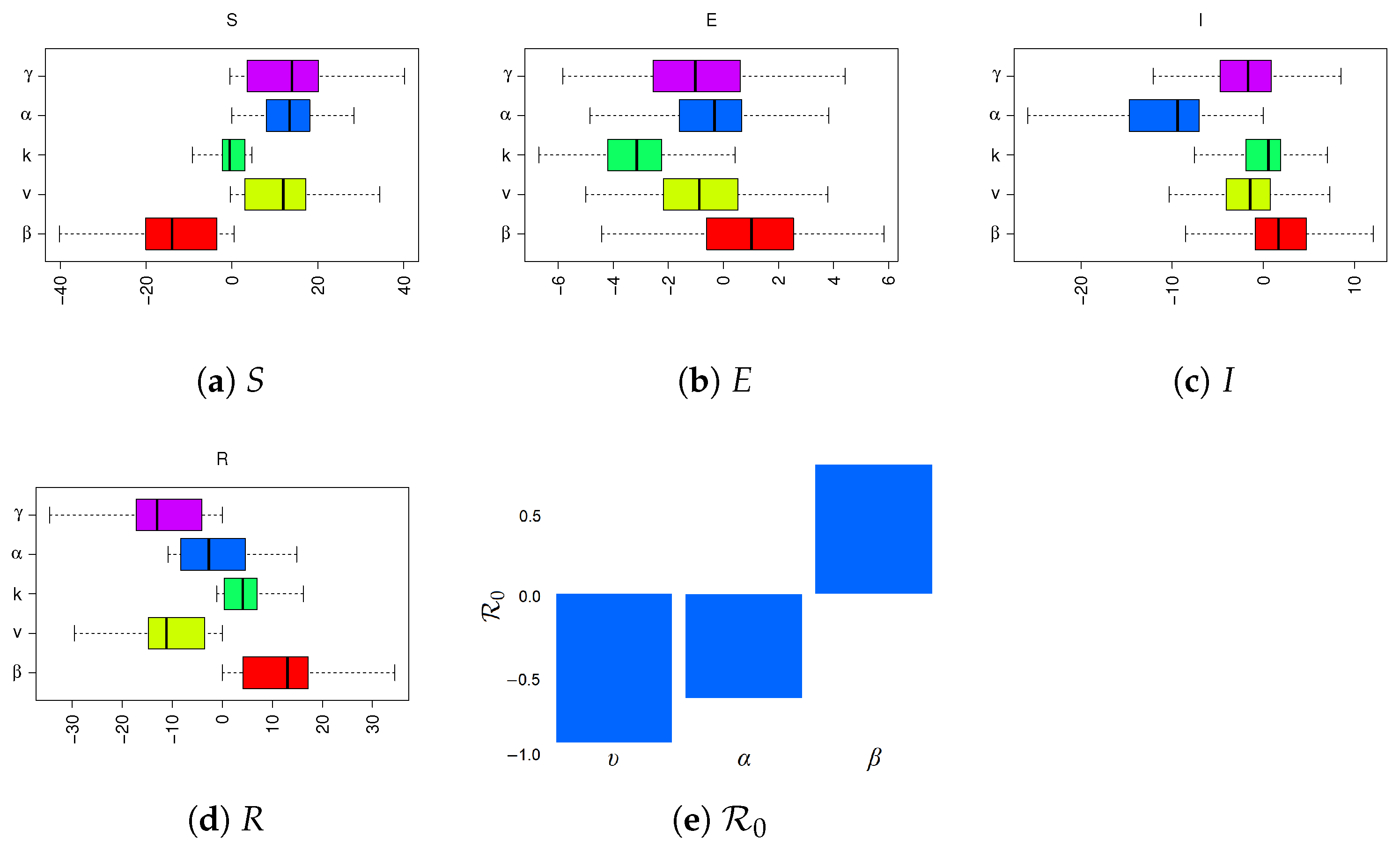
2.5. Sensitivity Analysis

We performed a sensitivity analysis of the model and ${\mathcal{R}}_0$ with respect to the parameters $\gamma ,\alpha ,k,\nu$ and $\beta$, assuming that $\nu$ is a constant parameter. We used the FME package in R for the local sensitivity analysis of variables $S,E,I,R$ and a partial rank correlation coefficient (PRCC) for ${\mathcal{R}}_0$. Results are shown in Figure 2.

The model is quite sensitive to parameters $\beta$, $\nu$, $\gamma$ and $\alpha$ and, to a lesser extent, to parameter k. This can be explained by the fact that compartment E is only a transition compartment. Indeed, modifying the value of k changes the duration spent in the exposed state and delays the infection dynamics, but does not really change the magnitude of the infection among the population. All other parameters greatly influence the dynamics; hence, a good estimation would be required in order to accurately assess the magnitude of the epidemic. This sensitivity analysis confirms that NPI intensity is a key factor for mitigating the epidemics. On the other hand, its negative influence on R means that NPIs with a higher intensity result in a lower immunity to the disease in the population.

3. Application to the COVID-19 Epidemic

Several approaches have been used to model the COVID-19 pandemic. We propose here to illustrate the model presented in the previous section with the case of COVID-19. The global response to COVID-19 is highly related to behavioral epidemiology since the only measures that were available before the appearance of the vaccine were NPIs, which consist of modifying the habits of the population. Behavioral epidemiology studies how the behavior of individuals and their lifestyle affect their health conditions and influence the dynamics of epidemics. We refer to [15] and more generally [16] as early contributions. It is obvious that the global evolution of the epidemic depends on all the decisions taken by each individual according to the context in which they finds themself and their personal situation: the age of individuals, their social status, the frequency of their daily trips to sites where the risk of infection is more or less significant, their protective behavior by using masks or even by teleworking and many other multiple aspects regarding their life style. We refer to [5] as an example for the COVID-19 epidemic taking into account different places and ages in China. We also cite a more recent contribution [17], which is a study on the influence of social cohesion and socioeconomic status on health conditions again in China.

This kind of aggregated model remains very simplistic but has the advantages of being able to be handled analytically and, more importantly, to easily exhibit major tendencies. The model that we used here is extremely simple and cannot accurately describe all the aspects of the COVID-19 pandemic. However, it is sufficient for describing the different NPI strategies and estimating at least qualitatively their effect on such a pandemic. Our choice here was to consider the individual behaviors as a single aggregated term of NPI intensity rather than considering the extreme diversity of individual behaviors, as well as a limited number of compartments. Indeed, other compartments such as quarantined, asymptomatic carriers, etc., could also be introduced and would provide a greater accuracy; however, they would only marginally modify the dynamics and would not provide much more useful information regarding the goal of this model, i.e., estimating the qualitative evolution over time of the pandemic in regard to different NPI intensity strategies.

3.1. Background of the COVID-19 Pandemic

The onset of the COVID-19 epidemic was brutal, with very high peaks of contamination leading to the saturation of intensive care units. In the United States, the occupancy rate of intensive care beds reached over $60\%$ in the most populous states and large cities [18]. In France, the number of beds able to accommodate severely ill patients requiring intensive care in hospitals was limited to around 5000 beds and the number of respirators available seemed also insufficient in view of the foreseeable arrival of seriously ill patients. In the absence of any measures, a very significant proportion of the population would have been infected after the epidemic wave. As a result, several governments in the world decided to put in place NPIs such as lockdown, social distancing or teleworking in order to limit the number of cases and keep hospital admissions of seriously ill patients below the hospital capacity threshold. This policy was adopted by many countries and worked with some success and limitations. Regardless, hospitals were under very strong pressure, sometimes leading to the saturation of intensive care units [19] despite such measures. The evaluation of the effects of NPIs is a central question that has been studied in previous works, such as [20] in Italy or in [14], where the authors evaluated how successful the governmental measures were in Rohingya refugee camps.

However, lockdown has had disastrous consequences for the economy, generating waves of unemployment and causing considerable budget deficits for the states, with very serious difficulties for those in need. Some countries have chosen to set up a partial lockdown while maintaining activity or have opted to end the lockdown early enough to limit the disastrous consequences for their economy, especially in Northern Europe. Many countries remain extremely cautious in this area, fearing the occurrence of successive epidemic waves after lockdown. The question of the end of lockdown is therefore crucial and it is important to develop scientific methods allowing us to control this phase by limiting the damage.

NPIs were set up in order to rapidly address problems such as intensive care units overload and hospital pressure. However, they were not specifically thought of as a long-term answer to a long-lasting epidemic (several years) that may be caused by reinfection. It is commonly admitted that immunity usually lasts at least six months, but there is still uncertainty about a possible loss of immunity that would happen later on. As of today, a few cases of reinfection have been reported [21]. In [22], the author spotted that reinfection is possible but the bigger question is “if reinfections are going to happen, how frequently are they happening?”. In a preprint, Ward et al. [23] observed a decline in antibodies in UK patients, which led to the fear of a possible loss of immunity. Furthermore, the appearance of new variants also increases the possibility of reinfection [24,25].

3.2. Dynamics without Protection Measures: Parameters Estimation Based on COVID-19

Much work has been devoted to modeling the COVID-19 epidemic: Refs. [26,27,28] in China, Refs. [29,30,31] in Japan and, in Algeria [32,33]. We also cite [34] in which the authors studied the effects of different quarantine and protection measures on the dynamics of the epidemic with a mathematical model, and [35] for Canada. Only a few works have been devoted to modeling the epidemic in the hypothesis of reinfection, such as [36] or [37].

The question of reinfection quickly rose with the onset of the pandemic, as it was unclear if immunity could be lost [38]. The loss of immunity or the risk of reinfection is an important question in epidemiology, such as for HIV [39]. In the context of COVID-19, few cases of re-infections have been observed [21], but most studies prior to fall 2021 suggested a long-lasting protection (≥90 days [40], ≥6 months [41]) but could not totally exclude the possibility of reinfections after a longer time or because of mutations. However, the appearance of new variants shed a light on massive reinfection occurrences. Evidence that variants could elude immune responses was found [24,25]. Several new variants (English, South African, Brazilian, Delta, Omicron) have been able to develop and even replace the original virus. These variants can be more virulent, more contagious and, for some of them, even more resistant to vaccines (see [42] for the Brazilian variant and [43] for UK and South Africa). It has recently been found that the Omicron variant might evade antibodies induced by infection or vaccination [44]. In [45], it was suggested that the relative risk of reinfection has risen to 81%. Long-term reinfections due to new variants or a loss of immunity have become a realistic hypothesis. In this general context, we considered an SEIRS model with the possibility of re-infection in the long term, with a reinfection rate $\gamma$. For the COVID-19 epidemic, we used the same general SEIRS model presented in the previous theoretical section. Since it is a highly simplified model that relies on strong assumptions, it may not be suitable for a realistic description or prediction of the current pandemic. However, it can provide useful qualitative information about the evolution of the disease in the context of possible re-infections and about the benefits and disadvantages of different NPI strategies.

Parameters of the model can be estimated from various medical and statistical reports about COVID-19.

As of 2022, though the proportion of asymptomatic carriers is pretty much well known (50% in [46], 40% in the meta-analysis performed in [47]), there is no clear consensus about the role of asymptomatic carriers on the dynamics of the population. Some studies state that more than half of infections are due to asymptomatic carriers [48], whereas other suggest that asymptomatic transmission is marginal or due to a misclassification of presymptomatic cases as asymptomatic [49,50]. Because of those uncertainties, we did not take into account separate compartments for asymptomatic and symptomatic people in this work for the sake of simplicity. Instead, we considered a class I that includes both symptomatic and presymptomatic carriers. Symptomatic carriers were included in the R class since they are supposed to be isolated as soon as they are aware of their condition. For that reason, we did not use a quarantined/isolated class as is often carried out in other approaches, such as in [51], since symptomatic/isolated and healed individuals do not play any role in the transmission of the disease. As a consequence, the average time spent in the infectious class $1/\alpha$ lies somewhere between the average infectious time for presymptomatic carriers $1/{\alpha }_p$ and the one for asymptomatic carriers $1/{\alpha }_a$, i.e., $1/\alpha \in [1/{\alpha }_p,1/{\alpha }_a]$. It was found in [52] that infectiousness can occur from 2.3 days (95% CI, 0.8–3.0 days) before symptom onset, with a peak at 0.7 days (95% CI, 0.2–2.0 days) before onset. We estimated a rough lower boundary for $1/{\alpha }_p\ge 1$. The same study found a significant decline in infectiousness 10 days after onset. Other studies suggest that an infection more than 5 days after symptoms onset is very unlikely [53]. We thus set an upper boundary for $1/{\alpha }_a\le 7.3$. As a consequence, we estimated that the parameter $\alpha$ lies in the interval $[0.13,1]$.

As a consequence, we chose to set $\alpha =0.67$ in this model. The model that we obtained does not differ qualitatively from a model with an explicit asymptomatic compartment and provides a similar dynamic, with a marginal quantitative difference. On the contrary, such an approach allows for avoiding the use of too many parameters on which there is much uncertainty, thus following the principle of parsimony. Additional information obtained by using an asymptomatic compartment would not have been useful considering the scope of our study, and it would have come with a much higher prior uncertainty.

Following the estimation of $\alpha$, we set parameter k to $0.27$ day${}^{-1}$ since the average duration between infection and symptoms onset is 5.2 days [54].

${\mathcal{R}}_0=\frac{\beta }{\alpha }$ has been estimated as between 2 and 6 for most countries, with most probable values in the range 2–3 [55]. Some other studies suggest even higher values (between 3.5 and 6 [56]). In the following simulation, we decided to set $\beta =1.2$ in order to obtain ${\mathcal{R}}_0=2.4$. In Section 5, we will estimate $\beta$ for each case study based on incidence time series obtained from data sources.

It is important to note that estimates of the previous parameters ($\alpha ,\beta ,k$) may be very inaccurate. In the case of COVID-19, one may find inconsistencies about indicators estimations between different studies: they depend on many factors (country, population density, local habits, culture, genetics), may vary in time (seasonal effects, new variants) or may be based on different protocols. Nevertheless, we sought to make a reasonable choice of parameters among those found in the literature. If there may be much uncertainty about the numerical values that we obtained from simulations, the qualitative results are robust despite the inaccuracy of the parameters estimations.

Finally, there is a major uncertainty about parameter $\gamma$ at the present time. The average duration after which immunity is lost is $1/\gamma$. Values between 60 and 365 were used in [36]. As of today, immunity is assumed to last at the very least 200 days, so we considered several possible values of $1/\gamma$ larger than 200.

Figure 3 compares several dynamics in the total absence of protective measures for a country population of 50,000,000 individuals for different values of $\gamma$. In the absence of NPI ($v=0$), the dynamics follow those of a classical SEIRS model, tending toward the endemic equilibrium with decreasing oscillations. Note that they differ from those of a classical SEIR model without reinfection ($\gamma =0$, red dashed line curve). In the latter, the epidemic eventually vanishes after one wave of infection. In addition, note that there is very little difference between the first peaks for the different values of $\gamma$.

It is known that, in the absence of any protective measure against the epidemic, a large proportion of the population is infected after the first peak in a proportion ranging from 0.8 to almost the entire population depending on the value of ${\mathcal{R}}_0$ [28,32,57]. The aim of this work was precisely to show that, by using adequate protective measures, it is possible to greatly limit the level of infection and even to cause the disappearance of the epidemic in a relatively short time.

Figure 3 shows that considering different values for $\gamma$ leads to the same qualitative dynamics. Despite the large range for $\gamma$, the amplitude of the first peak is similar, whereas the second one is shifted in time but has a similar amplitude (Figure 3a). Reinfection naturally causes an infinite growth of the cumulative cases (Figure 3b) that occurs in stages.

The number of active cases I per 100,000 at the equilibrium decreases with $1/\gamma$. However, Figure 3a illustrates that, if no control measures are taken, it remains high for a large range of values. Whatever the value of parameter $\gamma$, the first epidemic peak is very high and it is essential to take protective measures to limit the number of cases and even to stop the epidemic quickly.

4. Possible Strategies against an Epidemic with Reinfection

We now present several possible strategies to fight the epidemic when it starts. Based on the mathematical analysis of the general SEIRS model, we considered three main classes of epidemic NPI strategies: a first one consisting of a constant control, a second one stabilizing the epidemic at a sufficiently low target endemic level and a third one aiming at the eradication of the epidemic. In order to compare the various strategies, all simulations in this section used the same set of epidemiological parameters: $\beta =1.2$, $k=0.2$, $\alpha =0.5$ and $\gamma =1/200$ for a fictional disease and a fictional country with N = 50,000,000 inhabitants. All indicators (I, cumulative cases) are presented for 100,000 individuals to be consistent with indicators found in the literature.

4.1. Strategy 1: Constant Control

We compared some constant control strategies with different intensities $v_0$, shown in Figure 4. The $\widehat{v}\left(I\right)$ function is represented in red as in all the following figures.

Each intersection with a constant v function defines an endemic equilibrium, which is the case of the purple and green function. Two outcomes are possible. If $v_0$ is high enough, the epidemic goes extinct (Figure 4b) since the DFE is stable and there is no endemic equilibrium ($v=0.8$: blue and $v=0.5$: orange, Figure 4a). The number of active cases per 100,000 falls below 1 in around 80 days for $v=0.5$ and around 20 days for $v=0.8$. If $v_0$ is low, the system tends toward a stable endemic equilibrium since the DFE is unstable ($v=0.3$: purple and $v=0.2$: green). In the latter case, the number of active cases I shows oscillations and stabilizes around the endemic equilibrium. Peaks appear corresponding to different waves of infection. As $v_0$ increases, the value $I^{*}$ at the equilibrium gets lower and peaks get lower and more distant in time. The number of cumulative cases keeps increasing as people get reinfected, and its value eventually become larger than the total population.

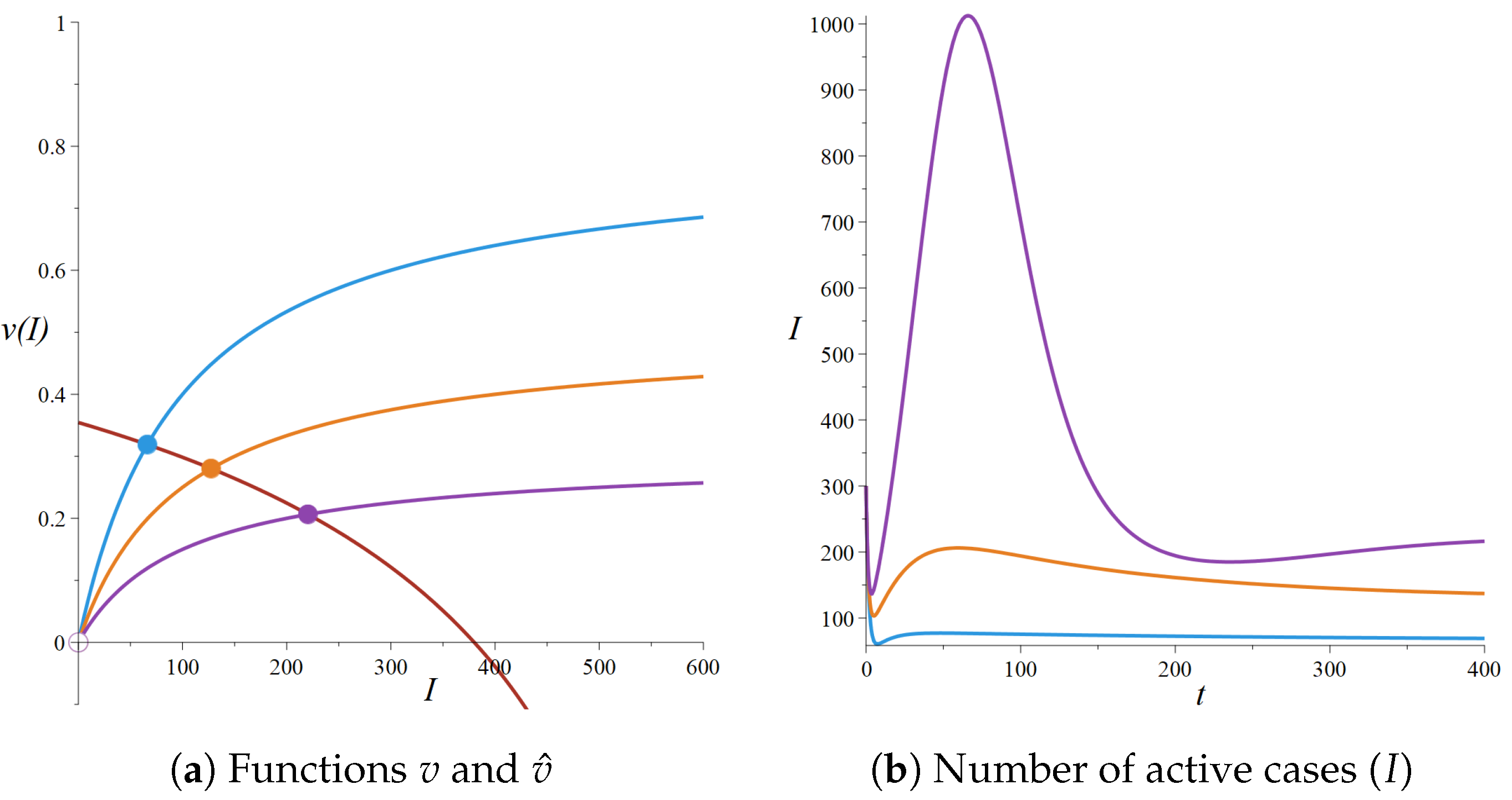
4.2. Strategy 2: NPI Intensity Increasing with the Number of Cases

This is the most natural strategy since the intensity of measures usually increases with the level of epidemics. Many governments choose to have a light level of social distancing at a low level of incidence and more effective measures at higher levels.

The dynamics present an unstable DFE and a unique endemic equilibrium. To illustrate this, we chose a family of increasing monotonic maps $v\left(I\right)$ $v:I\mapsto v_{0}I/(I+100)$ for different values of $v_0=0.8,0.5$ and 0.3 (see Figure 5). The intersection with the curve $\widehat{v}$ defines a unique endemic equilibrium $I^{*}$ that is locally asymptotically stable. The value of $I^{*}$ decreases with $v_0$: $I^{*}$ is around 220, 128 and 67 for $v_0=0.3,0.5$ and 0.8, respectively. High values of $v_0$ lead to a rapid decrease in the epidemic, whereas a low value (purple curve) still allows for large amplitude peaks that may not be manageable by hospitals.

Since the number of cases decreases with the target endemic level, this strategy may become useful for keeping the epidemic low enough to prevent hospital congestion with a lower level of active cases. Unfortunately, it is not possible to reach the extinction of the epidemic.

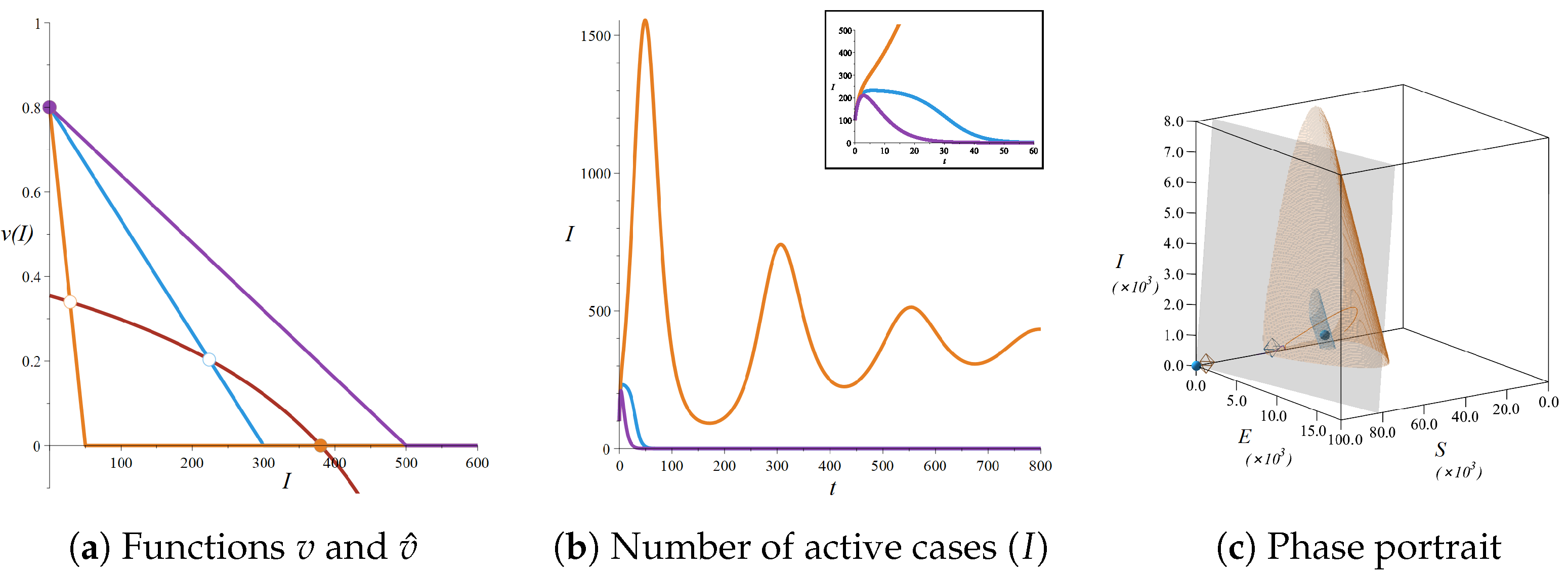
4.3. Strategy 3: Seek to Extinguish the Epidemic

A necessary condition to end the epidemic is to have a stable DFE, which requires that $v\left(0\right)>\widehat{v}\left(0\right)$. This requires a high NPI intensity at a low level of cases I, contrary to strategy 2. This can be achieved by using any function $v>\widehat{v}$, such as a sufficiently high constant control, as shown previously. A key element in our work is that, since $\widehat{v}$ is decreasing, it is much more important to keep v at high levels when I is low than when I is high. Indeed, the extinction of the epidemic can be achieved with a decreasing function, with a low-intensity NPI when I is high and a high-intensity NPI when I is low.

Figure 6 depicts the case of a decreasing control function v (purple curve). Two other control functions (orange and blue) are represented in order to see what would happen if the parameters were misevaluated. More specifically, we chose the following family of piecewise linear maps:

$$v:I\mapsto \left\{\begin{array}{cc}{v}_0\left(1-\frac{I}{I_{max}}\right)\hfill & \mathrm{if}0\le I<I_{max},\hfill \\ 0\hfill & \mathrm{if}{I}_{max}\le I.\hfill \end{array}\right.$$

(17)

with $v_0=0.8$ and $I_{max}=200$ (blue), 50 (orange) and 500 (purple) (see Figure 6a).

The purple map drives the epidemic to extinction (Figure 6b). Blue and orange maps create a lower unstable endemic equilibrium and a stable endemic equilibrium, generating an “Allee” effect: the lower the incidence, the more difficult it is for the disease can spread. Depending on the initial conditions, the epidemic may disappear or tend toward the high endemic equilibrium. The basins of attraction of the endemic equilibria for the different measures are represented in their respective colors in Figure 6c. Stronger measures lead to a smaller basin of attraction for the endemic equilibrium.

Such a strategy may be less natural since it means higher-intensity measures when I is low than when I is high. However, the intensity is still lower than in strategy 1, and it can provoke the extinction of the epidemic, which cannot be achieved with strategy 2. Furthermore, the extinction of the epidemic occurs in a relatively short time compared to the measures taken by most governments that vary in intensity and have been spread over more than a year.

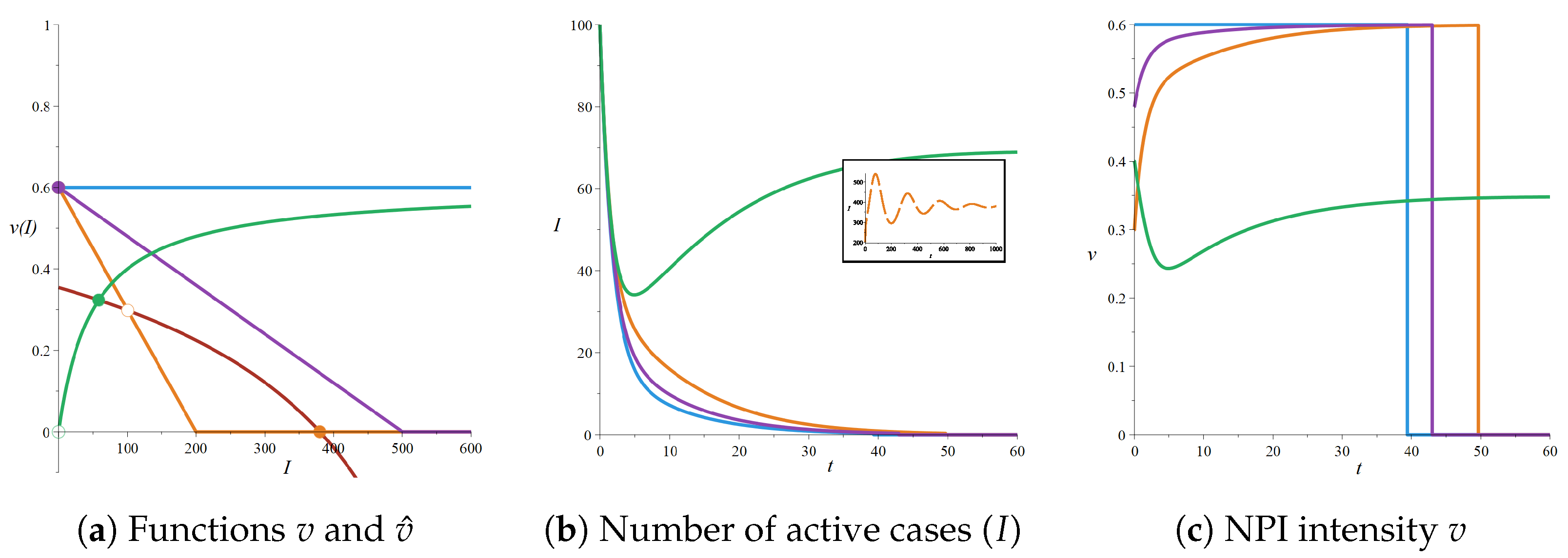
5. Case of the COVID-19 Pandemic: Estimation of NPI Intensities and Identification of the Strategies Chosen by Several Countries

We estimated the time evolution of NPI intensities $\nu \left(t\right)$ for several countries in order to find a match with one of the previous strategies discussed in the previous section. For that purpose, we used incidence (and equivalently the total number of new cases) and hospital admission (if available) data collected from John Hopkins University’s Github repository (https://github.com/CSSEGISandData/COVID-19/blob/master/csse_COVID_19_data/csse_COVID_19_time_series/, accessed on 1 March 2023) and Our World in Data (https://ourworldindata.org/COVID-vaccinations, accessed on 1 March 2023).

We simulated the evolution of the incidence using the SEIRS model defined in Section 2 with a time-varying NPI intensity $\nu \left(t\right)$. We assumed that, for each country, all parameters except $\nu \left(t\right)$ remain constant for the total duration of the simulation. For that reason, we used data time series from February 2020 to no later than October 2021 in order to avoid the effects of new variants such as delta and omicron that would make the assumption of a constant $\beta$ highly irrelevant.

Accordingly to Section 3.2, parameters $\alpha =0.67,k=0.26,\gamma =1/200$ were fixed and estimated based on medical and statistical studies. The country population was extracted from the previous sources, and parameters $\beta$ and $\nu \left(t\right)$ were fitted. Assuming that no NPI has been set up during the initial exponential phase $\nu \left(t\right)=0$, we extracted incidence data between the date with the first reported case and the end of this exponential phase (we assumed that it ends at the first inflection point, which occurs slightly before the peak maximum). We then estimated the last remaining parameter $\beta$ by fitting the incidence curve obtained from simulations with initial condition $S\left(0\right)=N,E\left(0\right)=0,I\left(0\right)=1,R\left(0\right)=0$, with the daily incidence rate provided by data from the previous sources. Using the least square method, we fitted two parameters $\beta$ and the fictional start date $t_0$ (theoretical date at which $I\left(t_0\right)=1$).

We then assumed that, after this initial exponential phase, the infection rate $\beta$ remains constant, but, since NPIs have been set up, $\nu \left(t\right)$ now evolves with time. For the sake of simplicity, we considered that the NPI intensity $\nu \left(t\right)$ is the same for all the days of a same week. We fitted $\nu \left(t\right)$ with the least square method since the number of values of $\nu \left(t\right)$ is still large (1 per week), and we used a hill climbing algorithm in order to find the best fit. Finally, we smoothed the results by taking the mean over 7 days.

We then intended to identify the strategies used by comparing the values of $\nu$ with the incidence and tried to exhibit a tendency. Since the incidence may be underestimated during the first wave of the epidemic, we also compared $\nu$ to the number of admissions in hospitals (when data are available), which is supposed to be a scaled and slightly shifted version of the real incidence curve. It then may provide a more reliable estimation of the real incidence rate up to a multiplicative constant. Moreover, NPIs were often set in order to avoid hospitals and ICUs saturation, which also makes this indicator more relevant than the observed incidence. Figure 7 shows the results obtained for the United Kingdom, France, Germany and New York City. This figure shows the time evolution of new cases, hospitalizations and $\nu \left(t\right)$, as well as the phase portraits $\nu$ vs. new cases and $\nu$ vs. hospitalizations. Results for a few other countries are shown in Appendix C, Figure A2. Note that we replaced the incidence rate by the number of new cases, which is just a scaled version that is of the same order as the hospitalization number, which makes the figure easier to read.

It appears that the NPI intensity is not highly linearly correlated to new cases or hospitalization, apart from France ($R^2=0.40$), which could be associated to strategy 2. For other countries, the value of $\nu$ appears to be relatively constant or slightly increasing with the new cases or hospitalizations; hence, they can be associated to strategy 1 or 2. An increase in the NPI intensity around the incidence peaks on the time series confirms that the chosen strategy is more likely to be strategy 2. Other countries shown in the appendix exhibit a constant or slightly increasing tendency, except for Russia, which exhibits a slightly decreasing tendency, which can be considered as constant. For the United Kingdom, $\nu$ seems to slightly decrease with the number of cases, but is constant with hospitalizations, which certainly illustrates that hospitalization works better than the measured incidence rate. All those examples illustrate that strategies 1 and 2 appear to be more natural than strategy 3, and thus are chosen by most countries.

We compared those strategies with the ones chosen by two countries that allegedly maintained a very low incidence: New Zealand and Vietnam. New Zealand adopted an elimination strategy in response to COVID-19 (“keep it out, prepare for it, stamp it out”) after an initial lockdown from 25 March 2020,which was progressively lifted after 28 April 2020. It included a strong border control of the island, contact tracing and strong public measures. As a continental country, Vietnam imposed a strict border control with a long quarantine for travelers, as well as very localized and strong lockdowns. Both countries experienced a very low incidence level and maintained relatively normal activity at the moment when other countries were struck by incidence peaks (winter 2020–2021). Incidence and NPI intensity are shown for both countries in Figure 8 (no hospitalization data were available from the previous sources).

The NPI intensity seems to be constant or decreasing with the incidence rate, with the highest values reached at very low incidence rates. Incidence peaks do not seem to be associated with stronger measures but are more constant in intensity. For those reasons, our estimation of NPI intensity for those countries seem to be consistent with strategy 3.

6. Comparison and Discussion of the Effects of Various NPI Strategies on the Dynamics of the Epidemic

We have shown that we can control an epidemic when it starts by imposing a level of NPI that depends on the number of infected persons each day. In the absence of protective measures, a peak of infected cases reaches over 6000 cases per 100,000 and lasts for around 150 days. We now compare the different strategies used to control the epidemic: strategies 1 (blue), 2 (green) and 3 (purple and orange); see Figure 9a. All strategies have the same maximum intensity $v_0=0.6$. Blue and purple always cause the epidemic to end since the only equilibrium is the DFE. The green strategy leads to a low endemic equilibrium. The orange strategy leads either to an endemic equilibrium or to the extinction of the epidemic depending on the initial condition (Figure 9b).

The benefit of the orange strategy over the purple one is its lower intensity. This comes along with the risk of the dynamics ending trapped at the endemic equilibrium if the initial condition is unfavorable, i.e., when NPIs are set up too late (insert of Figure 9b).

We set a threshold (here, less than 1 case per 100,000) under which we consider that the epidemic has gone extinct. When the number of cases falls under this threshold, we assume that it is not necessary to maintain any NPI. The duration and the time evolution of NPI intensity is represented in Figure 9c. The green strategy keeps the epidemic at a low level; it requires a moderately intense but never-ending NPI. Strategy 1 (blue, constant $v=0.6$) is the most effective and has the shortest total NPI duration but may be difficult to implement from the start. It drives the epidemic to extinction in 39 days. It should be noticed that $0.6$ already represents a high-intensity NPI, such as a lockdown, that may be difficult to set up in practice or that at least requires some time to be achieved. For the same initial condition, NPIs for purple and orange strategies last 43 and 49 days, respectively. They have the advantage of proposing NPIs with a gradually increasing intensity that reaches the maximum value at the end of the epidemic, which gives health authorities more time to set it up. Overall, their duration seems reasonable compared to the one of the blue strategy.

The analysis of the dynamics of the epidemic for those different strategies allows us to rank their effectiveness, intensity and duration, as shown in

Table 2. Comparison of the effectiveness, intensity and duration for the different strategies, for the same maximum intensity.

	Strategy 1	Strategy 2	Strategy 3
Effectiveness	high	low	high
Intensity	highest	medium	high
Duration	short	very long	short

.

The effectiveness is clearly higher in strategies 1 and 3 than in 2 since the latter is unable to prevent the endemic equilibrium and put an end to the epidemic by itself. Type 2 strategies do not seem desirable to us because they lead to a permanent endemic state with lasting NPI measures, even if they may allow for limiting the magnitude of an epidemic peak in order to prevent ICU saturation. Strategy 3 combines the advantages of efficiency, a shorter duration and a lower intensity than strategy 1. Based on those findings, it seems more profitable to seek to get rid of the epidemic using a purple or orange strategy (strategy 3). However, it may seem counter-intuitive in the sense that it is necessary to strengthen the NPI intensity as the number of infected persons decreases in order to achieve the eradication of the epidemic in some time frame.

Those strategies have different outcomes in terms of social and economic costs. Strategies 1 and 3 have a short duration but a high intensity, contrary to strategy 2, which has a very long duration and a moderate intensity. NPIs are known to induce much stress and anxiety and, more generally, a decline in mental health [58,59]. We do not discuss this matter here, but there is a need to carefully consider a possible trade-off between the duration and intensity of NPIs.

As shown in the previous section, most countries have adopted strategy 1 (blue) or 2 (green) instead, except for New Zealand and Vietnam. When the health situation worsens, the level of measures is reinforced for some weeks in order to return to a lower level of virus circulation, resulting in successive epidemic waves. In France, three lockdowns have been established. For each lockdown, its intensity has been reduced when the epidemic peak has diminished sufficiently so as not to saturate the hospitals but without maintaining it long enough at a high level to bring about the eradication of the epidemic. These successive confinements have generated astronomical infections and economic costs. Epidemic waves seem to endlessly follow each other unless a vaccination policy can achieve collective immunity. On the contrary, New Zealand and Vietnam maintained a low incidence level and seem to have suffered a lower social and economic cost, except for tourism.

To summarize, our results indicate that lockdowns should be strengthened and absolutely not released when the incidence drops until the epidemic actually ends. Carrying out the contrary leads to a new increase in the number of cases toward an endemic equilibrium.

In our opinion, these epidemic control methods could be used locally for medium-sized cities that can be isolated for a period of at least one to two months by prohibiting or very strictly controlling the entry and exit of people from this city. The application of these classes of strategies would require the use of a significant number of tests allowing for a good estimation of the numbers of infected people at the time when the control must be implemented. It requires properly positioning the various endemic equilibria created by the epidemic control function. In the context of COVID-19, our work suggests that strong, short and early measures are more effective than mild but long-lasting ones. We think that these results may be of interest since some countries such as Israel expect to live permanently with the disease.

7. Conclusions

In this work, we studied an SEIRS epidemic model with reinfection and illustrated the results with an application to the COVID-19 pandemic. We analyzed the effects of several kinds of infection-dependent NPIs on the dynamics of the epidemic and on the characteristics (existence and stability) of disease-free and endemic equilibria. We showed that NPI strategies could be divided into three main classes and highlighted their benefits and drawbacks, such as their ability to put an end to the epidemic, the amplitude and duration of the peaks and the feasibility of the considered measures. We found that constant NPI strategies are effective for extinguishing the epidemic but may be too intense to be practically usable. Strategies with NPI intensity decreasing with the number of cases I may also put an end to the epidemic by creating an Allee effect while being easier to set up. However, they can lead to a large epidemic peak or a (lower) endemic equilibrium instead of extinction if they are not set up carefully. Finally, the most intuitive strategy (NPI intensity increasing with the number of cases) proved to be the least efficient while being unable to put an end to the epidemic.

The key element of our study is that, in the context of the spread of a disease with a loss of immunity, Allee effects do not exist naturally, contrary to what is observed in population ecology. However, while this phenomenon is not desirable in the latter, it appears to be mandatory to end an epidemic, and has to be artificially created using NPIs. In terms of public health, creating an Allee effect would imply setting up early measures with more intensity. Strategies such as type 3 can bring about the extinction of the epidemic and could have important implications for public health policy. They are already in use for animal epidemics: in the case of diseases spreading in farms animals, the decision is often to kill all the animals in a same location. Such policies prevent the disease from spreading at a larger scale but are highly controversial. The situation seems more delicate in the case of human epidemics because even softer policies such as travel restrictions and confinement measures are difficult to impose. However, a more systematic and efficient screening, better information and very localized and short lockdowns may prevent major outbreaks. Many countries decided to use strategies 1 or 2 against COVID-19, as we showed in Section 5, and failed to create an Allee effect. They have been reluctant to set high-intensity NPIs at low virus circulation levels or during the early stages of the pandemic because carrying this out may have been greatly unpopular and a major restriction of liberties, but possibly also because of the financial cost. However, our work suggests that spending money for early prevention, information and screening may reduce the final cost. Even if our results may be considered with care due to the many assumptions that we made in our model, we think that we have provided a good illustration that (1) delaying the response to a problem eventually results in a highest social and economical cost, and (2) people are nevertheless inclined to use that kind of sub-efficient strategy. We believe that such a conclusion holds for other major problems that we are facing nowadays, particularly for the ones related to climate change. We illustrated our model with the case of COVID-19. However, further investigations on other epidemics would be necessary to identify what strategies are commonly used and to confirm if strategy 3 is the most efficient.

As a perspective, we could study a network of several cities connected by the movement of individuals from one city to another by rail or by plane. It would be interesting to study the coupling of epidemic management methods depending on the number of infected people in the different cities. We refer to [60,61] for disease spread in meta-populations.

In the future, we plan to reconsider our model by considering two compartments for asymptomatic (A) and infectious (I) carriers in a future SEAIRS version. We also plan to improve the realism of the model by explicitly including other factors, such as vaccination, health infrastructures and a more detailed description of social behaviors. We also plan to provide a more detailed study on the economic and social costs of NPIs. However, we hope and are inclined to think that our conclusions obtained through a theoretical approach on the effectiveness of the various strategies can be useful for practical case studies, as density-dependent protection strategies could be used to target a sufficiently low level of endemicity or find a strategy to put an end to the epidemic while considering constraints such as social cost or hospitals capacity.

References

1. Allee, W.C.; Bowen, E.S. Studies in animal aggregations: Mass protection against colloidal silver among goldfishes. J. Exp. Zool. 1932, 61, 185–207. [Google Scholar] [CrossRef]
2. Odum, E.P.; Barrett, G.W. Fundamentals of Ecology; Saunders Philadelphia: Philadelphia, PA, USA, 1971. [Google Scholar]
3. Courchamp, F.; Berec, L.; Gascoigne, J. Allee Effects in Ecology and Conservation; OUP Oxford: Singapore, 2008. [Google Scholar]
4. Holden, M.H.; McDonald-Madden, E. High prices for rare species can drive large populations extinct: The anthropogenic Allee effect revisited. J. Theor. Biol. 2017, 429, 170–180. [Google Scholar] [CrossRef] [PubMed] [Green Version]
5. Liu, Y.; Gu, Z.; Xia, S.; Shi, B.; Zhou, X.N.; Shi, Y.; Liu, J. What are the underlying transmission patterns of COVID-19 outbreak? An age-specific social contact characterization. EClinicalMedicine 2020, 22, 100354. [Google Scholar] [CrossRef]
6. Xia, S.; Liu, J.; Cheung, W. Identifying the relative priorities of subpopulations for containing infectious disease spread. PLoS ONE 2013, 8, e65271. [Google Scholar] [CrossRef] [PubMed] [Green Version]
7. Perkins, T.A.; Paz-Soldan, V.A.; Stoddard, S.T.; Morrison, A.C.; Forshey, B.M.; Long, K.C.; Halsey, E.S.; Kochel, T.J.; Elder, J.P.; Kitron, U.; et al. Calling in sick: Impacts of fever on intra-urban human mobility. Proc. R. Soc. B Biol. Sci. 2016, 283, 20160390. [Google Scholar] [CrossRef] [PubMed] [Green Version]
8. Auger, P.; Moussaoui, A. On the Threshold of Release of Confinement in an Epidemic SEIR Model Taking into Account the Protective Effect of Mask. Bull. Math. Biol. 2021, 83, 25. [Google Scholar] [CrossRef] [PubMed]
9. Howard, J.; Huang, A.; Li, Z.; Tufekci, Z.; Zdimal, V.; van der Westhuizen, H.M.; von Delft, A.; Price, A.; Fridman, L.; Tang, L.H.; et al. An evidence review of face masks against COVID-19. Proc. Natl. Acad. Sci. USA 2021, 118, e2014564118. [Google Scholar] [CrossRef] [PubMed]
10. van den Driessche, P.; Watmough, J. Reproduction numbers and sub-threshold endemic equilibria for compartmental models of disease transmission. Math. Biosci. 2002, 180, 29–48. [Google Scholar] [CrossRef]
11. Fehlberg, E. Klassische Runge-Kutta-Formeln vierter und niedrigerer Ordnung mit Schrittweiten-Kontrolle und ihre Anwendung auf Wärmeleitungsprobleme. Computing 1970, 6, 61–71. [Google Scholar] [CrossRef]
12. Shokri, A.; Mehdizadeh Khalsaraei, M.; Molayi, M. Nonstandard Dynamically Consistent Numerical Methods for MSEIR Model. J. Appl. Comput. Mech. 2022, 8, 196–205. [Google Scholar] [CrossRef]
13. Khalsaraei, M.M.; Shokri, A.; Ramos, H.; Heydari, S. A positive and elementary stable nonstandard explicit scheme for a mathematical model of the influenza disease. Math. Comput. Simul. 2021, 182, 397–410. [Google Scholar] [CrossRef]
14. Kamrujjaman, M.; Mahmud, M.S.; Ahmed, S.; Qayum, M.O.; Alam, M.M.; Hassan, M.N.; Islam, M.R.; Nipa, K.F.; Bulut, U. SARS-CoV-2 and Rohingya Refugee Camp, Bangladesh: Uncertainty and How the Government Took Over the Situation. Biology 2021, 10, 124. [Google Scholar] [CrossRef] [PubMed]
15. Bauch, C.; d’Onofrio, A.; Manfredi, P. Behavioral Epidemiology of Infectious Diseases: An Overview. In Modeling the Interplay between Human Behavior and the Spread of Infectious Diseases; Springer Science & Business Media: Berlin/Heidelberg, Germany, 2012; pp. 1–19. [Google Scholar] [CrossRef]
16. Manfredi, P.; D’Onofrio, A. Modeling the Interplay between Human Behavior and the Spread of Infectious Diseases; Springer: New York, NY, USA, 2013. [Google Scholar] [CrossRef]
17. Feng, Z.; Cramm, J.M.; Nieboer, A.P. Associations of Social Cohesion and Socioeconomic Status with Health Behaviours among Middle-Aged and Older Chinese People. Int. J. Environ. Res. Public Health 2021, 18, 4894. [Google Scholar] [CrossRef]
18. Centers for Disease Control. 2021. Available online: https://www.cdc.gov/nhsn/covid19/report-patient-impact.html (accessed on 1 March 2023).
19. Trentini, F.; Marziano, V.; Guzzetta, G.; Tirani, M.; Cereda, D.; Poletti, P.; Piccarreta, R.; Barone, A.; Preziosi, G.; Arduini, F.; et al. Pressure on the Health-Care System and Intensive Care Utilization During the COVID-19 Outbreak in the Lombardy Region of Italy: A Retrospective Observational Study in 43,538 Hospitalized Patients. Am. J. Epidemiol. 2021, 191, 137–146. [Google Scholar] [CrossRef] [PubMed]
20. Antonini, C.; Calandrini, S.; Stracci, F.; Dario, C.; Bianconi, F. Mathematical Modeling and Robustness Analysis to Unravel COVID-19 Transmission Dynamics: The Italy Case. Biology 2020, 9, 394. [Google Scholar] [CrossRef]
21. Ota, M. Will we see protection or reinfection in COVID-19? Nat. Rev. Immunol. 2020, 20, 351. [Google Scholar] [CrossRef]
22. Stokel-Walker, C. What we know about COVID-19 reinfection so far. BMJ 2021, 372, n99. [Google Scholar] [CrossRef]
23. Ward, H.; Cooke, G.; Atchison, C.; Whitaker, M.; Elliott, J.; Moshe, M.; Brown, J.C.; Flower, B.; Daunt, A.; Ainslie, K.; et al. Declining prevalence of antibody positivity to SARS-CoV-2: A community study of 365,000 adults. Lancet Reg. Health-Eur. 2021, 4, 100098. [Google Scholar] [CrossRef]
24. Callaway, E. Fast-spreading COVID variant can elude immune responses. Nature 2021, 589, 500–501. [Google Scholar] [CrossRef]
25. Tillett, R.L.; Sevinsky, J.R.; Hartley, P.D.; Kerwin, H.; Crawford, N.; Gorzalski, A.; Laverdure, C.; Verma, S.C.; Rossetto, C.C.; Jackson, D.; et al. Genomic evidence for reinfection with SARS-CoV-2: A case study. Lancet Infect. Dis. 2021, 21, 52–58. [Google Scholar] [CrossRef]
26. Adam, D. MODELLING THE PANDEMIC The simulations driving the world’s response to COVID-19. Nature 2020, 580, 316–318. [Google Scholar] [CrossRef] [PubMed] [Green Version]
27. Kissler, S.M.; Tedijanto, C.; Goldstein, E.; Grad, Y.H.; Lipsitch, M. Projecting the transmission dynamics of SARS-CoV-2 through the postpandemic period. Science 2020, 368, 860–868. [Google Scholar] [CrossRef] [PubMed]
28. Bacaër, N. Un modèle mathématique des débuts de l’épidémie de coronavirus en France. Math. Model. Nat. Phenom. 2020, 15, 29. [Google Scholar] [CrossRef]
29. Liu, Z.; Magal, P.; Seydi, O.; Webb, G. Understanding unreported cases in the COVID-19 epidemic outbreak in Wuhan, China, and the importance of major public health interventions. Biology 2020, 9, 50. [Google Scholar] [CrossRef] [Green Version]
30. Sun, H.; Qiu, Y.; Yan, H.; Huang, Y.; Zhu, Y.; Gu, J.; Chen, S.X. Tracking Reproductivity of COVID-19 Epidemic in China with Varying Coefficient SIR Model. J. Data Sci. 2022, 18, 455–472. [Google Scholar] [CrossRef]
31. Kuniya, T. Prediction of the epidemic peak of coronavirus disease in Japan, 2020. J. Clin. Med. 2020, 9, 789. [Google Scholar] [CrossRef] [Green Version]
32. Moussaoui, A.; Auger, P. Prediction of confinement effects on the number of COVID-19 outbreak in Algeria. Math. Model. Nat. Phenom. 2020, 15, 37. [Google Scholar] [CrossRef]
33. Moussaoui, A.; Zerga, E.H. Transmission dynamics of COVID-19 in Algeria: The impact of physical distancing and face masks. Aims Public Health 2020, 7, 816. [Google Scholar] [CrossRef]
34. Kucharski, A.J.; Klepac, P.; Conlan, A.J.; Kissler, S.M.; Tang, M.L.; Fry, H.; Gog, J.R.; Edmunds, W.J.; Emery, J.C.; Medley, G.; et al. Effectiveness of isolation, testing, contact tracing, and physical distancing on reducing transmission of SARS-CoV-2 in different settings: A mathematical modelling study. Lancet Infect. Dis. 2020, 20, 1151–1160. [Google Scholar] [CrossRef]
35. Tuite, A.R.; Fisman, D.N.; Greer, A.L. Mathematical modelling of COVID-19 transmission and mitigation strategies in the population of Ontario, Canada. Cmaj 2020, 192, E497–E505. [Google Scholar] [CrossRef] [Green Version]
36. Malkov, E. Simulation of coronavirus disease 2019 (COVID-19) scenarios with possibility of reinfection. Chaos Solitons Fractals 2020, 139, 110296. [Google Scholar] [CrossRef]
37. Batistela, C.M.; Correa, D.P.; Bueno, Á.M.; Piqueira, J.R.C. SIRSi compartmental model for COVID-19 pandemic with immunity loss. Chaos Solitons Fractals 2021, 142, 110388. [Google Scholar] [CrossRef]
38. Costa, A.O.C.; de Carvalho Aragão Neto, H.; Lopes Nunes, A.P.; Dias de Castro, R.; Nóbrega de Almeida, R. COVID-19: Is reinfection possible? EXCLI J. 2021, 20, 522–536. [Google Scholar] [CrossRef]
39. Cai, L.; Liu, J.; Chen, Y. Dynamics of an Age-Structured HIV Model with Super-Infection. Appl. Comput. Math. Int. J. 2021, 20, 257–276. [Google Scholar]
40. Sheehan, M.M.; Reddy, A.J.; Rothberg, M.B. Reinfection Rates Among Patients Who Previously Tested Positive for Coronavirus Disease 2019: A Retrospective Cohort Study. Clin. Infect. Dis. Off. Publ. Infect. Dis. Soc. Am. 2021, 73, 1882–1886. [Google Scholar] [CrossRef] [PubMed]
41. Hanrath, A.T.; Payne, B.A.I.; Duncan, C.J.A. Prior SARS-CoV-2 infection is associated with protection against symptomatic reinfection. J. Infect. 2021, 82, e29–e30. [Google Scholar] [CrossRef] [PubMed]
42. Sabino, E.C.E.A. Resurgence of COVID-19 in Manaus, Brazil, despite high seroprevalence. Lancet 2021, 397, 452–455. [Google Scholar] [CrossRef]
43. Goddard, A.F.; Patel, M. SARS-CoV-2 variants and ending the COVID-19 pandemic. Lancet 2021, 397, 952–954. [Google Scholar]
44. Hoffmann, M.; Krüger, N.; Schulz, S.; Cossmann, A.; Rocha, C.; Kempf, A.; Nehlmeier, I.; Graichen, L.; Moldenhauer, A.S.; Winkler, M.S.; et al. The Omicron variant is highly resistant against antibody-mediated neutralization: Implications for control of the COVID-19 pandemic. Cell 2022, 185, 447–456.e11. [Google Scholar] [CrossRef] [PubMed]
45. Ferguson, N. Report 49: Growth and Immune Escape of the Omicron SARS-CoV-2 Variant of Concern in England; Technical Report; Imperial College London: London, UK, 2021. [Google Scholar] [CrossRef]
46. Santé Publique France. 2021. Available online: https://www.santepubliquefrance.fr/dossiers/coronavirus-covid-19/coronavirus-chiffres-cles-et-evolution-de-\la-covid-19-en-france-et-dans-le-monde/articles/covid-19-tableau-de-bord\-del-epidemie-en-chiffres (accessed on 26 October 2022).
47. Ma, Q.; Liu, J.; Liu, Q.; Kang, L.; Liu, R.; Jing, W.; Wu, Y.; Liu, M. Global Percentage of Asymptomatic SARS-CoV-2 Infections Among the Tested Population and Individuals With Confirmed COVID-19 Diagnosis: A Systematic Review and Meta-analysis. JAMA Netw. Open 2021, 4, e2137257. [Google Scholar] [CrossRef]
48. Johansson, M.A.; Quandelacy, T.M.; Kada, S.; Prasad, P.V.; Steele, M.; Brooks, J.T.; Slayton, R.B.; Biggerstaff, M.; Butler, J.C. SARS-CoV-2 Transmission From People Without COVID-19 Symptoms. JAMA Netw. Open 2021, 4, e2035057. [Google Scholar] [CrossRef]
49. Bender, J.K.; Brandl, M.; Höhle, M.; Buchholz, U.; Zeitlmann, N. Analysis of Asymptomatic and Presymptomatic Transmission in SARS-CoV-2 Outbreak, Germany, 2020. Emerg. Infect. Dis. 2021, 27, 1159–1163. [Google Scholar] [CrossRef]
50. Luo, L.; Liu, D.; Liao, X.; Wu, X.; Jing, Q.; Zheng, J.; Liu, F.; Yang, S.; Bi, H.; Li, Z.; et al. Contact settings and risk for transmission in 3410 close contacts of patients with COVID-19 in Guangzhou, China: A prospective cohort study. Ann. Intern. Med. 2020, 173, 879–887. [Google Scholar] [CrossRef]
51. Martcheva, M. An Introduction to Mathematical Epidemiology; Volume 61: Texts in Applied Mathematics; Springer: Boston, MA, USA, 2015. [Google Scholar] [CrossRef]
52. He, X.; Lau, E.H.; Wu, P.; Deng, X.; Wang, J.; Hao, X.; Lau, Y.C.; Wong, J.Y.; Guan, Y.; Tan, X.; et al. Temporal dynamics in viral shedding and transmissibility of COVID-19. Nat. Med. 2020, 26, 672–675. [Google Scholar] [CrossRef] [Green Version]
53. Walsh, K.A.; Spillane, S.; Comber, L.; Cardwell, K.; Harrington, P.; Connell, J.; Teljeur, C.; Broderick, N.; Gascun, C.F.D.; Smith, S.M.; et al. The duration of infectiousness of individuals infected with SARS-CoV-2. J. Infect. 2020, 81, 847–856. [Google Scholar] [CrossRef] [PubMed]
54. Lauer, S.A.; Grantz, K.H.; Bi, Q.; Jones, F.K.; Zheng, Q.; Meredith, H.R.; Azman, A.S.; Reich, N.G.; Lessler, J. The incubation period of coronavirus disease 2019 (COVID-19) from publicly reported confirmed cases: Estimation and application. Ann. Intern. Med. 2020, 172, 577–582. [Google Scholar] [CrossRef] [Green Version]
55. Hilton, J.; Keeling, M.J. Estimation of country-level basic reproductive ratios for novel Coronavirus (SARS-CoV-2/COVID-19) using synthetic contact matrices. PLoS Comput. Biol. 2020, 16, e1008031. [Google Scholar] [CrossRef] [PubMed]
56. Ke, R.; Romero-Severson, E.; Sanche, S.; Hengartner, N. Estimating the reproductive number R0 of SARS-CoV-2 in the United States and eight European countries and implications for vaccination. J. Theor. Biol. 2021, 517, 110621. [Google Scholar] [CrossRef] [PubMed]
57. Ferguson, N.M.; Laydon, D.; Nedjati-Gilani, G.; Imai, N.; Ainslie, K.; Baguelin, M.; Bhatia, S.; Boonyasiri, A.; Cucunubá, Z.; Cuomo-Dannenburg, G.; et al. Impact of non-pharmaceutical interventions (NPIs) to reduce COVID-19 mortality and healthcare demand. Imperial College COVID-19 Response Team. Imp. Coll. COVID-19 Response Team 2020, 20, 77482. [Google Scholar]
58. Hoffart, A.; Johnson, S.U.; Ebrahimi, O.V. Loneliness and Social Distancing During the COVID-19 Pandemic: Risk Factors and Associations With Psychopathology. Front. Psychiatry 2020, 11, 589127. [Google Scholar] [CrossRef]
59. Lüdecke, D.; von dem Knesebeck, O. Decline in Mental Health in the Beginning of the COVID-19 Outbreak Among European Older Adults—Associations With Social Factors, Infection Rates, and Government Response. Front. Public Health 2022, 10, 844560. [Google Scholar] [CrossRef] [PubMed]
60. Arino, J.; Van Den Driessche, P. The basic reproduction number in a multi-city compartmental epidemic model. In Positive Systems; Springer: Berlin/Heidelberg, Germany, 2003; pp. 135–142. [Google Scholar]
61. Arino, J.; Van den Driessche, P. Disease spread in metapopulations. Fields Inst. Commun. 2006, 48, 1–13. [Google Scholar]
Figure 1. Reduction in the number of infections due to NPI. Infected individuals are represented in blue, and symptomatic/presymptomatic in orange. Infections are represented by a gray arrow. Red crosses signal the infections that do not occur anymore due to NPI. (a) Without NPI, four infections occur. (b) With NPI, a proportion v = 0.5 of individuals are isolated (shaded area). The number of infections is reduced to ( 1 v ) 2 = 0.25 of the number of original number of infections.
Mathematics 11 02822 g001
Figure 2. Sensitivity analysis for (a) S, (b) E, (c) I, (d) R and (e) R 0 , taking into account parameters γ (purple), α (blue), k (green), ν (yellow) and β (red). Parameters values are β = 1.2 , k = 0.2 , α = 0.5 , v = 0.4 and γ = 1 / 200 , N = 100 .
Mathematics 11 02822 g002
Figure 3. Evolution of the epidemic in the absence of NPI v = 0 for 1 / γ = 200 (blue), 400 (green) and compared to a model without reinfection ( γ = 0 , red dashed curve). (a) Active cases per 100,000 (b) and cumulative cases per 100,000. The initial conditions are ( S ( 0 ) = N 1 , E ( 0 ) = 0 , I ( 0 ) = 1 ) . Parameters values are β = 1.2 , k = 0.27 , α = 0.67 and N = 50,000,000.
Mathematics 11 02822 g003
Figure 4. Comparison of constant control strategies: v = 0.8 (blue), v = 0.5 (orange), v = 0.3 (purple), v = 0.2 (green). Parameters values are β = 1.2 , k = 0.2 , α = 0.5 and γ = 1 / 200 , N = 50,000,000. The initial condition is I(0) = 300 per 100,000. (a) Comparison of functions v and v ^ (red curve) with stable (solid circles) and unstable (empty circles) equilibria. (b) Evolution of the number of active cases I. An insert shows the details of the region 0 < t < 50 . (c) Evolution of the number of cumulative cases.
Mathematics 11 02822 g004
Figure 5. Comparison of strategies lowering the endemic equilibrium. Chosen functions are v : I v 0 I / ( I + 100 ) , with v 0 = 0.8 (blue), v 0 = 0.5 (orange) and v 0 = 0.3 (purple). Parameters values are β = 1.2 , k = 0.2 , α = 0.5 and γ = 1 / 200 . The initial condition is I(0) = 300 per 100,000 individuals. (a) Comparison of functions v and v ^ (red curve) with stable endemic equilibria (solid circles) and an unstable DFE (empty circle). (b) Evolution of the number of active cases I per 100,000 individuals.
Mathematics 11 02822 g005
Figure 6. Comparison of control strategies that create an Allee effect. Chosen functions are piecewise linear maps, decreasing from 0.8 to 0 from I = 0 to I = I m a x and equal to 0 elsewhere, with I m a x = 300 (blue), I m a x = 50 (orange) and I m a x = 500 (purple). Parameters values are β = 1.2 , k = 0.2 , α = 0.5 and γ = 1 / 200 for a population of 50,000,000 individuals. The initial conditions are S0 = 60,000, E 0 = 800 , I 0 = 100 for 100,000 individuals. (a) Comparison of functions v and v ^ (red curve) with a stable (solid circle) DFE and unstable (empty circles) endemic equilibria. (b) Evolution of the number of active cases I. The early dynamics are depicted in insert. (c) Phase portrait. Stable equilibria are represented by a solid sphere, and unstable equilibria by a diamond, in colors corresponding to their respective maps v. Surfaces indicate the basin of attractions of the stable endemic equilibrium, the colors corresponding to their respective maps. The gray plane delimits the volume of possible initial conditions ( S + E + I + R N ).
Mathematics 11 02822 g006
Figure 7. Epidemiological dynamics and NPI strategies for UK, France, Germany and New York City. Left: time evolution of the number of new cases, admission to hospitals and NPI intensity ν . Middle: phase portrait of NPI intensity ν vs. new cases. Right: phase portrait of NPI intensity ν vs. hospitalizations. For each point cloud, linear regression was performed in order to see if a linear relationship could be exhibited.
Mathematics 11 02822 g007
Figure 8. Epidemiological dynamics and NPI strategies for New Zealand and Vietnam. Left: time evolution of the number of new cases (blue) and NPI intensity (grey) ν . Right: phase portrait of NPI intensity ν vs. new cases and linear regression.
Mathematics 11 02822 g008
Figure 9. Comparison of the different NPI strategies: constant control (blue), decreasing function (purple and orange) and lower endemic equilibrium (green). Parameters values are β = 1.2 , k = 0.2 , α = 0.5 and γ = 1 / 200 for a population of 50,000,000 individuals. The initial conditions are I ( 0 ) = 100 per 100,000. (a) Comparison of functions v and v ^ (red curve) with stable (solid circles) and unstable (empty circles) equilibria. (b) Evolution of the number of active cases I. Insert: an additional dynamic for the initial condition S ( 0 ) = 45,000 , E ( 0 ) = 200 , I ( 0 ) = 800 for the orange strategy. (c) NPI intensity v ( t ) .
Mathematics 11 02822 g009