
The Impact of Higher-Order Interactions on the Synchronization of Hindmarsh–Rose Neuron Maps under Different Coupling Functions
 , and
, and 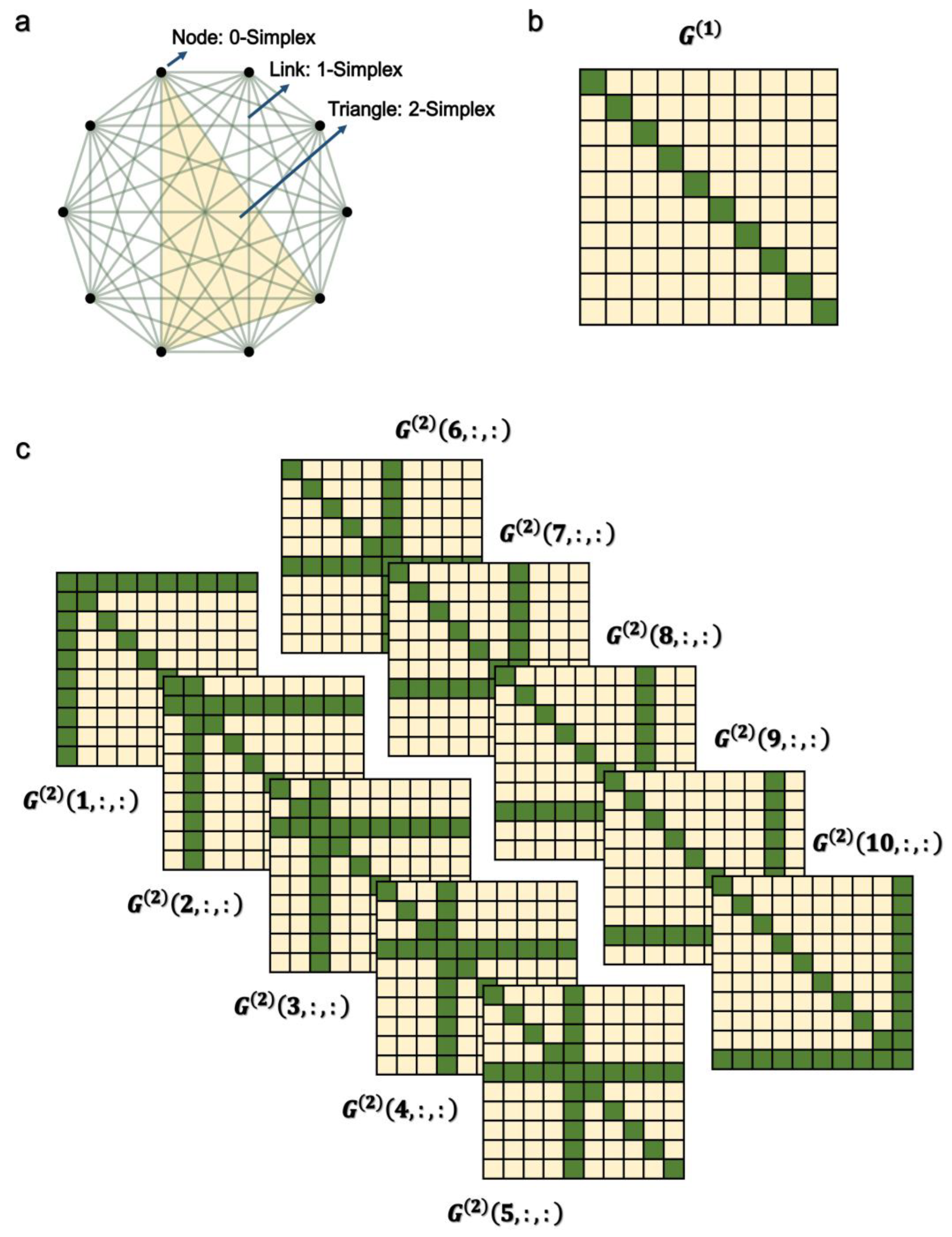
Abstract
:1. Introduction
2. Higher-Order Network Model
3. Results
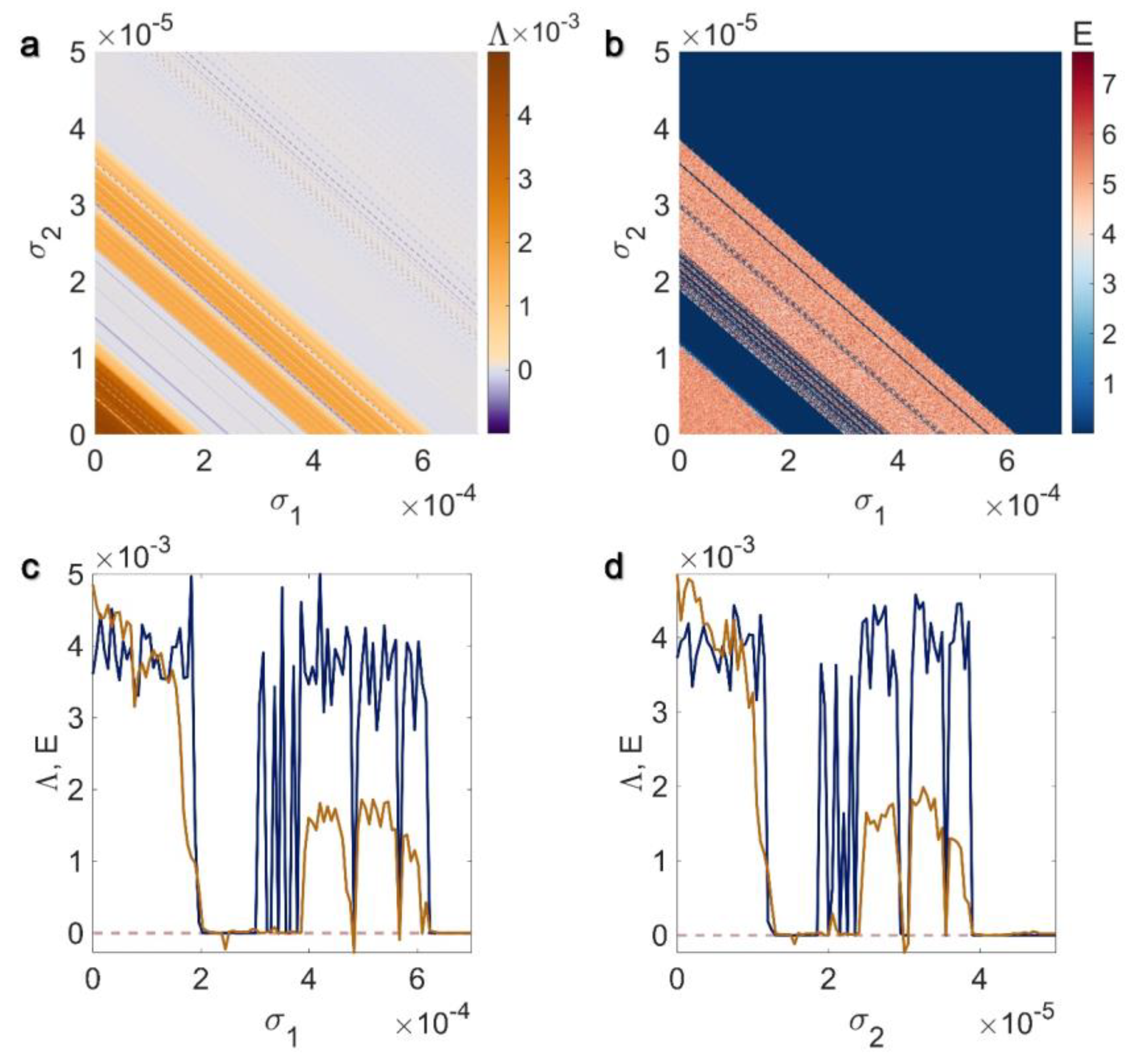
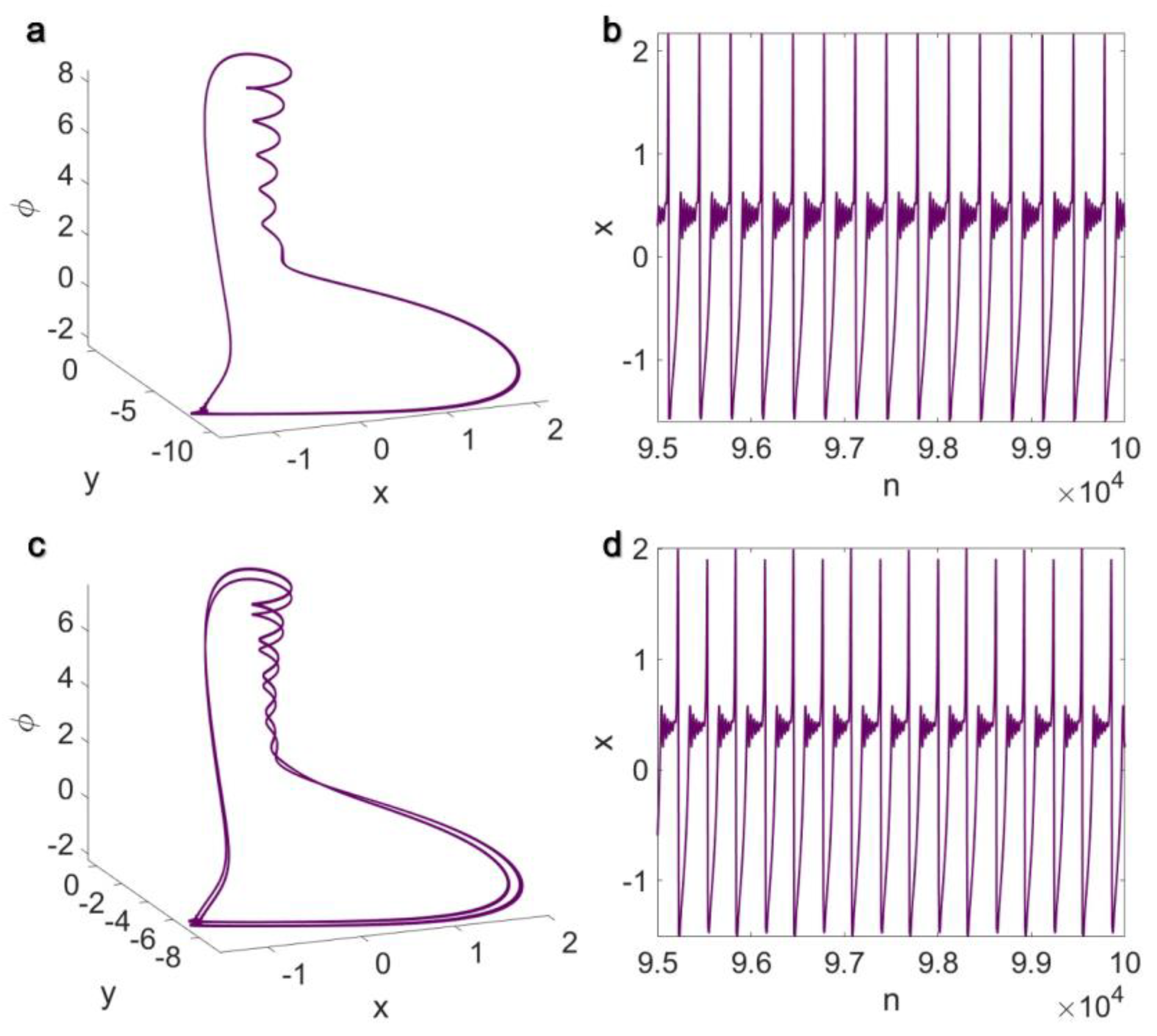
3.1. Electrical Pairwise and Electrical Non-Pairwise Interactions
3.2. Inner Linking Pairwise and Inner Linking Non-Pairwise Interactions
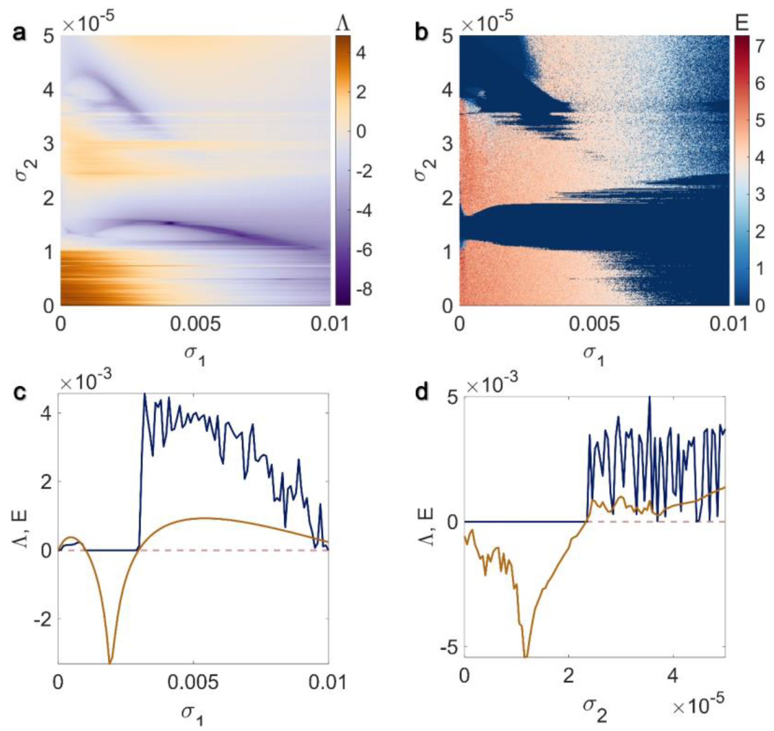
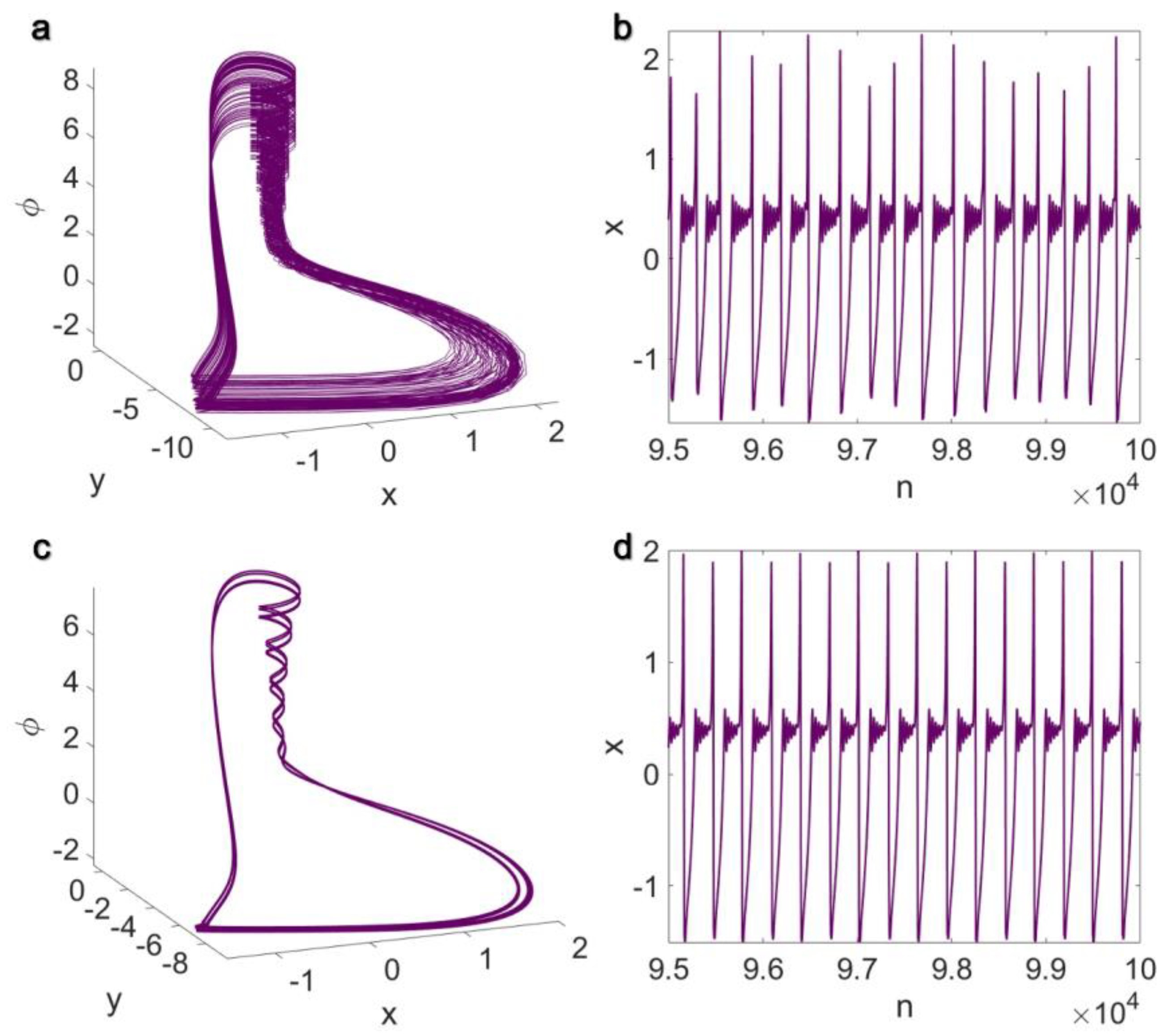
3.3. Chemical Pairwise and Chemical Non-Pairwise Interactions
3.4. Electrical Pairwise and Chemical Non-Pairwise Interactions
3.5. Inner Linking Pairwise and Chemical Non-Pairwise Interactions
4. Conclusions
Author Contributions
Funding
Data Availability Statement
Conflicts of Interest
References
- Uzuntarla, M.; Barreto, E.; Torres, J.J. Inverse stochastic resonance in networks of spiking neurons. PLoS Comput. Biol. 2017, 13, e1005646. [Google Scholar] [CrossRef] [PubMed] [Green Version]
- Uzuntarla, M.; Yilmaz, E.; Ozer, M. Vibrational resonance in a heterogeneous scale free network of neurons. Commun. Nonlinear Sci. Numer. Simul. 2015, 22, 367–374. [Google Scholar] [CrossRef]
- Hong, H.; Choi, M.-Y.; Kim, B.J. Synchronization on small-world networks. Phys. Rev. E 2002, 65, 026139. [Google Scholar] [CrossRef] [PubMed] [Green Version]
- Pecora, L.M.; Carroll, T.L. Synchronization in chaotic systems. Phys. Rev. Lett. 1990, 64, 821. [Google Scholar] [CrossRef]
- Fell, J.; Axmacher, N. The role of phase synchronization in memory processes. Nat. Rev. Neurosci. 2011, 12, 105–118. [Google Scholar] [CrossRef] [PubMed]
- Abreu, R.; Leal, A.; da Silva, F.L.; Figueiredo, P. EEG synchronization measures predict epilepsy-related BOLD-fMRI fluctuations better than commonly used univariate metrics. Clin. Neurophysiol. 2018, 129, 618–635. [Google Scholar] [CrossRef]
- Huang, L.; Chen, Q.; Pecora, L.M. Generic behavior of master-stability functions in coupled nonlinear dynamical systems. Phys. Rev. E 2009, 80, 036204. [Google Scholar] [CrossRef] [Green Version]
- Acharyya, S.; Amritkar, R. Synchronization of nearly identical dynamical systems: Size instability. Phys. Rev. E 2015, 92, 052902. [Google Scholar] [CrossRef] [Green Version]
- Koronovskii, A.; Moskalenko, O.; Hramov, A. Generalized synchronization in the action of a chaotic signal on a periodic system. Tech. Phys. 2014, 59, 629–636. [Google Scholar] [CrossRef]
- Rosenblum, M.G.; Pikovsky, A.S.; Kurths, J. Phase synchronization of chaotic oscillators. Phys. Rev. Lett. 1996, 76, 1804. [Google Scholar] [CrossRef] [Green Version]
- Yi, I.G.; Lee, H.K.; Kim, B.J. Antiphase synchronization of two nonidentical pendulums. Int. J. Bifurc. Chaos 2010, 20, 2179–2184. [Google Scholar] [CrossRef] [Green Version]
- Shahverdiev, E.; Sivaprakasam, S.; Shore, K. Lag synchronization in time-delayed systems. Phys. Lett. A 2002, 292, 320–324. [Google Scholar] [CrossRef]
- Sorrentino, F.; Pecora, L.M.; Roy, R. Complete characterization of the stability of cluster synchronization in complex dynamical networks. Sci. Adv. 2016, 2, e1501737. [Google Scholar] [CrossRef] [PubMed] [Green Version]
- Parastesh, F.; Jafari, S.; Azarnoush, H.; Shahriari, Z.; Wang, Z.; Boccaletti, S.; Perc, M. Chimeras. Phys. Rep. 2021, 898, 1–114. [Google Scholar] [CrossRef]
- Andreev, A.; Frolov, N.; Hramov, A. Chimera state in complex networks of bistable Hodgkin-Huxley neurons. Phys. Rev. E 2019, 100, 022224. [Google Scholar] [CrossRef]
- Ding, K.; Zhu, Q.; Huang, T. Prefixed-Time Local Intermittent Sampling Synchronization of Stochastic Multicoupling Delay Reaction-Diffusion Dynamic Networks. IEEE Trans. Neural Netw. Learn. Syst. 2022, 1–15. [Google Scholar] [CrossRef]
- Kong, F.; Zhu, Q. Fixed-Time Stabilization of Discontinuous Neutral Neural Networks with Proportional Delays via New Fixed-Time Stability Lemmas. IEEE Trans. Neural Netw. Learn. Syst. 2023, 34, 775–785. [Google Scholar] [CrossRef]
- Rao, R.; Lin, Z.; Wu, J. Synchronization of Epidemic Systems with Neumann Boundary Value under Delayed Impulse. Mathematics 2022, 10, 2064. [Google Scholar] [CrossRef]
- Pecora, L.M.; Carroll, T.L. Master Stability Functions for Synchronized Coupled Systems. Phys. Rev. Lett. 1998, 80, 2109–2112. [Google Scholar] [CrossRef] [Green Version]
- Malik, S.; Mir, A.H. Synchronization of hindmarsh rose neurons. Neural Netw. 2020, 123, 372–380. [Google Scholar] [CrossRef]
- Usha, K.; Subha, P. Hindmarsh-Rose neuron model with memristors. Biosystems 2019, 178, 1–9. [Google Scholar] [CrossRef]
- Hussain, I.; Jafari, S.; Perc, M. Synchronization and chimeras in a network of photosensitive FitzHugh–Nagumo neurons. Nonlinear Dyn. 2021, 104, 2711–2721. [Google Scholar] [CrossRef]
- Plotnikov, S.A.; Fradkov, A.L. On synchronization in heterogeneous FitzHugh–Nagumo networks. Chaos Solitons Fractals 2019, 121, 85–91. [Google Scholar] [CrossRef]
- Xu, Y.; Jia, Y.; Ma, J.; Alsaedi, A.; Ahmad, B. Synchronization between neurons coupled by memristor. Chaos Solitons Fractals 2017, 104, 435–442. [Google Scholar] [CrossRef]
- Li, R.; Wang, Z.; Dong, E. A new locally active memristive synapse-coupled neuron model. Nonlinear Dyn. 2021, 104, 4459–4475. [Google Scholar] [CrossRef]
- Fan, W.; Chen, X.; Wu, H.; Li, Z.; Xu, Q. Firing patterns and synchronization of Morris-Lecar neuron model with memristive autapse. AEU-Int. J. Electron. Commun. 2023, 158, 154454. [Google Scholar] [CrossRef]
- Ibarz, B.; Casado, J.M.; Sanjuán, M.A. Sanjuán, Map-based models in neuronal dynamics. Phys. Rep. 2011, 501, 1–74. [Google Scholar] [CrossRef]
- Sun, H.; Cao, H. Complete synchronization of coupled Rulkov neuron networks. Nonlinear Dyn. 2016, 84, 2423–2434. [Google Scholar] [CrossRef]
- Wang, C.; Cao, H. Stability and chaos of Rulkov map-based neuron network with electrical synapse. Commun. Nonlinear Sci. Numer. Simul. 2015, 20, 536–545. [Google Scholar] [CrossRef]
- Hu, D.; Cao, H. Stability and synchronization of coupled Rulkov map-based neurons with chemical synapses. Commun. Nonlinear Sci. Numer. Simul. 2016, 35, 105–122. [Google Scholar] [CrossRef]
- Ge, P.; Cao, H. Synchronization of Rulkov neuron networks coupled by excitatory and inhibitory chemical synapses. Chaos 2019, 29, 023129. [Google Scholar] [CrossRef]
- Rakshit, S.; Ray, A.; Bera, B.K.; Ghosh, D. Synchronization and firing patterns of coupled Rulkov neuronal map. Nonlinear Dyn. 2018, 94, 785–805. [Google Scholar] [CrossRef]
- Mehrabbeik, M.; Parastesh, F.; Ramadoss, J.; Rajagopal, K.; Namazi, H.; Jafari, S. Synchronization and chimera states in the network of electrochemically coupled memristive Rulkov neuron maps. Math. Biosci. Eng. 2021, 18, 9394–9409. [Google Scholar] [CrossRef] [PubMed]
- Li, K.; Bao, B.; Ma, J.; Bao, H. Synchronization transitions in a discrete memristor-coupled bi-neuron model. Chaos Solitons Fractals 2022, 165, 112861. [Google Scholar] [CrossRef]
- Wang, S.; Wei, Z. Synchronization of coupled memristive Hindmarsh–Rose maps under different coupling conditions. AEU-Int. J. Electron. Commun. 2023, 161, 154561. [Google Scholar] [CrossRef]
- Fan, W.; Wu, H.; Li, Z.; Xu, Q. Synchronization and chimera in a multiplex network of Hindmarsh–Rose neuron map with flux-controlled memristor. Eur. Phys. J. Spec. Top. 2022, 231, 4131–4141. [Google Scholar] [CrossRef]
- Ince, R.A.A.; Montani, F.; Arabzadeh, E.; Diamond, M.E.; Panzeri, S. On the presence of high-order interactions among somatosensory neurons and their effect on information transmission. J. Phys. Conf. Ser. 2009, 197, 012013. [Google Scholar] [CrossRef]
- Böhle, T.; Kuehn, C.; Jost, J. Coupled hypergraph maps and chaotic cluster synchronization. Europhys. Lett. 2021, 136, 40005. [Google Scholar] [CrossRef]
- Mulas, R.; Kuehn, C.; Jost, J. Coupled dynamics on hypergraphs: Master stability of steady states and synchronization. Phys. Rev. E 2020, 101, 062313. [Google Scholar] [CrossRef]
- Carletti, T.; Fanelli, D.; Nicoletti, S. Dynamical systems on hypergraphs. J. Phys. Complexity 2020, 1, 035006. [Google Scholar] [CrossRef]
- Gambuzza, L.V.; Di Patti, F.; Gallo, L.; Lepri, S.; Romance, M.; Criado, R.; Frasca, M.; Latora, V.; Boccaletti, S. Stability of synchronization in simplicial complexes. Nat. Commun. 2021, 12, 1255. [Google Scholar] [CrossRef]
- Parastesh, F.; Mehrabbeik, M.; Rajagopal, K.; Jafari, S.; Perc, M. Synchronization in Hindmarsh–Rose neurons subject to higher-order interactions. Chaos 2022, 32, 013125. [Google Scholar] [CrossRef]
- Anwar, M.S.; Ghosh, D. Stability of synchronization in simplicial complexes with multiple interaction layers. Phys. Rev. E 2022, 106, 034314. [Google Scholar] [CrossRef]
- Mirzaei, S.; Mehrabbeik, M.; Rajagopal, K.; Jafari, S.; Chen, G. Synchronization of a higher-order network of Rulkov maps. Chaos 2022, 32, 123133. [Google Scholar] [CrossRef] [PubMed]
- Tlaie, A.; Leyva, I.; Sendiña-Nadal, I. High-order couplings in geometric complex networks of neurons. Phys. Rev. E 2019, 100, 052305. [Google Scholar] [CrossRef] [Green Version]
- Skardal, P.S.; Arenas, A. Higher order interactions in complex networks of phase oscillators promote abrupt synchronization switching. Commun. Phys. 2020, 3, 218. [Google Scholar] [CrossRef]
- Bao, H.; Hua, Z.; Liu, W.; Bao, B. Discrete memristive neuron model and its interspike interval-encoded application in image encryption. Sci. China Technol. Sci. 2021, 64, 2281–2291. [Google Scholar] [CrossRef]
- Bao, H.; Hu, A.; Liu, W.; Bao, B. Hidden bursting firings and bifurcation mechanisms in memristive neuron model with threshold electromagnetic induction. IEEE Trans. Neural Netw. Learn. Syst. 2019, 31, 502–511. [Google Scholar] [CrossRef] [PubMed]


Disclaimer/Publisher’s Note: The statements, opinions and data contained in all publications are solely those of the individual author(s) and contributor(s) and not of MDPI and/or the editor(s). MDPI and/or the editor(s) disclaim responsibility for any injury to people or property resulting from any ideas, methods, instructions or products referred to in the content. |
© 2023 by the authors. Licensee MDPI, Basel, Switzerland. This article is an open access article distributed under the terms and conditions of the Creative Commons Attribution (CC BY) license (https://creativecommons.org/licenses/by/4.0/).
Share and Cite
Mehrabbeik, M.; Ahmadi, A.; Bakouie, F.; Jafari, A.H.; Jafari, S.; Ghosh, D. The Impact of Higher-Order Interactions on the Synchronization of Hindmarsh–Rose Neuron Maps under Different Coupling Functions. Mathematics 2023, 11, 2811. https://doi.org/10.3390/math11132811
Mehrabbeik M, Ahmadi A, Bakouie F, Jafari AH, Jafari S, Ghosh D. The Impact of Higher-Order Interactions on the Synchronization of Hindmarsh–Rose Neuron Maps under Different Coupling Functions. Mathematics. 2023; 11(13):2811. https://doi.org/10.3390/math11132811
Chicago/Turabian StyleMehrabbeik, Mahtab, Atefeh Ahmadi, Fatemeh Bakouie, Amir Homayoun Jafari, Sajad Jafari, and Dibakar Ghosh. 2023. "The Impact of Higher-Order Interactions on the Synchronization of Hindmarsh–Rose Neuron Maps under Different Coupling Functions" Mathematics 11, no. 13: 2811. https://doi.org/10.3390/math11132811