Towards Higher-Order Zeroing Neural Networks for Calculating Quaternion Matrix Inverse with Application to Robotic Motion Tracking

Abstract

The efficient solution of the time-varying quaternion matrix inverse (TVQ-INV) is a challenging but crucial topic due to the significance of quaternions in many disciplines, including physics, engineering, and computer science. The main goal of this research is to employ the higher-order zeroing neural network (HZNN) strategy to address the TVQ-INV problem. HZNN is a family of zeroing neural network models that correlates to the hyperpower family of iterative methods with adjustable convergence order. Particularly, three novel HZNN models are created in order to solve the TVQ-INV both directly in the quaternion domain and indirectly in the complex and real domains. The noise-handling version of these models is also presented, and the performance of these models under various types of noises is theoretically and numerically tested. The effectiveness and practicality of these models are further supported by their use in robotic motion tracking. According to the principal results, each of these six models can solve the TVQ-INV effectively, and the HZNN strategy offers a faster convergence rate than the conventional zeroing neural network strategy.

1. Introduction

The real-time solution to the matrix inverse [1,2], which frequently arises in robotics [3], game theory [4], nonlinear systems [5], optimal control [6,7], and neural networks [8], has attracted a lot of interest in recent times. Quaternions, on the other hand, are crucial in a wide range of domains, such as computer graphics [9], signal processing [10], human motion modeling [11], robotics [12,13], navigation [14], quantum mechanics [15], electromagnetism [16], and mathematical physics [17,18]. Let ${\mathbb{H}}^{n\times n}$ present the set of all $n\times n$ matrices on the quaternion skew field $\mathbb{H}=\{{\gamma }_1+{\mathit{\gamma }}_{2}l+{\gamma }_{3}j+{\gamma }_{4}k|l^2=j^2=k^2=ljk=-1,{\gamma }_1,{\gamma }_2,{\gamma }_3,{\gamma }_4\in \mathbb{R}\}$. Considering that $\tilde{A}\in {\mathbb{H}}^{n\times n}$, its inverse matrix is denoted by ${\tilde{A}}^{-1}$ and it is the only solution $\tilde{X}$ that satisfies the next equation [19,20]:

$$\tilde{A}\tilde{X}=I_n,$$

(1)

where $I_n$ is the identity $n\times n$ matrix.

Recently, research has begun to focus on time-varying quaternion (TVQ) problems involving matrices, such as the inversion of TVQ matrices [21], solving the dynamic TVQ Sylvester matrix equation [22], addressing the TVQ constrained matrix least-squares problem [23], and solving the TVQ linear matrix equation for square matrices [24]. Furthermore, real-world applications involving TVQ matrices are employed in the kinematically redundant manipulator of robotic joints [25,26], such as the control of wearable robotic knee system [27] and control of robotic arm [13], chaotic systems synchronization [23], mobile manipulator control [21], and image restoration [24]. All of these studies have one thing in common: they all use the zeroing neural network (ZNN) approach to derive the solution.

ZNNs are a subset of recurrent neural networks that are especially good at parallel processing and are used to address time-varying issues. They were initially developed by Zhang et al. to handle the problem of time-varying matrix inversion [28], but their subsequent iterations were dynamic models used to compute the time-varying MP-inverse of full-row/column rank matrices [29,30,31,32] in the real and complex domain. Today their use has expanded to include the resolution of generalized inversion issues, including time-varying Drazin inverse [33], time-varying ML-weighted pseudoinverse [34], time-varying outer inverse [35], time-varying pseudoinverse [36], and core and core-EP inverse [37]. Their use has expanded to include the resolution of linear programming tasks [38], quadratic programming tasks [39,40], systems of nonlinear equations [41,42], and systems of linear equations [43,44]. The creation of a ZNN model typically involves two fundamental steps. First, one defines an error matrix equation (EME) function $E\left(t\right)$. Second, the next ZNN dynamical system (under the linear activation) function must be used:

$$\dot{E}\left(t\right)=-\lambda E\left(t\right),$$

(2)

where the operator $\left(\dot{}\right)$ denotes the time derivative. Additionally, the design parameter $\lambda >0$ is a real number that regulates the model’s convergence speed. For instance, a greater value for $\lambda$ will increase the model’s convergence speed [45,46,47]. It is important to point out that continual learning is defined as learning continually from non-stationary data while simultaneously transferring and preserving prior knowledge. It is true that as time evolves, the architecture of ZNN relies on driving each element of the error function $E\left(t\right)$ to zero. The continuous-time learning rule, which is the consequence of the definition of the EME function (2), is used to do this. Therefore, it is possible to think of the error function as a tool for tracking the learning of ZNN models.

1.1. The Higher-Order ZNN Design

In recent years, there has been a great deal of research and development into the hyperpower iteration family [48,49,50,51,52]. However, various continuous-time higher-order ZNN (HZNN) models were presented and studied in Refs. [36,43,53] due to the fact that iterative approaches are realizable to discrete-time models and that these methods often require starting points that are approximated and sometimes may not be easily supplied. Beginning with the subsequent hyperpower iterations with order $p\ge 2$ [36,52]:

$$W_{k+1}=W_k\sum _{i=0}^{p-1}{E}_k^i,$$

(3)

where $E_k\in {\mathbb{R}}^{n\times n}$ denotes a suitable time-invariant EME, it is possible to extend the time-invariant (3) to a time-varying scenario. That is, taking into account the next EME:

$$E_H^p\left(t\right)=\sum _{i=1}^{p-1}{E}^i\left(t\right),$$

(4)

where $E^i\left(t\right)\in {\mathbb{R}}^{n\times n}$ and $p\ge 2$, the ZNN architecture and the hyperpower iterations approach can be combined to find the online solution to a time-varying problem. This yields the next comprehensive HZNN dynamical evolution [36,43,53] (under the linear activation function):

$$\dot{E}\left(t\right)\approx -\lambda E_H^p\left(t\right).$$

(5)

1.2. The Noise-Handling Higher-Order ZNN Design

Every form of noise has a significant impact on the precision of the suggested ZNN methods, and any preliminary processing for a noise reduction attaches time, sacrificing desired real-time demands. As a result, an enhanced noise-handling model for handling time-varying problems was developed in Ref. [54]. The noise-handling ZNN (NZNN) dynamical system below was introduced in particular [54]:

$$\dot{E}\left(t\right)=-\lambda E\left(t\right)-\zeta {\int }_0^{t}E\left(\tau \right)\mathrm{d}\tau +N\left(t\right),$$

(6)

where $\zeta$ and $\lambda$ are design parameters that track NZNN convergence, while $N\left(t\right)$ stands for the proper dimensional matrix-form noises. It should be noted that [43] introduced and examined the generalization of the NZNN architecture to the NHZNN formulation for estimating a time-varying problem. The generic NHZNN dynamical evolution may be acquired by integrating the hyperpower iterations process and the NZNN design, using the same rationale as the HZNN design in (4) and (5):

$$\dot{E}\left(t\right)\approx -\lambda E_H^p\left(t\right)-\zeta {\int }_0^t{E}_H^p\left(\tau \right)\mathrm{d}\tau +N\left(t\right).$$

(7)

1.3. Problem Formulation and Key Contributions

In this paper, the TVQ inverse (TVQ-INV) problem will be addressed using the HZNN and NHZNN approaches. Particularly, the following TVQ matrix equations problem is taken into consideration for computing the TVQ-INV of any nonsingular $\tilde{A}\left(t\right)\in {\mathbb{H}}^{n\times n}$ [19,20]:

$$I_n-\tilde{A}\left(t\right)\tilde{X}\left(t\right)={\mathbf{0}}_n,$$

(8)

where the TVQ matrix $\tilde{X}\left(t\right)=X_1\left(t\right)+X_2\left(t\right)l+X_3\left(t\right)j+X_4\left(t\right)k\in {\mathbb{H}}^{n\times n}$, with $X_i\left(t\right)\in {\mathbb{R}}^{n\times n}$ for $i=1,2,3,4$, is the TVQ matrix of interest, ${\mathbf{0}}_n$ refers to the zero $n\times n$ matrix and $t\in [0,t_f)\subseteq [0,+\infty )$ is the time. Additionally, we consider that $\tilde{A}\left(t\right)$ is a smoothly time-varying matrix and its time derivative is either given or can be accurately estimated. It is important to note that (8) is the TVQ-INV problem and it is satisfied only for $\tilde{X}\left(t\right)={\tilde{A}}^{-1}\left(t\right)$. Of greater significance, we will determine whether a direct solution in the quaternion domain or an indirect solution through representation in the complex and real domains is more efficient. To do this, we will create three HZNN and three NHZNN models, one for each domain, and rigorously validate them on two numerical simulations under various types of noises and a real-world application involving robotic motion tracking. By doing theoretical analysis of all presented models, this research strengthens the existing body of literature.

The following notations are employed in the remainder of this article: ${\mathbf{0}}_{u\times n}$ refers to the zero $u\times n$ matrix; ${\mathbf{1}}_n$ refers to the $n\times 1$ matrix of ones; ${∥·∥}_F$ is the matrix Frobenius norm; $\mathrm{vec}(·)$ denotes the vectorization process; ⊙ denotes the elementwise multiplication; ⊗ denotes the Kronecker product; the operator ${\left(\right)}^{\mathrm{T}}$ implies transposition.

The key contributions of the paper are listed next:

(1)

For the first time, the TVQ-INV problem is addressed through the HZNN and NHZNN approaches;

(2)

With the purpose of addressing the TVQ-INV problem, three novel HZNN models and three novel NHZNN models are provided;

(3)

The models are subjected to a theoretical analysis that validates them;

(4)

Numerical simulations and applications under various types of noises are carried out to complement the theoretical concepts.

The rest of the article is divided into the following sections. Section 2 presents the three HZNN and three NHZNN models, while their theoretical analysis is presented in Section 3. Numerical simulations and applications are explored in Section 4 and, finally, Section 5 provides the concluding thoughts and comments.

2. Higher Order and Noise-Handling ZNN Models in Solving the TVQ-INV

Three HZNN models will be created in this section, each of which will operate in a distinct domain. We consider that $\tilde{A}\left(t\right)\in {\mathbb{H}}^{n\times n}$ is a differentiable TVQ matrix and $\tilde{X}\left(t\right)\in {\mathbb{H}}^{n\times n}$ is the unknown TVQ matrix to be found.

2.1. The HZNNQ${}_p$ Model

The product of two TVQ matrices, $\tilde{A}\left(t\right)=A_1\left(t\right)+A_2\left(t\right)l+A_3\left(t\right)j+A_4\left(t\right)k\in {\mathbb{H}}^{n\times n}$ and $\tilde{X}\left(t\right)=X_1\left(t\right)+X_2\left(t\right)l+X_3\left(t\right)j+X_4\left(t\right)k\in {\mathbb{H}}^{n\times n}$, with $A_i\left(t\right),X_i\left(t\right)\in {\mathbb{R}}^{n\times n}$ for $i=1,\dots ,4$, is:

$$\tilde{A}\left(t\right)\tilde{X}\left(t\right)=\tilde{Z}\left(t\right)=Z_1\left(t\right)+Z_2\left(t\right)l+Z_3\left(t\right)j+Z_4\left(t\right)k\in {\mathbb{H}}^{n\times n}$$

(9)

where

$$\begin{gathered} Z_1\left(t\right)=A_1\left(t\right)X_1\left(t\right)-A_2\left(t\right)X_2\left(t\right)-A_3\left(t\right)X_3\left(t\right)-A_4\left(t\right)X_4\left(t\right), \\ {Z}_2\left(t\right)=A_1\left(t\right)X_2\left(t\right)+A_2\left(t\right)X_1\left(t\right)+A_3\left(t\right)X_4\left(t\right)-A_4\left(t\right)X_3\left(t\right), \\ {Z}_3\left(t\right)=A_1\left(t\right)X_3\left(t\right)+A_3\left(t\right)X_1\left(t\right)+A_4\left(t\right)X_2\left(t\right)-A_2\left(t\right)X_4\left(t\right), \\ {Z}_4\left(t\right)=A_1\left(t\right)X_4\left(t\right)+A_4\left(t\right)X_1\left(t\right)+A_2\left(t\right)X_3\left(t\right)-A_3\left(t\right)X_2\left(t\right), \end{gathered}$$

(10)

with $Z_i\left(t\right)\in {\mathbb{R}}^{n\times n}$ for $i=1,\dots ,4$. According to (8), setting $\tilde{Z}\left(t\right)=I$ in the case of TVQ-INV, the next system of equations is satisfied:

$$\left\{\begin{array}{c}{A}_1\left(t\right)X_1\left(t\right)-A_2\left(t\right)X_2\left(t\right)-A_3\left(t\right)X_3\left(t\right)-A_4\left(t\right)X_4\left(t\right)=I_n,\hfill \\ A_2\left(t\right)X_1\left(t\right)+A_1\left(t\right)X_2\left(t\right)-A_4\left(t\right)X_3\left(t\right)+A_3\left(t\right)X_4\left(t\right)={\mathbf{0}}_n,\hfill \\ A_3\left(t\right)X_1\left(t\right)+A_4\left(t\right)X_2\left(t\right)+A_1\left(t\right)X_3\left(t\right)-A_2\left(t\right)X_4\left(t\right)={\mathbf{0}}_n,\hfill \\ A_4\left(t\right)X_1\left(t\right)-A_3\left(t\right)X_2\left(t\right)+A_2\left(t\right)X_3\left(t\right)+A_1\left(t\right)X_4\left(t\right)={\mathbf{0}}_n,\hfill \end{array}\right.$$

(11)

where $X_i\left(t\right)$, $i=1,\dots ,4$, are the unknown matrices of interest. Then, setting

$$\begin{gathered} B\left(t\right)=\left[\begin{array}{cccc}{A}_1\left(t\right)& -A_2\left(t\right)& -A_3\left(t\right)& -A_4\left(t\right)\\ A_2\left(t\right)& A_1\left(t\right)& -A_4\left(t\right)& A_3\left(t\right)\\ A_3\left(t\right)& A_4\left(t\right)& A_1\left(t\right)& -A_2\left(t\right)\\ A_4\left(t\right)& -A_3\left(t\right)& A_2\left(t\right)& A_1\left(t\right)\end{array}\right]\in {\mathbb{R}}^{4n\times 4n}, \\ Y\left(t\right)=\left[\begin{array}{c}{X}_1\left(t\right)\\ X_2\left(t\right)\\ X_3\left(t\right)\\ X_4\left(t\right)\end{array}\right]\in {\mathbb{R}}^{4n\times n},\widehat{I}=\left[\begin{array}{c}{I}_n\\ {\mathbf{0}}_n\\ {\mathbf{0}}_n\\ {\mathbf{0}}_n\end{array}\right]\in {\mathbb{R}}^{4n\times n}, \end{gathered}$$

(12)

we have the following EME:

$$E\left(t\right)=\widehat{I}-B\left(t\right)Y\left(t\right).$$

(13)

The fact that $E\left(t\right)\in {\mathbb{R}}^{4n\times n}$ is not a square EME and cannot be applied to the HZNN design in (5) is significant. Because of this, we may replace the $E\left(t\right)$ of (13) into the following equation without losing generality:

$$E\left(t\right)=(\widehat{I}-B\left(t\right)Y\left(t\right)){\widehat{I}}^{\mathrm{T}},$$

(14)

and its first time derivative is:

$$\dot{E}\left(t\right)=-(\dot{B}\left(t\right)Y\left(t\right)+B\left(t\right)\dot{Y}\left(t\right)){\widehat{I}}^{\mathrm{T}}.$$

(15)

Then, the following EME can be defined based on the HZNN design:

$$E_H^p\left(t\right)=\sum _{i=1}^{p-1}{\left((\widehat{I}-B\left(t\right)Y\left(t\right)){\widehat{I}}^{\mathrm{T}}\right)}^i,$$

(16)

while its derivative is:

$${\dot{E}}_H^p\left(t\right)=\sum _{i=1}^{p-1}\sum _{j=0}^{i-1}{\left((\widehat{I}-B\left(t\right)Y\left(t\right)){\widehat{I}}^{\mathrm{T}}\right)}^j\left(-(\dot{B}\left(t\right)Y\left(t\right)+B\left(t\right)\dot{Y}\left(t\right)){\widehat{I}}^{\mathrm{T}}\right){\left((\widehat{I}-B\left(t\right)Y\left(t\right)){\widehat{I}}^{\mathrm{T}}\right)}^{i-1-j},$$

(17)

the replacement $(\widehat{I}-B\left(t\right)Y\left(t\right)){\widehat{I}}^{\mathrm{T}}={\mathbf{0}}_{4n\times 4n}$ in (17) converts each of the summations into the null matrix, beside the summand referring to $j=0$, $i=1$. So, (17) is estimated as:

$${\dot{E}}_H^p\left(t\right)\approx -(\dot{B}\left(t\right)Y\left(t\right)+B\left(t\right)\dot{Y}\left(t\right)){\widehat{I}}^{\mathrm{T}}=\dot{E}\left(t\right).$$

(18)

The next outcome is obtained by substituting $E_H^p\left(t\right)$ of (16) and ${\dot{E}}_H^p\left(t\right)$ of (17) into (5):

$$-(\dot{B}\left(t\right)Y\left(t\right)+B\left(t\right)\dot{Y}\left(t\right)){\widehat{I}}^{\mathrm{T}}=-\lambda \sum _{i=1}^{p-1}{E}^i\left(t\right),$$

(19)

and solving in terms of $\dot{Y}\left(t\right)$ yields:

$$-B\left(t\right)\dot{Y}\left(t\right){\widehat{I}}^{\mathrm{T}}=-\lambda \sum _{i=1}^{p-1}{E}^i\left(t\right)+\dot{B}\left(t\right)Y\left(t\right){\widehat{I}}^{\mathrm{T}}.$$

(20)

The dynamic model of (20) can then be made simpler with the use of vectorization and Kronecker product:

$$-(\widehat{I}\otimes B\left(t\right))\mathrm{vec}(\dot{Y}\left(t\right))=\mathrm{vec}(-\lambda \sum _{i=1}^{p-1}{E}^i\left(t\right)+\dot{B}\left(t\right)Y\left(t\right){\widehat{I}}^{\mathrm{T}}).$$

(21)

Furthermore, after setting:

$$\begin{array}{l}{K}_1\left(t\right)=-(\widehat{I}\otimes B\left(t\right))\in {\mathbb{R}}^{16n^2\times 4n^2},M_1\left(t\right)=K_1^{\mathrm{T}}\left(t\right)K_1\left(t\right)\in {\mathbb{R}}^{4n^2\times 4n^2},\\ K_2\left(t\right)=\mathrm{vec}(-\lambda {\displaystyle \sum _{i=1}^{p-1}}{E}^i\left(t\right)+\dot{B}\left(t\right)Y\left(t\right){\widehat{I}}^{\mathrm{T}})\in {\mathbb{R}}^{16n^2},M_2\left(t\right)=K_1^{\mathrm{T}}\left(t\right)K_2\left(t\right)\in {\mathbb{R}}^{4n^2},\\ \mathbf{y}\left(t\right)=\mathrm{vec}\left(Y\left(t\right)\right)\in {\mathbb{R}}^{4n^2},\dot{\mathbf{y}}\left(t\right)=\mathrm{vec}\left(\dot{Y}\left(t\right)\right)\in {\mathbb{R}}^{4n^2},\end{array}$$

(22)

we arrive to the subsequent HZNN model:

$$M_1\left(t\right)\dot{\mathbf{y}}\left(t\right)=M_2\left(t\right).$$

(23)

The suggested HZNN model to be utilized when addressing the TVQ-INV of (8) is the dynamic model of (23), denoted by the notation HZNNQ${}_p$.

2.2. The NHZNNQ${}_p$ Model

Additionally, the next outcome is obtained by substituting $E_H^p\left(t\right)$ of (16) and ${\dot{E}}_H^p\left(t\right)$ of (17) into (7):

$$-(\dot{B}\left(t\right)Y\left(t\right)+B\left(t\right)\dot{Y}\left(t\right)){\widehat{I}}^{\mathrm{T}}=-\lambda \sum _{i=1}^{p-1}{E}^i\left(t\right)-\zeta {\int }_0^t{E}_H^p\left(\tau \right)\mathrm{d}\tau +N\left(t\right),$$

(24)

and solving in terms of $\dot{Y}\left(t\right)$ outputs:

$$-B\left(t\right)\dot{Y}\left(t\right){\widehat{I}}^{\mathrm{T}}=-\lambda \sum _{i=1}^{p-1}{E}^i\left(t\right)+\dot{B}\left(t\right)Y\left(t\right){\widehat{I}}^{\mathrm{T}}-\zeta {\int }_0^t{E}_H^p\left(\tau \right)\mathrm{d}\tau +N\left(t\right).$$

(25)

The dynamic model of (25) can then be made simpler with the use of vectorization and Kronecker product:

$$-(\widehat{I}\otimes B\left(t\right))\mathrm{vec}\left(\dot{Y}\left(t\right)\right)=\mathrm{vec}(-\lambda \sum _{i=1}^{p-1}{E}^i\left(t\right)+\dot{B}\left(t\right)Y\left(t\right){\widehat{I}}^{\mathrm{T}}-\zeta {\int }_0^t{E}_H^p\left(\tau \right)\mathrm{d}\tau +N\left(t\right)).$$

(26)

Furthermore, after setting:

$$\begin{array}{l}{r}_q\left(t\right)=\mathrm{vec}\left({\int }_0^t{E}_H^p\left(\tau \right)\mathrm{d}\tau \widehat{I}\right)\in {\mathbb{R}}^{16n^2},{\dot{r}}_q\left(t\right)=\mathrm{vec}({\displaystyle \sum _{i=1}^{p-1}}{E}^i\left(t\right)\widehat{I})\in {\mathbb{R}}^{16n^2},\\ K_3\left(t\right)=\left[\begin{array}{cc}{I}_{4n^2}& {\mathbf{0}}_{4n^2\times 4n^2}\\ {\mathbf{0}}_{16n^2\times 4n^2}& K_1\left(t\right)\end{array}\right]\in {\mathbb{R}}^{20n^2\times 8n^2},M_3\left(t\right)=K_3^{\mathrm{T}}\left(t\right)K_3\left(t\right)\in {\mathbb{R}}^{8n^2\times 8n^2},\\ K_4\left(t\right)=\mathrm{vec}(-\lambda {\displaystyle \sum _{i=1}^{p-1}}{E}^i\left(t\right)+\dot{B}\left(t\right)Y\left(t\right){\widehat{I}}^{\mathrm{T}}+N\left(t\right))-\zeta r_q\left(t\right){\widehat{I}}^{\mathrm{T}}\in {\mathbb{R}}^{16n^2},\\ K_5\left(t\right)=\left[\begin{array}{c}{r}_q\left(t\right)\\ K_4\left(t\right)\end{array}\right]\in {\mathbb{R}}^{16n^2},M_4\left(t\right)=K_3^{\mathrm{T}}\left(t\right)K_5\left(t\right)\in {\mathbb{R}}^{8n^2},\\ {\mathbf{y}}_N\left(t\right)=\left[\begin{array}{c}{r}_q\left(t\right)\\ \mathbf{y}\left(t\right)\end{array}\right]\in {\mathbb{R}}^{8n^2},{\dot{\mathbf{y}}}_N\left(t\right)=\left[\begin{array}{c}{\dot{r}}_q\left(t\right)\\ \dot{\mathbf{y}}\left(t\right)\end{array}\right]\in {\mathbb{R}}^{8n^2},\end{array}$$

(27)

we arrive to the subsequent NHZNN model:

$$M_3\left(t\right){\dot{\mathbf{y}}}_N\left(t\right)=M_4\left(t\right).$$

(28)

The suggested NHZNN model to be utilized when addressing the TVQ-INV of (8) under various types of noises is the dynamic model of (28), denoted by the notation NHZNNQ${}_p$.

2.3. The HZNNQC${}_p$ Model

The following is a complex representation of the TVQ matrix $\tilde{A}\left(t\right)$ [22,55]:

$$\check{A}\left(t\right)=\left[\begin{array}{cc}{A}_1\left(t\right)-A_4\left(t\right)l& -A_3\left(t\right)-A_2\left(t\right)l\\ A_3\left(t\right)-A_2\left(t\right)l& A_1\left(t\right)+A_4\left(t\right)l\end{array}\right]\in {\mathbb{C}}^{2n\times 2n}.$$

(29)

Taking into account that the complex representation of the TVQ matrix acquired by multiplying two TVQ matrices is similar to the TVQ matrix acquired by multiplying the complex representations of two TVQ matrices (Theorem 1 in Ref. [22]), addressing (8) is equivalent to addressing the complex matrix equation:

$$\check{A}\left(t\right)\check{X}\left(t\right)=I_{2n},$$

(30)

where $\check{X}\left(t\right)\in {\mathbb{C}}^{2n\times 2n}$, is the unknown matrix of interest, i.e., the complex representation of the TVQ matrix $\tilde{X}\left(t\right)$. Therefore, we set the next EME:

$$E\left(t\right)=I_{2n}-\check{A}\left(t\right)\check{X}\left(t\right),$$

(31)

and its first time derivative is:

$$\dot{E}\left(t\right)=-\dot{\check{A}}\left(t\right)\check{X}\left(t\right)-\check{A}\left(t\right)\dot{\check{X}}\left(t\right).$$

(32)

Then, the following EME can be defined based on the HZNN design:

$$E_H^p\left(t\right)=\sum _{i=1}^{p-1}{\left(I_{2n}-\check{A}\left(t\right)\check{X}\left(t\right)\right)}^i,$$

(33)

while its derivative is:

$${\dot{E}}_H^p\left(t\right)=\sum _{i=1}^{p-1}\sum _{j=0}^{i-1}{\left(I_{2n}-\check{A}\left(t\right)\check{X}\left(t\right)\right)}^j\left(-\check{A}\left(t\right)\dot{\check{X}}\left(t\right)-\dot{\check{A}}\left(t\right)\check{X}\left(t\right)\right){\left(I_{2n}-\check{A}\left(t\right)\check{X}\left(t\right)\right)}^{i-1-j},$$

(34)

the replacement $I_{2n}-\check{A}\left(t\right)\check{X}\left(t\right)={\mathbf{0}}_{2n\times 2n}$ in (34) converts each of the summations into the null matrix, beside the summand referring to $j=0$, $i=1$. So, (34) is estimated as:

$${\dot{E}}_H^p\left(t\right)\approx -\check{A}\left(t\right)\dot{\check{X}}\left(t\right)-\dot{\check{A}}\left(t\right)\check{X}\left(t\right)=\dot{E}\left(t\right).$$

(35)

The next outcome is obtained by substituting $E_H^p\left(t\right)$ of (33) and ${\dot{E}}_H^p\left(t\right)$ of (34) into (5):

$$-\check{A}\left(t\right)\dot{\check{X}}\left(t\right)-\dot{\check{A}}\left(t\right)\check{X}\left(t\right)=-\lambda \sum _{i=1}^{p-1}{E}^i\left(t\right),$$

(36)

and solving in terms of $\dot{\check{X}}\left(t\right)$ outputs:

$$-\check{A}\left(t\right)\dot{\check{X}}\left(t\right)=-\lambda \sum _{i=1}^{p-1}{E}^i\left(t\right)+\dot{\check{A}}\left(t\right)\check{X}\left(t\right).$$

(37)

The dynamic model of (37) can then be made simpler with the use of vectorization and Kronecker product:

$$-(I_{2n}\otimes \check{A})\mathrm{vec}(\dot{\check{X}}\left(t\right))=\mathrm{vec}(-\lambda \sum _{i=1}^{p-1}{E}^i\left(t\right)+\dot{\check{A}}\left(t\right)\check{X}\left(t\right))$$

(38)

Furthermore, after setting:

$$\begin{array}{l}{N}_1\left(t\right)=-(I_{2n}\otimes \check{A})\in {\mathbb{C}}^{4n^2\times 4n^2},N_2\left(t\right)=\mathrm{vec}(-\lambda {\displaystyle \sum _{i=1}^{p-1}}{E}^i\left(t\right)+\dot{\check{A}}\left(t\right)\check{X}\left(t\right))\in {\mathbb{C}}^{4n^2},\\ \mathbf{k}\left(t\right)=\mathrm{vec}\left(\check{X}\left(t\right)\right)\in {\mathbb{C}}^{4n^2},\dot{\mathbf{k}}\left(t\right)=\mathrm{vec}\left(\dot{\check{X}}\left(t\right)\right)\in {\mathbb{C}}^{4n^2},\end{array}$$

(39)

we arrive to the subsequent HZNN model:

$$N_1\left(t\right)\dot{\mathbf{k}}\left(t\right)=N_2\left(t\right).$$

(40)

The suggested HZNN model to be utilized when addressing the TVQ-INV of (8) under complex representation of the input TVQ matrix $\tilde{A}\left(t\right)$ is the dynamic model of (40), denoted by the notation HZNNQC${}_p$.

2.4. The NHZNNQC${}_p$ Model

Additionally, the next outcome is obtained by substituting $E_H^p\left(t\right)$ of (33) and ${\dot{E}}_H^p\left(t\right)$ of (34) into (7):

$$-\check{A}\left(t\right)\dot{\check{X}}\left(t\right)-\dot{\check{A}}\left(t\right)\check{X}\left(t\right)=-\lambda \sum _{i=1}^{p-1}{E}^i\left(t\right)-\zeta {\int }_0^t{E}_H^p\left(\tau \right)\mathrm{d}\tau +N\left(t\right),$$

(41)

and solving in terms of $\dot{\check{X}}\left(t\right)$ outputs:

$$-\check{A}\left(t\right)\dot{\check{X}}\left(t\right)=-\lambda \sum _{i=1}^{p-1}{E}^i\left(t\right)+\dot{\check{A}}\left(t\right)\check{X}\left(t\right)-\zeta {\int }_0^t{E}_H^p\left(\tau \right)\mathrm{d}\tau +N\left(t\right).$$

(42)

The dynamic model of (42) can then be made simpler with the use of vectorization and Kronecker product:

$$-(I_{2n}\otimes \check{A})\mathrm{vec}(\dot{\check{X}}\left(t\right))=\mathrm{vec}(-\lambda \sum _{i=1}^{p-1}{E}^i\left(t\right)+\dot{\check{A}}\left(t\right)\check{X}\left(t\right)-\zeta {\int }_0^t{E}_H^p\left(\tau \right)\mathrm{d}\tau +N\left(t\right)).$$

(43)

Furthermore, after setting:

$$\begin{array}{l}{r}_c\left(t\right)=\mathrm{vec}\left({\int }_0^t{E}_H^p\left(\tau \right)\mathrm{d}\tau \right)\in {\mathbb{C}}^{4n^2},{\dot{r}}_c\left(t\right)=\mathrm{vec}({\displaystyle \sum _{i=1}^{p-1}}{E}^i\left(t\right))\in {\mathbb{C}}^{4n^2},\\ N_3\left(t\right)=\left[\begin{array}{cc}{I}_{4n^2}& {\mathbf{0}}_{4n^2\times 4n^2}\\ {\mathbf{0}}_{4n^2\times 4n^2}& N_1\left(t\right)\end{array}\right]\in {\mathbb{C}}^{8n^2\times 8n^2},\\ N_4\left(t\right)=\mathrm{vec}(-\lambda {\displaystyle \sum _{i=1}^{p-1}}{E}^i\left(t\right)+\dot{\check{A}}\left(t\right)\check{X}\left(t\right)+N\left(t\right))-\zeta r_c\left(t\right)\in {\mathbb{C}}^{8n^2},\\ {\mathbf{k}}_N\left(t\right)=\left[\begin{array}{c}{r}_c\left(t\right)\\ \mathbf{k}\left(t\right)\end{array}\right]\in {\mathbb{C}}^{8n^2},{\dot{\mathbf{k}}}_N\left(t\right)=\left[\begin{array}{c}{\dot{r}}_c\left(t\right)\\ \dot{\mathbf{k}}\left(t\right)\end{array}\right]\in {\mathbb{C}}^{8n^2},\end{array}$$

(44)

we arrive to the subsequent NHZNN model:

$$N_3\left(t\right){\dot{\mathbf{k}}}_N\left(t\right)=N_4\left(t\right).$$

(45)

The suggested NHZNN model to be utilized when addressing the TVQ-INV of (8) under various types of noises is the dynamic model of (45), denoted by the notation NHZNNQC${}_p$.

2.5. The HZNNQR${}_p$ Model

The following is a real representation of the TVQ matrix $\tilde{A}\left(t\right)$ [24]:

$$A\left(t\right)=\left[\begin{array}{cccc}{A}_1\left(t\right)& A_4\left(t\right)& -A_3\left(t\right)& A_2\left(t\right)\\ -A_4\left(t\right)& A_1\left(t\right)& -A_2\left(t\right)& -A_3\left(t\right)\\ A_3\left(t\right)& A_2\left(t\right)& A_1\left(t\right)& -A_4\left(t\right)\\ -A_2\left(t\right)& A_3\left(t\right)& A_4\left(t\right)& A_1\left(t\right)\end{array}\right]\in {\mathbb{R}}^{4n\times 4n}.$$

(46)

Taking into account that the real representation of the TVQ matrix acquired by multiplying two TVQ matrices is similar to the TVQ matrix acquired by multiplying the real representations of two TVQ matrices (Corollary 1 in Ref. [24]), addressing (8) is equivalent to addressing the real matrix equation:

$$A\left(t\right)X\left(t\right)=I_{4n},$$

(47)

where $X\left(t\right)\in {\mathbb{R}}^{4n\times 4n}$, is the unknown matrix of interest, i.e., the real representation of the TVQ matrix $\tilde{X}\left(t\right)$. Therefore, we set the next EME:

$$E\left(t\right)=I_{4n}-A\left(t\right)X\left(t\right),$$

(48)

and its first time derivative is:

$$\dot{E}\left(t\right)=-\dot{A}\left(t\right)X\left(t\right)-A\left(t\right)\dot{X}\left(t\right).$$

(49)

Then, the following EME can be defined based on the HZNN design:

$$E_H^p\left(t\right)=\sum _{i=1}^{p-1}{\left(I_{4n}-A\left(t\right)X\left(t\right)\right)}^i,$$

(50)

while its derivative is:

$${\dot{E}}_H^p\left(t\right)=\sum _{i=1}^{p-1}\sum _{j=0}^{i-1}{\left(I_{4n}-A\left(t\right)X\left(t\right)\right)}^j\left(-A\left(t\right)\dot{X}\left(t\right)-\dot{A}\left(t\right)X\left(t\right)\right){\left(I_{4n}-A\left(t\right)X\left(t\right)\right)}^{i-1-j},$$

(51)

the replacement $I_{4n}-A\left(t\right)X\left(t\right)={\mathbf{0}}_{2n\times 2n}$ in (51) converts each of the summations into the null matrix, beside the summand referring to $j=0$, $i=1$. So, (51) is estimated as:

$${\dot{E}}_H^p\left(t\right)\approx -A\left(t\right)\dot{X}\left(t\right)-\dot{A}\left(t\right)X\left(t\right)=\dot{E}\left(t\right).$$

(52)

The next outcome is obtained by substituting $E_H^p\left(t\right)$ of (50) and ${\dot{E}}_H^p\left(t\right)$ of (51) into (5):

$$-A\left(t\right)\dot{X}\left(t\right)-\dot{A}\left(t\right)X\left(t\right)=-\lambda \sum _{i=1}^{p-1}{E}^i\left(t\right),$$

(53)

and solving in terms of $\dot{X}\left(t\right)$ yields:

$$-A\left(t\right)\dot{X}\left(t\right)=-\lambda \sum _{i=1}^{p-1}{E}^i\left(t\right)+\dot{A}\left(t\right)X\left(t\right).$$

(54)

The dynamic model of (54) can then be made simpler with the use of vectorization and Kronecker product:

$$-(I_{4n}\otimes A)\mathrm{vec}\left(\dot{X}\left(t\right)\right)=\mathrm{vec}(-\lambda \sum _{i=1}^{p-1}{E}^i\left(t\right)+\dot{A}\left(t\right)X\left(t\right))$$

(55)

Furthermore, after setting:

$$\begin{array}{l}{L}_1\left(t\right)=-(I_{4n}\otimes A)\in {\mathbb{R}}^{16n^2\times 16n^2},L_2\left(t\right)=\mathrm{vec}(-\lambda {\displaystyle \sum _{i=1}^{p-1}}{E}^i\left(t\right)+\dot{A}\left(t\right)X\left(t\right))\in {\mathbb{R}}^{16n^2},\\ \mathbf{x}\left(t\right)=\mathrm{vec}\left(X\left(t\right)\right)\in {\mathbb{R}}^{16n^2},\dot{\mathbf{x}}\left(t\right)=\mathrm{vec}\left(\dot{X}\left(t\right)\right)\in {\mathbb{R}}^{16n^2},\end{array}$$

(56)

we arrive to the subsequent HZNN model:

$$L_1\left(t\right)\dot{\mathbf{x}}\left(t\right)=L_2\left(t\right).$$

(57)

The suggested HZNN model to be utilized when addressing the TVQ-INV of (8) under real representation of the input TVQ matrix $\tilde{A}\left(t\right)$ is the dynamic model of (57), denoted by the notation HZNNQR${}_p$.

2.6. The NHZNNQR${}_p$ Model

Additionally, the next outcome is obtained by substituting $E_H^p\left(t\right)$ of (50) and ${\dot{E}}_H^p\left(t\right)$ of (51) into (7):

$$-A\left(t\right)\dot{X}\left(t\right)-\dot{A}\left(t\right)X\left(t\right)=-\lambda \sum _{i=1}^{p-1}{E}^i\left(t\right)-\zeta {\int }_0^t{E}_H^p\left(\tau \right)\mathrm{d}\tau +N\left(t\right),$$

(58)

and solving in terms of $\dot{X}\left(t\right)$ outputs:

$$-A\left(t\right)\dot{X}\left(t\right)=-\lambda \sum _{i=1}^{p-1}{E}^i\left(t\right)+\dot{A}\left(t\right)X\left(t\right)-\zeta {\int }_0^t{E}_H^p\left(\tau \right)\mathrm{d}\tau +N\left(t\right).$$

(59)

The dynamic model of (59) can then be made simpler with the use of vectorization and Kronecker product:

$$-(I_{4n}\otimes A)\mathrm{vec}\left(\dot{X}\left(t\right)\right)=\mathrm{vec}(-\lambda \sum _{i=1}^{p-1}{E}^i\left(t\right)+\dot{A}\left(t\right)X\left(t\right)-\zeta {\int }_0^t{E}_H^p\left(\tau \right)\mathrm{d}\tau +N\left(t\right)).$$

(60)

Furthermore, after setting:

$$\begin{array}{l}{r}_r\left(t\right)=\mathrm{vec}({\int }_0^t{E}_H^p\left(\tau \right)\mathrm{d}\tau )\in {\mathbb{R}}^{16n^2},{\dot{r}}_r\left(t\right)=\mathrm{vec}({\displaystyle \sum _{i=1}^{p-1}}{E}^i\left(t\right))\in {\mathbb{R}}^{16n^2},\\ L_3\left(t\right)=\left[\begin{array}{cc}{I}_{16n^2}& {\mathbf{0}}_{16n^2\times 16n^2}\\ {\mathbf{0}}_{16n^2\times 16n^2}& L_1\left(t\right)\end{array}\right]\in {\mathbb{R}}^{32n^2\times 32n^2},\\ L_4\left(t\right)=\mathrm{vec}(-\lambda {\displaystyle \sum _{i=1}^{p-1}}{E}^i\left(t\right)+\dot{A}\left(t\right)X\left(t\right)+N\left(t\right))-\zeta r_r\left(t\right)\in {\mathbb{R}}^{32n^2},\\ {\mathbf{k}}_N\left(t\right)=\left[\begin{array}{c}{r}_r\left(t\right)\\ \mathbf{k}\left(t\right)\end{array}\right]\in {\mathbb{R}}^{32n^2},{\dot{\mathbf{x}}}_N\left(t\right)=\left[\begin{array}{c}{\dot{r}}_r\left(t\right)\\ \dot{\mathbf{x}}\left(t\right)\end{array}\right]\in {\mathbb{R}}^{32n^2},\end{array}$$

(61)

we arrive to the subsequent NHZNN model:

$$L_3\left(t\right){\dot{\mathbf{x}}}_N\left(t\right)=L_4\left(t\right).$$

(62)

The suggested NHZNN model to be utilized when addressing the TVQ-INV of (8) under various types of noises is the dynamic model of (62), denoted by the notation NHZNNQR${}_p$.

3. Stability and Convergence Analysis

This section examines the convergence and stability of the HZNN dynamics (5) and the NHZNN dynamics (7).

3.1. The HZNNQ${}_p$, HZNNQC${}_p$, and HZNNQR${}_p$ Models Theoretical Analysis

The following theorems examine how effectively the HZNN dynamics (5) perform.

Theorem 1. 

Assuming that $B\left(t\right)\in {\mathbb{R}}^{4n\times 4n}$ and $Y\left(t\right)\in {\mathbb{R}}^{4n\times n}$ are differentiable, the dynamical system (20) converges to ${\tilde{A}}^{-1}\left(t\right)$, which is the theoretical solution (THESO) of the TVQ-INV (8). In light of Lyapunov, the solution is thus stable.

Proof. 

Let $\breve{Y}\left(t\right)$ be the THESO. The replacement $\overline{Y}\left(t\right):=\breve{Y}\left(t\right)-Y\left(t\right)$ entails $Y\left(t\right)=\breve{Y}\left(t\right)-\overline{Y}\left(t\right)$ and its first time derivative is $\dot{Y}\left(t\right)=\dot{\breve{Y}}\left(t\right)-\dot{\overline{Y}}\left(t\right)$. It is important to note that

$$(\widehat{I}-B\left(t\right)\breve{Y}\left(t\right)){\widehat{I}}^{\mathrm{T}}={\mathbf{0}}_{4n\times 4n},$$

(63)

and its first time derivative is:

$$-(\dot{B}\left(t\right)\breve{Y}\left(t\right)+B\left(t\right)\dot{\breve{Y}}\left(t\right)){\widehat{I}}^{\mathrm{T}}={\mathbf{0}}_{4n\times 4n}.$$

(64)

Therefore, the replacement $Y\left(t\right)=\breve{Y}\left(t\right)-\overline{Y}\left(t\right)$ into (16) yields:

$${\overline{E}}_H^p\left(t\right)=\sum _{i=1}^{p-1}{\left((\widehat{I}-B\left(t\right)(\breve{Y}\left(t\right)-\overline{Y}\left(t\right))){\widehat{I}}^{\mathrm{T}}\right)}^i.$$

(65)

Additionally, the implicit dynamics (5) denote:

$${\dot{\overline{E}}}_H^p\left(t\right)=-(\dot{B}\left(t\right)(\breve{Y}\left(t\right)-\overline{Y}\left(t\right))+B\left(t\right)(\dot{\breve{Y}}\left(t\right)-\dot{\overline{Y}}\left(t\right))){\widehat{I}}^{\mathrm{T}}=-\lambda {\overline{E}}_H^p\left(t\right).$$

(66)

The candidate Lyapunov function is subsequently identified to verify convergence:

$$\mathcal{L}\left(t\right)=\frac{1}{2}{∥{\overline{E}}_H^p\left(t\right)∥}_{\mathrm{F}}^2=\frac{1}{2}\mathrm{Tr}\left({\overline{E}}_H^p\left(t\right){\left({\overline{E}}_H^p\left(t\right)\right)}^{\mathrm{T}}\right).$$

(67)

The following identities may then be confirmed:

$$\dot{\mathcal{L}}\left(t\right)=\frac{2\mathrm{Tr}\left({\left({\overline{E}}_H^p\left(t\right)\right)}^{\mathrm{T}}{\dot{\overline{E}}}_H^p\left(t\right)\right)}{2}=\mathrm{Tr}\left({\left({\overline{E}}_H^p\left(t\right)\right)}^{\mathrm{T}}{\dot{\overline{E}}}_H^p\left(t\right)\right)=-\lambda \mathrm{Tr}\left({\left({\overline{E}}_H^p\left(t\right)\right)}^{\mathrm{T}}{\overline{E}}_H^p\left(t\right)\right).$$

(68)

Consequently, it holds:

$$\begin{array}{l} \frac{\mathrm{d}\mathcal{L}\left(t\right)}{\mathrm{d}t}\left\{\begin{array}{cc}<0,\hfill & {\overline{E}}_H^p\left(t\right)\ne 0\hfill \\ =0,\hfill & {\overline{E}}_H^p\left(t\right)=0,\hfill \end{array}\right.\\ \iff \dot{\mathcal{L}}\left(t\right)\left\{\begin{array}{cc}<0,\hfill & \sum _{i=1}^{p-1}{\left((\widehat{I}-B\left(t\right)(\breve{Y}\left(t\right)-\overline{Y}\left(t\right))){\widehat{I}}^{\mathrm{T}}\right)}^i\ne 0\hfill \\ =0,\hfill & \sum _{i=1}^{p-1}{\left((\widehat{I}-B\left(t\right)(\breve{Y}\left(t\right)-\overline{Y}\left(t\right))){\widehat{I}}^{\mathrm{T}}\right)}^i\ne 0,\hfill \end{array}\right.\\ \iff \dot{\mathcal{L}}\left(t\right)\left\{\begin{array}{cc}<0,\hfill & \overline{Y}\left(t\right)\ne 0\hfill \\ =0,\hfill & \overline{Y}\left(t\right)=0.\hfill \end{array}\right.\end{array}$$

(69)

We have the following when the equilibrium of the system (66) is at $\overline{Y}\left(t\right)$ and $E_H^p\left(0\right)=0$:

$$\frac{\mathrm{d}\mathcal{L}\left(t\right)}{\mathrm{d}t}\le 0,\forall \overline{Y}\left(t\right)\ne 0.$$

(70)

The state of equilibrium:

$$\overline{Y}\left(t\right)=\breve{Y}\left(t\right)-Y\left(t\right)=0,$$

(71)

is deemed stable by the Lyapunov stability theory. Therefore, as $t\to \infty$, $Y\left(t\right)\to \breve{Y}\left(t\right)$.    □

Theorem 2. 

Let $\tilde{A}\left(t\right)\in {\mathbb{H}}^{n\times n}$ be differentiable. At each time t, the HZNNQ${}_p$ model (23) exponentially converges to the THESO $\breve{\mathbf{y}}\left(t\right)$ for any possible starting point $\mathbf{y}\left(0\right)$.

Proof. 

For the purpose of calculating the THESO of the TVQ-INV, the EME of (14) is declared. The model (20) is determined by utilizing the HZNN’s architecture (5) for zeroing (14). Taking into consideration Theorem 1, $Y\left(t\right)\to \breve{Y}\left(t\right)$ for any starting point when $t\to \infty$. Therefore, the HZNNQ${}_p$ model (23) converges to the THESO $\breve{\mathbf{y}}\left(t\right)$ for any starting point $\mathbf{y}\left(0\right)$ when $t\to \infty$, due to the fact that it is only a different implementation of (20). The proof is thus completed.    □

Theorem 3. 

Assuming that $\check{A}\left(t\right)\in {\mathbb{C}}^{2n\times 2n}$ is differentiable, the dynamical system (37) converges to ${\check{A}}^{-1}\left(t\right)$, which is the THESO of the TVQ-INV (8). In light of Lyapunov, the solution is thus stable.

Proof. 

Given that the proof mirrors the Theorem’s 1 proof, it is omitted.    □

Theorem 4. 

Let $\check{A}\left(t\right)\in {\mathbb{C}}^{2n\times 2n}$ be differentiable. At each time t, the HZNNQC${}_p$ model (40) exponentially converges to the THESO $\breve{\mathbf{k}}\left(t\right)$ for any possible starting point $\mathbf{k}\left(0\right)$.

Proof. 

Given that the proof mirrors the Theorem’s 2 proof once we substitute Theorem 1 with Theorem 3, it is omitted.    □

Theorem 5. 

Assuming that $A\left(t\right)\in {\mathbb{R}}^{4n\times 4n}$ is differentiable, the dynamical system (54) converges to $A^{-1}\left(t\right)$, which is the THESO of the TVQ-INV (8). In light of Lyapunov, the solution is thus stable.

Proof. 

Given that the proof mirrors the Theorem’s 1 proof, it is omitted.    □

Theorem 6. 

Let $A\left(t\right)\in {\mathbb{R}}^{4n\times 4n}$ be differentiable. At each time t, the HZNNQR${}_p$ model (57) exponentially converges to the THESO $\breve{\mathbf{x}}\left(t\right)$ for any possible starting point $\mathbf{x}\left(0\right)$.

Proof. 

Given that the proof mirrors the Theorem’s 2 proof once we substitute Theorem 1 with Theorem 5, it is omitted.    □

3.2. The NHZNNQ${}_p$, NHZNNQC${}_p$, and NHZNNQR${}_p$ Models Theoretical Analysis

The proficiency of the NHZNN dynamics is examined in the next theorems, which are rehashed from Ref. [43], and we will attempt to solve various types of noise.

Theorem 7 

([43]).  Let $\tilde{A}\left(t\right)\in {\mathbb{H}}^{n\times n}$ be differentiable. Then the NHZNNQ${}_p$ (28), NHZNNQC${}_p$ (45), and NHZNNQR${}_p$ (62) models converge globally to the THESO, in spite of the constant noise $N\left(t\right)=N\in {\mathbb{R}}^{\rho \times \rho }$, where $\rho =4n$ in the cases of NHZNNQ${}_p$ and NHZNNQR${}_p$ and $\rho =2n$ in the case of NHZNNQC${}_p$.

Theorem 8 

([43]).  Under the suppositions of Theorem 7, the NHZNNQ${}_p$ (28), NHZNNQC${}_p$ (45), and NHZNNQR${}_p$ (62) models polluted with the linear noise $N\left(t\right)=N·t\in {\mathbb{R}}^{\rho \times \rho }$, where $\rho =4n$ in the cases of NHZNNQ${}_p$ and NHZNNQR${}_p$ and $\rho =2n$ in the case of NHZNNQC${}_p$, are convergent to the THESO, with the EME’s upper bound satisfying $\underset{t\to \infty }{lim}{\parallel E\left(t\right)\parallel }_{\mathrm{F}}=\frac{1}{\zeta }{\parallel N\parallel }_{\mathrm{F}}$. In addition, as $\zeta \to +\infty$, $E\left(t\right)$ fulfills $\underset{t\to \infty }{lim}\parallel E_H^p\left(t\right){\parallel }_{\mathrm{F}}\downarrow 0$.

Theorem 9 

([43]).  Under the assumptions of Theorem 7, the NHZNNQ${}_p$ (28), NHZNNQC${}_p$ (45), and NHZNNQR${}_p$ (62) models when there is bounded random noise $N\left(t\right):=\sigma \left(t\right)={\left[{\sigma }_{ij}\left(t\right)\right]}_{i,j=1,\dots ,n}\in {\mathbb{R}}^{\rho \times \rho }$, where $\rho =4n$ in the cases of NHZNNQ${}_p$ and NHZNNQR${}_p$ and $\rho =2n$ in the case of NHZNNQC${}_p$, preserve bounded residual error $\parallel E_H^p{\left(t\right)\parallel }_{\mathrm{F}}$. In addition, $\underset{t\to \infty }{lim}{\parallel E_H^p\left(t\right)\parallel }_{\mathrm{F}}$ of NHZNN is bounded by

$$\left\{\begin{array}{cc}\underset{0\le \tau \le t}{sup}\left|{\sigma }_{ij}\left(\tau \right)\right|\frac{2\rho }{\sqrt{Q}}\hfill & ,Q>0\hfill \\ \underset{0\le \tau \le t}{sup}\left|{\sigma }_{ij}\left(\tau \right)\right|\frac{4\rho \zeta }{\sqrt{-Q}}\hfill & ,Q<0\hfill \end{array}\right.$$

(72)

where $\eta ,\zeta >0$ are parameters and $Q=-4\zeta +{\eta }^2$. Therefore, in the case of $Q\ne 0$, the upper bound of $\underset{t\to \infty }{lim}{\parallel E_H^p\left(t\right)\parallel }_{\mathrm{F}}$ is in roughly inverse analogy to η and $\underset{t\to \infty }{lim}{\parallel E_H^p\left(t\right)\parallel }_{\mathrm{F}}$ being arbitrarily small for adequate large η and proper ζ.

Theorem 10. 

Let $\tilde{A}\left(t\right)\in {\mathbb{H}}^{n\times n}$ be differentiable. At each time $t\in [0,t_f)\subseteq [0,+\infty )$, the NHZNNQ${}_p$ model (28) converges to the THESO ${\breve{\mathbf{y}}}_N\left(t\right)$ when noise is present exponentially, for any possible starting point ${\mathbf{y}}_N\left(0\right)$. For each integer $p\ge 2$ when noise is present, ${\tilde{A}}^{-1}\left(t\right)$ is the last $4n^2$ element of ${\breve{\mathbf{y}}}_N\left(t\right)$.

Proof. 

Given that the proof mirrors Theorem 3.1 in Ref. [56] once we substitute Theorem 1 in [57] with Theorems 7, 8 and 9, respectively, for the constant noise, the bounded random noise and the linear noise, it is omitted.    □

Theorem 11. 

Let $\widehat{A}\left(t\right)\in {\mathbb{C}}^{2n\times 2n}$ be differentiable. At each time $t\in [0,t_f)\subseteq [0,+\infty )$, the NHZNNQC${}_p$ model (45) converges to the THESO ${\breve{\mathbf{k}}}_N\left(t\right)$ when noise is present exponentially, for any possible starting point ${\mathbf{k}}_N\left(0\right)$. For each integer $p\ge 2$ when noise is present, ${\widehat{A}}^{-1}\left(t\right)$ is the last $4n^2$ element of ${\breve{\mathbf{k}}}_N\left(t\right)$.

Proof. 

Given that the proof mirrors the proof of Theorem 10, it is omitted.    □

Theorem 12. 

Let $A\left(t\right)\in {\mathbb{R}}^{4n\times 4n}$ be differentiable. At each time $t\in [0,t_f)\subseteq [0,+\infty )$, the NHZNNQR${}_p$ model (62) converges to the THESO ${\breve{\mathbf{x}}}_N\left(t\right)$ when noise is present exponentially, for any possible starting point ${\mathbf{x}}_N\left(0\right)$. For each integer $p\ge 2$ when noise is present, $A^{-1}\left(t\right)$ is the last $16n^2$ elements of ${\breve{\mathbf{x}}}_N\left(t\right)$.

Proof. 

Given that the proof mirrors the proof of Theorem 10, it is omitted.    □

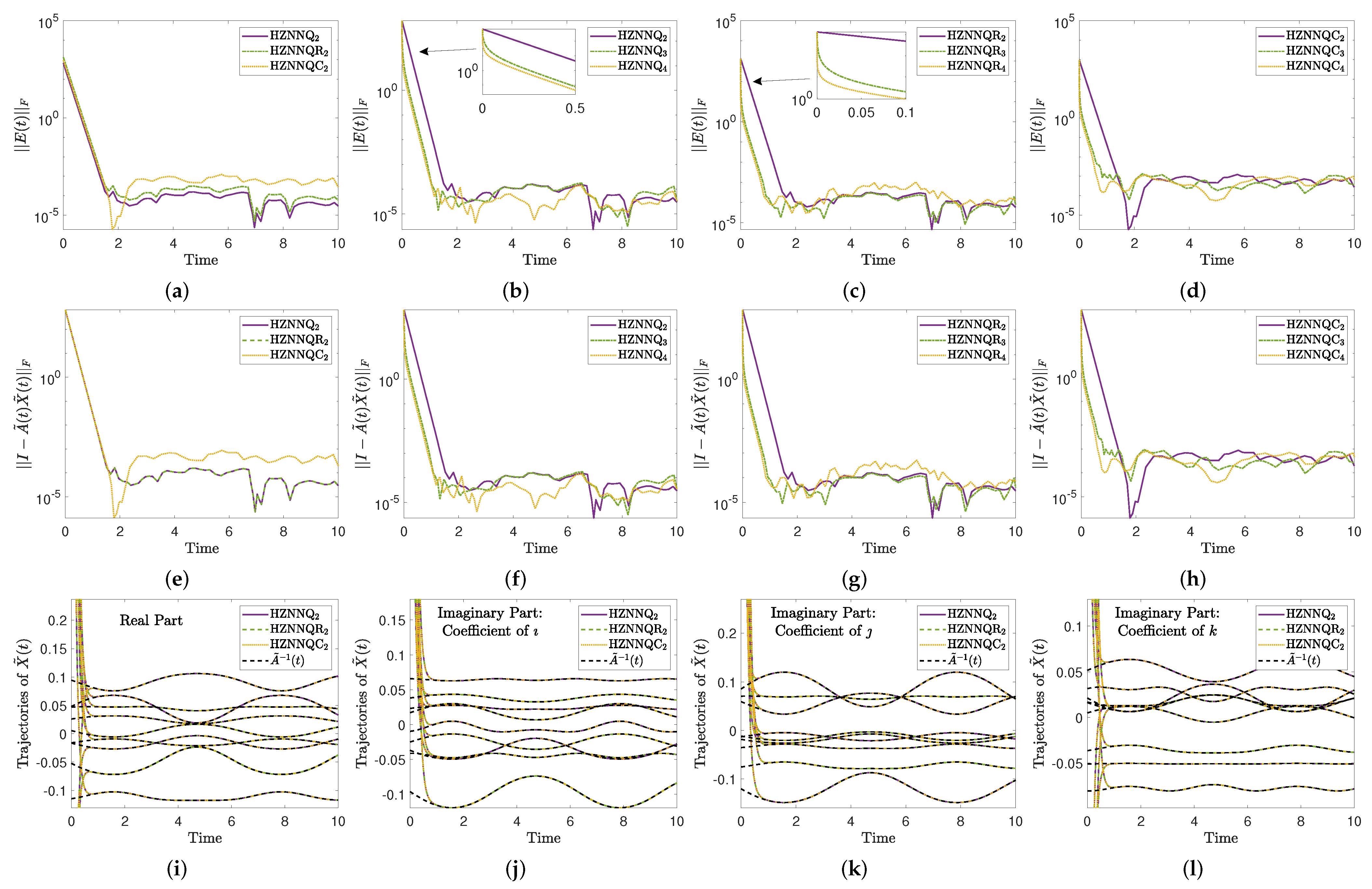
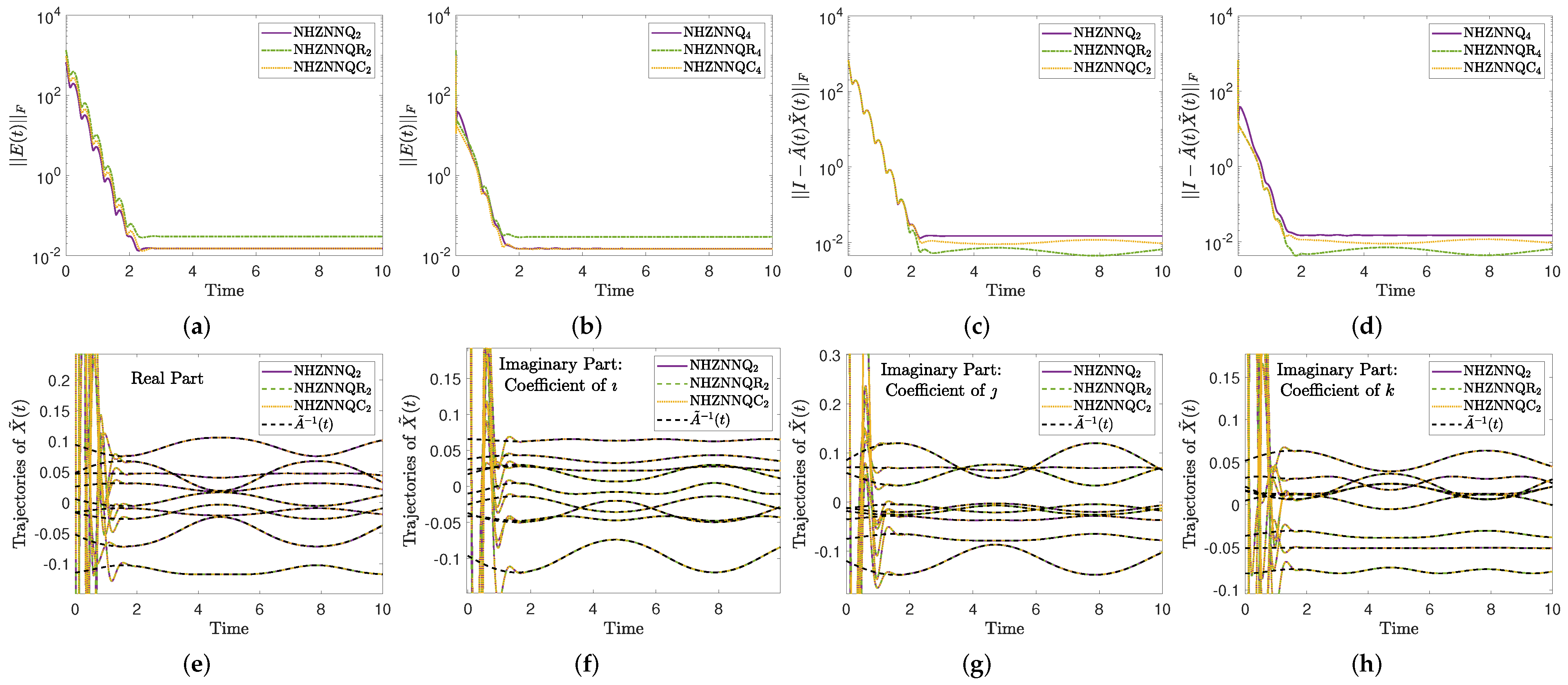
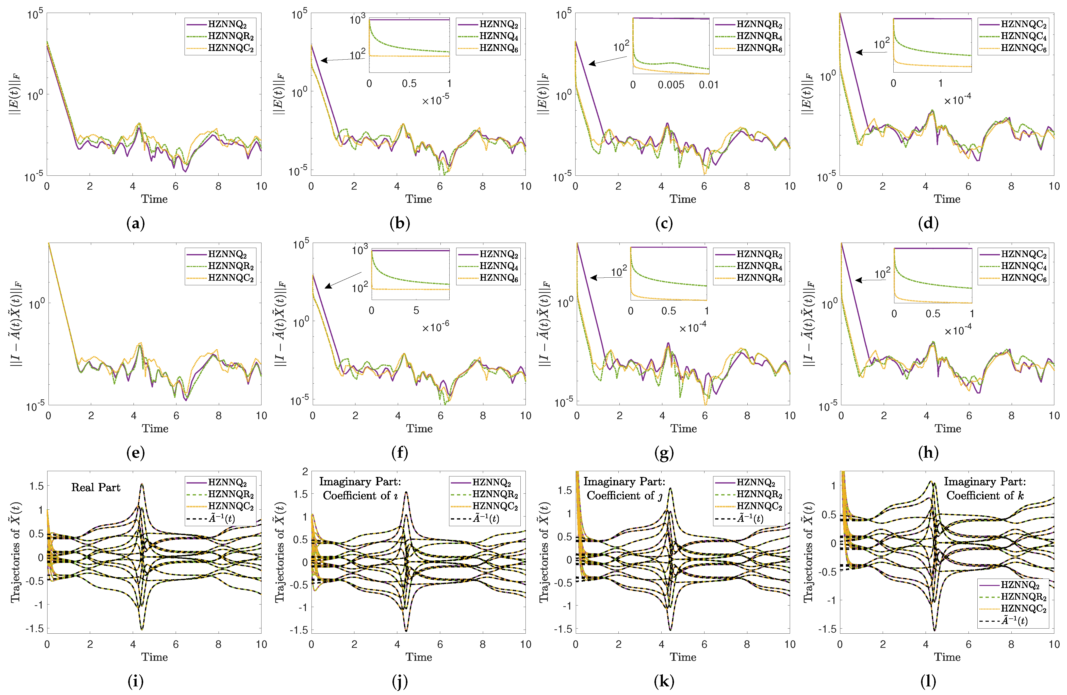
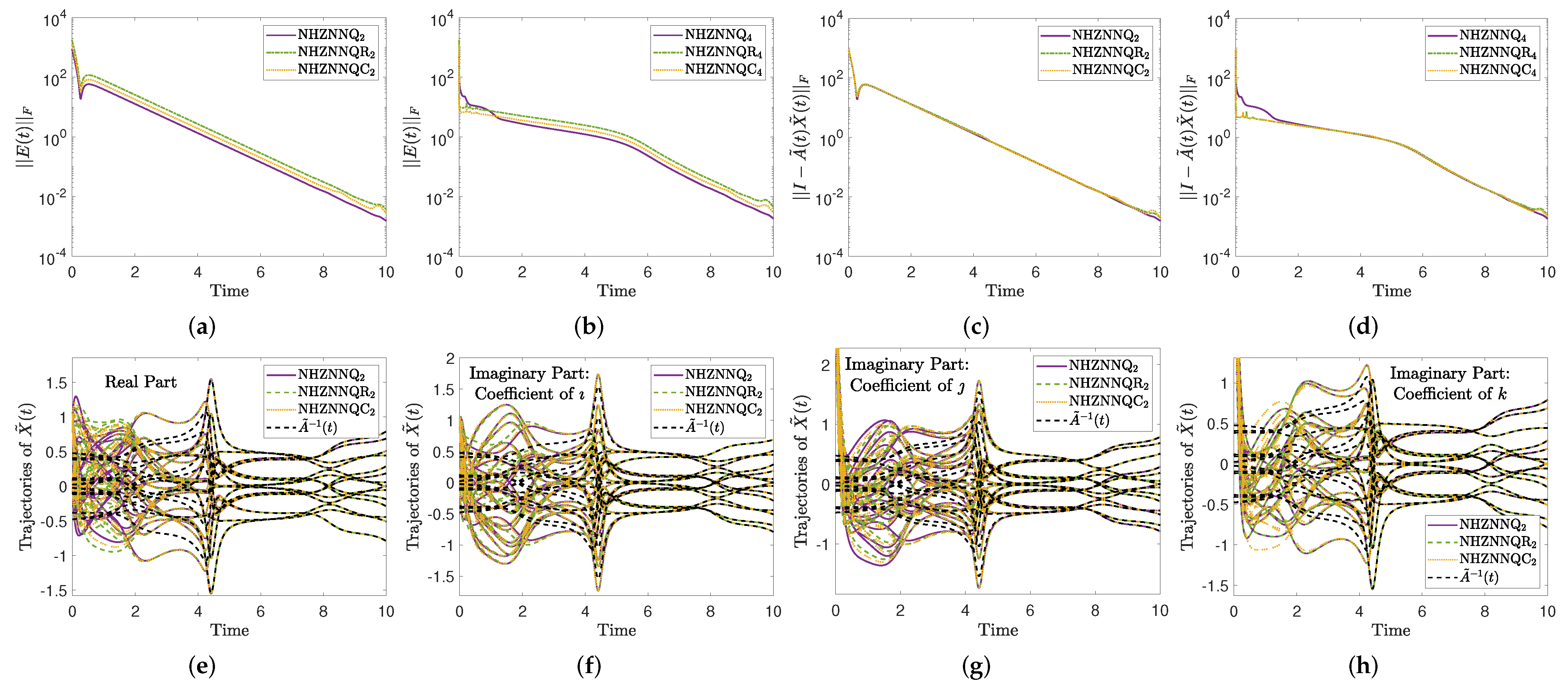
4. Computational Simulations

We will present two simulation examples (SEs) and one application to robotic motion tracking in this section. What follows are a few crucial explanations. The HZNN design parameter $\lambda$ is applied with value 10 in all SEs and with value 100 in the application. The starting points of the HZNNQ${}_p$, HZNNQC${}_p$, and HZNNQR${}_p$ models have been set to $\mathbf{y}\left(0\right)=\mathrm{vec}\left({[A_1^{\mathrm{T}}\left(0\right),A_2^{\mathrm{T}}\left(0\right),A_3^{\mathrm{T}}\left(0\right),A_4^{\mathrm{T}}\left(0\right)]}^{\mathrm{T}}\right)$, $\mathbf{k}\left(0\right)=\mathrm{vec}\left(\check{A}\right)$ and $\mathbf{x}\left(0\right)=\mathrm{vec}\left(A\right)$, respectively, and the starting points of the NHZNNQ${}_p$, NHZNNQC${}_p$, and NHZNNQR${}_p$ models have been set to ${\mathbf{y}}_N\left(0\right)=\mathrm{vec}\left({[{\mathbf{y}}^{\mathrm{T}}\left(0\right),{\mathbf{y}}^{\mathrm{T}}\left(0\right)]}^{\mathrm{T}}\right)$, ${\mathbf{k}}_N\left(0\right)=\mathrm{vec}\left({[{\mathbf{k}}^{\mathrm{T}}\left(0\right),{\mathbf{k}}^{\mathrm{T}}\left(0\right)]}^{\mathrm{T}}\right)$ and ${\mathbf{x}}_N\left(0\right)=\mathrm{vec}\left({[{\mathbf{x}}^{\mathrm{T}}\left(0\right),{\mathbf{x}}^{\mathrm{T}}\left(0\right)]}^{\mathrm{T}}\right)$, respectively. For convenience purposes, we have set $\beta \left(t\right)=cos\left(t\right)$ and $\alpha \left(t\right)=sin\left(t\right)$. Further, the noises used are the next:

• $N\left(t\right)=10·{\mathbf{1}}_{\rho }$ represents the constant noise;
• $N\left(t\right)=(2+t/4)·{\mathbf{1}}_{\rho }$ represents the linear noise;
• $N\left(t\right)=2+\alpha \left(t\right)·{\mathbf{1}}_{\rho }/4$ represents the bounded noise.

Finally, a MATLAB ode solver, to be specific ode15s, is used with the time interval being set to $[0,10]$ and $[0,20]$, respectively, in all SEs and the application. For this ode solver, the default double precision arithmetic ($eps=2.22\times {10}^{-16}$) is applied, causing the minimum value in each of the figures in this section to be primarily of the form ${10}^{-5}$.

4.1. Simulation Examples

4.1.1. Example 1

The following are the input matrix $\tilde{A}\left(t\right)$ coefficients:

$$\begin{gathered} A_1\left(t\right)=\left[\begin{array}{ccc}2\alpha \left(t\right)+2& -4& 4\\ 2\alpha \left(t\right)+6& -2& 6\\ 2\alpha \left(t\right)+7& -2& 4\end{array}\right],A_2\left(t\right)=\left[\begin{array}{ccc}6& 2\alpha \left(t\right)+1& 4\\ 5& 3\alpha \left(t\right)+1& 3\\ 5& 2\alpha \left(t\right)+2& 7\end{array}\right], \\ {A}_3\left(t\right)=\left[\begin{array}{ccc}3\alpha \left(t\right)+2& 9& 5\\ 2\alpha \left(t\right)+3& 12& 2\\ 3\alpha \left(t\right)+4& 3& 5\end{array}\right],A_4\left(t\right)=\left[\begin{array}{ccc}-2& \alpha \left(t\right)+1& 7\\ -4& 2\alpha \left(t\right)+4& 8\\ -2& 3\alpha \left(t\right)+1& 9\end{array}\right]. \end{gathered}$$

As a consequence, $\tilde{A}\left(t\right)\in {\mathbb{H}}^{3\times 3}$. The performance of the HZNN and NHZNN models is shown in Figure 1 and Figure 2.

4.1.2. Example 2

Considering the following matrix

$$K=\left[\begin{array}{ccccc}1& 1& 1& 1& 1\\ 0& 1& 1& 1& 1\\ 0& 0& 1& 1& 1\\ 0& 0& 0& 1& 1\\ 0& 0& 0& 0& 1\end{array}\right],$$

the following are the input matrix $\tilde{A}\left(t\right)$ coefficients:

$$\begin{array}{l}{A}_1\left(t\right)=K\odot (1+\alpha \left(t\right)),A_2\left(t\right)=K^{\mathrm{T}}\odot (1+2\alpha \left(t\right)),\\ A_3\left(t\right)=K\odot (1+3\beta \left(t\right)),A_4\left(t\right)=K^{\mathrm{T}}\odot (1+4\beta \left(t\right)).\end{array}$$

As a consequence, $\tilde{A}\left(t\right)\in {\mathbb{H}}^{5\times 5}$. The performance of the HZNN and NHZNN models is shown in Figure 3 and Figure 4.

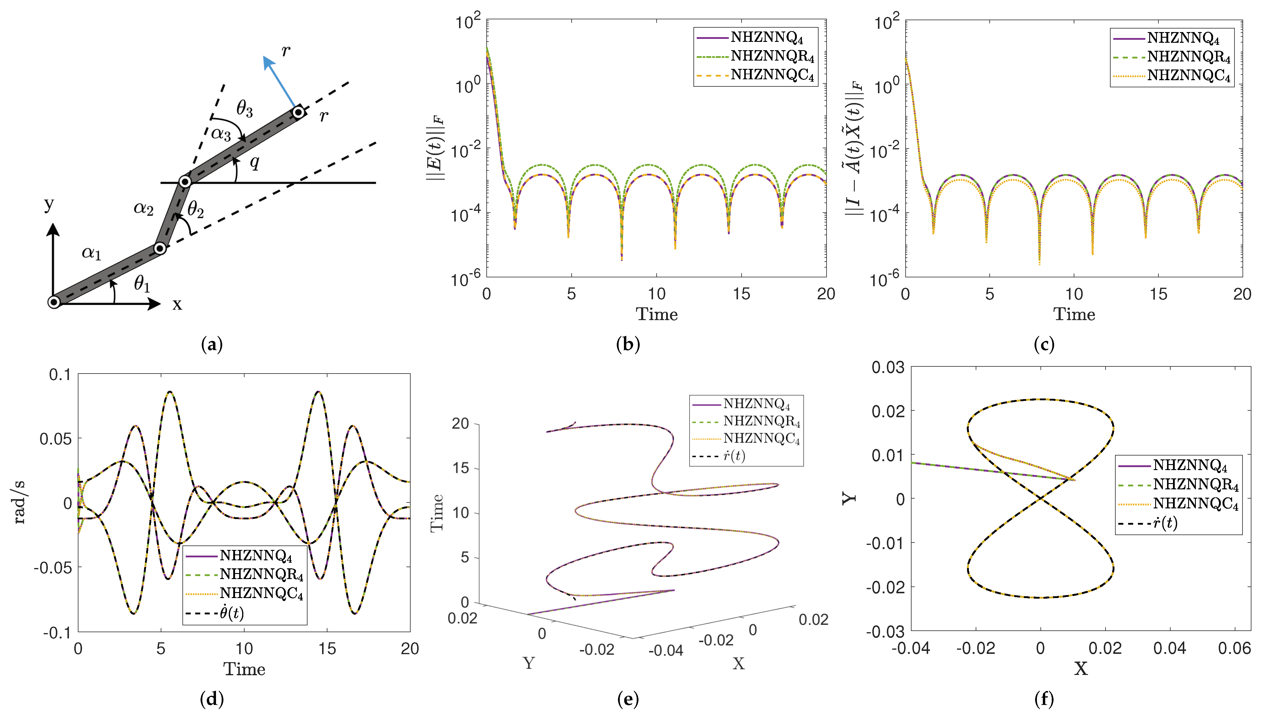
4.2. Application to Robotic Motion Tracking

The applicability of the NHZNNQ${}_p$, NHZNNQC${}_p$ and NHZNNQR${}_p$ models is validated in this experiment using a 3-link planar manipulator (PM), as shown in Figure 5a. It is important to mention that the 3-link PM’s kinematics equations at the position level $r\left(t\right)\in {\mathbb{R}}^n$ and the velocity level $\dot{r}\left(t\right)\in {\mathbb{R}}^n$ are expressed as follows:

$$r\left(t\right)=f\left(\theta \left(t\right)\right),\dot{r}\left(t\right)=J\left(\theta \right)\dot{\theta }\left(t\right),$$

(73)

where $\theta \in {\mathbb{R}}^n$ is the angle of the 3-link PM, $J\left(\theta \right)=\partial f\left(\theta \right)/\partial \theta \in {\mathbb{R}}^{n\times n}$, and $f(·)$ is a nonlinear smooth mapping function, $r\left(t\right)$ is the end effector’s position.

To comprehend how this 3-link PM tracked motion, the inverse kinematic equation is addressed. The equation of velocity can be thought of as a linear equations system when the end effector motion tracking task is assigned with $\dot{r}\left(t\right)$ known and $\dot{\theta }\left(t\right)$ unknown. To put it another way, by setting $\tilde{A}\left(t\right)=J\left(\theta \right)$, we find $\tilde{X}\left(t\right)=A^{-1}\left(t\right)$ to solve $\dot{\theta }\left(t\right)=\tilde{X}\left(t\right)\dot{r}\left(t\right)$. Therefore, we may track control of the 3-link PM by using the ZNN models to resolve the underlying linear equation system.

The 3-link PM’s end-effector is anticipated to follow a infinity-shaped path in the simulation experiment; Ref. [58] contains the X and Y-axis velocity functions of this path along with the specifications of 3-link PM. Additionally, the link length is $\alpha ={[1,2/3,5/4]}^{\mathrm{T}}$ and the initial value of the joints is $\theta \left(0\right)={[\pi /8,\pi /8,\pi /8]}^{\mathrm{T}}$. The performance of the NHZNN models under the bounded noise is shown in Figure 5.

4.3. Results and Discussion

The performance of the HZNNQ${}_p$ (23), HZNNQC${}_p$ (40), HZNNQR${}_p$ (57), NHZNNQ${}_p$ (28), NHZNNQC${}_p$ (45) and NHZNNQR${}_p$ (62) models for solving the TVQ-INV (8) is examined by the SEs in Section 4.1.1 and Section 4.1.2. A unique TVQ-INV problem, described by the proper TVQ matrix $\tilde{A}\left(t\right)$, is assigned to each section.

For the SE in Section 4.1.1, the results of the HZNNQ${}_p$, HZNNQC${}_p$, and HZNNQR${}_p$ models with input TVQ matrix $\tilde{A}\left(t\right)\in {\mathbb{H}}^{3\times 3}$ are presented in Figure 1. Particularly, Figure 1a–d depict the Frobenius norm of the models’ EMEs under $p=2,3,4$. In the case of $p=2$, we observe that, by the time-mark of $t\approx 2$, the models’ EMEs converge to the range $[{10}^{-5},{10}^{-3}]$. The time-mark, however, gets shorter as p’s value grows. The Frobenius norm of the model’s EMEs values, shown in

Table 1. Frobenius norm of the HZNN and NHZNN models’ EMEs in SEs of Section 4.1.1 and Section 4.1.2.

Model	SE of Section 4.1.1					SE of Section 4.1.2
	$\mathit{p}$	$\mathit{t}=\mathbf{0}$	$\mathit{t}={\mathbf{10}}^{-\mathbf{6}}$	$\mathit{t}={\mathbf{10}}^{-\mathbf{3}}$	$\mathit{t}={\mathbf{10}}^{-\mathbf{1}}$	$\mathit{p}$	$\mathit{t}=\mathbf{0}$	$\mathit{t}={\mathbf{10}}^{-\mathbf{6}}$	$\mathit{t}={\mathbf{10}}^{-\mathbf{3}}$	$\mathit{t}={\mathbf{10}}^{-\mathbf{1}}$
HZNNQ${}_p$	2	663.7	663.7	657.3	244.2	2	876.2	876.2	867.5	322.8
	3	663.7	661.8	288.1	6.6	4	876.2	236.3	79.1	22.1
	4	663.7	461.7	78.6	3.1	6	876.2	83.5	68.4	20.1
HZNNQC${}_p$	2	1327.4	1327.4	1314.5	488.5	2	1752.5	1752.5	1735.1	645.1
	3	1327.4	1321.5	212.3	1.9	4	1752.5	439.2	16.8	1.7
	4	1327.4	512.4	23.4	0.9	6	1752.5	26.7	8.6	1.5
HZNNQR${}_p$	2	938.6	938.6	929.5	345.1	2	1239.2	1239.2	1227.1	455.6
	3	938.6	934.5	150.2	1.3	4	1239.2	310.7	11.8	1.2
	4	938.6	362.7	16.5	0.6	6	1239.2	18.8	6.1	1.1
NHZNNQ${}_p$	2	663.7	663.7	657.9	199.9	2	876.2	876.2	867.6	304.2
	4	663.7	461.6	76.9	34.9	4	876.2	236.3	79.1	24.5
NHZNNQR${}_p$	2	1327.4	1327.4	1315.8	400.7	2	1752.5	1752.5	1735.2	610.1
	4	1327.4	512.5	21.3	18.5	4	1752.5	439.2	16.3	9.3
NHZNNQR${}_p$	2	938.6	938.6	930.4	285.4	2	1239.2	1239.2	1227.1	432.8
	4	938.6	362.3	15.1	13.1	4	1239.2	310.8	11.5	6.6

, likewise supports the aforementioned finding. The Frobenius norm of (8) in Figure 1e–h further supports this tendency. A higher price for $\lambda$ will typically push the HZNN models to converge even more quickly. The fact that all models successfully converged is emphasized once more in Figure 1i–l, where the theoretical trajectories of the real and imaginary parts of the TVQ matrix ${\tilde{A}}^{-1}\left(t\right)$ are contrasted with the $\tilde{X}\left(t\right)$ trajectories retrieved by the three models. On the other hand, the results of the NHZNNQ${}_p$, NHZNNQC${}_p$, and NHZNNQR${}_p$ models under the linear noise with $z=100$ are presented in Figure 2. Particularly, Figure 2a,b depict the Frobenius norm of the models’ EMEs under $p=2$ and $p=4$, respectively, and Figure 2c,d depict the Frobenius norm of (8) under $p=2$ and $p=4$, respectively. We note that the errors of the models converge to the range $[{10}^{-2},{10}^{-1}]$ by the time-mark of $t\approx 2$ in the case of $p=2$ and the time-mark of $t\approx 1.5$ in the case of $p=4$. That is, the time-mark gets shorter as p’s value grows. The fact that all models successfully converged is emphasized once more in Figure 2e–h, where the theoretical trajectories of the real and imaginary parts of the TVQ matrix ${\tilde{A}}^{-1}\left(t\right)$ are contrasted with the $\tilde{X}\left(t\right)$ trajectories retrieved by the three models.

For the SE in Section 4.1.2, the results of the HZNNQ${}_p$, HZNNQC${}_p$, and HZNNQR${}_p$ models with input TVQ matrix $\tilde{A}\left(t\right)\in {\mathbb{H}}^{5\times 5}$ are presented in Figure 3. Particularly, Figure 3a–d depict the Frobenius norm of the models’ EMEs under $p=2,4,6$. In the case of $p=2$, we observe that, by the time-mark of $t\approx 1.8$, the models’ EMEs converge to the range $[{10}^{-5},{10}^{-3}]$. The time-mark, however, gets shorter as p’s value grows. The EMEs’ Frobenius norm values of the models, as shown in Table 1, can be used to confirm the aforementioned result. The Frobenius norm of (8) in Figure 3e–h further supports this tendency. The fact that all models successfully converged is emphasized once more in Figure 3i–l, where the theoretical trajectories of the real and imaginary parts of the TVQ matrix ${\tilde{A}}^{-1}\left(t\right)$ are contrasted with the $\tilde{X}\left(t\right)$ trajectories retrieved by the three models. On the other hand, the results of the NHZNNQ${}_p$, NHZNNQC${}_p$, and NHZNNQR${}_p$ models under the constant noise with $z=10$ are presented in Figure 4. Particularly, Figure 4a,b depict the Frobenius norm of the models’ EMEs under $p=2$ and $p=4$, respectively, and Figure 4c,d depict the Frobenius norm of (8) under $p=2$ and $p=4$, respectively. We note that the errors of the models converge to the range $[{10}^{-3},{10}^{-2}]$ by the time-mark of $t\approx 10$ in both cases of $p=2$ and $p=4$. In contrast to $p=2$, the errors of the models converge slightly more quickly when $p=4$ in the time-range $[0,5]$. In other words, when p’s value increases, the pace of convergence increases in the time-range $[0,5]$. The fact that all models successfully converged is emphasized once more in Figure 4e–h, where the theoretical trajectories of the real and imaginary parts of the TVQ matrix ${\tilde{A}}^{-1}\left(t\right)$ are contrasted with the $\tilde{X}\left(t\right)$ trajectories retrieved by the three models.

For the application in Section 4.2, the results of the NHZNNQ${}_p$, NHZNNQC${}_p$, and NHZNNQR${}_p$ models under the bounded noise with $z=1000$ are presented in Figure 5. Particularly, Figure 5b,c depict the Frobenius norms of the models’ EMEs and (8) under $p=4$, respectively. We note that the errors of the models converge to the range $[{10}^{-5},{10}^{-2}]$ by the time-mark of $t\approx 1.5$. The fact that all models successfully converged is emphasized once more in Figure 5d–f, which depict the trajectories of the velocity and the infinity-shaped path tracking. As seen in these figures, all NHZNN model solutions match the actual velocity $\dot{\theta }\left(t\right)$, and the 3-link PM successfully completes the infinity-shaped path tracking task, where $\dot{r}\left(t\right)$ is the actual infinity-shaped path.

Lastly, once we take into account the complexity of each model, the results above can be placed into better context. Particularly, the HZNNQ${}_p$ model performs $4n^2$ additions/subtractions and ${\left(4n^2\right)}^2$ multiplications in each iteration of (23), which results in a computational complexity of $\mathcal{O}\left({\left(4n^2\right)}^3\right)$ when an ode MATLAB solver is used. In the same manner, the HZNNQC${}_p$ model performs $4n^2$ additions/subtractions and ${\left(4n^2\right)}^2$ multiplications in each iteration of (40). By converting these measurements from the complex domain into the real domain, the HZNNQC${}_p$ model performs $8n^2$ additions/subtractions and ${\left(8n^2\right)}^2$ multiplications, which results in a computational complexity of $\mathcal{O}\left({\left(8n^2\right)}^3\right)$. The HZNNQR${}_p$ model performs $16n^2$ additions/subtractions and ${\left(16n^2\right)}^2$ multiplications in each iteration of (57), which results in a computational complexity of $\mathcal{O}\left({\left(16n^2\right)}^3\right)$. The NHZNNQ${}_p$ model performs $8n^2$ additions/subtractions and ${\left(8n^2\right)}^2$ multiplications in each iteration of (28), which results in a computational complexity of $\mathcal{O}\left({\left(8n^2\right)}^3\right)$. The NHZNNQC${}_p$ model performs $8n^2$ additions/subtractions and ${\left(8n^2\right)}^2$ multiplications in each iteration of (45). Converting these measurements from the complex domain into the real domain, the NHZNNQC${}_p$ model performs $16n^2$ additions/subtractions and ${\left(16n^2\right)}^2$ multiplications which results in a computational complexity of $\mathcal{O}\left({\left(16n^2\right)}^3\right)$. The NHZNNQR${}_p$ model performs $32n^2$ additions/subtractions and ${\left(32n^2\right)}^2$ multiplications in each iteration of (62), which results in a computational complexity of $\mathcal{O}\left({\left(32n^2\right)}^3\right)$. Because the dimensions of the associated real valued matrix $A\left(t\right)$ are two times larger than those of the complex valued matrix $\check{A}\left(t\right)$ and four times larger than those of the quaternion valued matrix $\tilde{A}\left(t\right)$, the HZNNQR${}_p$ and NHZNNQR${}_p$ are, by far, the most complex models. Because of this, choosing to address the TVQ-INV problem in the real domain has a significant memory penalty, with RAM fast being a limiting factor as $\tilde{A}\left(t\right)$ grows in size. All six ZNN models can solve the TVQ-INV problem when all factors are considered, however the HZNNQ${}_p$ seems to have the most potential in the absence of noise, and the NHZNNQ${}_p$ seems to have the most promise in the presence of noise.

5. Conclusions

In view of handling the TVQ-INV problem, three models based on the HZNN design, namely HZNNQ${}_p$, HZNNQC${}_p$, and HZNNQR${}_p$, and three models based on the NHZNN design, namely NHZNNQ${}_p$, NHZNNQC${}_p$, and NHZNNQR${}_p$, have been proposed. Along with SEs and a practical application to Robotic motion tracking, the theoretical investigation has aided the creation of those models. Both direct and indirect approaches to solving the TVQ-INV problem—representing the results in the complex and real domains before converting the results back to the quaternion domain—have proved effective. Of the two approaches, the direct method, used by the HZNNQ${}_p$ and NHZNNQ${}_p$ models, has been suggested as the most effective and efficient. That is, according to the principal results, each of these six models can solve the TVQ-INV effectively, and the HZNN strategy offers a faster convergence rate than the conventional ZNN strategy. In light of this, the established findings pave the path for more engaging research projects. Here are a few topics to consider for future studies:

• One may look at using nonlinear ZNNs for time-varying quaternion issues;
• It is possible to investigate using the finite-time ZNN framework to time-varying quaternion problems.

References

1. Ben-Israel, A.; Greville, T.N.E. Generalized Inverses: Theory and Applications, 2nd ed.; CMS Books in Mathematics; Springer: New York, NY, USA, 2003. [Google Scholar] [CrossRef]
2. Wang, G.; Wei, Y.; Qiao, S.; Lin, P.; Chen, Y. Generalized Inverses: Theory and Computations; Springer: Singapore, 2018; Volume 53. [Google Scholar]
3. Zhang, S.; Dong, Y.; Ouyang, Y.; Yin, Z.; Peng, K. Adaptive neural control for robotic manipulators with output constraints and uncertainties. IEEE Trans. Neural Netw. Learn. Syst. 2018, 29, 5554–5564. [Google Scholar] [CrossRef] [PubMed]
4. Yuan, Y.; Wang, Z.; Guo, L. Event-triggered strategy design for discrete-time nonlinear quadratic games with disturbance compensations: The noncooperative case. IEEE Trans. Syst. Man Cybern. Syst. 2018, 48, 1885–1896. [Google Scholar] [CrossRef]
5. Mourtas, S.D.; Katsikis, V.N.; Kasimis, C. Feedback control systems stabilization using a bio-inspired neural network. EAI Endorsed Trans. AI Robots 2022, 1, 1–13. [Google Scholar] [CrossRef]
6. Yang, X.; He, H. Self-learning robust optimal control for continuous-time nonlinear systems with mismatched disturbances. Neural Netw. 2018, 99, 19–30. [Google Scholar] [CrossRef] [PubMed]
7. Li, S.; He, J.; Li, Y.; Rafique, M.U. Distributed recurrent neural networks for cooperative control of manipulators: A game-theoretic perspective. IEEE Trans. Neural Netw. Learn. Syst. 2017, 28, 415–426. [Google Scholar] [CrossRef] [PubMed]
8. Mourtas, S.D. A weights direct determination neuronet for time-series with applications in the industrial indices of the federal reserve bank of St. Louis. J. Forecast. 2022, 14, 1512–1524. [Google Scholar] [CrossRef]
9. Joldeş, M.; Muller, J.M. Algorithms for manipulating quaternions in floating-point arithmetic. In Proceedings of the 2020 IEEE 27th Symposium on Computer Arithmetic (ARITH), Portland, OR, USA, 7–10 June 2020; pp. 48–55. [Google Scholar]
10. Szynal-Liana, A.; Włoch, I. Generalized commutative quaternions of the Fibonacci type. Boletín Soc. Mat. Mex. 2022, 28, 1. [Google Scholar] [CrossRef]
11. Pavllo, D.; Feichtenhofer, C.; Auli, M.; Grangier, D. Modeling human motion with quaternion-based neural networks. Int. J. Comput. Vis. 2020, 128, 855–872. [Google Scholar] [CrossRef] [Green Version]
12. Özgür, E.; Mezouar, Y. Kinematic modeling and control of a robot arm using unit dual quaternions. Robot. Auton. Syst. 2016, 77, 66–73. [Google Scholar] [CrossRef]
13. Du, G.; Liang, Y.; Gao, B.; Otaibi, S.A.; Li, D. A cognitive joint angle compensation system based on self-feedback fuzzy neural network with incremental learning. IEEE Trans. Ind. Inform. 2021, 17, 2928–2937. [Google Scholar] [CrossRef]
14. Goodyear, A.M.S.; Singla, P.; Spencer, D.B. Analytical state transition matrix for dual-quaternions for spacecraft pose estimation. In Proceedings of the AAS/AIAA Astrodynamics Specialist Conference, Portland, ME, USA, 11–15 August 2019; Univelt Inc.: Escondido, CA, USA, 2020; pp. 393–411. [Google Scholar]
15. Giardino, S. Quaternionic quantum mechanics in real Hilbert space. J. Geom. Phys. 2020, 158, 103956. [Google Scholar] [CrossRef]
16. Kansu, M.E. Quaternionic representation of electromagnetism for material media. Int. J. Geom. Methods Mod. Phys. 2019, 16, 1950105. [Google Scholar] [CrossRef]
17. Weng, Z.H. Field equations in the complex quaternion spaces. Adv. Math. Phys. 2014, 2014, 450262. [Google Scholar] [CrossRef] [Green Version]
18. Ghiloni, R.; Moretti, V.; Perotti, A. Continuous slice functional calculus in quaternionic Hilbert spaces. Rev. Math. Phys. 2013, 25, 1350006. [Google Scholar] [CrossRef]
19. Kyrchei, I.I.; Mosić, D.; Stanimirović, P.S. MPCEP-*CEPMP-solutions of some restricted quaternion matrix equations. Adv. Appl. Clifford Algebr. 2022, 32, 22. [Google Scholar] [CrossRef]
20. Huang, L.; Wang, Q.W.; Zhang, Y. The Moore-Penrose inverses of matrices over quaternion polynomial rings. Linear Algebra Its Appl. 2015, 475, 45–61. [Google Scholar] [CrossRef]
21. Xiao, L.; Liu, S.; Wang, X.; He, Y.; Jia, L.; Xu, Y. Zeroing neural networks for dynamic quaternion-valued matrix inversion. IEEE Trans. Ind. Inform. 2022, 18, 1562–1571. [Google Scholar] [CrossRef]
22. Xiao, L.; Huang, W.; Li, X.; Sun, F.; Liao, Q.; Jia, L.; Li, J.; Liu, S. ZNNs with a varying-parameter design formula for dynamic Sylvester quaternion matrix equation. IEEE Trans. Neural Netw. Learn. Syst. 2022, 1–11. [Google Scholar] [CrossRef]
23. Xiao, L.; Cao, P.; Song, W.; Luo, L.; Tang, W. A fixed-time noise-tolerance ZNN model for time-variant inequality-constrained quaternion matrix least-squares problem. IEEE Trans. Neural Netw. Learn. Syst. 2023, 1–10. [Google Scholar] [CrossRef]
24. Xiao, L.; Zhang, Y.; Huang, W.; Jia, L.; Gao, X. A dynamic parameter noise-tolerant zeroing neural network for time-varying quaternion matrix equation with applications. IEEE Trans. Neural Netw. Learn. Syst. 2022, 1–10. [Google Scholar] [CrossRef]
25. Tan, N.; Yu, P.; Ni, F. New varying-parameter recursive neural networks for model-free kinematic control of redundant manipulators with limited measurements. IEEE Trans. Instrum. Meas. 2022, 71, 1–14. [Google Scholar] [CrossRef]
26. Dachang, Z.; Aodong, C.; Baolin, D.; Puchen, Z. Dual-mode synchronization predictive control of robotic manipulator. J. Dyn. Syst. Meas. Control 2022, 144, 111002. [Google Scholar] [CrossRef]
27. Jerbi, H.; Al-Darraji, I.; Tsaramirsis, G.; Ladhar, L.; Omri, M. Hamilton-Jacobi inequality adaptive robust learning tracking controller of wearable robotic knee system. Mathematics 2023, 11, 1351. [Google Scholar] [CrossRef]
28. Zhang, Y.; Ge, S.S. Design and analysis of a general recurrent neural network model for time-varying matrix inversion. IEEE Trans. Neural Netw. 2005, 16, 1477–1490. [Google Scholar] [CrossRef] [Green Version]
29. Chai, Y.; Li, H.; Qiao, D.; Qin, S.; Feng, J. A neural network for Moore-Penrose inverse of time-varying complex-valued matrices. Int. J. Comput. Intell. Syst. 2020, 13, 663–671. [Google Scholar] [CrossRef]
30. Sun, Z.; Li, F.; Jin, L.; Shi, T.; Liu, K. Noise-tolerant neural algorithm for online solving time-varying full-rank matrix Moore-Penrose inverse problems: A control-theoretic approach. Neurocomputing 2020, 413, 158–172. [Google Scholar] [CrossRef]
31. Wu, W.; Zheng, B. Improved recurrent neural networks for solving Moore-Penrose inverse of real-time full-rank matrix. Neurocomputing 2020, 418, 221–231. [Google Scholar] [CrossRef]
32. Zhang, Y.; Yang, Y.; Tan, N.; Cai, B. Zhang neural network solving for time-varying full-rank matrix Moore-Penrose inverse. Computing 2011, 92, 97–121. [Google Scholar] [CrossRef]
33. Qiao, S.; Wang, X.Z.; Wei, Y. Two finite-time convergent Zhang neural network models for time-varying complex matrix Drazin inverse. Linear Algebra Its Appl. 2018, 542, 101–117. [Google Scholar] [CrossRef]
34. Qiao, S.; Wei, Y.; Zhang, X. Computing time-varying ML-weighted pseudoinverse by the Zhang neural networks. Numer. Funct. Anal. Optim. 2020, 41, 1672–1693. [Google Scholar] [CrossRef]
35. Wang, X.; Stanimirovic, P.S.; Wei, Y. Complex ZFs for computing time-varying complex outer inverses. Neurocomputing 2018, 275, 983–1001. [Google Scholar] [CrossRef]
36. Simos, T.E.; Katsikis, V.N.; Mourtas, S.D.; Stanimirović, P.S.; Gerontitis, D. A higher-order zeroing neural network for pseudoinversion of an arbitrary time-varying matrix with applications to mobile object localization. Inf. Sci. 2022, 600, 226–238. [Google Scholar] [CrossRef]
37. Zhou, M.; Chen, J.; Stanimirovic, P.S.; Katsikis, V.N.; Ma, H. Complex varying-parameter Zhang neural networks for computing core and core-EP inverse. Neural Process. Lett. 2020, 51, 1299–1329. [Google Scholar] [CrossRef]
38. Kovalnogov, V.N.; Fedorov, R.V.; Generalov, D.A.; Chukalin, A.V.; Katsikis, V.N.; Mourtas, S.D.; Simos, T.E. Portfolio insurance through error-correction neural networks. Mathematics 2022, 10, 3335. [Google Scholar] [CrossRef]
39. Mourtas, S.D.; Katsikis, V.N. Exploiting the Black-Litterman framework through error-correction neural networks. Neurocomputing 2022, 498, 43–58. [Google Scholar] [CrossRef]
40. Mourtas, S.D.; Kasimis, C. Exploiting mean-variance portfolio optimization problems through zeroing neural networks. Mathematics 2022, 10, 3079. [Google Scholar] [CrossRef]
41. Jiang, W.; Lin, C.L.; Katsikis, V.N.; Mourtas, S.D.; Stanimirović, P.S.; Simos, T.E. Zeroing neural network approaches based on direct and indirect methods for solving the Yang–Baxter-like matrix equation. Mathematics 2022, 10, 1950. [Google Scholar] [CrossRef]
42. Katsikis, V.N.; Mourtas, S.D.; Stanimirović, P.S.; Zhang, Y. Continuous-time varying complex QR decomposition via zeroing neural dynamics. Neural Process. Lett. 2021, 53, 3573–3590. [Google Scholar] [CrossRef]
43. Stanimirović, P.S.; Katsikis, V.N.; Li, S. Higher-order ZNN dynamics. Neural Process. Lett. 2019, 51, 697–721. [Google Scholar] [CrossRef]
44. Kornilova, M.; Kovalnogov, V.; Fedorov, R.; Zamaleev, M.; Katsikis, V.N.; Mourtas, S.D.; Simos, T.E. Zeroing neural network for pseudoinversion of an arbitrary time-varying matrix based on singular value decomposition. Mathematics 2022, 10, 1208. [Google Scholar] [CrossRef]
45. Dai, J.; Tan, P.; Yang, X.; Xiao, L.; Jia, L.; He, Y. A fuzzy adaptive zeroing neural network with superior finite-time convergence for solving time-variant linear matrix equations. Knowl.-Based Syst. 2022, 242, 108405. [Google Scholar] [CrossRef]
46. Xiao, L.; Tan, H.; Dai, J.; Jia, L.; Tang, W. High-order error function designs to compute time-varying linear matrix equations. Inf. Sci. 2021, 576, 173–186. [Google Scholar] [CrossRef]
47. Zhong, N.; Huang, Q.; Yang, S.; Ouyang, F.; Zhang, Z. A varying-parameter recurrent neural network combined with penalty function for solving constrained multi-criteria optimization scheme for redundant robot manipulators. IEEE Access 2021, 9, 50810–50818. [Google Scholar] [CrossRef]
48. Climent, J.; Thome, N.; Wei, Y. A geometrical approach on generalized inverses by Neumann-type series. Linear Algebra Appl. 2001, 332–334, 533–540. [Google Scholar] [CrossRef] [Green Version]
49. Li, W.; Li, Z. A family of iterative methods for computing the approximate inverse of a square matrix and inner inverse of a non-square matrix. Appl. Math. Comput. 2010, 215, 3433–3442. [Google Scholar] [CrossRef]
50. Liu, X.; Jin, H.; Yu, Y. Higher-order convergent iterative method for computing the generalized inverse and its application to Toeplitz matrices. Linear Algebra Appl. 2013, 439, 1635–1650. [Google Scholar] [CrossRef]
51. Weiguo, L.; Juan, L.; Tiantian, Q. A family of iterative methods for computing Moore-Penrose inverse of a matrix. Linear Algebra Appl. 2013, 438, 47–56. [Google Scholar] [CrossRef]
52. Stanimirović, P.S.; Srivastava, S.; Gupta, D.K. From Zhang Neural Network to scaled hyperpower iterations. J. Comput. Appl. Math. 2018, 331, 133–155. [Google Scholar] [CrossRef]
53. Katsikis, V.N.; Stanimirović, P.S.; Mourtas, S.D.; Li, S.; Cao, X. Chapter Towards higher order dynamical systems. In Generalized Inverses: Algorithms and Applications; Mathematics Research Developments; Nova Science Publishers, Inc.: New York, NY, USA, 2021; pp. 207–239. [Google Scholar]
54. Jin, L.; Zhang, Y.; Li, S. Integration-Enhanced Zhang Neural Network for Real-Time-Varying Matrix Inversion in the Presence of Various Kinds of Noises. IEEE Trans. Neural Netw. Learn. Syst. 2016, 27, 2615–2627. [Google Scholar] [CrossRef]
55. Farebrother, R.W.; Groß, J.; Troschke, S.O. Matrix representation of quaternions. Linear Algebra Its Appl. 2003, 362, 251–255. [Google Scholar] [CrossRef] [Green Version]
56. Simos, T.E.; Katsikis, V.N.; Mourtas, S.D.; Stanimirović, P.S. Finite-time convergent zeroing neural network for solving time-varying algebraic Riccati equations. J. Frankl. Inst. 2022, 359, 10867–10883. [Google Scholar] [CrossRef]
57. Liu, H.; Wang, T.; Guo, D. Design and validation of zeroing neural network to solve time-varying algebraic Riccati equation. IEEE Access 2020, 8, 211315–211323. [Google Scholar] [CrossRef]
58. Zhang, Y.; Jin, L. Robot Manipulator Redundancy Resolution; John Wiley & Sons: Hoboken, NJ, USA, 2017. [Google Scholar] [CrossRef]
Figure 1. EMEs, error of (8), and the trajectories of X ˜ ( t ) in Section 4.1.1. (a) EMEs for p = 2 . (b) EMEs of HZNNQ p . (c) EMEs of HZNNQR p . (d) EMEs of HZNNQC p . (e) Error of (8) for p = 2 . (f) HZNNQ p error of (8). (g) HZNNQR p error of (8). (h) HZNNQC p error of (8). (i) Solutions traj. (j) Solutions traj. (k) Solutions traj. (l) Solutions traj.
Mathematics 11 02756 g001
Figure 2. EMEs, error of (8), and the trajectories of X ˜ ( t ) in Section 4.1.1 under linear noise with z = 100 . (a) EMEs for p = 2 . (b) EMEs for p = 4 . (c) Error of (8) for p = 2 . (d) Error of (8) for p = 4 . (e) Solutions traj. (f) Solutions traj. (g) Solutions traj. (h) Solutions traj.
Mathematics 11 02756 g002
Figure 3. EMEs, error of (8), and the trajectories of X ˜ ( t ) in Section 4.1.2. (a) EMEs for p = 2 . (b) EMEs of HZNNQ p . (c) EMEs of HZNNQR p . (d) EMEs of HZNNQC p . (e) Error of (8) for p = 2 . (f) HZNNQ p error of (8). (g) HZNNQR p error of (8). (h) HZNNQC p error of (8). (i) Solutions traj. (j) Solutions traj. (k) Solutions traj. (l) Solutions traj.
Mathematics 11 02756 g003
Figure 4. EMEs, error of (8), and the trajectories of X ˜ ( t ) in Section 4.1.2 under constant noise with z = 10 . (a) EMEs for p = 2 . (b) EMEs for p = 4 . (c) Error of (8) for p = 2 . (d) Error of (8) for p = 4 . (e) Solutions traj. (f) Solutions traj. (g) Solutions traj. (h) Solutions traj.
Mathematics 11 02756 g004
Figure 5. Robotic motion tracking application results under bounded noise with z = 1000 . (a) 3-link PM. (b) EMEs for p = 4 . (c) Error of (8). (d) Velocity. (e) Path tracking 3D. (f) Path tracking 2D.
Mathematics 11 02756 g005