Article

Surrogate-Based Physics-Informed Neural Networks for Elliptic Partial Differential Equations †

College of Civil Engineering, Tongji University, Shanghai 200092, China
*
Author to whom correspondence should be addressed.
This paper is an extended version of our paper published in 2022 15th World Congress on Computational Mechanics, Virtual Congress, 31 July–5 August 2022.
Mathematics 2023, 11(12), 2723; https://doi.org/10.3390/math11122723
Submission received: 19 May 2023 / Revised: 9 June 2023 / Accepted: 14 June 2023 / Published: 15 June 2023
(This article belongs to the Special Issue Advances in Applied Mathematics, Mechanics and Engineering)

Abstract

:
The purpose of this study is to investigate the role that a deep learning approach could play in computational mechanics. In this paper, a convolutional neural network technique based on modified loss function is proposed as a surrogate of the finite element method (FEM). Several surrogate-based physics-informed neural networks (PINNs) are developed to solve representative boundary value problems based on elliptic partial differential equations (PDEs). According to the authors’ knowledge, the proposed method has been applied for the first time to solve boundary value problems with elliptic partial differential equations as the governing equations. The results of the proposed surrogate-based approach are in good agreement with those of the conventional FEM. It is found that modification of the loss function could improve the prediction accuracy of the neural network. It is demonstrated that to some extent, the deep learning approach could replace the conventional numerical method as a significant surrogate model.

1. Introduction

In the initial stages of the widespread development of computers, they received widespread attention due to their computing power surpassing that of humans. This has also driven the development of various computational methods. The most well-known among them is the finite element method, one of the most effective methods for solving boundary value problems with partial differential equations as governing equations [1,2,3,4,5].
In recent years, however, the learning capability of computers has also been impressive in addition to computing power. The question of how to combine computational techniques with the learning abilities of computers has become a research focus in the academic community. For example, some scholars directly used the deep learning technique to solve boundary value problems [6,7]. These kinds of methods have several advantages. For instance, it has been found that the artificial neural network avoids the curse of dimensionality [8]. So-called computer learning ability is generated in the form of neural networks in which the most widely used networks were named the physical information neural networks (PINNs) proposed by Raissi et al. [9,10]. The PINNs have been applied to computational fluid and solid mechanics [11,12].
Based on PINNs, a variety of neural networks were developed to solve partial differential equations. Yang et al. [13] developed the Bayesian physics-informed neural network, B-PINN, which could use physical laws and noise measurements to solve forward and inverse nonlinear problems described by partial differential equations and noisy data. Leung et al. [14] proposed a neural homogenization-based physics-informed neural network, NH-PINN, which could solve multiscale problems with the help of homogenization. Furthermore, there were other PINNS, such as fractional PINNs (fPINNs) [15], nonlocal PINNs (nPINNs) [16], and extended PINNs (XPINNs) [17]. Haghighat et al. [18] combined momentum balance and constitutive relation with PINNs to solve the linear elastic problem of solid mechanics. Lu et al. [19] established the Python library for PINNs and DeepXDE as an analytical method for solving boundary value problems. Sirignano and Spiliopoulos [20] combined Galerkin methods and deep learning to solve high-dimensional free boundary partial differential equations, and the algorithm was meshfree because the mesh became infeasible for high-dimensional problems. Samaniego et al. [21] explored the variational formulation of PDEs and their corresponding functional which physically represents energy.
Another technique is well known as the data-based method. This approach had a wide range of applications. Finite element simulation could generate a large amount of data for training the neural network. After the neural network was trained, the calculation time could be saved. A trained neural network was equivalent to a surrogate model. Neural networks could directly compute approximate solutions within the range of a training set, but once the initial conditions and the parameters were changed, the neural network needed to be retrained.
Liang et al. [22] developed a deep learning model to directly estimate the stress distributions of the aorta, and the results were highly consistent with those from the FEM. Then, a general surrogate-based model was developed to analyze diverse structures, such as domes, walls, slabs, trusses, and frames. In the surrogate-based model, the features of structural components, including nodal points and elements, were used as input data and stress output data [23]. Next, more advanced techniques such as convolutional neural networks were used to predict the mechanical properties of two-dimensional checkerboard composites, where training data were generated from finite element analysis [24]. So-called surrogacy was originally a medical term that referred to the replacement of infertile women with fertile women. Here, it refers to using the finite element method to generate data to train a neural network model, thereby replacing the finite element method. For example, Nie et al. [25] have trained artificial neural networks using the results of two-dimensional finite element analyses to predict a stress field of cantilevered structures. Jiang et al. [26] have trained conditional generative adversarial networks to simulate complicated partial differential equations.
In addition, studies focused on investigating the role the artificial intelligence technique could play in numerical analysis were numerous, especially in past two years. For instance, the slope stability of soil was evaluated and predicted using machine learning techniques [27,28]. Furthermore, the deep learning neural network was used for damage detection and damage classification [29,30]. In addition, the estimation of the optimum design of structural systems was made using metaheuristic algorithms [31,32]. Furthermore, a digital image correlation based structural state and service life were detected using deep learning [33,34]. However, research exploring artificial intelligence techniques used as a surrogate for the finite element method is limited.
This study aimed to explore whether artificial intelligence techniques could be a qualified surrogate of the conventional numerical method or not. In this paper, a convolutional neural network technique based on modified loss function is proposed as a surrogate of the finite element method (FEM). Several surrogate-based physics-informed neural networks (PINNs) are developed to solve representative boundary value problems based on elliptic partial differential equations (PDEs). According to the authors’ knowledge, the proposed method has been applied for the first time to solve boundary value problems with elliptic partial differential equations as the governing equations. The results from the proposed surrogate-based approach are in good agreement with those from the conventional FEM. It is found that the modification of the loss function could improve the prediction precision of the neural network. It is demonstrated that to some extent, the deep learning approach could replace the conventional numerical method as a significant surrogate model.

2. Surrogate-Based Physics-Informed Neural Networks

2.1. Conventional Finite Element Method

In classical linear elasto-statics, a formal statement of the strong form of the boundary value problem goes as follows:
( S ) { Given   f i : Ω ,   g i : Γ g i ,   and   h i : Γ h i ,   find   u i : Ω ¯   such   that σ i j , j + f i = 0   in   Ω u i = g i   on   Γ g i σ i j n j = h i   on   Γ h i where   σ i j = c i j k l ε k l ,   ε k l = u ( k , l ) u k , l + u l . k 2 .
More definitions of notations are given as follows: i, j, k, and l are spatial indices, denotes the set of real numbers, Ω is the domain in , Γ is the boundary of Ω , Γ g i is part of the boundary where Dirichlet conditions are specified, Γ h i is part of the boundary where Neumann conditions are specified, δ are the collections of trail solutions, f i is the body force vector, g i is the prescribed boundary displacement vector, h i is the prescribed boundary traction vector, ε k l is the infinitesimal strain tensor, σ i j is the Cauchy stress tensor, and c i j k l are the elastic coefficients.
In classical linear elasto-statics, a formal statement of the weak form of the boundary value problem goes as follows:
( W ) { Given   f ,   g ,   and   h ,   in   which   f i : Ω ,   g i : Γ g i ,   and   h i : Γ h i ,   find   u δ   such   that   for   all   w V a ( w ,   u ) = ( w ,   f ) + ( w ,   h ) Γ where   a ( w ,   u ) = Ω w ( i , j ) c i j k l u ( k . l ) d Ω , ( w ,   f ) = Ω w i f i d Ω , ( w ,   h ) Γ = i = 1 n s d ( Γ h i w i h i d Γ ) .
More definitions of notations are given as follows: δ are the collections of trail solutions, u are the trial solutions, V are the collections of weighting functions, w are the weighting functions, f is the body force vector, g is the prescribed boundary displacement vector, and h is the prescribed boundary traction vector.
In classical linear elasto-statics, a formal statement of the Galerkin form of the boundary value problem goes as follows:
( G ) { Given   f ,   g ,   and   h ,   in   which   f i : Ω ,   g i : Γ g i ,   and   h i : Γ h i ,   find   u h = v h + g h δ h   such   that   for   all   w h V h a ( w h ,   v h ) = ( w h ,   f ) + ( w h ,   h ) Γ a ( w h ,   g h ) where   δ h   and   V h   are   finite - dimensional   approximations   to   δ   and   V , a ( w h ,   v h ) = Ω w h ( i , j ) c i j k l v h ( k . l ) d Ω ( w ,   f ) = Ω w i f i d Ω ( w h ,   h ) Γ = i = 1 n s d ( Γ h i w h i h i d Γ ) a ( w h ,   g h ) = Ω w h ( i , j ) c i j k l g h ( k . l ) d Ω
More definitions of notations are given as follows: h is the mesh parameter, δ h are the finite-dimensional collections of trail solutions, Vh are the finite-dimensional collections of weighting functions, uih, u h are the finite-dimensional trial solutions, wih, w h are the finite-dimensional weighting functions, g i h , and g h are extensions of the boundary displacement vector.

2.2. Artificial Neural Networks

After the artificial neural network was widely studied, the surrogate model was also widely developed and used in various fields. However, mathematical theories related to it are rare. At the same time, research on physical information neural networks is also in full swing. This article is based on the finite element theory and is derived from the mathematical expressions of data-driven proxy methods and physical information neural networks, respectively. In addition, the differences between the two methods are compared.
The artificial neural network is denoted as l = 1 L (α; W, b). Neural networks are based on the linear Gaussian regression process to fit the relationships between arrays. Through multilayer linear regression deep neural networks, extremely complex fitting relationships can be identified. In addition, such relationships are usually implicit, just like black boxes. Gaussian processes are among a class of methods known as kernel machines and are analogous to regularization approaches.
Let l = 1 L (α; W, b): d x d y be an L-layer neural network. This network is a feed-forward network, meaning that each layer creates data for the next layer through the following nested transformations:
h j = σ ( ω j i x i + b j )
y k = ω k j h j + b k
where ω j i , ω k j denote weights, b j , b k denote the biases, and σ denotes the activation function.
In this study, we use the multilayer perceptron, namely, the forward neural network (FNN), as the artificial neural network. The forward neural network has input, hidden, and output layers, where xi denotes the ith input data, hj denotes the jth hidden layer, and yk denotes the kth output data. Many of the most-used activation functions, including the relu function, sigmoid function, tanh function, and softplus function, are used in this study.

2.3. Surrogate-Based Physics-Informed Neural Networks (PINNs)

The surrogate-based approach is simply denoted as FEM l = 1 L . It is indicated that the finite element computational schemes are replaced by the trained learning neural networks. Let us take three-dimensional linear elastic solid mechanics as an example. The quantities of interest are displacement components ui and stress components σij, where i, j are Cartesian indices. The input features are the spatial coordinates xi for all the network choices. Another option is to denote displacement and stress in matrix form. The weights and biases of a neural network play a similar role to the degrees of freedom in finite element methods. Thus, we propose to have variables defined as independent neural networks as our architecture of choice, i.e.,
u ( x ) u ( x h )
σ ( x ) σ ( x h )
In addition, this can be executed through loss functions, denoted as loss, along with initial and boundary conditions as
l o s s = | u u * h | + | u u * h | Ω + | u 0 u 0 * h | + | σ σ * h | + | a ( w h ,   v h ) ( w h ,   f ) ( w h ,   h ) Γ + a ( w h ,   g h ) | .
These include direct measurements of the solution variable u*h within the domain Ω, their values at the boundary ∂Ω, or their initial values u0*h at the initial point, as well as the residual of the Galerkin form at any given training point.
In recent years, physical information neural networks have received attention from experts and scholars in various fields. Many scholars use them to solve the boundary value problems of partial differential control equations. The initial physical information neural networks, also known as hidden networks, trained neural networks with precise solutions to partial differential equations. This section will express the initial model using rigorous mathematical formulas.
It is noted that the original PINN scheme [8] is slightly different from the proposed surrogate-based approach. The main difference is that the PINN uses exact solutions of the strong form instead of approximation solutions of the Galerkin form as target solutions. However, since it has been demonstrated that solutions of nodal points are accurate solutions, this study assumes that both methods could be used alternatively.
The network has used the loss function to measure error between predicted values y and known values y . The norm | | of a generic quantity to measure mean squared error (MSE) between predicted values y and known values y is given as
MSE = 1 N i = 1 N ( y i y ¯ i ) 2
We use mean absolute percentage error (MAPE) to estimate the global performance of the neural network. The MAPE is given as
MAPE = 1 N i = 1 N ( | y i y ¯ i | max ( y ¯ i ) min ( y ¯ i ) )
Further, we use symmetric mean absolute percentage error (SMAPE) to evaluate the overall quality of the neural network. The SMAPE is expressed as
SMAPE = 1 N i = 1 N ( | y i y ¯ i | | y i | + | y ¯ i | )
In addition to the multilayer perceptron, this study also trained convolutional neural networks (CNNs) to predict the solutions of boundary value problems. CNNs have been well developed to solve complex PDEs [35]. CNNs usually consist of convolutional and pooling layers. Data from all channels are integrated through convolution kernels, while multiple channels could be set as the output. Pooling layers assemble input data to decrease the deviation of features in convolutional layers [36].
In this paper, the finite element model is generated as MATLAB codes in which the deep learning framework, Mxnet, is used. In all the numerical experiments of this study, a computer with CPU AMD 5800X and GPU Nvidia GTX 1070 was used.

3. Numerical Experiments

In this section, several numerical experiments, such as the deflection of tightly stretched wire under loading, the flow through porous media, a plane cantilever beam under uniformly distributed loading at the end, a simply supported beam under lateral loading, and a plate with a notch under longitudinal tension, are carried out. These numerical examples are all representative patch tests of the conventional finite element method.

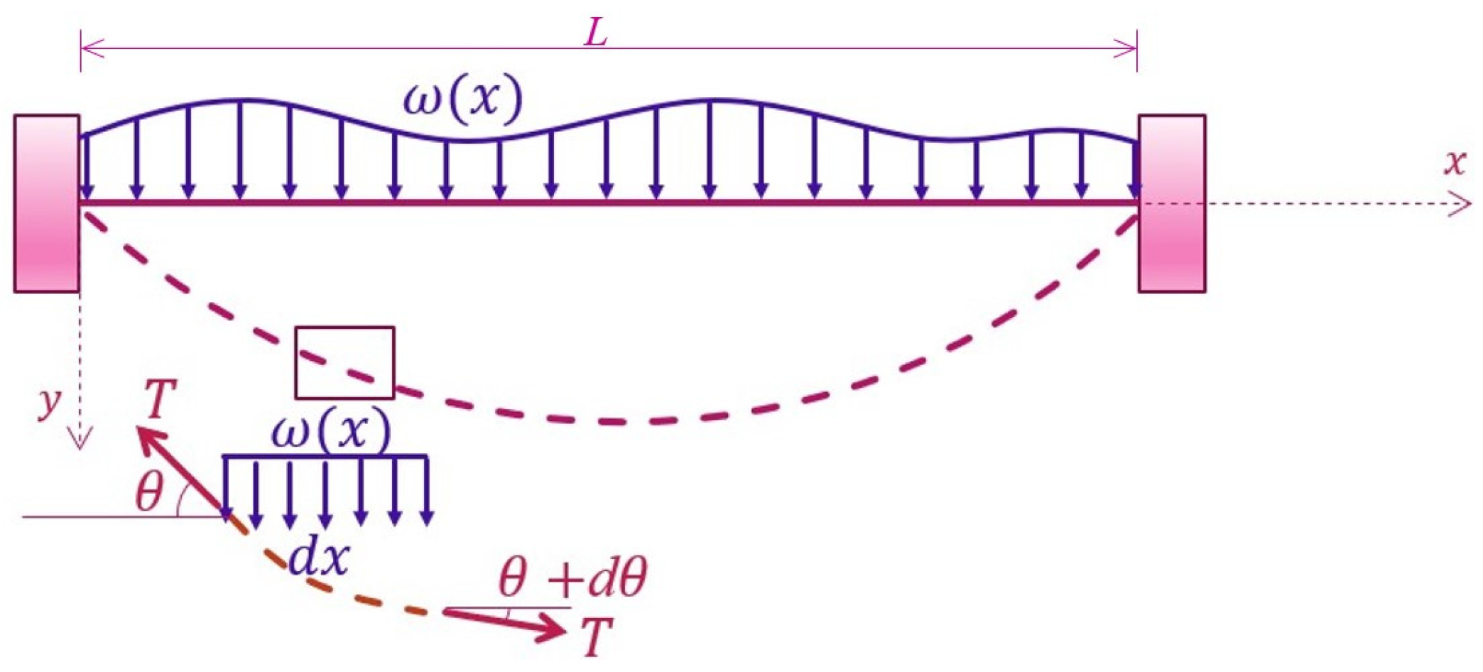
3.1. Tightly Stretched Wire under Loading

3.1.1. Problem Statement

Figure 1 shows the tightly stretched wire under distributed loading constrained at two ending points in which the total length of the wire is L and internal tension is T. We would like to predict the deflection of the tightly stretched wire under loading.
It is assumed that the internal tension is exceptionally large and the deflection of the tightly stretched wire is infinitesimal. The force balance equation is written as
T y,xx + ω = 0.
where the Dirichlet and Neumann boundary conditions are given as T y,x = h and y = g, respectively.

3.1.2. The Finite Element Model

Tightly stretched wires are evenly discretized into 100 elements with 101 nodes. For simplicity, we assume that the load only acts on the node. We randomly generated each nodal load within the range of 5 to 50 N. Three different cases, such as A, B, and C, are considered. Only one load is given on any random node in Case A. Totally, 101 loads are generated on all nodes in Case B. Loads from 1 to 101 are randomly generated on any node in Case C. To visualize node displacement during the simulation process, all node displacements are magnified to a certain extent, with a magnification of 100 times in Case B-C and 1000 times in Case A.

3.1.3. The Surrogate-Based PINN

Here, we use a single-layer neuron without a hidden layer as a surrogate of the FEM in which the values of nodal loading are the input data. It could be zero for the nodal point without load. We use cost function MSE and the Adam optimization scheme, where the batch is 10 in size. At last, the MSEs of all test sets are converged to be 0.01. It is indicated that solutions of the three cases are all accurate. At first, we use the same stiffness matrices in different cases, while we neglect biases. Thus, weight matrices in the neural network represent compliance matrices.
Next, we consider loading and tension as features. Then, we randomly set tensions ranging from 6000 to 10,000 N. That is, the stiffness of every sample is distinct. Here, the wire is assumed to be 10 m in length. To train the surrogate-based PINN, we randomly generate 10,000 samples for the FEM, where 16,000 samples are used for training and 4000 samples for testing.
Further, we construct two single-layer neurons, namely, NN1 and NN2. The input data of the first neuron consist of nodal loadings, and the output data consist of nodal displacements. The second neuron contains input internal tension T and nodal loadings, as well as output nodal deflections. Other hypotheses are identical to the previous one.
Having used length, loading, and tension as features, we randomly generate the wire in lengths ranging from 10 m to 100 m. We divide the wire to be 100 elements, where tension in the wire T is assumed from 6000 N to 10,000 N. Then, we conduct 10,000 finite element analyses.

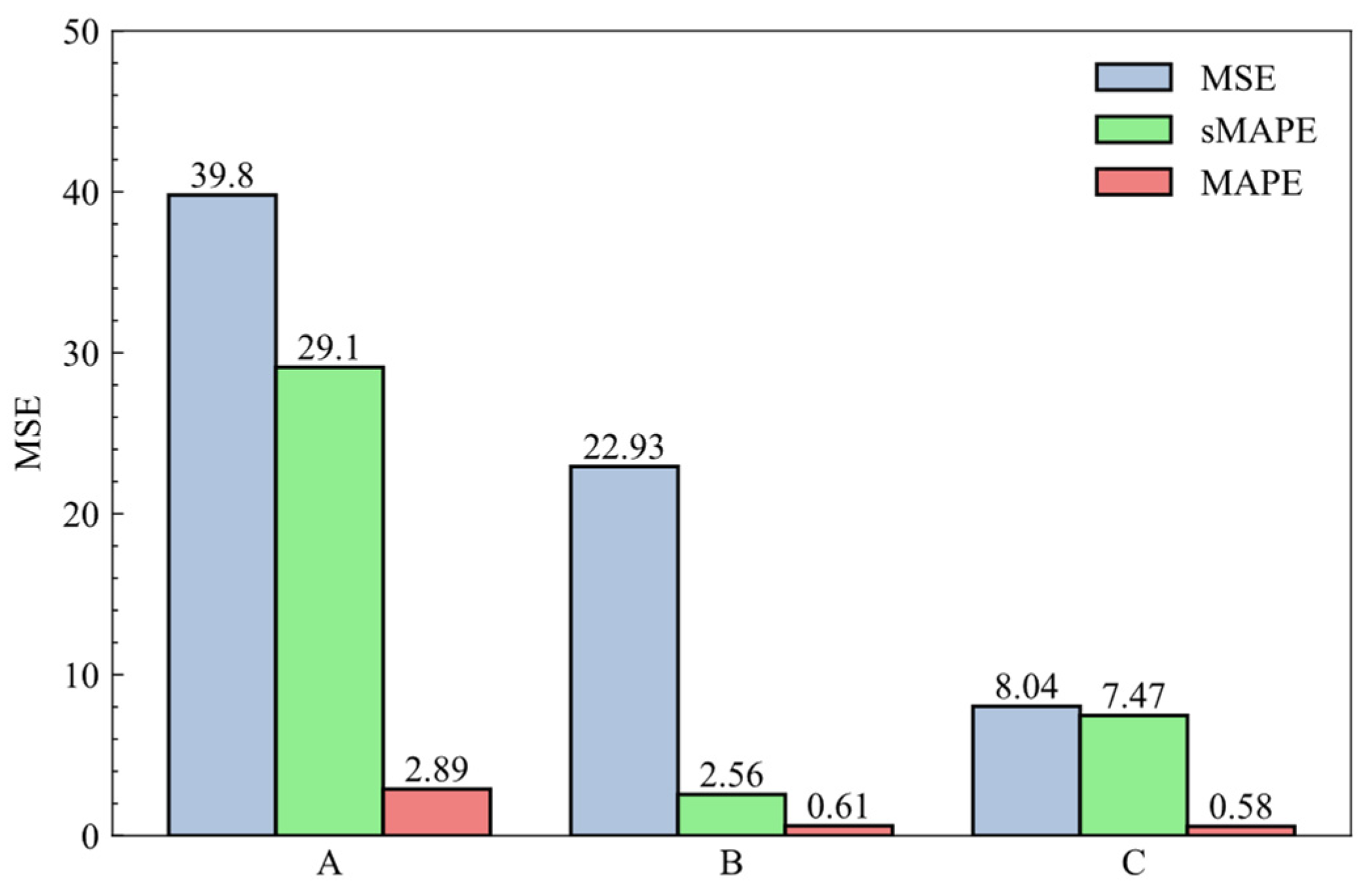
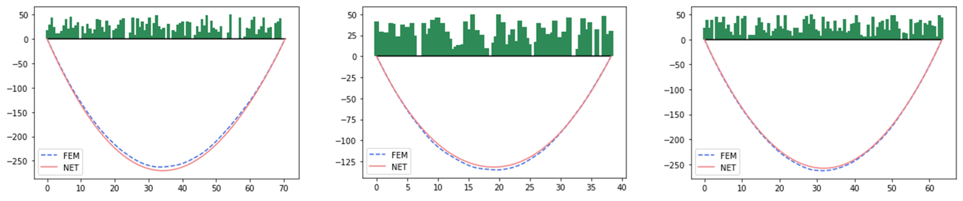
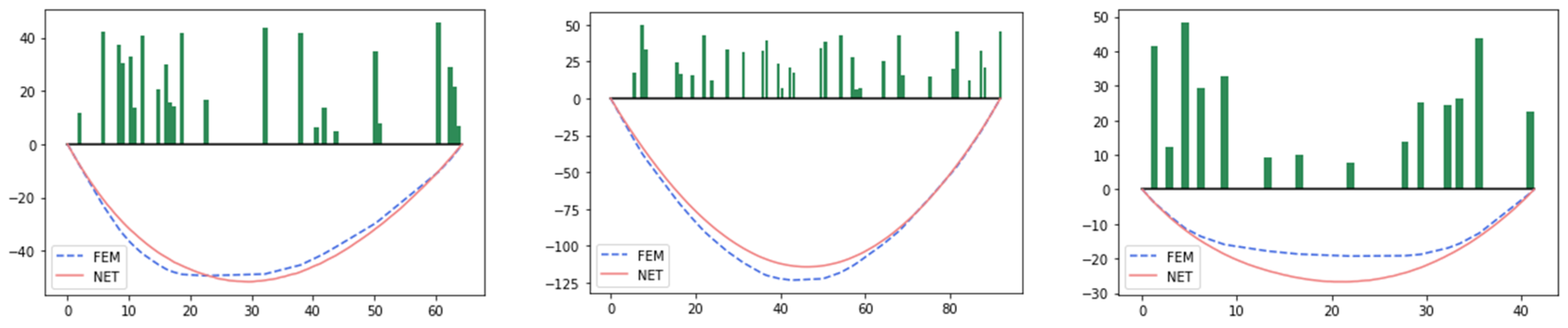
3.1.4. Results and Discussions

Figure 2 presents the MSE for three cases for different neural networks. That is, the results of NN2 are more accurate than those of NN1. For example, MSE is about 89% less than that of NN1 in Case B. When we take tension as an input vector, it is hard to obtain weights and biases utilizing shallow networks in cases with a linear stress–strain relation.
Thus, we generate the neural networks in which we consider coordinates, boundary conditions, nodal loadings, and tension as input data. NN3 is a convolution neural network with input data containing four channels. There are three convolution kernels in total. NN3 has 202 fully connected layers. The error in NN3 is the smallest when compared with the other two networks, and the MSE of NN3 is 0.58. We set the batch size as 128. The MSE is converged to about 22.8, and the SMAPE is converged to 6.9% after 250 epochs. Figure 3 illustrates several samples in the test set. The results of the neural networks are in good agreement with those of the FEM. Figure 4 reveals that the global error of some samples is small, but the deflection has a large oscillation, especially for those cases where loadings are sparse.

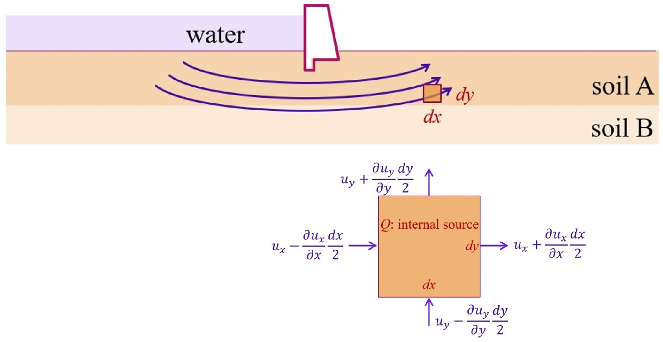
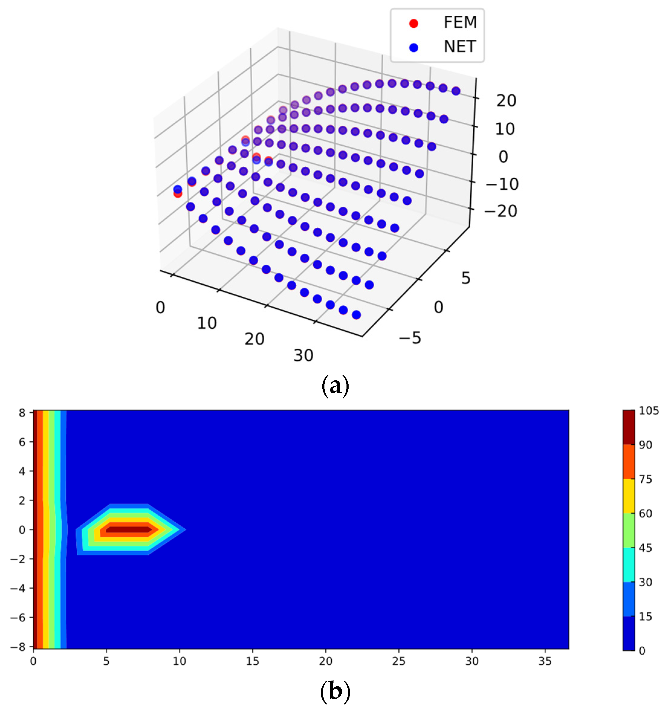
3.2. Flow through Porous Media

3.2.1. Problem Statement

As shown in Figure 5, a concrete gravity dam has a sheet pile in the upstream face to reduce the uplift pressure.
The total flow leaving through the surface must equal the internal sources Q. That is, ux,x + uy,y = Q, where ux and uy are the components of velocity at the centroid of the element. The Darcy formula declares that the average velocity in the pipe is proportional to the piezometric head. That is, ux = RxΦ,x and uy = RyΦ,y, where Rx and Ry are the coefficients of permeability; Φ is the piezometric head. Substitution into the previous equation yields
(RxΦ,x),x + (RyΦ,y),y = Q.
where Dirichlet and Neumann boundary conditions are given as RxΦ,xnx + RyΦ,yny = h and Φ = g, respectively.

3.2.2. The Finite Element Model

A concrete gravity dam has a sheet pile located at its upstream face to help reduce the uplift pressure under the dam. For the conditions shown, D denotes the depth of the sheet pile, B denotes the width, R denotes the permeability of soil, and Φ denotes the upstream head. We would like to determine the uplift pressure. Here, the depth of the sheet pile D is randomly generated from 5 to 20 m, the width B from 1 to 5 m, the permeability of soil R from 0 to 0.5 m/day, and the upstream head Φ from 5 to 30 m. For the configuration and mesh of the concrete gravity dam, please refer to the previous study [1].

3.2.3. The Surrogate-Based PINN

In the numerical example, we assume two boundary conditions. The first condition is impervious both upstream and downstream, and the second one is constant. To train the surrogate-based PINN, we randomly generate 10,000 samples for the FEM, where 16,000 samples are used for training and 4000 for testing.

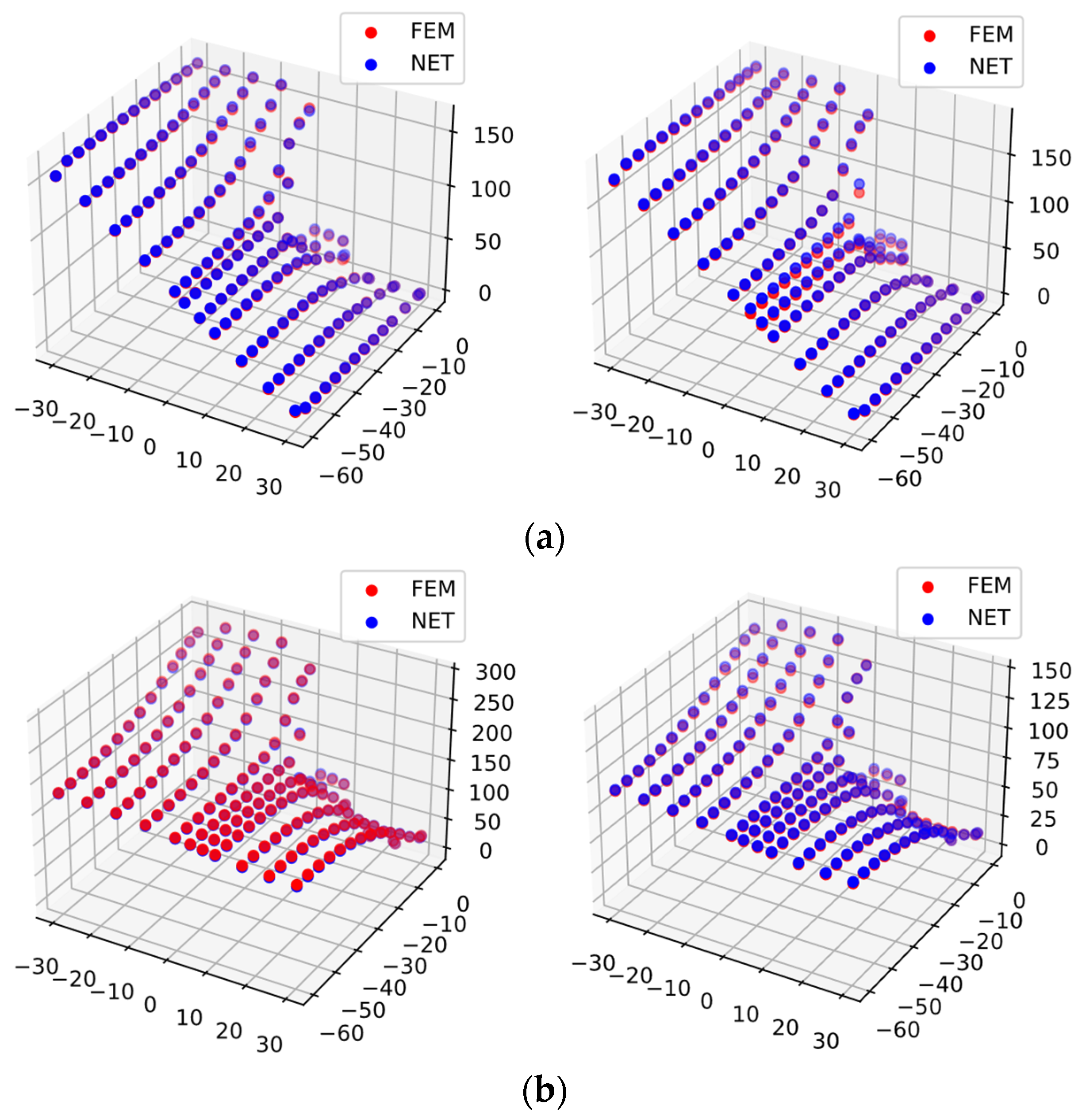
3.2.4. Results and Discussions

In this problem, the input layer has five channels, such as the x, y coordinates of nodal points, boundary constraints, hydrostatic heads on a boundary, and material properties. The input data are 5 × 154 × 1 in size. We use 5 convolution kernels and 308 fully connected layers. The output layer is 154 in length. We use MSE as the loss function and set the batch size as 128. Finally, the MSE of the test set is converged to about 7.9, and the SMAPE is set to approximately 7.1%. Figure 6 presents four representative samples in the test set. Predictions of the neural network are in good agreement with the approximated solutions using the FEM. It is demonstrated that the proposed deep learning technique is a good surrogate of the FEM.

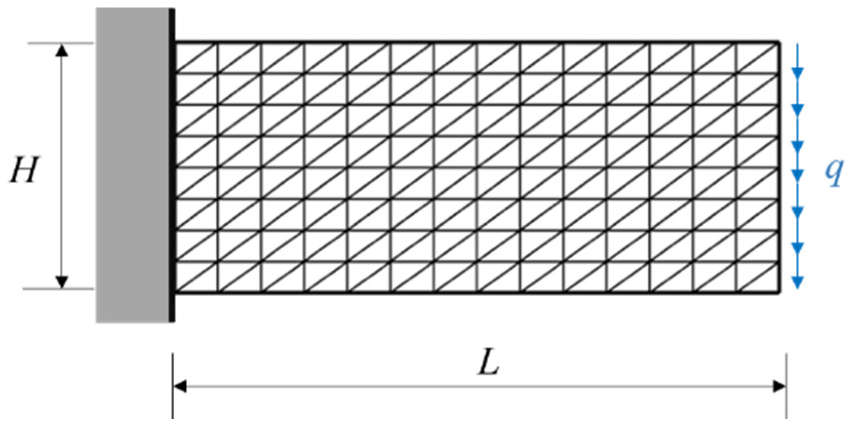
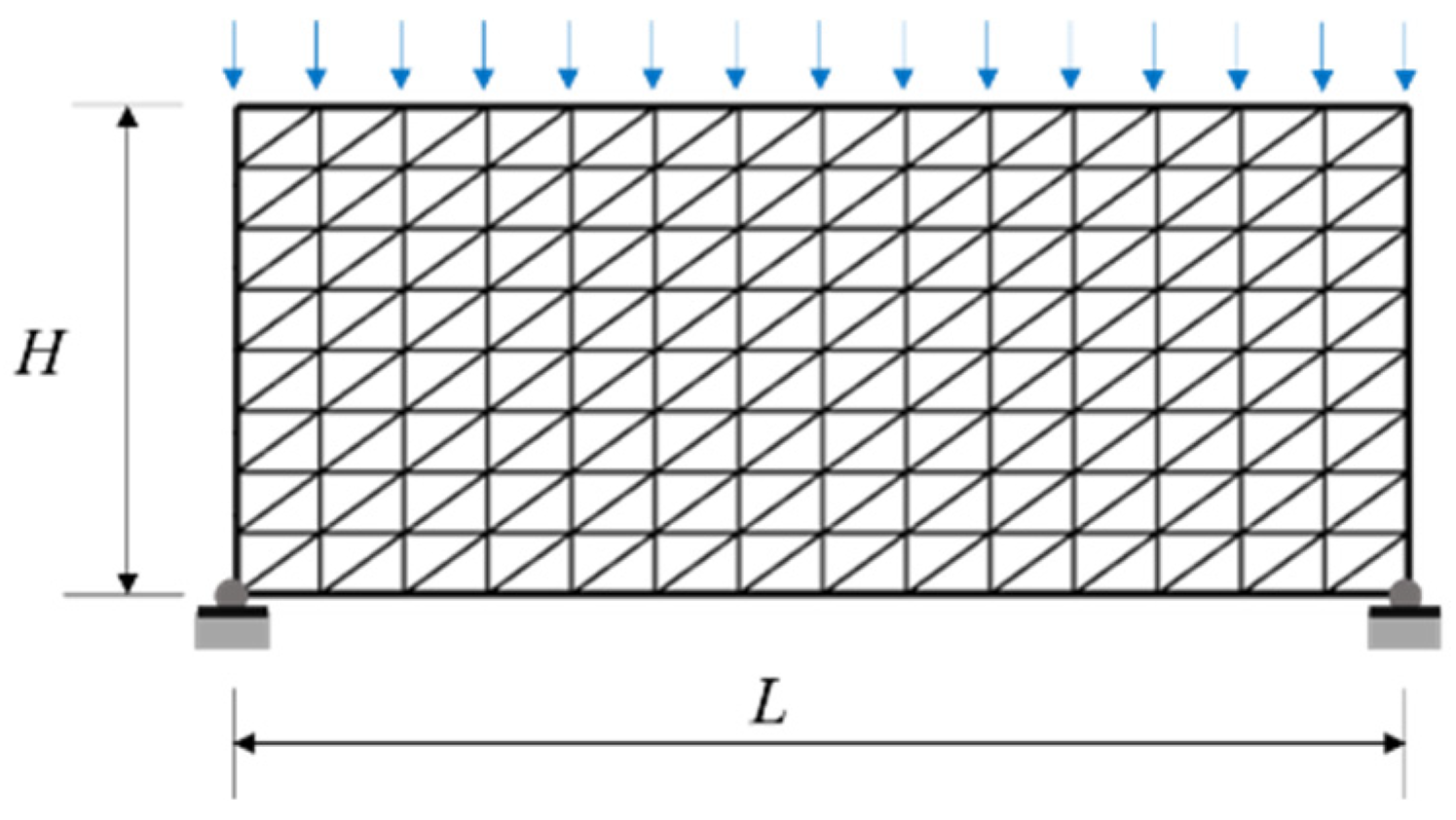
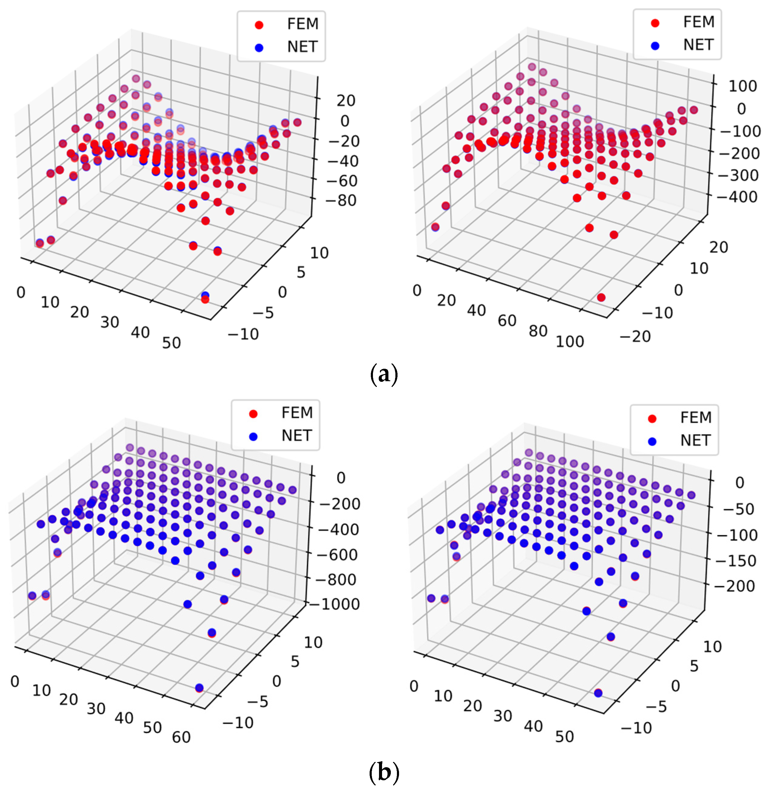
3.3. A Plane Cantilever Beam

3.3.1. Problem Statement

Figure 7 illustrates the plane cantilever beam under uniformly distributed loading at the end. Here, H denotes the height, L denotes the length, and q is the uniformly distributed loading at the end. We set the elastic modulus of the structure as E and the Poisson’s ratio as v. All governing equations are given in Equation (1).

3.3.2. The Finite Element Model

We discretize the domain of the beam into 224 three-node elements with 135 nodes to obtain the stress component σxx. Here, the height H is randomly generated from 10 to 50 m, the length L from 2 to 3 H, the uniformly distributed loading q from 0 to 100 N/m, the elastic modulus E from 1 × 10⁶ to 1 × 10⁷ Pa, and the Poisson ratio v from 0 to 0.5. To train the surrogate-based PINN, we randomly generate 10,000 samples for the FEM, where 16,000 samples are used for the training set and 4000 for testing.

3.3.3. The Surrogate-Based PINN

In this problem, the input layer has eight channels, such as the x, y coordinates of nodal points, boundary conditions at x, y directions, loadings at x, y directions, elastic modulus, and Poisson’s ratio. There are 8 convolution kernels and 270 units at the fully connected layer. We take the output of stress component σxx, use MSE as the loss function, and set the batch size to 256.

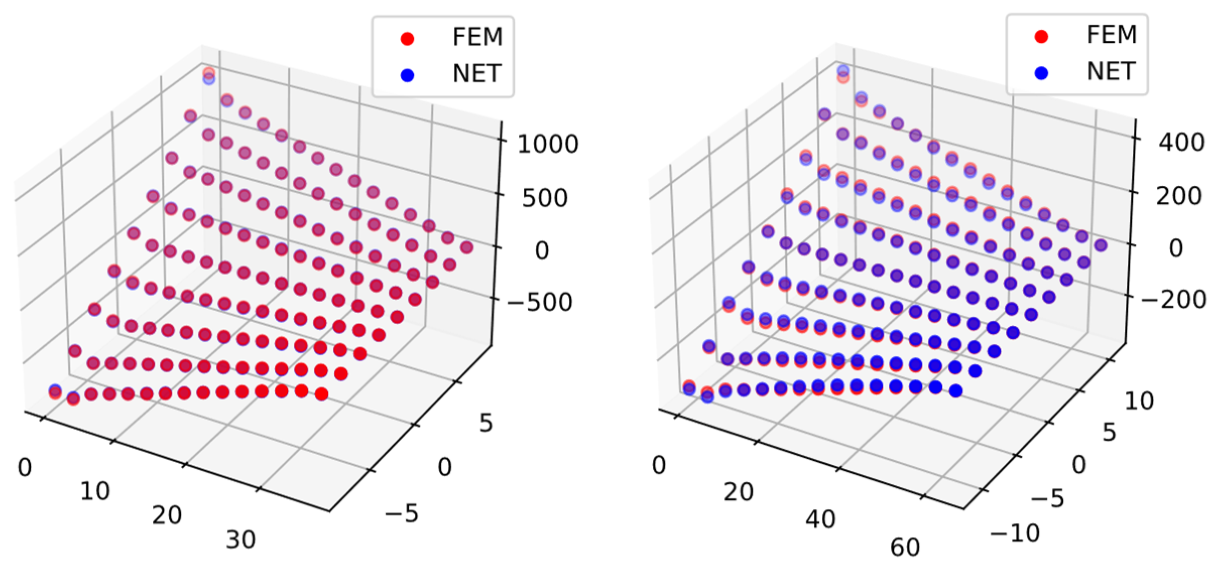
3.3.4. Results and Discussions

At last, the MSE of the test set is converged to approximately 75.62, the SMAPE is set to around 5.55%, and the MAPE is about 1.62%. Figure 8 shows the comparison between the results of the FEM and those of the neural network in which they are in good agreement. The proposed deep learning technique could be used to evaluate the contours of the stress field. Even though some oscillation appears somewhere, all errors are in an acceptable range.
The same neural network is used to predict the displacement in the x direction, ux. To better display the error, the displacement is expanded 10,000 times before training. After training, the MSE of the test set is converged to 9.01, the SMAPE is about 10.35%, and the MAPE is approximately 0.47%. Figure 9 shows the results of a typical case in the test set. The MSE in this case is converged to 4.16, the SMAPE is 9.27%, and the MAPE is 0.19%. It is seen from the SMAPE distribution that the errors are concentrated in the end boundary and the middle region. The displacement of these nodes is 0, so the SMAPE calculation produces large errors. There are nine nodes on the left end boundary, the FEM calculation result is about 1 × 10⁻¹², the neural network prediction result is about 1 × 10⁻³, and the SMAPE of nodes is about 100%. If the nine nodes are not considered for the error, the SMAPE is about 2.78%.

3.4. A Simply Supported Beam

3.4.1. Problem Statement

Figure 10 showed a simply supported beam in which the two ends on the bottom are fixedly connected, and the end on the top is subject to uniform pressure. The boundary and load conditions are changed just as the cantilever beam was in the previous section.

3.4.2. The Finite Element Model

The domain is divided into 224 elements and 135 nodes. In each sample, the values of length, width, elastic modulus, Poisson ratio, and load of the beam are assumed the same as the previous example. The size of the dataset and the structure of the neural network are the same as those in Section 3.3.1.

3.4.3. The Surrogate-Based PINN

At first, the neural network is trained separately to predict stress σxx and stress σyy. After training σxx, the error MSE of the test set is converged to 4.56, the SMAPE is 3.73%, and the MAPE is 0.80%. For σyy, the MSE of the test set is converged to 6.23, the SMAPE is 3.94%, and the MAPE is 0.42%. Figure 11 shows the prediction of stress using the finite element method and the neural network in the test set σxx and σyy.

3.4.4. Results and Discussions

The same neural network architecture is used to predict the displacement of the node in the y direction, uy, and the displacement is expanded 10,000 times before training. After training, the MSE of the test set is converged to 5.24, the SMAPE is 7.34%, and the MAPE is 10.30%. Figure 12 presents the comparison between the results of the FEM and those of the neural network.

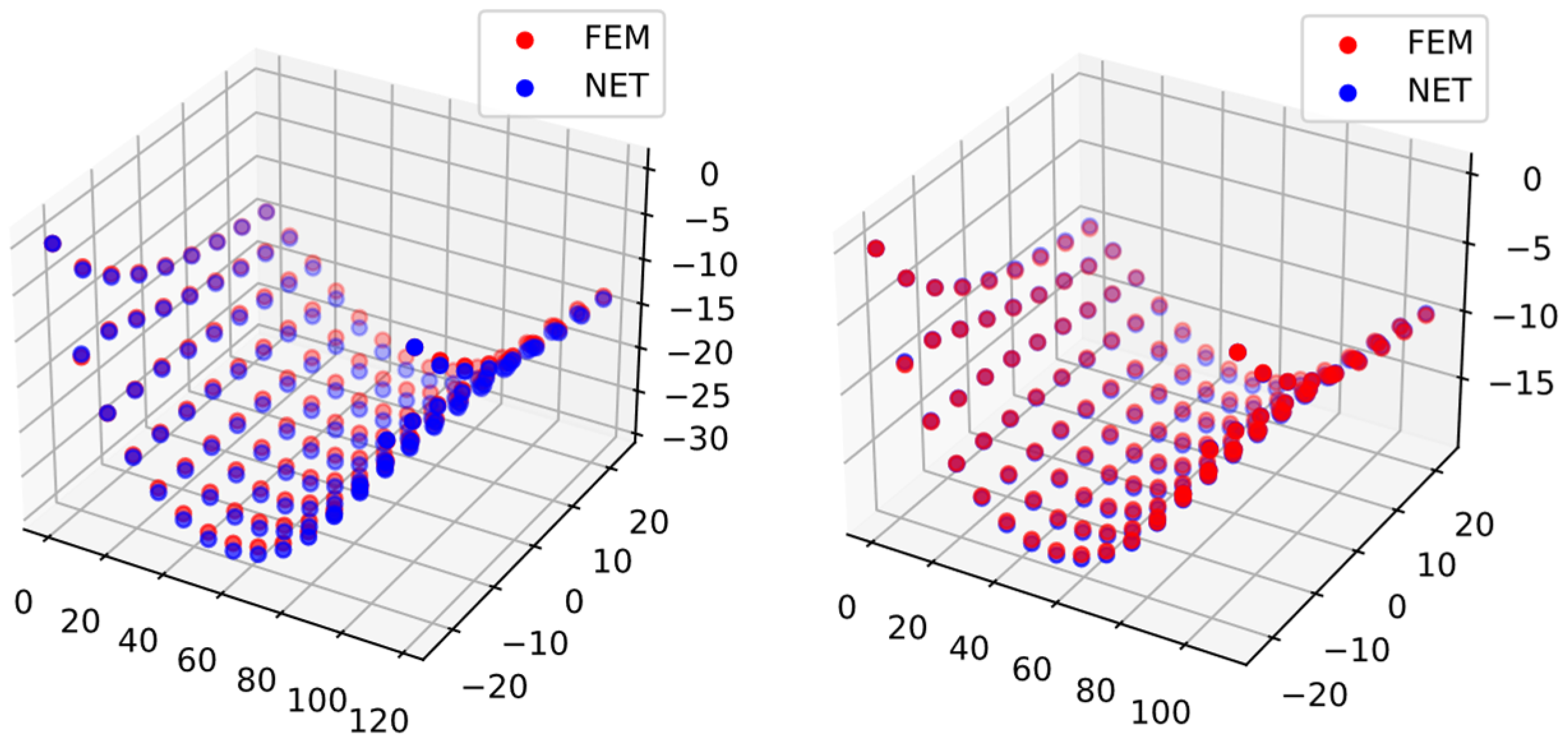
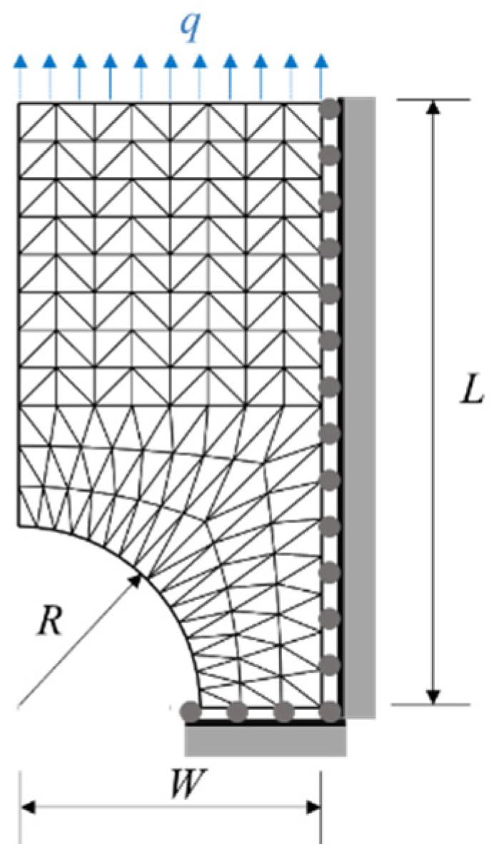
3.5. A Plate with Notch

3.5.1. Problem Statement

A plate is subjected to uniform tension at both ends, and there are semi-circular notches on both sides of the middle. Due to the symmetry of the plate, the solution domain only considers a quarter of the plate, shown in Figure 13, where L denotes the length of the part, W is the width, R is the radius of the notch, and q is the uniform tension at the end.

3.5.2. The Finite Element Model

We discretize the domain into 224 three-node elements with 140 nodes in the FEM model to determine the effective stress distribution σeff. Here, the radius of the notch R is randomly generated from 1 to 8 m, the width W from 10 to 20 m, the length L from 2 to 5 W, the uniform tension at the end q from 10 to 100 N/m, and the elastic modulus E from 1 × 10³ to 1×10⁴ Pa. To train the surrogate-based PINN, we randomly generate 10,000 samples for the FEM, where 16,000 samples are used for training and 4000 for testing.

3.5.3. The Surrogate-Based PINN

In this problem, the input layer has eight channels, such as the x, y coordinates of nodal points, boundary conditions at x, y directions, loadings at x, y directions, elastic modulus, and Poisson’s ratio. There are 8 convolution kernels and 280 units at the fully connected layer. We take the stress component σeff as the output, use MSE as the loss function, and set the batch size to 256.

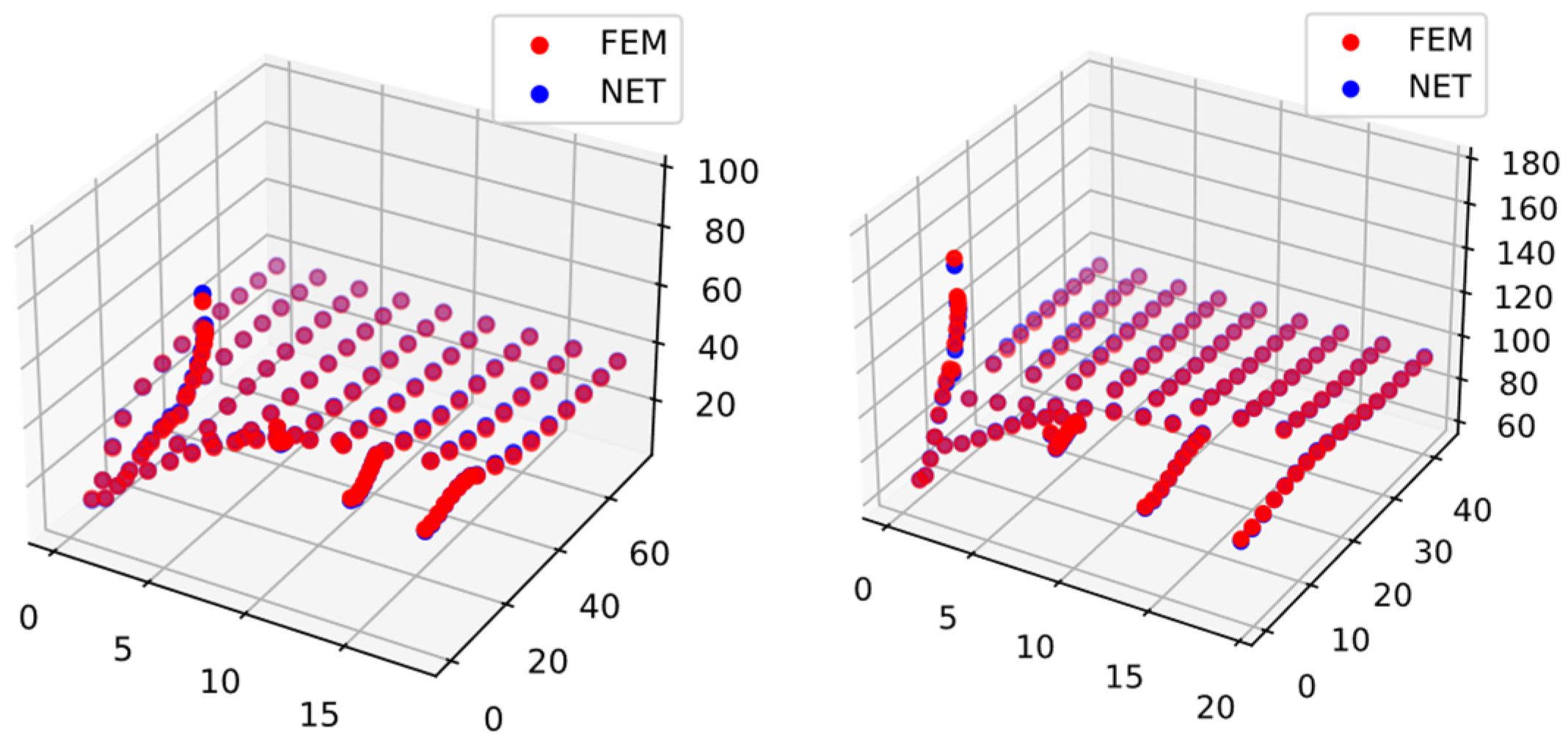
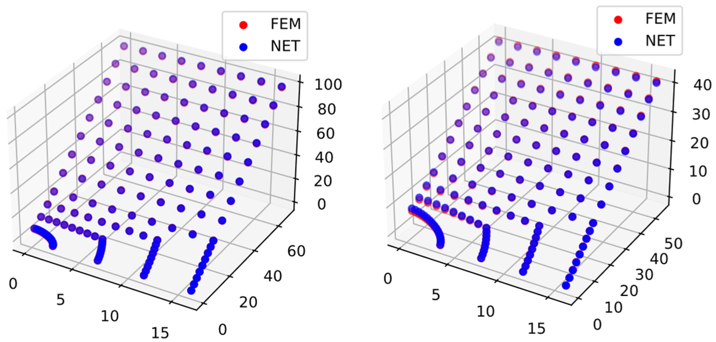
3.5.4. Results and Discussions

Finally, the MSE of the test set is converged to approximately 2.26, the SMAPE is set to around 1.21%, and the MAPE is set to about 0.89%. Figure 14 illustrates six examples randomly chosen from the test set. It is indicated that the proposed model could predict the stress field well, even around the notches.
The same neural network architecture is used to predict the displacement of a node in the y direction, uy, and the displacement is expanded 100 times before training. After many repetitions of training, the value is converged to 13.50 for MSE, 7.16% for SMAPE, and 3.02% for MAPE. Without considering the four bottom boundary nodes, the SMAPE is converged to 4.43%. Figure 15 shows the comparison between the FEM and neural network results.

4. Discussion

In general, there are three ways to improve the prediction accuracy of the neural network, such as adjusting the input variables, adjusting the structure of the neural network, and changing the loss function. Here, the influence of the loss function on error in neural networks is discussed based on data training. The loss function is set as the MSE in Equation (10) and the SMAPE in Equation (11). The cases of large displacement error predicted by the neural network are investigated.
Changing the original loss function from MSE to SMAPE or SMAPE combined with MSE could effectively reduce the error. It is indicated that using SMAPE as the loss function is more accurate for the prediction of non-zero values. However, it is found that SMAPE easily falls into the local optimal solution. Thus, the SMAPE is small, but the MSE is large. For this case, the errors of some nodes are larger than those of the surrounding nodes.
In addition, SMAPE and SMAPE combined with MSE are used as loss functions to predict displacements of the simply supported beam given in Section 3.3.2. In the case where SMAPE is used as the loss function, the network cannot obtain satisfactory results because the training of the neural network becomes stuck in the local optimal solution. When SMAPE combined with MSE is used as the loss function, the MSE of the test set is converged to 2.47, the SMAPE is 2.48%, and the MAPE is 1.49%.
In a word, it is indicated that while MSE is used as the loss function, the error is large, but the shape of contour is close to the true value. While SMAPE is used, it is easy to fall into the local optimal solution. Thus, SMAPE combined with MSE might be an excellent choice.
Finally, let us make a comparison of the time cost for the surrogate-based neural network technique and the conventional FEM. In Section 3.2, the average computation time of the finite element analyses for each numerical experiment is about 0.01888 s. However, it only takes 0.564 s to complete investigations of 1000 samples using the network. That is, the average computational time of the network is about 0.00056 s, about 33 times faster than that of the FEM. However, if the size of the training is set as 16,000, it would take an additional 302.112 s for the neural network to generate and train the model. In addition, the adjustment of the network architecture and parameter optimization are also time consuming.
In Section 3.3, the average computational time of the finite element analyses for each numerical experiment is about 0.0306 s. However, it only takes 0.583 s to analyze 1000 samples. That is, the average computational time of each sample is about 0.0306 s, around 52 times faster than that of the FEM. However, it would take an additional 244.576 s to generate and train 8000 specimens. In other words, generation and training are the price which the neural networks need to pay additionally.
In addition, the computational time of the neural network as a surrogate model depends on the building and debugging of the neural network. To reduce the errors of neural networks, it is necessary to select an appropriate neural network and to adjust the number of hidden layers and hidden units as well as the learning rate.
Furthermore, the computation of the FEM is related to the number of elements. For example, if the model in Section 3.3 is set to be 45 nodes and 64 three-node elements, the average computational time of each sample would be about 0.0129 s, saving 58% compared with 135-node cases. However, this is not an issue for the neural network.

5. Conclusions

In this paper, surrogate-based physics-informed neural networks (PINNs) were developed to solve representative boundary value problems based on elliptic partial differential equations (PDEs). Results from the proposed surrogate-based approach are in good agreement with those from the conventional FEM. For the tightly stretched wire problem, the SMAPE of the neural network was converged to approximately 6.9% for the test set. For the concrete gravity dam problem, the SMAPE of the test set was converged to about 7.1%. For the two-dimensional cantilever beam, the SMAPE of the test set to predict stress σxx was converged to around 4.3%, and the SMAPE of the test set to predict displacement ux was converged to about 9.9%. For the simply supported beam, the SMAPE of the test set to predict stress σyy was converged to approximately 3.9%, and the SMAPE of the test set to predict displacement uy was converged to around 9.9%. For the plate with notches, the SMAPE of the test set to predict stress σeff was converged to 1.2%, and the SMAPE of the test set to predict displacement uy was converged to 7.2%. It was indicated that trained neural networks could efficiently conduct numerical analysis for typical boundary value problems. That is, to some extent, the deep learning approach could replace the conventional numerical FEM as a great surrogate model.
In addition, it was found that modification of the loss function could improve the prediction accuracy of the neural network. Using the combination of SMAPE and MSE as the loss function could reduce errors, when compared with MSE as the loss function, and prevent it from falling into the local optimal solution during training. Furthermore, the prediction speed of the neural network is around 30–70 times faster than that of the FEM. Further, the surrogate-based PINN is independent on a number of elements and nodes. However, it takes time to generate, debug, and train the PINN model. It might be the price that artificial neural networks need to pay additionally. Even though PINN needs FEM results for training and is dependent on the FEM, we have started to explore and ponder what role artificial intelligence could play in computational mechanics.

Author Contributions

Conceptualization, Y.W.; methodology, P.Z.; software, C.Q.; validation, T.Z., X.W. and H.W.; formal analysis, P.Z.; investigation, C.Q.; resources, T.Z.; data curation, X.W.; writing—original draft preparation, P.Z.; writing—review and editing, Y.W.; visualization, H.W.; supervision, Y.W.; project administration, Y.W.; funding acquisition, Y.W. All authors have read and agreed to the published version of the manuscript.

Funding

This research is funded by the National Natural Science Foundation of China, grant number 52178299.

Data Availability Statement

The data presented in this study are available on request from the corresponding author. The data are not publicly available due to privacy.

Acknowledgments

The authors also want to thank Jesus Christ for listening to our prayers and the anonymous reviewers for their thorough review of the article and their constructive advice.

Conflicts of Interest

The authors declare no conflict of interest. The funders had no role in the design of this study; in the collection, analyses, or interpretation of data; in the writing of the manuscript; or in the decision to publish the results.

References

  1. Zhi, P.; Wu, Y. Finite element quantitative analysis and deep learning qualitative estimation in structural engineering. In Proceedings of the WCCM-XV, APCOM-VIII, Virtual Congress, 31 July 2022. [Google Scholar]
  2. Wu, Y.; Xiao, J. Implementation of the multiscale stochastic finite element method on elliptic PDE problems. Int. J. Comput. Methods 2017, 14, 1750003. [Google Scholar] [CrossRef]
  3. Wu, Y.; Xiao, J. The multiscale spectral stochastic finite element method for chloride diffusion in recycled aggregate concrete. Int. J. Comput. Methods 2018, 15, 1750078. [Google Scholar] [CrossRef]
  4. Wu, Y.; Xiao, J. Digital-image-driven stochastic homogenization for recycled aggregate concrete based on material microstructure. Int. J. Comput. Methods 2019, 16, 1850104. [Google Scholar] [CrossRef]
  5. Zhi, P.; Wu, Y. On the stress fluctuation in the smoothed finite element method for 2D elastoplastic problems. Int. J. Comput. Methods 2021, 18, 2150010. [Google Scholar] [CrossRef]
  6. Dissanayake, M.W.M.G.; Phan-Thien, N. Neural-network-based approximations for solving partial differential equations. Commun. Numer. Methods Eng. 1994, 10, 195–201. [Google Scholar] [CrossRef]
  7. Lagaris, I.E.; Likas, A.; Fotiadis, D.I. Artificial neural networks for solving ordinary and partial differential equations. IEEE Trans Neural. Netw. 1998, 9, 987–1000. [Google Scholar] [CrossRef] [PubMed] [Green Version]
  8. Poggio, T.; Mhaskar, H.; Rosasco, L. Why and when can deep-but not shallow-networks avoid the curse of dimensionality: A review. Int. J. Autom. Comput. 2017, 14, 503–519. [Google Scholar] [CrossRef] [Green Version]
  9. Raissi, M.; Perdikaris, P.; Karniadakis, G.E. Physics-informed neural networks: A deep learning framework for solving forward and inverse problems involving nonlinear partial differential equations. J. Comput. Phys. 2019, 378, 686–707. [Google Scholar] [CrossRef]
  10. Raissi, M. Deep hidden physics models: Deep learning of nonlinear partial differential equations. J. Mach Learn Res. 2018, 19, 1–24. [Google Scholar]
  11. Fang, Z.; Zhan, J. Deep physical informed neural networks for metamaterial design. IEEE Access 2019, 8, 24506–24513. [Google Scholar] [CrossRef]
  12. Raissi, M.; Yazdani, A.; Karniadakis, G.E. Hidden fluid mechanics: Learning velocity and pressure fields from flow visualizations. Science 2020, 367, 1026–1030. [Google Scholar] [CrossRef]
  13. Yang, L.; Meng, X.; Karniadakis, G.E. B-PINNs: Bayesian physics-informed neural networks for forward and inverse PDE problems with noisy data. J. Comput. Phys. 2021, 425, 109913. [Google Scholar] [CrossRef]
  14. Leung, W.T.; Lin, G.; Zhang, Z. NH-PINN: Neural homogenization-based physics-informed neural network for multiscale problems. J. Comput. Phys. 2022, 470, 111539. [Google Scholar] [CrossRef]
  15. Pang, G.; Lu, L.; Karniadakis, G.E. fPINNs: Fractional Physics-Informed Neural Networks. SIAM J. Sci. Comput. 2019, 41, A2603–A2626. [Google Scholar] [CrossRef] [Green Version]
  16. Pang, G.; D’Elia, M.; Parks, M.; Karniadakis, G.E. nPINNs: Nonlocal physics-informed neural networks for a parametrized nonlocal universal Laplacian operator. Algorithms and applications. J. Comput. Phys. 2020, 422, 109760. [Google Scholar] [CrossRef]
  17. Jagtap, A.D.; Karniadakis, G.E. Extended physics-informed neural networks (XPINNs): A Generalized Space-Time Domain Decomposition Based Deep Learning Framework for Nonlinear Partial Differential Equations. Commun. Comput. Phys. 2020, 28, 2002–2041. [Google Scholar]
  18. Haghighat, E.; Raissi, M.; Moure, A. A physics-informed deep learning framework for inversion and surrogate modeling in solid mechanics. Comput. Methods Appl. Mech. Eng. 2021, 379, 113741. [Google Scholar] [CrossRef]
  19. Lu, L.; Meng, X.; Mao, Z.; Karniadakis, G.E. DeepXDE: A deep learning library for solving differential equations. SIAM Rev. 2021, 63, 208–228. [Google Scholar] [CrossRef]
  20. Sirignano, J.; Spiliopoulos, K. DGM: A deep learning algorithm for solving partial differential equations. J. Comput. Phys. 2018, 375, 1339–1364. [Google Scholar] [CrossRef] [Green Version]
  21. Samaniego, E.; Anitescu, C.; Goswami, S. An energy approach to the solution of partial differential equations in computational mechanics via machine learning: Concepts, implementation and applications. Comput. Methods Appl. Mech. Eng. 2020, 362, 112790. [Google Scholar] [CrossRef] [Green Version]
  22. Liang, L.; Liu, M.; Martin, C.; Sun, W. A deep learning approach to estimate stress distribution: A fast and accurate surrogate of finite-element analysis. J. R. Soc. Interface 2018, 15, 20170844. [Google Scholar] [CrossRef] [Green Version]
  23. Nourbakhsh, M.; Irizarry, J.; Haymaker, J. Generalizable surrogate model features to approximate stress in 3D trusses. Eng. Appl. Artif. Intell. 2018, 71, 15–27. [Google Scholar] [CrossRef]
  24. Abueidda, D.W.; Almasri, M.; Ammourah, R. Prediction and optimization of mechanical properties of composites using convolutional neural networks. Compos Struct. 2019, 227, 111264. [Google Scholar] [CrossRef] [Green Version]
  25. Nie, Z.; Jiang, H.; Kara, L.B. Stress field prediction in cantilevered structures using convolutional neural networks. J. Comput. Inf. Sci. Eng. 2020, 20, 1–8. [Google Scholar] [CrossRef] [Green Version]
  26. Jiang, H.; Nie, Z.; Yeo, R. StressGAN: A generative deep learning model for two-dimensional stress distribution prediction. J. Appl. Mech 2021, 88, 1–9. [Google Scholar] [CrossRef]
  27. Lin, S.; Zheng, H.; Han, C. Evaluation and prediction of slope stability using machine learning approaches. Front. Struct. Civ. Eng. 2021, 15, 821–833. [Google Scholar] [CrossRef]
  28. Tabarsa, A.; Latifi, N.; Osouli, A.; Bagheri, Y. Unconfined compressive strength prediction of soils stabilized using artificial neural networks and support vector machines. Front. Struct. Civ. Eng. 2021, 15, 520–536. [Google Scholar] [CrossRef]
  29. Le, H.Q.; Truong, T.T.; Dinh-Cong, D.; Nguyen-Thoi, T. A deep feed-forward neural network for damage detection in functionally graded carbon nanotube-reinforced composite plates using modal kinetic energy. Front. Struct. Civ. Eng. 2021, 15, 1453–1479. [Google Scholar] [CrossRef]
  30. Savino, P.; Tondolo, F. Automated classification of civil structure defects based on convolutional neural network. Front. Struct. Civ. Eng. 2021, 15, 305–317. [Google Scholar] [CrossRef]
  31. Bekdaş, G.; Yücel, M.; Nigdeli, S.M. Estimation of optimum design of structural systems via machine learning. Front. Struct. Civ. Eng. 2021, 15, 1441–1452. [Google Scholar] [CrossRef]
  32. Carbas, S.; Artar, M. Comparative seismic design optimization of spatial steel dome structures through three recent metaheuristic algorithms. Front. Struct. Civ. Eng. 2022, 16, 57–74. [Google Scholar] [CrossRef]
  33. Kellouche, Y.; Ghrici, M.; Boukhatem, B. Service life prediction of fly ash concrete using an artificial neural network. Front. Struct. Civ. Eng. 2021, 15, 793–805. [Google Scholar] [CrossRef]
  34. Teng, S.; Chen, G.; Wang, S. Digital image correlation-based structural state detection through deep learning. Front. Struct. Civ. Eng. 2022, 16, 45–56. [Google Scholar] [CrossRef]
  35. LeCun, Y.; Bengio, Y.; Hinton, G. Deep learning. Nature 2015, 521, 436–444. [Google Scholar] [CrossRef]
  36. Krizhevsky, A.; Sutskever, I.; Hinton, G.E. ImageNet classification with deep convolutional neural networks. Commun. ACM 2017, 60, 84–90. [Google Scholar] [CrossRef] [Green Version]
Figure 1. The tightly stretched wire under distributed loading.
Mathematics 11 02723 g001
Figure 2. MSE of three cases for different neural networks.
Mathematics 11 02723 g002
Figure 3. The three samples in the test set where the green bars represent the magnitude and location of loading.
Mathematics 11 02723 g003
Figure 4. Notable samples in the test set where the green bars represent the magnitude and location of loading.
Mathematics 11 02723 g004
Figure 5. A concrete gravity dam.
Mathematics 11 02723 g005
Figure 6. Samples randomly chosen in the test set: (a) constant heads, and (b) impervious boundaries.
Mathematics 11 02723 g006
Figure 7. The plane cantilever beam under uniformly distributed loading at the end.
Mathematics 11 02723 g007
Figure 8. Comparison between results of the FEM and those of the neural network.
Mathematics 11 02723 g008
Figure 9. A sample in the test set with the SMAPE as 9.27% and the MAPE as 0.19%: (a) solutions from the FEM and those of the neural network and the (b) SMAPE distribution.
Mathematics 11 02723 g009
Figure 10. The simply supported beam is subjected to a uniform load from the top.
Mathematics 11 02723 g010
Figure 11. Comparison between the FEM and NET for several samples in the test set of (a) σxx and (b) σyy.
Mathematics 11 02723 g011
Figure 12. Comparison between results of the FEM and those of the neural network.
Mathematics 11 02723 g012
Figure 13. Configuration and mesh of the plate with notches.
Mathematics 11 02723 g013
Figure 14. Comparison between σeff values of the FEM and those of the neural network.
Mathematics 11 02723 g014
Figure 15. Comparison between uy values of the FEM and those of the neural network.
Mathematics 11 02723 g015
Disclaimer/Publisher’s Note: The statements, opinions and data contained in all publications are solely those of the individual author(s) and contributor(s) and not of MDPI and/or the editor(s). MDPI and/or the editor(s) disclaim responsibility for any injury to people or property resulting from any ideas, methods, instructions or products referred to in the content.

