Exponential Stability of a Class of Neutral Inertial Neural Networks with Multi-Proportional Delays and Leakage Delays

Abstract

This paper investigates the exponential stability of a class of neutral inertial neural networks with multi-proportional delays and leakage delays. By utilizing the Lyapunov stability theory, the approach of parametric variation, and the differential inequality technique, some criteria are acquired that can guarantee that all solutions of the addressed system converge exponentially to the equilibrium point. In particular, the neutral term, multi-proportional delays, and leakage delays are incorporated simultaneously, resulting in a more general model, and the findings are novel and refine the previous works. Finally, one example is provided to indicate that the dynamic behavior is consistent with the theoretical analysis.

1. Introduction

In recent years, more and more scholars have endeavored to provide in-depth analyses of neural networks (NNs) in terms of their applications in different kinds of areas, including pattern recognition, combinatorial optimization, associative memory, automatic control, and so on [1,2,3]. These applications greatly hinge on the dynamic characteristic of NNs. Unlike ordinary NNs, inertial terms were initially incorporated into NNs by Babcock and Westervelt [4] in 1987, which were called inertial neural networks (INNs). As a second-order dynamic system, INNs have rich dynamic characteristics [5,6] involving periodic solutions, quasi-periodic solutions, bifurcation, and chaos phenomena. In the real world, inertia terms play an important role in the disordered search of memory. Meanwhile, INNs could also be viewed as one class of mathematical models in fields such as biological systems and mechanical projects [7].

Additionally, time delays ubiquitously exist in networks, which usually result in harmful effects on systems, including oscillation, bifurcation, or chaos. In general, time delays are composed of bounded delays and unbounded delays. Many results have been reported on the dynamic behavior analysis of INNs with bounded delays, and two main approaches, i.e., variable transformation and the non-reduced order method, were developed in [8,9,10,11]. Meanwhile, proportional delay (PD) can be considered as a special kind of unbounded delays, and in reality, it also plays a key role in, for example, the collection of current by the pantograph of an electric locomotive and the web quality of routing decisions. Meanwhile, leakage delay, as one typical delay, also appears in neural network models and leads to the destabilization of the networks. Currently, various dynamic behaviors of INNs with proportional delays (PDs) or leakage delays have been deeply investigated. In [12,13,14], stability issue of INNs with PDs were examined by choosing a suitable Lyapunov functional and utilizing inequality techniques. In [15], the periodicity of inertial Cohen–Grossberg NNs with PDs has been analyzed according to the differential inclusions and coincidence theorem. In [16], dissipativity of fuzzy cellular INNs with PDs has been considered in virtue of the linear matrix inequality (LMI) technique. In [17], the synchronization of two nonidentical complex-valued INNs with leakage delays was explored, and the sliding-mode control laws have been designed.

Neutral-type delays were first introduced by Hale and Lunel [18] in physical and chemical processes, and aeroelasticity, which reflected that current states of systems depended on the variation rate of the past states. Subsequently, they have been gradually applied to population systems, circuits systems, automatic control, and neural networks. Neutral NNs could be seen as one special class of time-delay network systems [19,20]. Recently, dynamic characteristics and control issues of neutral inertial neural networks (NINNs) have received extensive attention. In [21,22], the asymptotical stability and Lagrange stability of NINNs have been investigated using the LMI technique and the Lyapunov method. In [23,24], the dissipativity of memristor-based NINNs has been analyzed, and the issue of fixed-time stabilization for a class of fuzzy NINNs has been tackled by means of one novel fixed-time stability theory in [25]. It can be seen that the above results [21,22,23,24,25,26] consider the bounded neutral delays, and the unbounded cases such as neutral proportional delays are not discussed. Furthermore, quite a few publications about stability analysis of neutral recurrent NNs with PDs have sprung up. For instance, in [27], the global exponential convergence for one kind of high-order cellular NNs with neutral PDs has been examined by employing the Lyapunov function approach and the differential inequality technique. Furthermore, theoretical results [27] have been extended to neutral-type Hopfield NNs with PDs and leakage delays in [28]. For neutral cellular NNs with PDs and a D-operator, global exponential stability has been investigated in virtue of the mathematical proof by contradiction in [29,30,31]. In [32], the asymptotic stability issue of quaternion-valued neutral NNs with leakage delay and PDs has been handled by employing the principle of homeomorphism, the LMI technique, and Lyapunov stability theory. For NINNs with PDs and time-variable coefficients, finite time synchronization has been investigated using finite time stability theory in [33]. It is worth noting that in [33], proportional delays and external inputs have no influence on the results, essentially since the controllers are introduced and the activation functions are required to be bounded. Furthermore, if these limited conditions are removed, it must be determined how to deal with the problem of exponential stability of NINNs with PDs and leakage delays. Up to now, there is still hardly any reference considering this issue. Therefore, this paper aims to fill this gap.

Inspired by the above discussions, we study the global exponential stability for a class of NINNs with multi-proportional delays and leakage delays using the Lyapunov function method and the differential inequality technique. The main contributions are summarized in terms of three aspects. Firstly, INNs introduced in this paper are more general and complicated since the inertial term, variable coefficients, external inputs and various delays, including neutral delays, PDs, and leakage delays, are considered simultaneously. Secondly, due to the existence of different kinds of delays, one new differential inequality technique combined with the Lyapunov function method is developed. Unlike the existing results, the proportional delays have an important impact on the system, and the activation functions are not required to be bounded. Thirdly, several sufficient conditions are acquired to ensure the exponential stability of NINNs with PDs and leakage delays, and the exponential convergence rate also is estimated. The remainder of this paper is arranged as follows. In Section 2, several standard notations and complicated models are introduced, and some fundamental assumptions are imposed. In Section 3, based on the Lyapunov stability theory and differential inequality techniques, some novel criteria for exponential stability for the addressed system are established. In Section 4, one example and numerical simulations are provided to show the effectiveness of the previous proposed findings. One brief conclusion is finally drawn.

Notations. 

In our article, the following standard notations are adopted. Let $\mathbb{R}$ and ${\mathbb{R}}^{+}$ denote the set of real numbers and the set of non-negative real numbers, respectively. ${\mathbb{R}}^n$ denotes the set of all n-dimensional real column vectors. For any $z={(z_1,z_2,\cdots ,z_n)}^T\in {\mathbb{R}}^n$, $z^T$ represents the transposition of vector z. $\left|z\right|$ is defined by $\left|z\right|={(\left|z_1\right|,\left|z_2\right|,\cdots ,\left|z_n\right|)}^T$ and $∥z∥={\max }_{i\in \mathbb{I}}\left|z_i\right|$, where $∥·∥$ stands for the vector norm and $\mathbb{I}=\{1,2,\cdots ,n\}$. $C_{}^1([\sigma t_0,t_0];\mathbb{R})$ represents the continuous and first-order differentiable function family from $[\sigma t_0,t_0],(t_0>0,0<\sigma <1)$ to $\mathbb{R}$. For an arbitrary given bounded function F, we define $F^{+}={sup}_{t\in \left[t_0,+\infty \right)}\left|F\left(t\right)\right|$, $F^{-}={inf}_{t\in \left[t_0,+\infty \right)}\left|F\left(t\right)\right|$.

2. Preliminaries

Consider one class of NINNs with multi-proportional delays and leakage delays as shown below:

$$\begin{array}{c}\left\{\begin{array}{cc}\hfill v_i^{″}\left(t\right)=& -a_i\left(t\right)v_i^{\prime }\left(t\right)-b_i\left(t\right)v_i(t-{\lambda }_i\left(t\right))+\sum _{j=1}^n{d}_{ij}\left(t\right){\tilde{f}}_j\left(v_j\left(t\right)\right)+\sum _{j=1}^n{c}_{ij}\left(t\right){\tilde{g}}_j\left(v_j\left({\rho }_{ij}t\right)\right)\hfill \\ \hfill & +\sum _{j=1}^n{l}_{ij}\left(t\right){\tilde{h}}_j\left(v_j^{\prime }\left({\gamma }_{ij}t\right)\right)+J_i\left(t\right),t\ge t_0>0,\hfill \\ \\ v_i\left(z\right)=\hfill & {\phi }_i\left(z\right),v_i^{\prime }\left(z\right)={\phi }_i^{\prime }\left(z\right),z\in [\sigma t_0,t_0],i=1,2,\cdots ,n.\hfill \end{array}\right.\hfill \end{array}$$

(1)

where $v_i\left(t\right)$ denotes the ith neuron state at time t, and the second derivative $v_i^{″}\left(t\right)$ is called an inertial term of Equation (1). $a_i\left(t\right),b_i\left(t\right)$ are two bounded functions; $d_{ij}\left(t\right),c_{ij}\left(t\right)$, and $l_{ij}\left(t\right)$ represent the connection weights associated with neurons without delays and with delays at time t. ${\lambda }_i\left(t\right)$ is called leakage delay. Moreover, we assume that functions $d_{ij}\left(t\right),c_{ij}\left(t\right),l_{ij}\left(t\right),J_i\left(t\right)\in \left[t_0,+\infty \right)⟶\mathbb{R}$ and ${\lambda }_i\left(t\right):\left[t_0,+\infty \right)⟶{\mathbb{R}}^{+}$ are piecewise continuous and bounded. ${\rho }_{ij},{\gamma }_{ij}$ represent proportional delay factors, which satisfy $0<{\rho }_{ij}<1,0<{\gamma }_{ij}<1$. Obviously, proportional delays ${\rho }_{ij}t,{\gamma }_{ij}t$ can be rewritten by ${\rho }_{ij}t=t-(1-{\rho }_{ij})t,{\gamma }_{ij}t=t-(1-{\gamma }_{ij})t$. It can be seen that $(1-{\rho }_{ij})t⟶+\infty ,(1-{\gamma }_{ij})t⟶+\infty$ as $t⟶+\infty$. ${\tilde{f}}_j,{\tilde{g}}_j,{\tilde{h}}_j:\mathbb{R}⟶\mathbb{R}$ denote neuron activation functions with ${\tilde{f}}_j\left(0\right)={\tilde{g}}_j\left(0\right)={\tilde{h}}_j\left(0\right)=0$. $J_i\left(t\right)$ denotes the external input. Let the initial value ${\phi }_i\left(z\right)$ satisfy ${\phi }_i\left(z\right)\in C^1([\sigma t_0,t_0];\mathbb{R})$, $\sigma ={min}_{i,j\in \mathbb{J}}\{{\rho }_{ij},{\gamma }_{ij}\}$.

For system (1), we utilize the variable transformation

$$\begin{array}{c}\begin{array}{c}{u}_i\left(t\right)=v_i^{\prime }\left(t\right)+{\delta }_i{v}_i\left(t\right),i\in \mathbb{I},\hfill \end{array}\hfill \end{array}$$

(2)

where ${\delta }_i$ denotes one chosen positive parameter. Let $p_i\left(t\right)=a_i\left(t\right)-{\delta }_i,k_i\left(t\right)=-b_i\left(t\right)+{\delta }_i{p}_i\left(t\right)$. Accordingly, NINNs (1) is rewritten by the equation

$$\begin{array}{c}\left\{\begin{array}{cc}{v}_i^{\prime }\left(t\right)=\hfill & -{\delta }_i{v}_i\left(t\right)+u_i\left(t\right),\hfill \\ u_i^{\prime }\left(t\right)=\hfill & -p_i\left(t\right)u_i\left(t\right)+k_i\left(t\right)v_i\left(t\right)+b_i\left(t\right)v_i\left(t\right)-b_i\left(t\right)v_i(t-{\lambda }_i\left(t\right))\hfill \\ \hfill & +\sum _{j=1}^n{d}_{ij}\left(t\right){\tilde{f}}_j\left(v_j\left(t\right)\right)+\sum _{j=1}^n{c}_{ij}\left(t\right){\tilde{g}}_j\left(v_j\left({\rho }_{ij}t\right)\right)+\sum _{j=1}^n{l}_{ij}\left(t\right){\tilde{h}}_j\left(v_j^{\prime }\left({\gamma }_{ij}t\right)\right)+J_i\left(t\right),\hfill \\ v_i\left(z\right)=\hfill & {\phi }_i\left(z\right),u_i\left(z\right)=v_i^{\prime }\left(z\right)+{\delta }_i{v}_i\left(z\right)={\psi }_i\left(z\right),z\in [\sigma t_0,t_0],t_0>0,i\in \mathbb{I}.\hfill \end{array}\right.\hfill \end{array}$$

(3)

Furthermore, we impose the following assumptions on system (1), which are quite necessary in acquiring our new findings.

($H_1$) For each $i\in \mathbb{I}$, suppose that there exists a bounded and continuous function ${\overline{p}}_i:\left[t_0,+\infty \right)\to (0,+\infty )$ and a positive constant $M_i$ satisfying

$$\begin{array}{c}{e}^{-{\int }_z^t{p}_i\left(\theta \right)d\theta }\le M_i{e}^{-{\int }_z^t{\overline{p}}_i\left(\theta \right)d\theta }\forall t,z\in [t_0,+\infty ).\hfill \end{array}$$

(4)

($H_2$) For $\forall w\in \mathbb{R}$, $j\in \mathbb{I}$, suppose that there are non-negative constants $L_j^{\tilde{f}}$, $L_j^{\tilde{g}}$, $L_j^{\tilde{h}}$ satisfying

$$\begin{array}{c}|{\tilde{f}}_j\left(w\right)|\le L_j^{\tilde{f}}\left|w\right|,|{\tilde{g}}_j\left(w\right)|\le L_j^{\tilde{g}}\left|w\right|,|{\tilde{h}}_j\left(w\right)|\le L_j^{\tilde{h}}\left|w\right|.\hfill \end{array}$$

(5)

($H_3$) Suppose that there exist several positive constants ${\xi }_1,{\xi }_2,\dots ,{\xi }_n,{\eta }_1,{\eta }_2,\dots ,{\eta }_n$, and ${\beta }_0$ such that

$$\begin{array}{c}-{\delta }_i+\frac{{\eta }_i}{{\xi }_i}<0,{\delta }_i+\frac{{\eta }_i}{{\xi }_i}<1,\underset{t\ge t_0}{sup}\left\{-{\overline{p}}_i\left(t\right)+M_i{G}_i\left(t\right)\right\}<0,i\in \mathbb{I},\hfill \end{array}$$

(6)

and

$$\begin{array}{c}{J}_i\left(t\right)=O\left(e^{-{\beta }_{0}t}\right)\mathrm{as}t\to +\infty ,\hfill \end{array}$$

(7)

where

$$\begin{array}{c}\begin{array}{cc}{G}_i\left(t\right)=\hfill & {\eta }_i^{-1}{\xi }_i|k_i\left(t\right)|+{\eta }_i^{-1}|b_i\left(t\right)|{\lambda }_i^{+}{e}^{{\beta }_0{\lambda }_i^{+}}+{\eta }_i^{-1}\sum _{j=1}^n|d_{ij}\left(t\right)|L_j^{\tilde{f}}{\xi }_j\hfill \\ \hfill & +{\eta }_i^{-1}\sum _{j=1}^n|c_{ij}\left(t\right)|L_j^{\tilde{g}}{\xi }_j{e}^{{\beta }_0(1-{\rho }_{ij})t}+{\eta }_i^{-1}\sum _{j=1}^n\left|l_{ij}\left(t\right)\right|L_j^{\tilde{h}}{\xi }_j{e}^{{\beta }_0(1-{\gamma }_{ij})t}.\hfill \end{array}\hfill \end{array}$$

(8)

3. Main Results

In this section, by means of the differential inequality technique and the Lyapunov function approach, the global exponential stability of a class of NINNs with proportional delays and leakage delays is examined.

Theorem 1.

Suppose that assumptions $\left(H_1\right)$–$\left(H_3\right)$ hold. Then, for any solution to Equation (3), there is one constant $\beta \in \left(0,{\beta }_0\right)$ satisfying

$$\begin{array}{c}{v}_i\left(t\right)=O\left(e^{-\beta t}\right),v_i^{\prime }\left(t\right)=O\left(e^{-\beta t}\right),u_i\left(t\right)=O\left(e^{-\beta t}\right)\mathrm{as}t\to +\infty ,i\in \mathbb{I}.\hfill \end{array}$$

(9)

Proof. 

Let $z\left(t\right)={\left(v_1\left(t\right),v_2\left(t\right),\dots ,v_n\left(t\right),u_1\left(t\right),u_2\left(t\right),\dots ,u_n\left(t\right)\right)}^T$ denote a solution to Equation (3) for the given initial value $v_i\left(z\right)={\phi }_i\left(z\right),u_i\left(z\right)={\psi }_i\left(z\right),z\in [\sigma t_0,t_0]$. Resorting to the following variable transformation

$$\begin{array}{c}\left\{\begin{array}{cc}x\left(t\right)=\hfill & {(x_1\left(t\right),x_2\left(t\right),\dots ,x_n\left(t\right))}^T={({\xi }_1^{-1}{v}_1\left(t\right),{\xi }_2^{-1}{v}_2\left(t\right),\dots ,{\xi }_n^{-1}{v}_n\left(t\right))}^T,\hfill \\ y\left(t\right)=\hfill & {(y_1\left(t\right),y_2\left(t\right),\dots ,y_n\left(t\right))}^T={({\eta }_1^{-1}{u}_1\left(t\right),{\eta }_2^{-1}{u}_2\left(t\right),\dots ,{\eta }_n^{-1}{u}_n\left(t\right))}^T,\hfill \end{array}\right.\hfill \end{array}$$

(10)

Equation (3) is transformed into the following equation:

$$\begin{array}{c}\left\{\begin{array}{cc}{x}_i^{\prime }\left(t\right)=\hfill & -{\delta }_i{x}_i\left(t\right)+{\xi }_i^{-1}{\eta }_i{y}_i\left(t\right),\hfill \\ y_i^{\prime }\left(t\right)=\hfill & -p_i\left(t\right)y_i\left(t\right)+{\eta }_i^{-1}{k}_i\left(t\right)v_i\left(t\right)+{\eta }_i^{-1}{b}_i\left(t\right)v_i\left(t\right)-{\eta }_i^{-1}{b}_i\left(t\right)v_i(t-{\lambda }_i\left(t\right))\hfill \\ \hfill & +{\eta }_i^{-1}\sum _{j=1}^n{d}_{ij}\left(t\right){\tilde{f}}_j\left(v_j\left(t\right)\right)+{\eta }_i^{-1}\sum _{j=1}^n{c}_{ij}\left(t\right){\tilde{g}}_j\left(v_j\left({\rho }_{ij}t\right)\right)\hfill \\ \hfill & +{\eta }_i^{-1}\sum _{j=1}^n{l}_{ij}\left(t\right){\tilde{h}}_j\left(v_j^{\prime }\left({\gamma }_{ij}t\right)\right)+{\eta }_i^{-1}{J}_i\left(t\right),\hfill \end{array}\right.\hfill \end{array}$$

(11)

According to assumption $\left(H_3\right)$, we may select one parameter $\beta \in (0,min\{{\beta }_0,{min}_{i\in \mathbb{I}}\{{\xi }_i,$${inf}_{t\ge t_0}{\overline{p}}_i\left(t\right)\left\}\right\})$ such that

$$\begin{array}{c}\begin{array}{c}\beta -{\delta }_i+\frac{{\eta }_i}{{\xi }_i}<0,\underset{t\ge t_0}{sup}\left\{\beta -{\overline{p}}_i\left(t\right)+M_i\left[G_i\left(t\right)+\beta \right]\right\}<0,i\in \mathbb{I}.\hfill \end{array}\hfill \end{array}$$

(12)

Moreover, we have that

$$\begin{array}{c}\begin{array}{cc}sup\hfill & \{\beta -{\overline{p}}_i\left(t\right)+M_i[{\eta }_i^{-1}{\xi }_i|v_i\left(t\right)|+{\eta }_i^{-1}\sum _{j=1}^n\left|d_{ij}\left(t\right)\right|L_j^{\tilde{f}}{\xi }_j\hfill \\ \hfill & +{\eta }_i^{-1}\sum _{j=1}^n|c_{ij}\left(t\right)|L_j^{\tilde{g}}{\xi }_j{e}^{\beta (1-{\rho }_{ij})t}+{\eta }_i^{-1}\sum _{j=1}^n\left|l_{ij}\left(t\right)\right|L_j^{\tilde{h}}{\xi }_j{e}^{\beta (1-{\gamma }_{ij})t}+\beta \left]\right\}\hfill \\ \hfill & \le \underset{t\ge t_0}{sup}\{\beta -{\overline{p}}_i\left(t\right)+M_i[G_i\left(t\right)+\beta ]\}<0,i\in \mathbb{I}.\hfill \end{array}\hfill \end{array}$$

(13)

Let $\parallel \mathsf{\Phi }\parallel =max\{{max}_{i\in \mathbb{I}}\{{\xi }_i^{-1}{max}_{t\in [\sigma t_0,t_0]}|{\phi }_i\left(t\right)\left|\right\},{max}_{i\in \mathbb{I}}\{{\eta }_i^{-1}{max}_{t\in [\sigma t_0,t_0]}|{\psi }_i\left(t\right)\left|\right\},{max}_{i\in \mathbb{I}}\{{\xi }_i^{-1}{max}_{t\in [\sigma t_0,t_0]}|{\phi }_i^{\prime }\left(t\right)\left|\right\}\}$. For $\forall \zeta >0$ and $\forall K\ge 1$, obviously, we can acquire the result that

$$\begin{array}{c}\begin{array}{c}max\left\{\right|x_i\left(t\right)|,|y_i\left(t\right)|,|x_i^{\prime }\left(t\right)\left|\right\}\le K(\parallel \mathsf{\Phi }\parallel +\zeta )e^{-\beta (t-t_0)},\forall t\in [\sigma t_0,t_0]\hfill \end{array}\hfill \end{array}$$

(14)

Furthermore, by assumption $\left(H_3\right)$, we may find a large enough parameter $K>{max}_{i\in \mathbb{I}}{M}_i+1\ge 1$ such that

$$\begin{array}{c}\begin{array}{c}|{\eta }_i^{-1}{J}_i\left(t\right)|<\beta K(\parallel \mathsf{\Phi }\parallel +\zeta )e^{-\beta (t-t_0)},\forall t\ge t_0>0,i\in \mathbb{I}.\hfill \end{array}\hfill \end{array}$$

(15)

Subsequently, we need to claim that

$$\begin{array}{c}\begin{array}{c}max\left\{|x_i\left(t\right)|,|y_i\left(t\right)|,|x_i^{\prime }\left(t\right)|\right\}<K(\parallel \mathsf{\Phi }\parallel +\zeta )e^{-\beta (t-t_0)},\forall t>t_0.\hfill \end{array}\hfill \end{array}$$

(16)

Assume that Equation (16) does not hold; then, there must exist $i\in \mathbb{I}$ and $\tilde{t}>t_0$ satisfying

$$\begin{array}{c}\begin{array}{c}max\left\{\right|x_i\left(\tilde{t}\right)|,|y_i\left(\tilde{t}\right)|,|x_i^{\prime }\left(\tilde{t}\right)\left|\right\}=K(\parallel \mathsf{\Phi }\parallel +\zeta )e^{-\beta (\tilde{t}-t_0)},\hfill \end{array}\hfill \end{array}$$

(17)

and

$$\begin{array}{c}\begin{array}{c}max\left\{\right|x_i\left(t\right)|,|y_i\left(t\right)|,|x_i^{\prime }\left(t\right)\left|\right\}<K(\parallel \mathsf{\Phi }\parallel +\zeta )e^{-\beta (t-t_0)},\forall t\in [\sigma t_0,\tilde{t}).\hfill \end{array}\hfill \end{array}$$

(18)

Noting that $x_i^{\prime }\left(t\right)=-{\delta }_i{x}_i\left(t\right)+{\xi }_i^{-1}{\eta }_i{y}_i\left(t\right)$, its solution could be denoted by

$$\begin{array}{c}\begin{array}{c}{x}_i\left(t\right)=x_i\left(t_0\right)e^{-{\delta }_i\left(t-t_0\right)}+{\int }_{t_0}^t{e}^{-{\delta }_i(t-z)}{\xi }_i^{-1}{\eta }_i{y}_i\left(z\right)dz,z\in \left[t_0,t\right],t\in \left[t_0,\tilde{t}\right).\hfill \end{array}\hfill \end{array}$$

(19)

Therefore, we can obtain the result that

$$\begin{array}{c}\begin{array}{cc}\left|x_i\left(\tilde{t}\right)\right|\hfill & =\left|x_i\left(t_0\right)e^{-{\delta }_i\left(\tilde{t}-t_0\right)}+{\int }_{t_0}^{\tilde{t}}{e}^{-{\delta }_i(\tilde{t}-z)}{\xi }_i^{-1}{\eta }_i{y}_i\left(z\right)dz\right|\hfill \\ \hfill & \le \left|x_i\left(t_0\right)\right|e^{-{\delta }_i\left(\tilde{t}-t_0\right)}+{\int }_{t_0}^{\tilde{t}}{e}^{-{\delta }_i(\tilde{t}-z)}{\xi }_i^{-1}{\eta }_i\left|y_i\left(z\right)\right|dz\hfill \\ \hfill & \le |x_i\left(t_0\right)|e^{-{\delta }_i(\tilde{t}-t_0)}+{\int }_{t_0}^{\tilde{t}}{e}^{-{\delta }_i(\tilde{t}-z)}{\xi }_i^{-1}{\eta }_{i}K(\parallel \mathsf{\Phi }\parallel +\zeta )e^{-\beta (z-t_0)}dz\hfill \\ \hfill & <(\parallel \mathsf{\Phi }\parallel +\zeta )e^{-\beta (\tilde{t}-t_0)}{e}^{-({\delta }_i-\beta )(\tilde{t}-t_0)}+{\int }_{t_0}^{\tilde{t}}{e}^{-({\delta }_i-\beta )(\tilde{t}-z)}{\xi }_i^{-1}{\eta }_{i}dzK(\parallel \mathsf{\Phi }\parallel +\zeta )e^{-\beta (\tilde{t}-t_0)}\hfill \\ \hfill & <\left(\parallel \mathsf{\Phi }\parallel +\zeta \right)e^{-\beta \left(\tilde{t}-t_0\right)}\left[e^{-\left({\delta }_i-\beta \right)\left(\tilde{t}-t_0\right)}+K{\int }_{t_0}^{\tilde{t}}{e}^{-\left({\delta }_i-\beta \right)(\tilde{t}-z)}\left({\delta }_i-\beta \right)dz\right]\hfill \\ \hfill & <K\left(\parallel \mathsf{\Phi }\parallel +\zeta \right)e^{-\beta \left(\tilde{t}-t_0\right)}\left[e^{-\left({\delta }_i-\beta \right)\left(\tilde{t}-t_0\right)}\left(\frac{1}{K}-1\right)+1\right]\hfill \\ \hfill & <K\left(\parallel \mathsf{\Phi }\parallel +\zeta \right)e^{-\beta \left(\tilde{t}-t_0\right)}.\hfill \end{array}\hfill \end{array}$$

(20)

Combining assumption $\left(H_3\right)$ and Equation (17), we also acquire that

$$\begin{array}{c}\begin{array}{cc}|x_i^{\prime }\left(\tilde{t}\right)|\hfill & =|-{\delta }_i{x}_i\left(\tilde{t}\right)+{\xi }_i^{-1}{\eta }_i{y}_i\left(\tilde{t}\right)|\hfill \\ \hfill & \le ({\delta }_i+{\xi }_i^{-1}{\eta }_i)max\left\{\right|x_i\left(\tilde{t}\right)|,|y_i\left(\tilde{t}\right)|,|x_i^{\prime }\left(\tilde{t}\right)\left|\right\}\hfill \\ \hfill & =({\delta }_i+{\xi }_i^{-1}{\eta }_i)K(\parallel \mathsf{\Phi }\parallel +\zeta )e^{-\beta (\tilde{t}-t_0)}\hfill \\ \hfill & <K(\parallel \mathsf{\Phi }\parallel +\zeta )e^{-\beta (\tilde{t}-t_0)}.\hfill \end{array}\hfill \end{array}$$

(21)

According to Equation (11), it is noted that

$$\begin{array}{c}\begin{array}{cc}{y}_i^{\prime }\left(z\right)+p_i\left(z\right)y_i\left(z\right)=\hfill & {\eta }_i^{-1}{k}_i\left(z\right)v_i\left(z\right)+{\eta }_i^{-1}{b}_i\left(z\right){\int }_{z-{\lambda }_i\left(z\right)}^z{v}_i^{\prime }\left(\theta \right)d\theta +{\eta }_i^{-1}\sum _{j=1}^n{d}_{ij}\left(z\right){\tilde{f}}_j\left(v_j\left(z\right)\right)\hfill \\ \hfill & +{\eta }_i^{-1}\sum _{j=1}^n{c}_{ij}\left(z\right){\tilde{g}}_j\left(v_j\left({\rho }_{ij}z\right)\right)+{\eta }_i^{-1}\sum _{j=1}^n{l}_{ij}\left(z\right){\tilde{h}}_j\left(v_j^{\prime }\left({\gamma }_{ij}z\right)\right)\hfill \\ \hfill & +{\eta }_i^{-1}{J}_i\left(z\right),z\in \left[t_0,t\right],t\in \left[t_0,\tilde{t}\right).\hfill \end{array}\hfill \end{array}$$

(22)

Moreover, we may find that the solution satisfies that

$$\begin{array}{c}\begin{array}{cc}{y}_i\left(t\right)=\hfill & y_i\left(t_0\right)e^{-{\int }_{t_0}^t{p}_i\left(\theta \right)d\theta }+{\int }_{t_0}^t{e}^{-{\int }_z^t{p}_i\left(\theta \right)d\theta }[{\eta }_i^{-1}{k}_i\left(z\right)v_i\left(z\right)+{\eta }_i^{-1}{b}_i\left(z\right){\int }_{z-{\lambda }_i\left(z\right)}^z{v}_i^{\prime }\left(\theta \right)d\theta \hfill \\ \hfill & +{\eta }_i^{-1}\sum _{j=1}^n{d}_{ij}\left(z\right){\tilde{f}}_j\left(v_j\left(z\right)\right)+{\eta }_i^{-1}\sum _{j=1}^n{c}_{ij}\left(z\right){\tilde{g}}_j\left(v_j\left({\rho }_{ij}z\right)\right)\hfill \\ \hfill & +{\eta }_i^{-1}\sum _{j=1}^n{l}_{ij}\left(z\right){\tilde{h}}_j\left(v_j^{\prime }\left({\gamma }_{ij}z\right)\right)+{\eta }_i^{-1}{J}_i\left(z\right)]dz.\hfill \end{array}\hfill \end{array}$$

(23)

Together with Equations (13), (15) and (18), by computing, one has the result that

$$\begin{array}{c}\begin{array}{cc}|y_i\left(\tilde{t}\right)|=\hfill & |y_i\left(t_0\right)e^{-{\int }_{t_0}^{\tilde{t}}{p}_i\left(\theta \right)d\theta }+{\int }_{t_0}^{\tilde{t}}{e}^{-{\int }_z^{\tilde{t}}{p}_i\left(\theta \right)d\theta }[{\eta }_i^{-1}{k}_i\left(z\right)v_i\left(z\right)+{\eta }_i^{-1}{b}_i\left(z\right){\int }_{z-{\lambda }_i\left(z\right)}^z{v}_i^{\prime }\left(\theta \right)d\theta \hfill \\ \hfill & +{\eta }_i^{-1}\sum _{j=1}^n{d}_{ij}\left(z\right){\tilde{f}}_j\left(v_j\left(z\right)\right)+{\eta }_i{}^{-1}\sum _{j=1}^n{c}_{ij}\left(z\right){\tilde{g}}_j\left(v_j\left({\rho }_{ij}z\right)\right)\hfill \\ \hfill & +{\eta }_i^{-1}\sum _{j=1}^n{l}_{ij}\left(z\right){\tilde{h}}_j\left(v_j^{\prime }\left({\gamma }_{ij}z\right)\right)+{\eta }_i^{-1}{J}_i\left(z\right)\left]dz\right|\hfill \\ \hfill \le & |y_i(t_0|M_i{e}^{-{\int }_{t_0}^{\tilde{t}}{\overline{p}}_i\left(\theta \right)d\theta }+{\int }_{t_0}^{\tilde{t}}{e}^{-{\int }_z^{\tilde{t}}{\overline{p}}_i\left(\theta \right)d\theta }{M}_i[{\eta }_i^{-1}{\xi }_i|k_i\left(z\right)||x_i\left(z\right)|\hfill \\ \hfill & +{\eta }_i^{-1}|b_i\left(z\right)||{\lambda }_i\left(z\right)||v_i^{\prime }(z-{\lambda }_i\left(z\right)|+{\eta }_i^{-1}\sum _{j=1}^n|d_{ij}\left(z\right)|L_j^{\tilde{f}}{\xi }_j|x_i\left(z\right)|\hfill \\ \hfill & +{\eta }_i^{-1}\sum _{j=1}^n|c_{ij}\left(z\right)|L_j^{\tilde{g}}{\xi }_j|x_j\left({\rho }_{ij}z\right)|+{\eta }_i^{-1}\sum _{j=1}^n|l_{ij}\left(z\right)|L_j^{\tilde{h}}{\xi }_j|x_j^{\prime }\left({\gamma }_{ij}z\right)|+{\eta }_i^{-1}{J}_i\left(z\right)]dz\hfill \\ \hfill <& (\parallel \mathsf{\Phi }\parallel +\zeta )M_i{e}^{-{\int }_{t_0}^{\tilde{t}}{\overline{p}}_i\left(\theta \right)d\theta }+{\int }_{t_0}^{\tilde{t}}{e}^{-{\int }_z^{\tilde{t}}{\overline{p}}_i\left(\theta \right)d\theta }{M}_i[{\eta }_i^{-1}{\xi }_i|k_i\left(z\right)|K(\parallel \mathsf{\Phi }\parallel +\zeta )e^{-\beta (z-t_0)}\hfill \\ \hfill & +{\eta }_i^{-1}|b_i\left(z\right)|{\lambda }_i\left(z\right)K(\parallel \mathsf{\Phi }\parallel +\zeta )e^{-\beta (z-{\lambda }_i\left(z\right)-t_0)}\hfill \\ \hfill & +{\eta }_i^{-1}\sum _{j=1}^n|d_{ij}\left(z\right)|L_j^{\tilde{f}}{\xi }_{j}K(\parallel \mathsf{\Phi }\parallel +\zeta )e^{-\beta (z-t_0)}\hfill \\ \hfill & +{\eta }_i^{-1}\sum _{j=1}^n|c_{ij}\left(z\right)|L_j^{\tilde{g}}{\xi }_{j}K(\parallel \mathsf{\Phi }\parallel +\zeta )e^{-\beta ({\rho }_{ij}z-t_0)}\hfill \\ \hfill & +{\eta }_i^{-1}\sum _{j=1}^n|l_{ij}\left(z\right)|L_j^{\tilde{h}}{\xi }_{j}K(\parallel \mathsf{\Phi }\parallel +\zeta )e^{-\beta ({\gamma }_{ij}z-t_0)}+\beta K(\parallel \mathsf{\Phi }\parallel +\zeta )e^{-\beta (z-t_0)}]dz\hfill \\ \hfill <& (\parallel \mathsf{\Phi }\parallel +\zeta )M_i{e}^{-{\int }_{t_0}^{\tilde{t}}{\overline{p}}_i\left(\theta \right)d\theta }+{\int }_{t_0}^{\tilde{t}}{e}^{-{\int }_z^{\tilde{t}}({\overline{p}}_i\left(\theta \right)-\beta )d\theta }{M}_i[{\eta }_i^{-1}{\xi }_i|k_i\left(z\right)|+{\eta }_i^{-1}|b_i\left(z\right)|{\lambda }_i^{+}{e}^{\beta {\lambda }_i^{+}}+\hfill \\ \hfill & {\eta }_i^{-1}\sum _{j=1}^n|d_{ij}\left(z\right)|L_j^{\tilde{f}}{\xi }_j+{\eta }_i^{-1}\sum _{j=1}^n|c_{ij}\left(z\right)|L_j^{\tilde{g}}{\xi }_j{e}^{\beta (1-{\rho }_{ij})z}+{\eta }_i^{-1}\sum _{j=1}^n|l_{ij}\left(z\right)|L_j^{\tilde{h}}{\xi }_j{e}^{\beta (1-{\gamma }_{ij})z}+\beta ]dz\hfill \\ & \times \left[K\right(\parallel \mathsf{\Phi }\parallel +\zeta )e^{-\beta (\tilde{t}-t_0)}]\hfill \\ \hfill <& (\parallel \mathsf{\Phi }\parallel +\zeta )M_i{e}^{-{\int }_{t_0}^{\tilde{t}}{\overline{p}}_i\left(\theta \right)d\theta }+{\int }_{t_0}^{\tilde{t}}{e}^{-{\int }_z^{\tilde{t}}({\overline{p}}_i\left(\theta \right)-\beta )d\theta }[{\overline{p}}_i\left(z\right)-\beta ]dzK(\parallel \mathsf{\Phi }\parallel +\zeta )e^{-\beta (\tilde{t}-t_0)}\hfill \\ \hfill =& K(\parallel \mathsf{\Phi }\parallel +\zeta )e^{-\beta (\tilde{t}-t_0)}\left[e^{-{\int }_{t_0}^{\tilde{t}}-({\overline{p}}_i\left(\theta \right)-\beta )d\theta }\left(\frac{M_i}{K}-1\right)+1\right]\hfill \\ \hfill <& K(\parallel \mathsf{\Phi }\parallel +\zeta )e^{-\beta (\tilde{t}-t_0)}.\hfill \end{array}\hfill \end{array}$$

(24)

With the help of (20), (21), and (24), we can immediately acquire the result that

$$\begin{array}{c}\begin{array}{c}max\left\{\right|x_i\left(\tilde{t}\right)|,|y_i\left(\tilde{t}\right)|,|x_i^{\prime }\left(\tilde{t}\right)\left|\right\}<K(\parallel \mathsf{\Phi }\parallel +\zeta )e^{-\beta (\tilde{t}-t_0)}.\hfill \end{array}\hfill \end{array}$$

(25)

which contradicts Equation (17). Hence, Equation (16) holds, which is equivalent to

$$v_i\left(t\right)=O\left(e^{-\beta t}\right),v_i^{\prime }\left(t\right)=O\left(e^{-\beta t}\right),u_i\left(t\right)=O\left(e^{-\beta t}\right),i\in \mathbb{I}.$$

□

Remark 1.

In [21,22,23,24,26], the issues of stability, periodicity, dissipativity, and synchronization of NINNs with bounded delays were examined using the LMI technique and matrix measure approach, but the case of unbounded delays such as PDs was not deeply explored. In our paper, the global exponential stability of NINNs with multi-proportional delays and leakage delays is analyzed using the Lyapunov function method and the differential inequality technique. Compared with the results in [21,22,23,24,26], proportional delays, leakage delays, and time-variable coefficients are taken into accounted simultaneously, and the conditions are verified comparatively easily. Consequently, the findings we derive in our article are novel.

Remark 2.

In reference [25], Aouiti et al. examined the fixed-time stabilization of fuzzy NINNs with time-varying delays, combining the fixed-time stability theory and the Lyapunov approach. Unlike the work in [25], our paper considers the exponential stability of NINNs, where proportional delays and leakage delays are incorporated, and the activation functions are not required to be bounded. As is well known, fixed-time stability is an important topical issue. Moreover, under some new hypotheses, we can design appropriate controllers and derive the fixed-time stabilization for a class of fuzzy NINNs with multi-proportional delays and leakage delays comparatively easily by adopting the method in [25].

Remark 3.

In our paper, as long as the external input function satisfies Assumption $\left(H_3\right)$, then the convergence of the considered system will not be affected, and the solutions will always converge to 0 at an exponential rate. However, when the external input $J_i\left(t\right)$ satisfies the condition $J_i\left(t\right)=O\left(\frac{1}{1+t}\right),t\to +\infty$, under some new sufficient conditions, similarly, we can further derive that the solution that the network system converges to 0 at the polynomial rate by employing the same approach. For the sake of simplicity, this paper only considers the exponential convergence of the network system.

When leakage delay ${\lambda }_i\left(t\right)=0$ and the coefficient of neutral term $l_{ij}\left(t\right)=0$, neutral INNs with PDs are rewritten by

$$\begin{array}{c}\left\{\begin{array}{cc}{v}_i^{″}\left(t\right)=\hfill & -a_i\left(t\right)v_i^{\prime }\left(t\right)-b_i\left(t\right)v_i\left(t\right)+\sum _{j=1}^n{d}_{ij}\left(t\right){\tilde{f}}_j\left(v_j\left(t\right)\right)+\sum _{j=1}^n{c}_{ij}\left(t\right){\tilde{g}}_j\left(v_j\left({\rho }_{ij}t\right)\right)+J_i\left(t\right),\hfill \\ \\ v_i\left(z\right)=\hfill & {\phi }_i\left(z\right),v_i^{\prime }\left(z\right)={\phi }_i^{\prime }\left(z\right),z\in [\sigma t_0,t_0],t_0>0.\hfill \end{array}\right.\hfill \end{array}$$

(26)

Furthermore, we impose the following assumption on the above INNs to replace assumption $H_3$.

($H_4$) Suppose that there exist positive constants ${\xi }_1,{\xi }_2,\dots ,{\xi }_n,{\eta }_1,{\eta }_2,\dots ,{\eta }_n$, and ${\beta }_0$ such that, for each $i\in \mathbb{I}$

$$\begin{array}{c}-{\delta }_i+\frac{{\eta }_i}{{\xi }_i}<0,\underset{t\ge t_0}{sup}\left\{-{\overline{p}}_i\left(t\right)+M_i{G}_i\left(t\right)\right\}<0,\hfill \end{array}$$

(27)

and

$$\begin{array}{c}{J}_i\left(t\right)=O\left(e^{-{\beta }_{0}t}\right)\mathrm{as}t\to +\infty ,\hfill \end{array}$$

(28)

where

$$\begin{array}{cc}{G}_i\left(t\right)=\hfill & {\eta }_i^{-1}{\xi }_i|k_i\left(t\right)|+{\eta }_i^{-1}\sum _{j=1}^n|d_{ij}\left(t\right)|L_j^{\tilde{f}}{\xi }_j+{\eta }_i^{-1}\sum _{j=1}^n\left|c_{ij}\left(t\right)\right|L_j^{\tilde{g}}{\xi }_j{e}^{{\beta }_0(1-{\rho }_{ij})t}.\hfill \end{array}$$

(29)

Corollary 1.

Suppose that $\left(H_1\right)$, $\left(H_2\right)$, and $\left(H_4\right)$ hold. Then, for every solution of Equation (26), there is one parameter $\beta \in \left(0,{\beta }_0\right)$ satisfying

$$\begin{array}{c}{v}_i\left(t\right)=O\left(e^{-\beta t}\right),v_i^{\prime }\left(t\right)=O\left(e^{-\beta t}\right),u_i\left(t\right)=O\left(e^{-\beta t}\right)\mathrm{as}t\to +\infty ,i\in \mathbb{I}.\hfill \end{array}$$

(30)

Let ${\tau }_1\left(t\right),{\tau }_2\left(t\right)$ denote two bounded functions from $[t_0,+\infty )$ to ${\mathbb{R}}^{+}$ and satisfy $0\le {\tau }_1\left(t\right)\le {\tau }_0$, $0\le {\tau }_2\left(t\right)\le {\tau }_0$, where ${\tau }_0$ is one positive constant. If the unbounded proportional delays in Equation (1) are replaced by bounded delays ${\tau }_1\left(t\right)$ and ${\tau }_2\left(t\right)$, neutral INNs with PDs are rewritten by

$$\begin{array}{c}\left\{\begin{array}{cc}{v}_i^{″}\left(t\right)=\hfill & -a_i\left(t\right)v_i^{\prime }\left(t\right)-b_i\left(t\right)v_i(t-{\lambda }_i\left(t\right))+\sum _{j=1}^n{d}_{ij}\left(t\right){\tilde{f}}_j\left(v_j\left(t\right)\right)\hfill \\ & +\sum _{j=1}^n{c}_{ij}\left(t\right){\tilde{g}}_j\left(v_j(t-{\tau }_1\left(t\right))\right)+\sum _{j=1}^n{l}_{ij}\left(t\right){\tilde{h}}_j\left(v_j^{\prime }(t-{\tau }_2\left(t\right))\right)+J_i\left(t\right),t\ge t_0>0,\hfill \\ \\ v_i\left(z\right)=\hfill & {\phi }_i\left(z\right),v_i^{\prime }\left(z\right)={\phi }_i^{\prime }\left(z\right),z\in [t_0-{\tau }_0,t_0].\hfill \end{array}\right.\hfill \end{array}$$

(31)

Accordingly, the following assumption is imposed on the above NINNs to replace assumption $H_3$.

($H_5$) Suppose that there exist positive constants ${\xi }_1,{\xi }_2,\dots ,{\xi }_n,{\eta }_1,{\eta }_2,\dots ,{\eta }_n$, and ${\beta }_0$ satisfying

$$\begin{array}{c}-{\delta }_i+\frac{{\eta }_i}{{\xi }_i}<0,{\delta }_i+\frac{{\eta }_i}{{\xi }_i}<1,\underset{t\ge t_0}{sup}\left\{-{\overline{p}}_i\left(t\right)+M_i{G}_i\left(t\right)\right\}<0,\hfill \end{array}$$

(32)

and

$$\begin{array}{c}{J}_i\left(t\right)=O\left(e^{-{\beta }_{0}t}\right)\mathrm{as}t\to +\infty ,\hfill \end{array}$$

(33)

where

$$\begin{array}{c}\begin{array}{cc}{G}_i\left(t\right)=\hfill & {\eta }_i^{-1}{\xi }_i|k_i\left(t\right)|+{\eta }_i^{-1}|b_i\left(t\right)|{\lambda }_i^{+}{e}^{{\beta }_0{\lambda }_i^{+}}+{\eta }_i^{-1}\sum _{j=1}^n\left|d_{ij}\left(t\right)\right|L_j^{\tilde{f}}{\xi }_j\hfill \\ \hfill & +{\eta }_i^{-1}\sum _{j=1}^n|c_{ij}\left(t\right)|L_j^{\tilde{g}}{\xi }_j{e}^{{\beta }_0{\tau }_0}+{\eta }_i^{-1}\sum _{j=1}^n|l_{ij}\left(t\right)|L_j^{\tilde{h}}{\xi }_j{e}^{{\beta }_0{\tau }_0}.\hfill \end{array}\hfill \end{array}$$

(34)

Corollary 2.

Suppose that $\left(H_1\right)$, $\left(H_2\right)$, and $\left(H_5\right)$ hold. For every solution to system (3), there is one parameter $\beta \in \left(0,{\beta }_0\right)$ satisfying

$$\begin{array}{c}{v}_i\left(t\right)=O\left(e^{-\beta t}\right),v_i^{\prime }\left(t\right)=O\left(e^{-\beta t}\right),u_i\left(t\right)=O\left(e^{-\beta t}\right)\mathrm{as}t\to +\infty ,i\in \mathbb{I}.\hfill \end{array}$$

(35)

Remark 4.

In Corollary 2, function $G_i\left(t\right)$ of assumption $H_5$ accordingly changes since bounded time-varying delays are introduced. Additionally, in [21,23], coefficients of the NINNs were constants, and the time-varying delays were bounded and differentiable. However, in this article, the case of time-varying coefficients is discussed, and the delays only are supposed to stay bounded.

Remark 5.

The existence and exponential stability of the periodic solution is one important and interesting topic in the dynamical analysis of neutral neural networks. Recently, in [34], the existence and global exponential stability of T-periodic solutions of neutral-type inertial neural networks with multiple delays was investigated using the Lyapunov functional. It was found that the coefficients and the time delays are bounded constant, and the external inputs are periodic functions. Consequently, the method proposed in [34] is not applicable to NINN with unbounded proportional delays and variable coefficients. Furthermore, in [35,36], almost periodic solutions for various neural networks with neutral type proportional delays and D operators were investigated by means of Banach fixed point theorem and differential inequality technique. When all the coefficients of the considered network are T-periodic, we can utilize a similar approach [35,36] to accordingly acquire some new sufficient criteria on the existence and stability of periodic solution under several new conditions.

Remark 6.

As is well known, various control approaches such as impulsive control [37,38,39,40,41], periodically intermittent control [42], inequality technique [43], cooperative control [44], and event-triggered feedback control [45,46] have recently been deeply developed for nonlinear systems. In the future, these approaches can be further utilized to deal with the synchronization issue of NINNs with PDs.

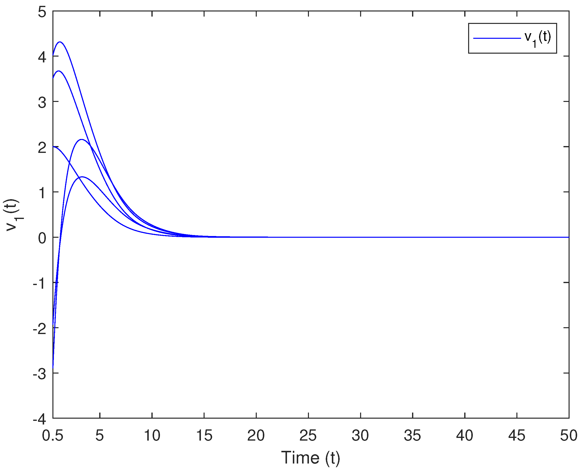
4. Simulation Example

In this section, one numerical example is shown to demonstrate the previous theoretical results. Consider the following NINNs with PDs and leakage delays.

$$\begin{array}{c}\left\{\begin{array}{cc}{v}_1^{″}\left(t\right)=\hfill & -\left(1+\frac{1}{25}sint\right)v_1^{\prime }\left(t\right)-\left(\frac{1}{4}+\frac{1}{50}cost\right)v_1(t-\frac{\left|sin(t-1)\right|}{10})+\frac{1}{10}cost{\tilde{f}}_1\left(v_1\left(t\right)\right)\hfill \\ \hfill & +\frac{1}{50}cost{\tilde{f}}_2\left(v_2\left(t\right)\right)+\frac{1}{10}{e}^{-\frac{1}{2}t}\left[{\tilde{g}}_1\left(v_1\left(\frac{1}{2}t\right)\right)+{\tilde{g}}_2\left(v_2\left(\frac{1}{2}t\right)\right)\right]\hfill \\ \hfill & +\frac{1}{15}{e}^{-\frac{1}{2}t}\left[{\tilde{h}}_1\left(v_1^{\prime }\left(\frac{1}{2}t\right)\right)\right.+{\tilde{h}}_2\left(v_2^{\prime }\left(\frac{1}{2}t\right)\right]+e^{-t}sint,\hfill \\ v_2^{″}\left(t\right)=\hfill & -\left(1+\frac{1}{25}cost\right)v_2^{\prime }\left(t\right)-\left(\frac{1}{4}+\frac{1}{50}sint\right)v_2(t-\frac{\left|sin(t-1)\right|}{20})+\frac{1}{10}sint{\tilde{f}}_1\left(v_1\left(t\right)\right)\hfill \\ \hfill & +\frac{1}{50}sint{\tilde{f}}_2\left(v_2\left(t\right)\right)+\frac{1}{10}{e}^{-\frac{1}{2}t}\left[{\tilde{g}}_1\left(v_1\left(\frac{1}{2}t\right)\right)+{\tilde{g}}_2\left(v_2\left(\frac{1}{2}t\right)\right)\right]\hfill \\ \hfill & +\frac{1}{15}{e}^{-\frac{1}{2}t}\left[{\tilde{h}}_1\left(v_1^{\prime }\left(\frac{1}{2}t\right)\right)\right.+{\tilde{h}}_2\left(v_2^{\prime }\left(\frac{1}{2}t\right)\right]+e^{-t}cost,\hfill \end{array}\right.\hfill \end{array}$$

(36)

where $t\ge t_0=1,{\tilde{f}}_j\left(x\right)=\frac{1}{18}x,{\tilde{g}}_j\left(x\right)=\frac{1}{18}sinx,{\tilde{h}}_j\left(x\right)=\frac{1}{6}sinx.$ Furthermore, we choose the following coefficients

$$\begin{array}{c}\begin{array}{cc}\hfill & {\rho }_{ij}={\gamma }_{ij}=\frac{1}{2},a_1\left(t\right)=1+\frac{1}{25}sint,a_2\left(t\right)=1+\frac{1}{25}cost,b_1\left(t\right)=\frac{1}{4}+\frac{1}{50}cost,\hfill \\ & b_2\left(t\right)=\frac{1}{4}+\frac{1}{50}sint,d_{11}\left(t\right)=\frac{1}{10}cost,d_{12}\left(t\right)=\frac{1}{50}cost,d_{21}\left(t\right)=\frac{1}{10}sint,d_{22}\left(t\right)=\frac{1}{50}sint,\hfill \\ \hfill & c_{11}\left(t\right)=c_{12}\left(t\right)=c_{21}\left(t\right)=c_{22}\left(t\right)=\frac{1}{10}{e}^{-\frac{1}{2}t},l_{11}\left(t\right)=l_{12}\left(t\right)=l_{21}\left(t\right)=l_{22}\left(t\right)=\frac{1}{15}{e}^{-\frac{1}{2}t},\hfill \\ \hfill & J_1\left(t\right)=e^{-t}sint,J_2\left(t\right)=e^{-t}cost,{\lambda }_1\left(t\right)=\frac{\left|sin(t-1)\right|}{10},{\lambda }_2\left(t\right)=\frac{\left|sin(t-1)\right|}{20}.\hfill \end{array}\hfill \end{array}$$

Through variable transformation, the above system can be rewritten as

$$\begin{array}{c}\left\{\begin{array}{cc}{v}_1^{\prime }\left(t\right)=\hfill & -\frac{1}{2}{v}_1\left(t\right)+u_1\left(t\right),\hfill \\ u_1^{\prime }\left(t\right)=\hfill & -(\frac{1}{2}+\frac{1}{25}sint)u_1\left(t\right)+\frac{1}{50}(sint-cost)v_1\left(t\right)+(\frac{1}{4}+\frac{1}{50}cost)v_1\left(t\right)\hfill \\ \hfill & -(\frac{1}{4}+\frac{1}{50}cost)v_1(t-\frac{\left|sin(t-1)\right|}{10})+\frac{1}{180}{v}_1\left(t\right)cost+\frac{1}{900}{v}_2\left(t\right)cost+\frac{1}{180}{e}^{-\frac{1}{2}t}\hfill \\ \hfill & \times [sin\left(v_1\left(\frac{1}{2}t\right)\right)+sin\left(v_2\left(\frac{1}{2}t\right)\right)]+\frac{1}{90}{e}^{-\frac{1}{2}t}[sin(v_1^{\prime }\left(\frac{1}{2}t\right))+sin(v_2^{\prime }\left(\frac{1}{2}t\right)\left)\right]+e^{-t}sint,\hfill \\ v_2^{\prime }\left(t\right)=\hfill & -\frac{1}{2}{v}_2\left(t\right)+u_2\left(t\right),\hfill \\ u_2^{\prime }\left(t\right)=\hfill & -(\frac{1}{2}+\frac{1}{25}cost)u_2\left(t\right)-\frac{1}{50}(sint-cost)v_2\left(t\right)+(\frac{1}{4}+\frac{1}{50}sint)v_2\left(t\right)\hfill \\ \hfill & -(\frac{1}{4}+\frac{1}{50}sint)v_2(t-\frac{\left|sin(t-1)\right|}{20})+\frac{1}{180}sint[v_1\left(t\right)+\frac{1}{5}{v}_2\left(t\right)]\hfill \\ \hfill & +\frac{1}{180}{e}^{-\frac{1}{2}t}sin\left(v_1\left(\frac{1}{2}t\right)\right)+\frac{1}{10}{e}^{-\frac{1}{2}t}\frac{1}{18}sin\left(v_2\left(\frac{1}{2}t\right)\right)\hfill \\ \hfill & +\frac{1}{15}{e}^{-\frac{1}{2}t}\frac{1}{6}sin(v_1^{\prime }\left(\frac{1}{2}t\right))+\frac{1}{15}{e}^{-\frac{1}{2}t}\frac{1}{6}sin(v_2^{\prime }\left(\frac{1}{2}t\right))+e^{-t}cost.\hfill \end{array}\right.\hfill \end{array}$$

(37)

It can be seen that

$$\begin{array}{cc}\hfill & p_1\left(t\right)=\frac{1}{2}+\frac{1}{25}sint,p_2\left(t\right)=\frac{1}{2}+\frac{1}{25}cost,\hfill \\ \hfill & k_1\left(t\right)=\frac{1}{50}(sint-cost),k_2\left(t\right)=-\frac{1}{50}(sint-cost).\hfill \end{array}$$

Noting that

$$\left|\frac{1}{18}x\right|\le \frac{1}{18}\left|x\right|,\left|\frac{1}{18}sinx\right|\le \frac{1}{18}\left|sinx\right|,\left|\frac{1}{6}sinx\right|\le \frac{1}{6}\left|sinx\right|,$$

and

$$e^{-{\int }_s^t{p}_i\left(\theta \right)d\theta }\le 1.1·e^{-\frac{23}{50}(t-s)},$$

we can acquire the result that

$${\delta }_1={\delta }_2=\frac{1}{2},L_j^{\tilde{f}}=L_j^{\tilde{g}}=\frac{1}{18},L_j^{\tilde{h}}=\frac{1}{6},{\overline{p}}_i=\frac{23}{50},M_i=1.05>1,i,j\in \{1,2\}.$$

Furthermore, we can select

$${\beta }_0=1,{\eta }_1={\eta }_2=\frac{1}{2},{\xi }_1={\xi }_2=2.$$

Accordingly, we can compute that

$$\begin{array}{cc}\hfill G_1\left(t\right)=& {\eta }_1^{-1}{\xi }_1|k_1\left(t\right)|+{\eta }_1^{-1}|b_1\left(t\right)|{\lambda }_1^{+}{e}^{{\beta }_0{\lambda }_1^{+}}+{\eta }_1^{-1}|d_{11}\left(t\right)|L_1^{\tilde{f}}{\xi }_1+{\eta }_1^{-1}|d_{12}\left(t\right)|L_2^{\tilde{f}}{\xi }_2\hfill \\ \hfill & +{\eta }_1^{-1}|c_{11}\left(t\right)|L_1^{\tilde{g}}{\xi }_1{e}^{{\beta }_0(1-{\rho }_{11})t}+{\eta }_1^{-1}|c_{12}\left(t\right)|L_2^{\tilde{g}}{\xi }_2{e}^{{\beta }_0(1-{\rho }_{12})t}\hfill \\ \hfill & +{\eta }_1^{-1}|l_{11}\left(t\right)|L_1^{\tilde{h}}{\xi }_1{e}^{{\beta }_0(1-{\gamma }_{11})t}+{\eta }_1^{-1}|l_{12}\left(t\right)|L_2^{\tilde{h}}{\xi }_2{e}^{{\beta }_0(1-{\gamma }_{12})t}\hfill \\ \hfill =& \frac{2}{25}|sint-cost|+\frac{|sin(t-1)|}{20}·e^{\frac{|sin(t-1)|}{10}}+\frac{|sin(t-1)|}{250}·|cost|·e^{\frac{|sin(t-1)|}{10}}\hfill \\ \hfill & +\frac{6}{225}|cost|+\frac{6}{45}\hfill \\ \hfill \le & \frac{2}{25}·2+\frac{1}{20}·e^{\frac{1}{10}}+\frac{1}{250}·1·e^{\frac{1}{10}}+\frac{6}{225}+\frac{6}{45}\hfill \\ \hfill \le & 0.32+0.054·e^{\frac{1}{10}}\approx 0.3797;\hfill \\ \hfill G_2\left(t\right)=& {\eta }_2^{-1}{\xi }_2|k_2\left(t\right)|+{\eta }_2^{-1}|b_2\left(t\right)|{\lambda }_2^{+}{e}^{{\beta }_0{\lambda }_2^{+}}+{\eta }_2^{-1}|d_{21}\left(t\right)|L_1^{\tilde{f}}{\xi }_1+{\eta }_2^{-1}|d_{22}\left(t\right)|L_2^{\tilde{f}}{\xi }_2\hfill \\ \hfill & +{\eta }_2^{-1}|c_{21}\left(t\right)|L_1^{\tilde{g}}{\xi }_1{e}^{{\beta }_0(1-{\rho }_{21})t}+{\eta }_2^{-1}|c_{22}\left(t\right)|L_2^{\tilde{g}}{\xi }_2{e}^{{\beta }_0(1-{\rho }_{22})t}+\hfill \\ \hfill & {\eta }_2^{-1}|l_{21}\left(t\right)|L_1^{\tilde{h}}{\xi }_1{e}^{{\beta }_0(1-{\gamma }_{21})t}+{\eta }_2^{-1}|l_{22}\left(t\right)|L_2^{\tilde{h}}{\xi }_2{e}^{{\beta }_0(1-{\gamma }_{22})t}\hfill \\ \hfill =& \frac{2}{25}|sint-cost|+\frac{|sin(t-1)|}{40}·e^{\frac{|sin(t-1)|}{20}}+\frac{|sin(t-1)|}{500}·|cost|·e^{\frac{|sin(t-1)|}{20}}\hfill \\ \hfill & +\frac{6}{225}|sint|+\frac{6}{45}\hfill \\ \hfill \le & \frac{2}{25}·2+\frac{1}{40}·e^{\frac{1}{20}}+\frac{1}{250}·1·e^{\frac{1}{20}}+\frac{6}{225}+\frac{6}{45}\hfill \\ \hfill \le & 0.32+0.027·e^{\frac{1}{20}}\approx 0.3484.\hfill \end{array}$$

It can be verified that

$$-{\delta }_i+\frac{{\eta }_i}{{\xi }_i}<0,{\delta }_i+\frac{{\eta }_i}{{\xi }_i}<1,i=1,2.$$

and

$$\begin{array}{c}{G}_i\left(t\right)<0.38,sup\{-{\overline{p}}_i+M_i{G}_i\left(t\right)\}=-0.46+0.38\ast 1.05=-0.061<0.\hfill \end{array}$$

Hence, assumptions $\left(H_1\right)$, $\left(H_2\right)$, and $\left(H_3\right)$ hold. By virtue of Theorem 1, it follows that any solution to the above equations converge exponentially to the equilibrium point.

Remark 7.

Obviously, Figure 1 and Figure 2 show that the numerical solutions exponentially converge to the zero vector as $t\to \infty$. Hence, the simulation results validate the proposed theoretical results well.

5. Conclusions

In this article, we consider the exponential stability for a class of NINNs with multi-proportional delays and leakage delays. In particular, by utilizing the variable transformation, the Lyapunov function approach, and the differential inequality technique, we have provided some sufficient conditions that ensure the global exponential stability of NINNs. Furthermore, the numerical behavior is in accordance with the theoretical findings. In the future, the stability of quaternion-valued NINNs with PDs and the synchronization issue of coupled inertial neural networks with PDs using various control strategies are worthy of further investigation.

References

1. Carpetern, G.A. Neural network models for patten recognition and associative memory. Neural Netw. 1989, 2, 243–257. [Google Scholar]
2. Cohen, M.; Grossberg, S. Absolute stability of global pattern formation and parallel memory storage by competive neural networks. IEEE Trans. Syst. Man Cybern. Syst. 1983, 13, 815–826. [Google Scholar] [CrossRef]
3. Chen, Y.; Zhang, N.; Chen, J. A survey of recent advances on stability analysis, state estimation and synchronization control for neural networks. Neurocomputing 2023, 515, 26–36. [Google Scholar] [CrossRef]
4. Babcock, K.; Westervelt, R. Dynamics of simple electronic neural networks. Phys. D 1987, 28, 305–316. [Google Scholar] [CrossRef]
5. Angelaki, D.E.; Correia, M.J. Models of membrane resonance in pigeon semicircular canal type II hair cells. Biol. Cybern. 1991, 65, 1–10. [Google Scholar] [CrossRef] [PubMed]
6. Wheeler, D.W.; Schieve, W.C. Stability and chaos in an inertial two-neuron system. Phys. D 1997, 105, 267–284. [Google Scholar] [CrossRef]
7. Duan, L.; Li, J. Fixed-time synchronization of fuzzy neutral-type BAM memristive inertial neural networks with proportional delays. Inf. Sci. 2021, 576, 522–541. [Google Scholar] [CrossRef]
8. Kong, F.; Zhu, Q.; Huang, T. Fixed-Time stability for discontinuous uncertain inertial neural networks with time-varying delays. IEEE Trans. Syst. Man Cybern. 2022, 52, 4507–4517. [Google Scholar] [CrossRef]
9. Zhou, L.; Zhu, Q.; Huang, T. Global polynomial synchronization of proportional delayed inertial neural networks. IEEE Trans. Syst. Man Cybern. 2023, in press. [CrossRef]
10. Wang, J.; Zhang, X.; Wang, X.; Yang, X. L2L state estimation of the high-order inertial neural network with time-varying delay: Non-reduced order strategy. Inf. Sci. 2022, 607, 62–78. [Google Scholar] [CrossRef]
11. Zhang, G.; Zeng, Z. Stabilization of second-order memristive neural networks with mixed time delays via nonreduced order. IEEE Trans. Neural Netw. Learn. Syst. 2020, 31, 700–706. [Google Scholar] [CrossRef] [PubMed]
12. Cui, N.; Jiang, H.; Hu, C.; Abdurahman, A. Global asymptotic and robust stability of inertial neural networks with proportional delays. Neurocomputing 2018, 272, 326–333. [Google Scholar] [CrossRef]
13. Li, Q.; Zhou, L. Global polynomial stabilization of proportional delayed inertial memristive neural networks. Inf. Sci. 2023, 623, 729–747. [Google Scholar] [CrossRef]
14. Long, C.; Zhang, G.; Zeng, Z.; Hu, J. Finite-time stabilization of complex-valued neural networks with proportional delays and inertial terms: A non-separation approach. Neural Netw. 2022, 148, 86–95. [Google Scholar] [CrossRef]
15. Kong, F.; Ren, Y.; Sakthivel, R. New criteria on periodicity and stabilization of discontinuous uncertain inertial Cohen-Grossberg neural networks with proportional delays. Chaos Solitons Fractals 2021, 150, 1–12. [Google Scholar] [CrossRef]
16. Aouiti, C.; Sakthivel, R.; Touati, F. Global dissipativity of fuzzy cellular neural networks with inertial term and proportional delays. Int. J. Syst. Sci. 2020, 51, 1392–1405. [Google Scholar] [CrossRef]
17. Guo, R.; Xu, S.; Guo, J. Sliding-mode synchronization control of complex-valued inertial neural networks with leakage delay and time-varying delays. IEEE Trans. Syst. Man Cybern. 2023, 53, 1095–1103. [Google Scholar]
18. Hale, J.K.; Lunel, S.M.V. Introduction to Function Differential Equation; Springer: Berlin, Germany, 1991. [Google Scholar]
19. Li, X. Global robust stability for stochastic interval neural networks with continuously distributed delays of neutral type. Appl. Math. Comput. 2010, 215, 4370–4384. [Google Scholar] [CrossRef]
20. Zhao, Y.; Zhu, Q. Stabilization of stochastic highly nonlinear delay systems with neutral-term. IEEE Trans. Autom. Control 2023, 68, 2544–2551. [Google Scholar] [CrossRef]
21. Lakshmanana, S.; Lima, C.P.; Prakashb, M.; Nahavandia, S.; Balasubramaniamc, P. Neutral-type of delayed inertial neural networks and their stability analysis using the LMI approach. Neurocomputing 2017, 230, 243–250. [Google Scholar] [CrossRef]
22. Duan, L.; Duan, J. Global lagrange stability of inertial neutral type neural networks with mixed time-varying delays. Neural Process Lett. 2020, 51, 1849–1867. [Google Scholar] [CrossRef]
23. Tu, Z.; Cao, J.; Alsaedi, A.; Alsaadi, F. Global dissipativity of memristor-based neutral type inertial neural networks. Neural Netw. 2017, 88, 125–133. [Google Scholar] [CrossRef] [PubMed]
24. Wu, K.; Jian, J. Non-reduced order strategies for global dissipativity of memristive neutral-type inertial neural networks with mixed time-varying delays. Neurocomputing 2021, 436, 174–183. [Google Scholar] [CrossRef]
25. Aouiti, C.; Hui, Q.; Jallouli, H.; Moulay, E. Fixed-time stabilization of fuzzy neutral-type inertial neural networks with time-varying delay. Fuzzy Sets Syst. 2011, 411, 48–67. [Google Scholar] [CrossRef]
26. Duan, L.; Li, J. Global exponential bipartite synchronization for neutral memristive inertial coupling mixed time-varying delays neural networks with antagonistic interactions. Commun. Nonlinear Sci. Numer. Simul. 2023, 119, 107071. [Google Scholar] [CrossRef]
27. Yu, Y. Global exponential convergence for a class of HCNNs with neutral time-proportional delays. Appl. Math. Comput. 2016, 285, 1–7. [Google Scholar] [CrossRef]
28. Xu, C.; Li, P. Global exponential convergence of neutral-type Hopfield neural networks with multi-proportional delays and leakage delays. Chaos Solitons Fractals 2017, 96, 139–144. [Google Scholar] [CrossRef]
29. Yang, G.; Wang, W. New results on convergence of CNNs with neutral type proportional delays and D operator. Neural Process Lett. 2019, 49, 321–330. [Google Scholar] [CrossRef]
30. Huang, C.; Su, R.; Cao, J.; Xiao, S. Asymptotically stable high-order neutral cellular neural networks with proportional delays and D operators. Math. Comput. Simul. 2020, 171, 127–135. [Google Scholar] [CrossRef]
31. Deng, Y.; Huang, C.; Cao, J. New results on dynamics of neutral type HCNNs with proportional delays. Math. Comput. Simul. 2021, 187, 51–59. [Google Scholar] [CrossRef]
32. Song, Q.; Yang, L.; Liu, Y.; Alsaadi, F.E. Stability of quaternion-valued neutral-type neural networks with leakage delay and proportional delays. Neurocomputing 2021, 521, 191–198. [Google Scholar] [CrossRef]
33. Jian, J.; Duan, L. Finite-time synchronization for fuzzy neutral-type inertial neural networks with time-varying coefficients and proportional delays. Fuzzy Sets Syst. 2020, 381, 51–67. [Google Scholar] [CrossRef]
34. Zhang, J.; Chang, A.; Yang, G. Periodicity on neutral-type inertial neural networks incorporating multiple delays. Symmetry 2021, 13, 2231. [Google Scholar] [CrossRef]
35. Zhang, A. Almost periodic solutions for SICNNs with neutral type proportional delays and D operators. Neural Process. Lett. 2018, 47, 57–70. [Google Scholar] [CrossRef]
36. Li, B.; Cao, Y.; Li, Y. Almost periodic oscillation in distribution for octonion-valued neutral-type stochastic recurrent neural networks with D operator. Nonlinear Dyn. 2023, 111, 11371–11388. [Google Scholar] [CrossRef]
37. Rao, R.; Lin, Z.; Ai, X.; Wu, J. Synchronization of epidemic systems with Neumann boundary value under delayed impulse. Mathematics 2022, 10, 2064. [Google Scholar] [CrossRef]
38. Li, G.; Zhang, Y.; Guan, Y.; Li, W. Stability analysis of multi-point boundary conditions for fractional differential equation with non-instantaneous integral impulse. Math. Biosci. Eng. 2023, 20, 7020–7041. [Google Scholar] [CrossRef]
39. Zhao, Y.; Wang, L. Practical exponential stability of impulsive stochastic food chain system with time-varying delays. Mathematics 2023, 11, 147. [Google Scholar] [CrossRef]
40. Xia, M.; Liu, L.; Fang, J.; Zhang, Y. Stability analysis for a class of stochastic differential equations with impulses. Mathematics 2023, 11, 1541. [Google Scholar] [CrossRef]
41. Tang, Y.; Zhou, L.; Tang, J.; Rao, Y.; Fan, H.; Zhu, J. Hybrid impulsive pinning control for mean square Synchronization of uncertain multi-link complex networks with stochastic characteristics and hybrid delays. Mathematics 2023, 11, 1697. [Google Scholar] [CrossRef]
42. Li, K.; Li, R.; Cao, L.; Feng, Y.; Onasanya, B.O. Periodically intermittent control of memristor-based hyper-chaotic bao-like system. Mathematics 2023, 11, 1264. [Google Scholar] [CrossRef]
43. Wang, C.; Liu, X.; Jiao, F.; Mai, H.; Chen, H.; Lin, R. Generalized Halanay inequalities and relative application to time-delay dynamical systems. Mathematics 2023, 11, 1940. [Google Scholar] [CrossRef]
44. Xue, Y.; Han, J.; Tu, Z.; Chen, X. Stability analysis and design of cooperative control for linear delta operator system. AIMS Math. 2023, 8, 12671–12693. [Google Scholar] [CrossRef]
45. Zhu, Q. Stabilization of stochastic nonlinear delay systems with exogenous disturbances and the event-triggered feedback control. IEEE Trans. Autom. Control 2019, 64, 3764–3771. [Google Scholar] [CrossRef]
46. Zhu, Q.; Huang, T. H control of stochastic networked control systems with time-varying delays: The event-triggered sampling case. Int. J. Robust Nonlinear Control 2021, 31, 9767–9781. [Google Scholar] [CrossRef]
Figure 1. Numerical solutions to Example 1 with initial values ( φ 1 , φ 2 ) = ( 2 , 3 ) , (4, 2), (−3, −2), (−2, −1.5), (3.5, −1.2): time series of v 1 .
Mathematics 11 02596 g001
Figure 2. Numerical solutions to Example 1 with initial value ( φ 1 , φ 2 ) = ( 2 , 3 ) , (4, 2), (−3, −2), (−2, −1.5), (3.5, −1.2): time series of v 2 .
Mathematics 11 02596 g002
Disclaimer/Publisher’s Note: The statements, opinions and data contained in all publications are solely those of the individual author(s) and contributor(s) and not of MDPI and/or the editor(s). MDPI and/or the editor(s) disclaim responsibility for any injury to people or property resulting from any ideas, methods, instructions or products referred to in the content.