A Frequency Attention-Based Dual-Stream Network for Image Inpainting Forensics

Abstract

The rapid development of digital image inpainting technology is causing serious hidden danger to the security of multimedia information. In this paper, a deep network called frequency attention-based dual-stream network (FADS-Net) is proposed for locating the inpainting region. FADS-Net is established by a dual-stream encoder and an attention-based blue-associative decoder. The dual-stream encoder includes two feature extraction streams, the raw input stream (RIS) and the frequency recalibration stream (FRS). RIS directly captures feature maps from the raw input, while FRS performs feature extraction after recalibrating the input via learning in the frequency domain. In addition, a module based on dense connection is designed to ensure efficient extraction and full fusion of dual-stream features. The attention-based associative decoder consists of a main decoder and two branch decoders. The main decoder performs up-sampling and fine-tuning of fused features by using attention mechanisms and skip connections, and ultimately generates the predicted mask for the inpainted image. Then, two branch decoders are utilized to further supervise the training of two feature streams, ensuring that they both work effectively. A joint loss function is designed to supervise the training of the entire network and two feature extraction streams for ensuring optimal forensic performance. Extensive experimental results demonstrate that the proposed FADS-Net achieves superior localization accuracy and robustness on multiple datasets compared to the state-of-the-art inpainting forensics methods.

1. Introduction

With the rapid development of digital image processing techniques, increasingly advanced image editing software provides more convenience and fun for modern human life. Nevertheless, a large number of forged digital images are generated by malicious use of these techniques, which has led to a serious security and trust crisis of digital multimedia. Therefore, image forensics has gradually attracted an increasing concern in the digital multimedia era, such as JPEG compression forensics [1,2], median filtering detection [3], copy-moving and splicing localization [4,5], universal image manipulation detection [6,7], and so on.

Image inpainting is an effective image editing technique which aims to repair damage or removed image regions based on known image information in a visually plausible manner, as shown in Figure 1. A variety of image inpainting methods have been constantly proposed in recent years, and these can be classified roughly into three categories: the diffusion-based approaches [8,9], the exemplar-based approaches [10,11], and the deep learning (DL)-based approaches [12,13]. Due to its effective and efficient editing ability, image inpainting has been widely applied in many image processing fields [11], such as image restoration, image coding and transmission, photo-editing and virtual restoration of digitized paintings, etc. However, the powerful image editing tool is also conveniently used to maliciously modify an image even by non-professional forgers with less visible traces, which poses a serious threat to multimedia information security.

The major forensic tasks for image inpainting are to locate the inpainted regions of an input image, so inpainting forensics require pixel-wise binary classification at the manipulation level, i.e., binary semantic segmentation. In fact, the goal of binary semantic segmentation is to classify pixels in an image into two categories: foreground and background. Specifically, for the inpainting forensics task, the pixels in the image are classified into inpainted pixels and uninpainted pixels. Generally, this is more difficult than the common manipulation detection, which only makes a decision regarding whether a certain manipulation took place or not.

There has been limited research on inpainting forensics until now. Some traditional forensic methods employ hand-crafted features to identify inpainted pixels. For instance, the features depending on image patch similarity were extracted for the detection of exemplar-based inpainting operation [14,15], and the features based on image Laplacian transform were designed to identify the diffusion-based inpainting operation [16,17]. However, the manipulation traces left by image inpainting on the image are so weak that it is hard to reveal by manually designed features. In addition, the emerging DL-based inpainting methods can not only achieve more realistic inpainting results than traditional methods, but also generate new objects, which brings greater challenges to inpainting forensics. Recently, deep convolutional neural networks (DCNNs) have made great success in many fields [18,19,20] via their powerful learning capabilities. Inspired by these works, some researchers have made some attempts to develop CNN-based forensics methods, such as median filtering forensics [3], camera model identification [21], copy-move and splicing localization [4], as well as JPEG compression forensics [2]. A few research efforts have been also devoted to deep learning-based forensics for image inpainting [22,23].

DL-based methods learn the discriminant features and make the decisions for target tasks in a data-driven way and thus bring about a significant performance advantage on large-scale datasets. In this paper, we propose a new end-to-end network for image inpainting forensics. The network is established by considering the following factors.

First, manipulation feature extraction is a key problem for the DL-based inpainting forensics. Although DCNN is employed to directly extract features from the inpainted image through end-to-end training [22,24], it tends to learn image content rather than manipulate features [25]. To this end, the preprocessing modules are constructed to enhance image manipulation traces in many deep forensic approaches [7,23,26]. However, most of these methods rely on prior knowledge and cannot be effectively applied to all inpainting methods.

In addition, down-sampling operations are inevitably used in a DCNN for the extraction of high-level features, causing detail information loss on image regions [27]. For dense prediction forensics, it is necessary to study the strategies for compensating spatial information.

Last, cross-entropy and weighting strategies are generally selected for most deep inpainting forensics [23,24,26]. In practice, the loss function is extremely important for training DL-based methods, and its selection should be closely related to the proposed network structure and mission objectives. Thus, the design of loss function needs to be carefully considered based on our methods.

Based on the above considerations, we propose a novel dual-stream network for image inpainting forensics, called frequency attention-based dual-stream network (FADS-Net) in this paper. The main contributions of this work are three-fold, as below:

• We develop the DCNN for image inpainting forensics following the encoder–decoder network structure [18,28] to directly regress the ground truth binary mask, representing the pixel-wise class labels (inpainting and uninpainting). In order to capture richer inpainting clues, the encoder is designed as a dual-stream structure that consists of the raw input stream (RIS), the frequency recalibration stream (FRS), and a fusion module. The RIS, like most forensics methods, takes the original inpainted image as the input, and image information adaptively recalibrated in the frequency domain is used as input to the FRS. Then, the extracted dual-streamed features are fused into more effective and comprehensive feature responses through a well-designed fusion module. Finally, the fused features will be gradually enlarged to the full resolution through the decoder, and the final prediction mask is generated.
• We design the comprehensive up-sampling module combining transpose convolution [29], skip connection [30], and attention mechanism [31]. Through transpose convolution, the fed features are refined to enhance the feature representations for the purpose of forensics while increasing the feature resolution. Information fusion can be effectively performed between coarse high-level features and fine low-level features by combination of skip connection and attention mechanism, which compensates for the spatial information loss caused by the down-sampling operations in the encoder.
• We design a new joint loss function based on the intersection-over-union (IoU) metric to train the proposed forensics network. The loss is obtained by combining a proposed IoU loss and the cross entropy (CE) loss, where the IoU loss can directly guide the FADS-Net to optimize the IoU performance metric. CE loss is used to supervise the training of the entire network and two feature extraction streams, respectively, which ensures stable training of the network and efficient operation of each feature extraction stream.

The structure of this paper is as follows. Section 2 briefly introduces the related work of inpainting forensics. In Section 3, a frequency attention-based dual-stream forensics network is proposed and details of the network are presented. A series of experiments are carried out to evaluate the proposed network in Section 4. Finally, Section 5 concludes this paper.

2. Related Works

A few research efforts have been devoted to developing forensic methods for image inpainting. They can be roughly divided into the following two categories.

2.1. Conventional Inpainting Forensics Methods

The conventional inpainting forensic methods rely on manually designed features to predict the inpainted pixels. Initially, for exemplar-based inpainting [10], a zero-connectivity length (ZCL) feature was designed to measure the similarity among image patches, and the inpainted patches were recognized by a fuzzy membership function of patch similarity [32]. A similar forensics method depending on patch similarity was presented in [33] for video inpainting. However, the similar patch searching process is very time-consuming, especially for a large image. In addition, a high false alarm rate may be provided by these methods for an image with uniform background.

The skipping patch matching was explored for inpainting forensics and copy-move detection in [34]. A two-stage patch searching method based on weight transformation was proposed in [14]. The two patch search methods accelerate the search of suspicious patches, but may cause accuracy loss. Furthermore, by multi-region relations based ZCL features, the inpainted image regions are identified in [14], achieving an improved false alarm rate. The work was further improved by exploiting the greatest ZCL feature and fragment splicing detection in [15]. Meanwhile, the suspicious patch search was sped up by the central pixel mapping method. The resulting problem is that a truly inpainted region is prone to be recognized as some isolated suspicious regions and they might be removed by fragment splicing detection.

The inpainted patch set was determined by the hybrid feature including Euclidean distance, the position distance, and the number of same pixels between two image patches in [35]. Unfortunately, the feature is very weak against the image post-processing operations and the forensics performance is highly image-dependent.

A few works were dedicated to improving the robustness of the inpainting forensics. For the compressed inpainted image, the forensics was performed by computing and segmenting the averaged sum of absolute difference images between the target image and a resaved JPEG compressed image at different quality factors [36]. However, the feature effectiveness is not clear if the image samples are modified using other manipulations. The method in [37] was developed based on high-dimensional feature mining in the discrete cosine transform domain to resist the compression attack. Many combinations of inpainting, compression, filtering, and resampling are recognized by extracting the marginal density and neighboring joint density features in [38]. The obtained classifiers only distinguish the considered specific forgery methods and do not locate the inpainted region.

To detect image tampering by sparsity-based image inpainting schemes [39,40], the forensics method based on canonical correlation analysis (CCA) was proposed in [41]. The method exhibits the advantage of robustness against some image post-processing operations, but has the same drawback as [38]. For diffusion-based inpainting technologies [8,9], a feature set based on the image Laplacian was constructed to identify the inpainted regions in [16]. The performance was further enhanced by weighted least squares filtering and the ensemble classifier in [17]. However, these methods fail to resist even quite weak attacks.

Principally, hand-crafted features for image inpainting are designed according to the observations in some images, which cannot be guaranteed to be valid in all cases. Moreover, the design of robust hand-crafted features is usually very difficult, since no obvious traces are left by image inpainting operations, particularly deep learning-based inpainting methods. In addition, the optimization of classifiers is carried out on a relatively small dataset or in a certain small parameter range and is dependent upon feature extraction, causing the restricted forensic performance.

2.2. Deep Learning-Based Inpainting Forensics Methods

The strategy of the method based on deep learning is different from the conventional one, which can automatically learn the inpainting features and makes decisions in a data-driven way. As the first attempt in [22], the fully convolutional network (FCN) was constructed to locate the tampered regions by exemplar-based inpainting method [10], and the weighted CE loss was designed to tackle the imbalance between the inpainted and normal pixels. The method is significantly superior to the conventional forensics methods in terms of detection accuracy and robustness, which can be further improved by skip connections [42]. A deep learning approach combining CNN and long short-term memory (LSTM) network was proposed in [43] to accomplish the spatially dense prediction for exemplar-based inpainting. As to the network design, attention is mainly concentrated on the improvement of the robustness and false alarm performance. The ResNet-based approach [44] merged the networks of object detection and semantic segmentation. The approach is developed to achieve the hybrid forensic purpose for exemplar-based inpainting, including manipulated localization, recognition, and semantic segmentation. The forensic approach for deep inpainting was first addressed in [23], and an FCN with a high-pass filter was designed to identify the inpainted pixels in an image.

Recently, some of the latest advances in deep learning have also been applied to the design of inpainting forensics methods. A deep forensic network was proposed in [26] which is automatically designed through the one-shot neural structure search algorithm [45] and includes a preprocessing module to enhance inpainting traces. A backbone network with multi-stream structure [46] was employed to establish a progressive network for image manipulation detection and localization [24], which could gradually fine-tune the prediction results from low resolution to high resolution.

DL-based methods can learn the discriminant features directly from the data, avoiding the difficulties of manually extracting features. Moreover, relying on end-to-end learning, DCNNs permit the optimization of the feature extraction and the final decision steps in a unique framework. With these characteristics, DL-based methods manifest a significant performance advantage on large-scale datasets. This motivates us to further investigate the deep learning-based methods for inpainting forensics.

3. Frequency Attention-Based Dual-Stream Inpainting Forensics Network

In this section, a dual-stream inpainting forensics network based on attention in the frequency domain, abbreviated as FADS-Net in this paper, is presented. We build our forensic network based on the encoder–decoder network structure by considering the fact that such networks are widely used for dense prediction tasks and produce remarkable results [18,28]. The overall architecture of FADS-Net is illustrated in Figure 2. As shown in Figure 2, FADS-Net first encodes a given input image into feature maps by a dual-stream encoder and then sends features to an attention-based associative decoder to generate final predictions for the entire network and individual feature streams. The network is carefully designed by considering the network architecture, the main function modules, and the loss function, which are described in the following one by one.

3.1. Dual-Stream Encoder with Attention in Frequency Domain

The encoder part of the proposed network contains two branches of feature extraction: raw input stream (RIS) and frequency recalibrated stream (FRS). As feature extraction sub-networks with the same backbone structure, they are able to capture the features of the inpainting trace by utilizing their respective input information. The RIS learns manipulation features directly, which represent the difference between the inpainted and uninpainted regions, through the original image $\mathit{I}$, that is,

$${\mathit{X}}_{\mathrm{RIS}}={\mathcal{F}}_{\mathrm{RIS}}\left(\mathit{I}\right)$$

(1)

where composite function ${\mathcal{F}}_{\mathrm{RIS}}(·)$ represents the feature extraction operation performed by RIS. Meanwhile, the image ${\mathit{I}}_{\mathrm{FR}}$ recalibrated by a frequency-domain preprocessing module, called the adaptive frequency recalibration module (AFRM), serves as the input of another branch, namely the FRS. The overall process can be written as

$${\mathit{I}}_{\mathrm{FR}}={\mathcal{F}}_{\mathrm{AFR}}\left(\mathit{I}\right)$$

(2)

$${\mathit{X}}_{\mathrm{FRS}}={\mathcal{F}}_{\mathrm{FRS}}\left({\mathit{I}}_{\mathrm{FR}}\right)$$

(3)

where ${\mathcal{F}}_{\mathrm{AFR}}(·)$ represents the operation of the AFRM on the input image, and ${\mathcal{F}}_{\mathrm{FRS}}(·)$ is a composite function that represents the operation of extracting features from ${\mathit{I}}_{\mathrm{FR}}$ performed by FRS. The application of AFRM can enhance the inpainting traces and suppress irrelevant information through the data-driven method. The network backbones of the above two streams are constructed based on the single-stream CNN for inpainting forensics proposed in our other recent work (under submission). The feature responses extracted from the two feature streams are fully fused through a dual-stream feature fusion module (DFFM) to obtain more abundant and more effective inpainting feature representation, as follows:

$${\mathit{X}}_{\mathrm{DSF}}={\mathcal{F}}_{\mathrm{DFF}}({\mathit{X}}_{\mathrm{RIS}},{\mathit{X}}_{\mathrm{FRS}})$$

(4)

where ${\mathcal{F}}_{\mathrm{DFF}}(·,·)$ represents the feature fusion operation performed in DFFM.

A more detailed description of the AFRM, the network backbone of two feature extraction streams, and DFFM will be provided in the following sections.

3.1.1. Adaptive Frequency Recalibration Module

Some researchers attempt to combine manually designed features with DCNN [3,23,26] for further mining of latent artifacts. However, these prior knowledge-based methods are insufficient to capture comprehensive inpainting traces. Moreover, faced with the challenge of increasingly advanced inpainting technologies to forensic science, frequency-related features may provide extra and abundant forensic clues [3,47], except for the visual inpainting traces revealed in RGB space.

Based on the above considerations and inspired by [47,48], the adaptive frequency recalibration module is proposed to adaptively enhance frequency-related inpainting features through a data-driven approach. The process of this module is illustrated in Figure 3.

First, we attempt to employ discrete cosine transform (DCT) to convert the input inpainted image $\mathit{I}\in {\mathbb{R}}^{W\times H\times 3}$ from the spatial domain to frequency domain, where W and H denote the width and height of the image, respectively. Thanks to its positive decorrelation and excellent energy compaction, DCT has been applied extensively to the field of image processing. However, the complexity of DCT is relatively high, so the block-based DCT is usually selected to process images. Considering the computational cost, we apply 2-D DCT with a block of size $8\times 8$ (marked as $8\times 8$ DCT) to each channel of $\mathit{I}$. Thus, the DCT result $X_{\mathrm{d}}^{\left(i\right)}$ of the i-th channel ${\mathit{I}}^{\left(i\right)}$ can be expressed as

$$X_{\mathrm{d}}^{\left(i\right)}=\mathcal{D}\left({\mathit{I}}^{\left(i\right)}\right)$$

(5)

where $i\in \{1,2,3\}$, and $\mathcal{D}(·)$ indicates the $8\times 8$ DCT. Through applying $8\times 8$ DCT, there are a total of $W/8\times H/8$ blocks with size $8\times 8$ generated on each channel. As a result of converting to the frequency domain, all elements in each block represent the DCT coefficients of the corresponding frequency components, which are regularly distributed at various locations in each block according to the frequency.

Then, the 2-D DCT resulting on each RGB channel needs to be reshaped into a 3-D shape for further processing. Specifically, the components with the same frequency in all $8\times 8$ blocks of each channel are grouped into the same channel, and still maintain the spatial relationships with each other. In this way, each of the R, G, and B components of the inpainted image forms a tensor with 64 channels, which correspond to different frequencies. The overall reshaped result ${\mathit{X}}_{\mathrm{r}}\in {\mathbb{R}}^{W/8\times H/8\times 192}$ is achieved through concatenating these generated tensors. The above process can be expressed as

$${\mathit{X}}_{\mathrm{r}}=[\mathcal{R}\left({\mathit{X}}_{\mathrm{d}}^{\left(1\right)}\right),\mathcal{R}\left({\mathit{X}}_{\mathrm{d}}^{\left(2\right)}\right),\mathcal{R}\left({\mathit{X}}_{\mathrm{d}}^{\left(3\right)}\right)]$$

(6)

where $\mathcal{R}(·)$ and $[·]$ denote the reshaping and concatenating operations, respectively.

At present, each channel of ${\mathit{X}}_{\mathrm{r}}$ represents the different frequency information of an inpainted image. The inpainting manipulation fills the tampered region with known image information, which inevitably causes changes in energy in some frequency bands of the original image. To adaptively enhance the weak inpainting trace and suppress irrelevant information, we attempt to employ channel attention [49] to learn a frequency attention map ${\mathcal{M}}_{\mathrm{F}}$ of ${\mathit{X}}_{\mathrm{r}}$, which would be utilized to recalibrate information on different frequency bands of ${\mathit{X}}_{\mathrm{r}}$. To be specific, ${\mathit{X}}_{\mathrm{r}}$ is first converted into a global descriptor ${\mathcal{X}}_{\mathrm{F}}\in {\mathbb{R}}^{1\times 1\times 192}$ through the global average pooling (GAP) $\mathcal{G}(·)$, that is,

$${\mathcal{X}}_{\mathrm{F}}^{\left(k\right)}=\mathcal{G}\left(x_{\mathrm{r}}(i,j,k)\right)=\frac{1}{W/8\times H/8}\sum _{i=1}^{W/8}\sum _{j=1}^{H/8}{x}_{\mathrm{r}}(i,j,k)$$

(7)

where $x_{\mathrm{r}}(i,j,k)$ represents the DCT coefficient located at $(i,j)$ on the k-th channel of ${\mathit{X}}_{\mathrm{r}}$, and ${\mathcal{X}}_{\mathrm{F}}^{\left(k\right)}$ is the k-th element of ${\mathcal{X}}_{\mathrm{F}}$, which represents the global information of the k-th channel of ${\mathit{X}}_{\mathrm{r}}$. Then, the ${\mathcal{X}}_{\mathrm{F}}$ is input into a multi-layer perceptron (MLP) with the sigmoid function $\sigma (·)$ to derive ${\mathcal{M}}_{\mathrm{F}}$. The process can be expressed as

$${\mathcal{M}}_{\mathrm{F}}=\sigma \left({\mathit{W}}_2\delta \left({\mathit{W}}_1{\mathcal{X}}_F\right)\right)$$

(8)

where ${\mathit{W}}_1$ and ${\mathit{W}}_2$ denote the weight parameters of the hidden layer and output layer, respectively, of MLP, and $\delta (·)$ denotes a rectified linear unit (ReLU) activation function. Finally, the recalibrated frequency information ${\mathit{X}}_{\mathrm{r}}^{\prime }$ is achieved by

$${\mathit{X}}_{\mathrm{r}}^{\prime }={\mathcal{M}}_{\mathrm{F}}\otimes {\mathit{X}}_{\mathrm{r}}$$

(9)

where ⊗ refers to element-wise multiplication.

By applying the channel attention mechanism, the dynamic weight is provided for each frequency channel of ${\mathit{X}}_{\mathrm{r}}$, so as to improve the effectiveness of frequency information for forensics. However, the forensics network infers the final pixel-wise prediction, which depends on the spatial information of the image. Therefore, the recalibrated result ${\mathit{X}}_{\mathrm{r}}^{\prime }$ in the frequency domain is reconverted into an image ${\mathit{I}}_{\mathrm{FR}}$ in the spatial domain by inverse reshaping ${\mathcal{R}}^{-1}(·)$ and inverse DCT ${\mathcal{D}}^{-1}(·)$, which is implemented as follows:

$${\mathit{I}}_{\mathrm{FR}}=[{\mathcal{D}}^{-1}\left({\mathcal{R}}^{-1}\left({\mathit{X}}_{\mathrm{r}}^{{}^{\prime }\left(1\right)}\right)\right),{\mathcal{D}}^{-1}\left({\mathcal{R}}^{-1}\left({\mathit{X}}_{\mathrm{r}}^{{}^{\prime }\left(2\right)}\right)\right),{\mathcal{D}}^{-1}\left({\mathcal{R}}^{-1}\left({\mathit{X}}_{\mathrm{r}}^{{}^{\prime }\left(3\right)}\right)\right)]$$

(10)

where $[·]$ denotes the concatenating operation, and ${\mathit{X}}_{\mathrm{r}}^{{}^{\prime }\left(i\right)}$ is the recalibration result of the i-th channel of the input image $\mathit{I}$ through channel attention.

Although CNN has superior feature learning capabilities, it may be insufficient that only RIS is utilized to learn features of inpainting operation. This is because, in the spatial domain, the inpainting traces are hidden in the content information of an image, while CNN tends to learn the features of content information. According to the previous description, through DCT and reshaping, AFRM can first alleviate the coupling between image content and inpainting artifact, which have different frequency information in the frequency domain. Furthermore, channel attention is employed to adaptively enhance or suppress corresponding frequency information through data-driven approaches, so as to meet the requirement of forensic tasks. Therefore, the FRS can also extract extra abundant features from the images recorrected by AFRM, and these features extracted by FRS will be fused with the features obtained by RIS to ultimately improve the forensic performance. The comparative and ablation experiments have demonstrated the effectiveness of FRS with AFRM.

3.1.2. Sub-Network for High-Resolution Feature Extraction

In general, depending on the progressive down-sampling and deep structure, DCNN can learn abstract high-level features. However, the continuous down-sampling results in the serious loss of spatial details, which is harmful to the dense prediction task [50].

Thus, a network structure in Figure 2 proposed in our recent work is employed to establish the sub-networks of two feature extraction streams which can effectively extract high-resolution feature responses from their respective input information.

Thus, a single-stream network with the structure in Figure 2 proposed in our recent work is introduced as a sub-network to efficiently extract high-resolution feature responses. For readers to better understand our work, the network is re-described in the following.

At the beginning, a convolution block is employed to generate shallow feature maps from input information. Subsequently, the combination of down-sampling block and multi-stream dense modules (MSDMs) is repeatedly applied three times to further learn higher-level features. As a result, the spatial resolution of the final feature responses on each stream is adjusted to 1/8 of that of the input, which effectively reduces the loss of detail information on the inpainted regions.

As the basic unit of the network and the component of other modules, the convolution block implements the feature extraction through the convolution operations, followed by a batch normalization (BN) layer and ReLU activation layer.

By setting the stride to 2, the above convolution block is converted into a down-sampling block, so as to reduce the spatial resolution of input feature maps by half. Compared to ordinary prior-based pooling, this trainable down-sampling is more suitable for forensics tasks of learning inpainting trace rather than image content.

MSDM is the main unit and was designed in our recent work to efficiently learn feature representation after each down-sampling. It has three parallel information flows: local feature stream, global feature stream, and residual stream.

Through multiple densely connected dilated convolutional blocks, the local feature stream is employed to learn a set of local features from the input of MSDM. For the n-th dilated convolution block in the k-th MSDM, the local features ${\mathit{X}}_{\mathrm{L}}^{(k,n)}$ extracted by it can be expressed as

$${\mathit{X}}_{\mathrm{L}}^{(k,n)}={\mathcal{F}}_{\mathrm{DCB}}\left([{\mathit{X}}_{\mathrm{I}}^{\left(k\right)},{\mathit{X}}_{\mathrm{L}}^{(k,1)},\cdots ,{\mathit{X}}_{\mathrm{L}}^{(k,n-1)}]\right)$$

(11)

where ${\mathit{X}}_{\mathrm{I}}^{\left(k\right)}$ denotes the input feature of the k-th MSDM in the feature extractor, $[·]$ denotes the concatenating operation, and ${\mathcal{F}}_{\mathrm{DCB}}$ denotes the operation performed by the n-th convolutional block. Dense connection can not only strengthen information propagation and promote feature reuse, but also effectively improve model compactness [19,51,52].

Then, the global feature stream can aggregate the global context of input by global average pooling (GAP) $\mathcal{G}(·)$ to obtain the image-level features. For the k-th MSDM, the image-level features ${\mathit{X}}_{\mathrm{G}}^{\left(k\right)}$ can be obtained as follows:

$${\mathit{X}}_{\mathrm{G}}^{\left(k\right)}=\mathcal{U}\left(\mathcal{G}\left(\mathcal{C}\left({\mathit{X}}_{\mathrm{I}}^{\left(k\right)}\right)\right)\right)$$

(12)

where $\mathcal{C}(·)$ and $\mathcal{U}(·)$ represent convolution and up-sampling operations, respectively, which are used to adjust the dimensions of feature maps so as to facilitate subsequent feature fusion performed by MSDM.

Finally, the input features and local and global features are fused by a $1\times 1$ convolutional block, and the derived results as residuals are combined with the inputs of MSDM, forming the residual stream. When N densely connected convolutional blocks are set on the local feature stream of MSDM, the final output ${\mathit{X}}_{\mathrm{O}}^{\left(k\right)}$ of the k-th MSDM can be expressed as

$${\mathit{X}}_{\mathrm{O}}^{\left(k\right)}={\mathcal{F}}_{\mathrm{FCB}}\left([{\mathit{X}}_{\mathrm{I}}^{\left(k\right)},{\mathit{X}}_{\mathrm{L}}^{(k,1)},\cdots ,{\mathit{X}}_{\mathrm{L}}^{(k,N)},{\mathit{X}}_{\mathrm{G}}^{\left(k\right)}]\right)\oplus {\mathit{X}}_{\mathrm{I}}^{\left(k\right)}$$

(13)

where ${\mathcal{F}}_{\mathrm{FCB}}(·)$ and ⊕ refer to feature fusion performed by the $1\times 1$ convolutional block and pixel-wise addition, respectively. The detailed description of MSDM is provided in our recent work.

3.1.3. Dense-Scale Feature Fusion

The final feature responses ${\mathit{X}}_{\mathrm{RIS}}$ and ${\mathit{X}}_{\mathrm{FRS}}$ extracted from the two feature streams contain abundant and valid forensic information. We utilize a dense-scale feature fusion module (DFFM) to promote their full fusion and finally obtain a fusion feature representation ${\mathit{X}}_{\mathrm{DSF}}$.

The DFFM is composed of a convolution block and a specially set MSDM, as illustrated in Figure 4. Firstly, ${\mathit{X}}_{\mathrm{RIS}}$ and ${\mathit{X}}_{\mathrm{FRS}}$ are concatenated along the channel dimension. Then, a convolution block is used to resize the channel depth of the concatenated feature maps by a factor of 0.5, which can reduce the computation cost of subsequent processing. Furthermore, we employ the specially set MSDM (marked as MSDM${}_{\mathrm{DF}}$) to capture a set of dense-scale context information from the concatenated feature maps and then fuse them together, so as to promote the in-depth mining and interacting of feature maps on dense scales.

Specifically, for a dilated convolution layer with kernel size S and dilation rate $\lambda$, its receptive field R can be obtained by

$$R=S+(S-1)\times (\lambda -1)$$

(14)

Obviously, we can flexibly adjust the receptive fields R to incorporate different contexts by setting dilated rate $\lambda$. In addition, N dilated convolution blocks with the dense connection can form a total of ${\sum }_{i=1}^N{C}_N^i=2^N-1$ information propagation paths on local feature stream of MSDM${}_{\mathrm{DF}}$, where $C_N^i$ represents the number of all combinations of i elements taken from N different elements. Furthermore, when there are k convolution blocks on a path, a larger equivalent receptive field $R_e$ would be obtained.

$$R_e=\sum _{i=1}^k{R}_i-k+1$$

(15)

Hence, by adjusting the dilation rate of each dilated convolution block in MSDM, a set of receptive fields can be generated to capture contextual information with dense scales.

In this paper, we set the dilation rates in MSDM${}_{\mathrm{DF}}$ to 1, 2, 4 in order. According to the above design, the scale of the i-th local receptive field is $2i+1,i=1,\cdots ,7.$ Moreover, the purple plane represents the receptive field that aggregates the global context on the global feature stream, which can not only further enrich the feature information, but also effectively avoids the degradation of equivalent receptive fields caused by dilation rate settings [50]. Simulations indicate that the performance of the proposed network can be effectively improved by the proposed DFFM.

3.2. Attention-Based Associative Decoder

We propose an attention-based associative decoder, which consists of a main decoder and two branch decoders in parallel. The main decoder can gradually restore the spatial resolution of features and refine them, thereby yielding the final prediction for dense forensics. Moreover, two decoders with the same structure are applied on two individual feature streams, which is facilitated to further supervise their training and ensures that they both work effectively.

3.2.1. Main Decoder and Branch Decoder

The main decoder consists of up-sampling blocks, locality-sensitive attention modules (LSAMs), skip connection units, convolution blocks, and Softmax layer, as shown in Figure 2.

The up-sampling block resizes the resolution of the input feature maps by a factor of 2, which is constructed by replacing the convolutional layer with a transposed convolutional layer in the down-sampling block. Different from linear interpolation and inverse pooling, the up-sampling operation based on transposed convolution can learn feature representation with trainable parameters while increasing the feature resolution. This is obviously favorable for the forensic task.

A skip connection unit is usually directly arranged behind the up-sampling block, which can introduce the encoder features to compensate for the lost spatial information due to down-sampling via simple addition [30] or concatenation [18]. However, the non-selective information fusion ignores the different importance of each feature on the spatial and channel dimensions for the forensic task. To address this issue, we propose LSAM to learn an optimal attention map ${\mathcal{M}}_{\mathrm{LS}}$ to recalibrate up-sampled feature maps ${\mathit{X}}_{\mathrm{U}}$, and then enable it to achieve better fusion with decoder features ${\mathit{X}}_{\mathrm{S}}$. The overall fusion process can be expressed as

$${{\mathit{X}}_{\mathrm{F}}}^{\left(l\right)}=({\mathcal{M}}_{\mathrm{LS}}^{\left(l\right)}\otimes {{\mathit{X}}_{\mathrm{U}}}^{\left(l\right)})\oplus {\mathit{X}}_{\mathrm{S}}^{\left(l\right)}$$

(16)

where ⊗ and ⊕ stand for element-wise multiplication and addition, respectively, and ${\mathit{X}}_{\mathrm{F}}^{\left(l\right)}$ stands for the feature maps fused by LSAM following the l-th up-sampling block. The specific design of LSAM will be addressed in the next section. Here, the additive skip connection is explored for a global residual learning [53], which can ensure training stability and accelerate network convergence.

The implementation details for the fusion stream decoder are given as follows. The combination of an up-sampling block, an LSAM, and a skip connection unit is repeated three times to gradually restore the initial spatial resolution of features. The kernel size of all the up-sampling blocks is set to $3\times 3$ as the convolution block. Through the first two up-sampling blocks, the channel number of input feature maps remains unchanged, but is resized by half through the third one. Two convolutional blocks with 8 and 2 kernels of size $3\times 3$, respectively, are placed at the end of the main decoder to generate 2-channel logits. Through them, we can obtain the receptive field $5\times 5$ with fewer parameters to be trained according to Equation (15) than using one $5\times 5$ convolutional block directly. The logits are finally fed to the Softmax layer, yielding the confidence map ${\widehat{\mathit{Y}}}_{\mathrm{DSF}}$ for the inpainted image.

In addition, two simplified branch decoders without LSAM are added at the ends of two feature extraction streams to yield two prediction confidence maps ${\widehat{\mathit{Y}}}_{\mathrm{RIS}}$ and ${\widehat{\mathit{Y}}}_{\mathrm{FRS}}$ for joint supervision. This is facilitated to ensure the effectiveness of both streams and prevent forensic performance from over-dependence on one of them.

3.2.2. Locality-Sensitive Attention Module

The attention mechanism was proposed by learning the important property of the human visual system [54,55,56], which can improve feature representation power and exhibits a performance advantage in many vision tasks, such as object detection [20], semantic segmentation [57], and human pose estimation [58].

In the study, our goal is to take into account the individual importance of different features by using the attention mechanism while performing the additive skip connections. Therefore, we design a novel locality-sensitive attention module, i.e., LSAM, by considering the local importance of input feature maps for the forensics task. As shown in Figure 5, LSAM is composed of channel and spatial attention sub-modules. To achieve the channel attention maps, it is necessary to first compress the spatial dimension of input feature maps to capture the global descriptor. So far, the global maximum and average pool have been widely employed to implement this operation [49,59,60]. However, these two methods are not the best choice for inpainting forensics, since the pixels of the input image need to be classified into two classes, i.e., inpainting and uninpainting. The global descriptors captured by the above methods are not sufficient to represent the global information of inpainting features. Based on this consideration, as the input of LASM in the decoder, the up-sampled feature map ${\mathit{X}}_{\mathrm{U}}$ in the channel attention module is first normalized by the sigmoid function $\sigma (·)$, that is,

$${\widehat{\mathit{X}}}_{\mathrm{U}}=\sigma \left({\mathit{X}}_{\mathrm{U}}\right)$$

(17)

In each channel of the normalized feature maps ${\widehat{\mathit{X}}}_{\mathrm{U}}$, the features with values above 0.5 may be thought to describe inpainting traces to some extent, and other features are more closely related with the uninpainting class. Therefore, important clues about the two object classes are obtained by carrying out two novel methods of aggregating global information such as Equations (18) and (19) on each channel of normalized features maps, resulting in two different spatial context descriptors ${\mathcal{X}}^{\mathrm{in}}$ and ${\mathcal{X}}^{\mathrm{un}}$. The k-th elements ${\mathcal{X}}_k^{\mathrm{in}}$ and ${\mathcal{X}}_k^{\mathrm{un}}$ on the two descriptors are calculated as follows:

$${\mathcal{X}}_k^{\mathrm{in}}=\frac{1}{{\Pi }^{\mathrm{in}}}\sum _{i=1}^{H^{\prime }}\sum _{j=1}^{W^{\prime }}[{\widehat{x}}_{i,j,k}\times \mathrm{sign}(max\{{\widehat{x}}_{i,j,k}-0.5,0\})]$$

(18)

$${\mathcal{X}}_k^{\mathrm{un}}=\frac{1}{{\Pi }^{\mathrm{un}}}\sum _{i=1}^{H^{\prime }}\sum _{j=1}^{W^{\prime }}[(1-{\widehat{x}}_{i,j,k})\times \mathrm{sign}(max\{0.5-{\widehat{x}}_{i,j,k},0\})]$$

(19)

where ${\widehat{x}}_{i,j,k}$ refers to the element at $(i,j)$ on the k-th channel of ${\mathit{X}}_{\mathrm{U}}$, ${\Pi }^{\mathrm{in}}$ and ${\Pi }^{\mathrm{un}}$ are the total number of two classes of elements, and $\mathrm{sign}(·)$ is the Sign function. $H^{\prime },W^{\prime }$, and $C^{\prime }$ represent the width, height, and channel depth of ${\mathit{X}}_{\mathrm{U}}$, respectively.

Furthermore, the two feature descriptors are used to fully capture channel-wise dependencies by a shared network. The shared network is composed of MLP with one hidden layer, and the hidden activation size is set to 1/16 of the channel depth of ${\widehat{\mathit{X}}}_{\mathrm{U}}$ to reduce parameter overhead. The final channel attention ${\mathcal{M}}_{\mathrm{C}}$ for ${\mathit{X}}_{\mathrm{U}}$ is produced by merging the outputs of MLP, that is,

$${\mathcal{M}}_{\mathrm{C}}={\mathit{W}}_2\otimes \delta ({\mathit{W}}_1\otimes {\mathcal{X}}^{\mathrm{in}})+{\mathit{W}}_2\otimes \delta ({\mathit{W}}_1\otimes {\mathcal{X}}^{\mathrm{un}})$$

(20)

The orange branch in Figure 5 depicts the structure of the channel attention module. Clearly, the derived attention is relatively sensitive to local changes of the input feature maps due to the adopted operations before MLP.

The structure of the spatial attention module is illustrated in Figure 5 (see the green branch). The spatial attention module learns which information to emphasize or suppress along the spatial dimensions. Feature normalization is first performed on the input feature maps ${\mathit{X}}_{\mathrm{U}}$, carried out in the channel attention module. This effectively alleviates the impact of feature scale difference on the spatial attention inference. Subsequently, the channel dimension of input feature maps ${\widehat{\mathit{X}}}_{\mathrm{U}}$ is squeezed, resulting in feature map ${\mathit{X}}_{\mathrm{S}}$. The feature channel depth is in turn reduced by half and to 1 through two consecutive $3\times 3$ convolution layers. Here, the two fully trainable network layers allow us to learn the spatial attention map in a data-driven way, which is apparently superior to one derived by hand-selected processing methods [59] in feature diversity. Moreover, since the kernel size of the first convolution layer is larger than $1\times 1$, the local information of ${\mathit{X}}_{\mathrm{S}}$ can be considered during the attention inference. The above process can be expressed as

$${\mathcal{M}}_{\mathrm{S}}={\mathcal{C}}_2\left({\mathcal{C}}_1\left({\mathit{X}}_{\mathrm{S}}\right)\right)$$

(21)

where ${\mathcal{C}}_1(·)$ and ${\mathcal{C}}_2(·)$ denote two consecutive convolution operations.

Last, the overall attention map ${\mathcal{M}}_{\mathrm{LS}}$ for ${\mathit{X}}_{\mathrm{U}}$ is obtained by normalizing the fusion results of ${\mathcal{M}}_{\mathrm{C}}$ and ${\mathcal{M}}_{\mathrm{S}}$ as

$${\mathcal{M}}_{\mathrm{LS}}=\sigma ({\mathcal{M}}_{\mathrm{C}}\oplus {\mathcal{M}}_{\mathrm{S}})$$

(22)

LSAM is constructed based on the characteristics of the forensics task, by which the feature fusion is accomplished better in the skip connection units. Simulations indicate that the performance of the proposed network can be effectively improved by the proposed LSAM.

3.3. IoU-Aware Joint Loss

In this study, we design the IoU-aware joint loss (IJL) composed of IoU loss and CE loss to train our network, which can perform joint supervision on the entire network and two feature extraction streams. The overall IoU-aware joint loss ${\mathcal{L}}_{\mathrm{IJL}}$ is as follows:

$${\mathcal{L}}_{\mathrm{IJL}}={\mathcal{L}}_{\mathrm{M}}+{\lambda }_1{\mathcal{L}}_{\mathrm{B}1}+{\lambda }_2{\mathcal{L}}_{\mathrm{B}2}$$

(23)

where ${\mathcal{L}}_{\mathrm{M}}$ represents the main loss that supervises the final prediction result yielded by the main decoder, and the branch loss ${\mathcal{L}}_{\mathrm{Bi}}$ is employed to measure the difference between the output of the i-th branch decoder and the ground truth label. The weight ${\lambda }_i$, $i\in \{1,2\}$ is the hyper-parameter representing the importance of ${\mathcal{L}}_{\mathrm{Bi}}$.

CE loss and its variants have been used for image inpainting forensics [22,23,24], but they are actually accuracy-oriented, which is different from the IoU metric used to evaluate the performance of dense prediction in inpainting forensics. Thus, we employ a loss based on IoU metrics and CE loss together to supervise the final output of the main decoder. As a common performance metric for image segmentation tasks, IoU can effectively measure the difference between predicted results and ground truth masks. According to the definition of IoU, its value $\xi$ is calculated as follows:

$$\xi =\frac{N_{\mathrm{TP}}}{N_{\mathrm{TP}}+N_{\mathrm{FP}}+N_{\mathrm{FN}}}$$

(24)

where $N_{\mathrm{TP}}$, $N_{\mathrm{FN}}$, and $N_{\mathrm{FP}}$ denote the numbers of true positive, false negative, and false positive pixels of the dense prediction, respectively. The above three items count the numbers of various pixels in the predicted results, but the output of the proposed network is the probability of each pixel being inpainted. Thus, for inpainting forensics, $N_{\mathrm{TP}}$, $N_{\mathrm{FN}}$, and $N_{\mathrm{FP}}$ are approximately derived by the ground truth mask $\mathit{Y}$ and the confidence map $\widehat{\mathit{Y}}$ output by the decoder in our recent work, and their corresponding approximate values ${\tilde{N}}_{\mathrm{TP}}$, ${\tilde{N}}_{\mathrm{FP}}$, and ${\tilde{N}}_{\mathrm{FN}}$ can be calculated as follows:

$${\tilde{N}}_{\mathrm{TP}}=\sum _{i=1}^W\sum _{j=1}^H(Y_{i,j}\times {\widehat{Y}}_{i,j})$$

(25)

$${\tilde{N}}_{\mathrm{FP}}=\sum _{i=1}^W\sum _{j=1}^H((1-Y_{i,j})\times {\widehat{Y}}_{i,j})$$

(26)

$${\tilde{N}}_{\mathrm{FN}}=\sum _{i=1}^W\sum _{j=1}^H(Y_{i,j}\times (1-{\widehat{Y}}_{i,j}))$$

(27)

where $Y_{i,j}\in \{0,1\}$ and ${\widehat{Y}}_{i,j}\in [0,1]$ are the corresponding elements of $\mathit{Y}$ and $\widehat{\mathit{Y}}$ at $(i,j)$, respectively. Then, through substituting Equations (25)–(27) to Equation (24), the approximate value $\tilde{\xi }$ of IoU can be obtained as

$$\tilde{\xi }=\frac{{\tilde{N}}_{\mathrm{TP}}}{{\tilde{N}}_{\mathrm{TP}}+{\tilde{N}}_{\mathrm{FP}}+{\tilde{N}}_{\mathrm{FN}}}$$

(28)

Finally, the IoU loss ${\mathcal{L}}_{\mathrm{IoU}}$ is defined as the negative logarithm of $\tilde{\xi }$, that is,

$${\mathcal{L}}_{\mathrm{IoU}}(\mathit{Y},\widehat{\mathit{Y}})=-log\left(\tilde{\xi }\right)$$

(29)

Based on the above considerations, the loss ${\mathcal{L}}_{\mathrm{M}}$ for the main decoder is written as

$${\mathcal{L}}_{\mathrm{M}}={\mathcal{L}}_{\mathrm{IoU}}(\mathit{Y},{\widehat{\mathit{Y}}}_{\mathrm{M}})+{\lambda }_0{\mathcal{L}}_{\mathrm{CE}}(\mathit{Y},{\widehat{\mathit{Y}}}_{\mathrm{M}})$$

(30)

where ${\lambda }_0$ represents the weight of cross-entropy loss ${\mathcal{L}}_{\mathrm{CE}}$, and ${\widehat{\mathit{Y}}}_{\mathrm{M}}$ is the confidence maps output by the main decoder. The loss function combines the stability of cross entropy and the property that IoU loss is not affected by class imbalance, as well as directly guides the network to optimize the IoU performance metric.

In addition, CE loss is also employed to supervise the confidence maps ${\widehat{\mathit{Y}}}_{\mathrm{B}1}$ and ${\widehat{\mathit{Y}}}_{\mathrm{B}2}$ output by two branch decoders, that is,

$${\mathcal{L}}_{\mathrm{B}1}={\mathcal{L}}_{\mathrm{CE}}(\mathit{Y},{\widehat{\mathit{Y}}}_{\mathrm{B}1}),{\mathcal{L}}_{\mathrm{B}2}={\mathcal{L}}_{\mathrm{CE}}(\mathit{Y},{\widehat{\mathit{Y}}}_{\mathrm{B}2})$$

(31)

In this way, it can ensure that two feature extraction streams all play their role effectively rather than relying on a certain branch for forensic performance. This results in the remarkable performance gain showed in our ablation experiments.

4. Experimental Results

In order to validate the proposed inpainting forensics method, we train and test the established network on image databases set up by representative inpainting technologies. Experiments are conducted on the datasets to compare our FADS-Net with the state-of-the-art forensic networks in terms of localization accuracy and robustness. An ablation study is also performed to verify the major components of our network.

4.1. Training and Testing Datasets

In the MIT Place dataset [61], we randomly select 79,200 color images of size $256\times 256$ to set up experimental datasets. These images are divided into four datasets on average, each of which is tampered with by one of the four inpainting methods, including diffusion-based inpainting [62], exemplar-based inpainting [10], and two state-of-the-art deep learning-based methods [12,13]. The region to be inpainted is produced by a random mask in shape and location. Circular, rectangular, and irregular masks are randomly generated and located at a given image. The mask size is indicated by the tampering ratio of the tampered pixels to all the pixels in an image. It is randomly set to one of 0.1%, 0.4%, 1.56%, or 6.25% for diffusion-based inpainting and 1.0%, 5.0%, or 10.0% for others. The parameter settings are applied considering the fact that diffusion-based inpainting is more appropriate for inpainting a smaller missing region. The inpainted images with the associated binary masks form four datasets, called, for convenience, diffusion, exemplar, ICT, and DeepfillV2 datasets, corresponding to the utilized inpainting. Several sample images are shown in Figure 6 with the masked regions in green.

4.2. Training Details on Synthetic Datasets

The proposed FADS-Net with the input of size $256\times 256$ is implemented using PyTorch. It is trained and tested on a single Nvidia GeForce GTX 3080Ti GPU. For training, the ADAM optimizer with a batch size of 32 is adopted. The parameters ${\beta }_1$ and ${\beta }_2$ of ADAM take the default values of 0.9 and 0.999, respectively. The learning rate is initialized to 0.001 for all layers and remains unchanged during training. Training is carried out on the constructed synthetic datasets for 100 epochs to ensure convergence.

Moreover, data augmentation technologies are involved to prevent our model from overfitting and improve the forensic performance on robustness. Specifically, each training image is a JPEG compressed under quality factors (QFs) of 95, 85, 75, and additive white Gaussian noise (AWGN) with 30 dB signal-to-noise ratio (SNR). The processed images together with the original are further randomly flipped horizontally and vertically and rotated by 90 degrees before they are fed into the network.

For comparisons, the state-of-the-art deep learning-based forensics methods are chosen, including FCN with the high-pass pre-filtering module, called HP-FCN [23], IID-Net [26], PSCC-Net [24], and our early work named VGG-FNet [22]. These methods were retrained on our dataset. The training procedures and parameter settings introduced in their papers are strictly followed during training.

4.3. Forensic Performance on Inpainting Images without Any Distortions

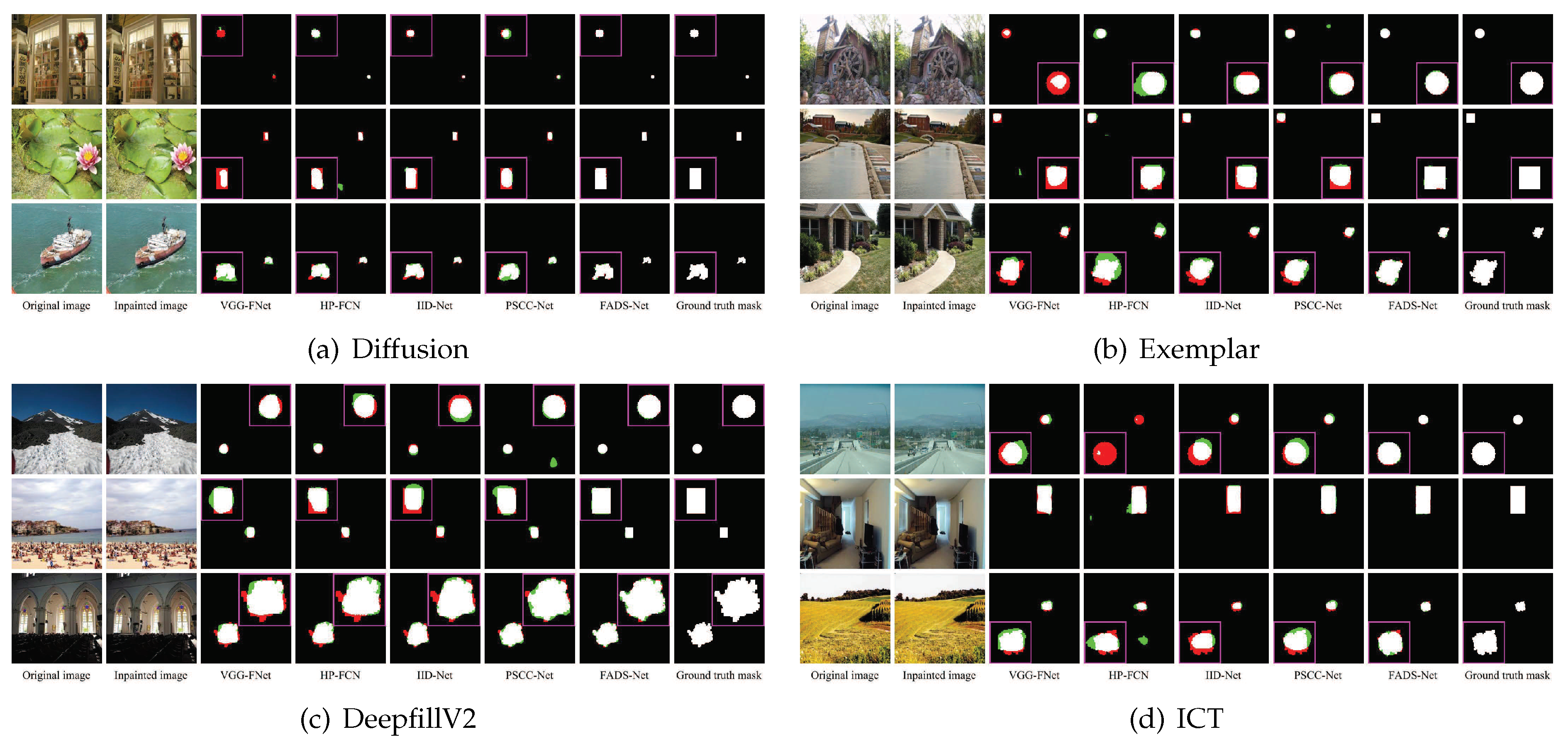
Firstly, we evaluate the forensics performance of FADS-Net by qualitative and quantitative methods on each testing dataset without postprocessing. Figure 7 visually displays the forensic results obtained on several sample images generated by four typical inpainting methods.

Figure 7a,b exhibit the forensic effects for two traditional inpainting methods, i.e., diffusion-based and exemplar-based inpainting [10,62], respectively. Apparently, our method (see the 7th column) achieves quite accurate predictions with little error, while the comparison methods (see columns 3 to 6) yield significant false positive and false negative regions, especially in the 3rd row of Figure 7b. The forensic results illustrate that VGG-FNet [22] (the third column) manifests more false negative errors, while HP-FCN [23] (the fourth column) presents worse false positive performance. For these given sample images, the predictions of IID-Net [26] and PSCC-Net [24] (the fifth and sixth columns) are only slightly better than the previous two methods, and worse than our results.

For two deep learning-based inpainting methods, i.e., ICT [13] and DeepfillV2 [12], the forensic results are shown in Figure 7c,d, respectively. It is noticeable that the performances of VGG-FNet [22], HP-FCN [23], and IID-Net [26] are similar, and there are prediction results with significant false positive or negative errors, e.g., the results of VGG-FNet, HP-FCN, and IID-Net in the third row of Figure 7c and first row of Figure 7d. PSCC-Net [24] reaches a better performance, but it is still inferior to our model.

In principle, the forensic effects of all the tested methods become much worse for the inpainted regions with lower tampering ratios (e.g., the first row of Figure 7a) or uniform regions (e.g., the third row of Figure 7d). Generally, the inpainting effects of small or uniform regions are more realistic, and fewer inpainting traces are left, thus causing difficulties in forensics. In addition, the edges of inpainting regions, especially irregular regions (e.g., the third rows of Figure 7a–d), are more prone to prediction errors. Impressively, our FADS-Net obtains forensic results (in the penultimate columns of Figure 7a–d) best fitting with the ground truth masks (in the last columns of Figure 7a–d) for inpainted regions with different shapes and scales.

Then, the forensic performance is measured by two objective metrics: IoU and F1-score. The average values of IoU and F1-score obtained by the tested methods are summarized in

Table 1. Average IoU (%) and F1 (%) values of forensic results on different forensic datasets with no postprocessing. The best results are marked in bold.

Method	Diffusion			Exemplar			ICT			DeepfillV2
	IoU	F1		IoU	F1		IoU	F1		IoU	F1
VGG-FNet [22]	62.05	68.44		76.64	84.96		69.50	75.97		67.65	76.65
HP-FCN [23]	71.25	76.68		76.28	85.03		78.44	85.81		62.85	72.45
IID-Net [26]	71.01	75.17		88.05	93.18		81.36	87.55		60.92	68.26
PSCC-Net [24]	61.54	67.21		86.15	92.26		85.72	91.84		80.63	88.47
FADS-Net	88.07	91.56		94.67	97.18		91.95	95.61		91.27	95.30

on four testing datasets. The best results are marked in bold.

All compared methods achieve relatively low forensic performance on the forensic dataset for diffusion-based inpainting, mainly due to the image with a smaller inpainting ratio and weak inpainting traces left. For example, PSCC-Net achieves IoU of approximately 61.5% and F1-score of approximately 67.2%, which is close to the performance of VGG-FNet. IID-Net also has a similar performance to HP-FCN, both reaching slightly higher than IoU of 70.0% and F1 score of 75.0%. Surprisingly, FADS-Net presents IoU of approximately 88.07% and F1 score of approximately 91.56%, which is obviously superior to other methods. The performance gain of FADS-Net may be obtained by the design of mining inpainting traces and refining spatial information.

On the forensic dataset for exemplar-based inpainting, each tested method yields larger IoU and F1 than the previous inpainting dataset. For instance, the IoU of PSCC-Net increases from approximately 61.5% to 86.2%. Clearly, the phenomenon indicates that it is easier to locate a larger inpainted region. IID-Net also has a performance close to PSCC-Net and outperforms VGG-FNet and HP-FCN by approximately 10% in IoU and more than 8% in F1 score. Our FADS-Net is approximately 6.7% and 4.0% higher in IoU and F1 score, respectively, than the second-best IID-Net. This is consistent with the qualitative results given previously.

For the ICT dataset, the forensic performance of PSCC-Net presents approximately 85.7% in IoU and 91.8% in F1-score, and ours (91.34% in IoU and 95.27% in F1-score) explicit exceed its performance. Other compared methods reach IoU from 69% to 82%, and F1 score from 75% to 88%. On the DeepfillV2 dataset, except for VGG-FNet and our FADS-Net, the tested methods emerge with significant performance degradation. Similarly, FADS-Net once again exhibits the best performance and has quite a large margin in IoU, approximately 10.6%, compared with the second-best method.

Figure 8a–c respectively show the influence of the inpainted regions with various shapes and scales on the forensics performance. Observing Figure 8a, as the scale of the inpainting region decreases, the forensic performance of all methods decreases dramatically. The effect is the most prominent on the dataset for diffusion-based inpainting, which again confirms the difficulty of forensics for the small inpainted region. In addition, through comparing the results of the diffusion dataset in Figure 8a–c, all the tested methods generally have the lower IoU for irregular masks and the larger one for circular or rectangular masks. This situation also almost obtains on the other three datasets. According to the above analysis, due to the AFRM, dual-stream feature fusion encoders, and attention-based feature fusion, the proposed method provides optimal and stable forensic performance for masks with various shapes and scales.

4.4. Quantitative Evaluation under Typical Attacks

In practice, some postprocessing operations might be performed by forgers after inpainting to hide traces of tampering and evade forensic detection. Thus, we investigate the robustness of the proposed method against JPEG compression and AWGN. These manipulations are considered because they are often employed in many applications.

Specifically, forensics is performed on the distorted images by JPEG compression with QFs of 95, 85, and 75, and AWGN with signal-to-noise ratios (SNRs) of 50 dB, 45 dB, 40 dB, and 35 dB. The average values of IoU and F1-score obtained by the tested methods on the established datasets are reported in

Table 2. Average IoU (%) and F1 score (%) values of different methods on the dataset for diffusion-based inpainting [8] under JPEG compression (QF) and AWGN (SNR) attacks. The best results are marked in bold.

Attack	VGG-FNet [22]			HP-FCN [23]			IID-Net [26]			PSCC-Net [24]			FADS-Net
	IoU	F1		IoU	F1		IoU	F1		IoU	F1		IoU	F1
w/o Dis.	62.05	68.44		71.25	76.68		71.01	75.17		61.54	67.21		88.07	91.56
JPEG 95	60.89	67.11		68.99	74.36		69.93	74.10		60.14	65.75		86.03	89.76
JPEG 85	59.41	65.44		64.48	69.61		67.76	71.94		57.89	63.51		80.13	84.15
JPEG 75	56.93	62.75		58.41	63.28		63.46	67.42		54.37	59.96		73.25	77.22
AWGN 50	61.78	68.13		70.68	76.09		70.82	74.99		61.33	67.00		87.72	91.19
AWGN 45	61.61	67.98		69.77	75.18		70.53	74.69		60.91	66.58		86.41	89.83
AWGN 40	61.15	67.48		68.78	74.21		70.00	74.17		59.93	65.63		85.38	88.86
AWGN 35	60.26	66.46		66.14	71.64		68.58	72.76		58.60	64.30		83.13	86.63

,

Table 3. Average IoU (%) and F1 score (%) values of different methods on the dataset for exemplar-based inpainting [10] under JPEG compression (QF) and AWGN (SNR) attacks. The best results are marked in bold.

Attack	VGG-FNet [22]			HP-FCN [23]			IID-Net [26]			PSCC-Net [24]			FADS-Net
	IoU	F1		IoU	F1		IoU	F1		IoU	F1		IoU	F1
w/o Dis.	76.64	84.96		76.28	85.03		88.05	93.18		86.15	92.26		94.67	97.18
JPEG 95	69.79	78.58		71.62	81.11		85.54	91.48		83.40	90.51		92.91	96.20
JPEG 85	56.66	65.48		50.75	61.08		70.95	78.15		70.86	79.90		86.81	92.13
JPEG 75	49.65	58.26		33.27	42.66		50.23	57.98		47.59	56.57		72.10	79.73
AWGN 50	76.02	84.31		75.20	84.17		87.34	92.54		85.71	91.90		94.54	97.10
AWGN 45	75.28	83.55		74.14	83.29		86.72	91.97		85.15	91.43		94.17	96.81
AWGN 40	74.08	82.38		73.80	82.82		85.99	91.37		84.14	90.61		93.47	96.28
AWGN 35	72.21	80.68		72.39	81.33		84.65	90.32		82.20	88.95		92.45	95.51

,

Table 4. Average IoU (%) and F1 score (%) values of different methods on the ICT [13] dataset under JPEG compression (QF) and AWGN (SNR) attacks. The best results are marked in bold.

Attack	VGG-FNet [22]			HP-FCN [23]			IID-Net [26]			PSCC-Net [24]			FADS-Net
	IoU	F1		IoU	F1		IoU	F1		IoU	F1		IoU	F1
w/o Dis.	69.50	75.97		78.44	85.81		81.36	87.55		85.72	91.84		91.95	95.61
JPEG 95	66.09	72.32		68.70	77.31		74.60	80.73		80.27	87.66		90.93	95.03
JPEG 85	62.71	68.57		55.14	63.49		63.53	69.19		71.59	79.51		83.87	89.08
JPEG 75	59.01	64.77		41.37	49.60		51.91	56.77		61.95	69.97		72.43	78.59
AWGN 50	69.29	75.76		77.57	85.13		81.10	87.32		85.55	91.72		91.72	95.45
AWGN 45	68.68	75.08		75.97	83.92		79.93	86.18		85.09	91.34		91.57	95.40
AWGN 40	67.87	74.27		73.17	81.24		78.29	84.53		83.82	90.22		90.91	94.90
AWGN 35	65.98	72.31		69.64	77.65		74.79	80.92		81.20	87.75		89.66	93.88

and

Table 5. Average IoU (%) and F1 score (%) values of different methods on the DeepfillV2 [12] dataset under JPEG compression (QF) and AWGN (SNR) attacks. The best results are marked in bold.

Attack	VGG-FNet [22]			HP-FCN [23]			IID-Net [26]			PSCC-Net [24]			FADS-Net
	IoU	F1		IoU	F1		IoU	F1		IoU	F1		IoU	F1
w/o Dis.	67.65	76.65		62.85	72.45		60.92	68.26		80.63	88.47		91.27	95.30
JPEG 95	60.19	68.8		54.53	63.72		55.25	62.69		76.15	84.94		90.43	94.81
JPEG 85	53.58	62.22		46.89	56.39		45.75	52.67		61.71	71.02		84.55	90.53
JPEG 75	52.88	61.58		40.91	49.95		41.38	48.06		50.54	58.88		65.42	72.94
AWGN 50	67.44	76.41		60.56	70.43		60.22	67.51		78.81	86.99		90.85	95.00
AWGN 45	66.87	75.94		58.84	68.98		59.00	66.27		78.07	86.34		90.34	94.72
AWGN 40	64.83	73.65		57.18	67.26		56.27	63.52		77.06	85.25		88.48	94.14
AWGN 35	62.42	71.15		54.55	63.99		52.59	59.62		72.96	81.20		87.33	92.38

. Notice that none of these postprocessing operations with the above parameter settings are used to create our training datasets. The best results are marked in bold.

From Table 2, all tested methods experience significant performance degradation as QF or SNR decrease. For instance, FADS-Net receives IoU of 86.03% and F1-score of 89.76% for the case of QF = 0.95, which are slightly lower than those obtained under no attacks, while only approximately IoU of 73% and F1-score of 77% are received under QF = 75. Notice that some forensic networks are relatively insensitive to JPEG compression since they obtain a little lower IoU and F1-score on the images with no distortions, e.g., VGG-FNet [22]. For AWGN with SNR from 50 dB to 35 dB, the IoU and F1-score of FADS-Net are reduced to 92.45% from 94.54% and 95.51% from 97.10%, respectively. The performance degradation is approximately 2%, and the compared methods are subjected to a similar slight performance drop. The above results reveal that all tested methods have more stable robustness against AWGN than JPEG compression. The main reason is that JPEG compression tries to remove the content-unrelated information while guaranteeing the image quality; thus, some inpainting traces are further masked during this process. Similar observations can be made from Table 3, Table 4 and Table 5 on the other three datasets. Impressively, our model outperforms other methods significantly despite different datasets and attack parameters. As an example, FADS-Net outperforms the second-best PSCC-Net [24] by nearly 10.0% in IoU and 8.0% in F1-score under QF = 75 in Table 4. This reveals that our forensic method is more effective for capturing inpainting traces.

4.5. Ablation Analysis

We perform ablation experiments to investigate the effect of two feature extraction streams (RIS and FRS), dense-scale feature fusion module (DFFM), Locality-Sensitive Attention Module (LSAM), and IoU-aware joint loss (IJL) through ablation experiments. For this purpose, we construct the following variants of our full model (FADS-Net).

• RISS-Net: The variant refers to a single-stream encoder network, which takes the original inpainted image as input. Because the encoder is changed to a single-stream structure, the DFFM is removed, but the LSAM module in the decoder is still retained. Moreover, the network training makes use of a hybrid loss that combines CE loss and IoU loss.
• FRSS-Net: The setting of this network is consistent with RIS, except that its single-stream encoder employs FRS.
• DSCF-Net: The network architecture is the same as that of our full model but it discards DFFM and uses simple concatenation to fuse features.
• DSAF-Net: This variant employs the full encoder and loss function of the full model, yet the decoder employs element-wise addition to recover spatial information instead of LSAM.
• FADS-Net (MCL): The network has the same structure as the full model but removes two branch decoders and uses CE loss to supervise the difference between the output of the main decoder and the ground truth label.
• FADS-Net (JCL): CE loss is applied to optimize the results of the main decoder and branch decoder of the full model during training.
• FADS-Net (MHL): The network utilizes a hybrid loss established by combining CE loss and IoU loss to train the full model removing two branch decoders.

All these variants are trained on the DeepfillV2 dataset with the same training options as those of the full model. The average quantitative results are listed in

Table 6. Average IoU (%) and F1 score (%) values of forensic results on the DeepfillV2 [12] dataset for different variants of FADS-Net without and with postprocessing. The best results are marked in bold.

Variant	w/o Dis.			JPEG 75			AWGN 35 dB			Mean
	IoU	F1		IoU	F1		IoU	F1		IoU	F1
RISS-Net	89.07	94.04		56.67	65.33		84.03	90.21		76.59	83.19
FRSS-Net	89.47	94.33		59.22	68.20		84.35	90.55		77.68	84.36
DSCF-Net	90.45	94.86		63.53	72.16		86.24	91.81		80.07	86.28
DSAF-Net	90.75	95.03		61.84	69.39		86.64	91.97		79.74	85.46
FADS-Net (MCL)	89.72	94.43		60.73	68.09		85.87	91.56		78.77	84.69
FADS-Net (JCL)	90.93	95.12		59.94	66.87		87.28	92.30		79.38	84.76
FADS-Net (MHL)	90.27	94.74		61.09	69.44		85.43	91.00		78.93	85.06
FADS-Net	91.27	95.30		65.42	72.94		87.33	92.38		81.34	86.87

, where no extra distortions, JPEG compression with QF = 75, and AWGN with SNR = 35 dB are considered. The best results are marked in bold.

As shown in Table 6, by removing two feature extraction streams, the network with a single-stream encoder only achieves IoU of near 89% and F1 scores of approximately 94% with no distortions averaged on the whole testing dataset, and obtains lower IoU and F1 score under attacks, particularly JPEG compression. The performance is much worse than that of our full model, but is still competitive or superior to that of the former state-of-the-art models for comparison in the considered cases. This shows that the high-resolution structure of encoder and efficient feature extraction module MSDM are beneficial to forensic performance. In addition, FRS has a significant performance improvement over RIS under JPEG compression, which indicates that learning in the frequency domain plays a key role in enhancing the inpainting trace.

The performance is further improved by two variants with dual-stream feature extraction. Although DFFM and LSAM were removed, DSCF-Net and DSAF-Net still exceed two single-stream variants by approximately 2.5% to 3.5% in both average scores of IoU and F1. These results imply that the dual-stream feature fusion can effectively improve the performance of inpainting forensics. By comparing the above two variants with the full model, we may get to know the contribution of DFFM and LSAM. For example, the full model outperforms DSCF-Net by approximately 1.1% in IoU score at SNR = 35 db and produces larger performance margin in the case of DSAF-Net with QF = 75.

Through analyzing the performance of the remaining three variants, the full model has the best performance despite whether or not the tested images undergo some attacks. From the results of the full model and variant FADS-Net (MCL), the use of IoU-aware joint loss increases the performance margin by approximately 2.0% in average IoU and 2.1% in average F1. In particular, the performance of the complete model is approximately 4.5% higher than that of the methods without IAL in the case of QF = 75. Thus, we can confirm that IoU-aware joint loss can drive networks to focus on the inpainted regions more than CEL and ensure that the two-stream feature extraction works effectively.

All the results of the above ablation experiments exhibit that all the components present performance improvement and contribute to the overall performance.

5. Conclusions

In this paper, a novel deep learning method for image inpainting forensics, called FADS-Net, has been presented. In order to locate the tampered regions by inpainting operation, FADS-Net is constructed by following the encoder–decoder network structure. The encoder is a dual-stream network composed of an adaptive frequency recalibration module, two feature extraction sub-networks, and a feature fusion module. The two feature streams can efficiently extract feature maps from the original input and the one recalibrated by this adaptive frequency recalibration module. Then, through the feature fusion module, these extracted features are fully fused to generate more comprehensive and effective feature representations. By introducing the attention mechanism, the decoder can restore more spatial information while improving the feature resolution. Last, we propose an IoU-aware joint loss to guide the training of FADS-Net, where the item of IoU loss takes the forensics performance as the optimization objective, and CE loss can ensure the stability of training and the validity of various parts.

FADS-Net has been extensively tested on various images and several typical inpainting methods and compared with the state-of-the-art forensics methods. Qualitative and quantitative experimental results show that the proposed network can locate the inpainting region more accurately and achieve superior performance in terms of IoU and F1-score. Moreover, our network shows excellent robustness against commonly used post-processing, including JPEG compression and AWGN.

References

1. Alipour, N.; Behrad, A. Semantic segmentation of JPEG blocks using a deep CNN for non-aligned JPEG forgery detection and localization. Multimedia Tools Appl. 2020, 79, 8249–8265. [Google Scholar] [CrossRef]
2. Bakas, J.; Ramachandra, S.; Naskar, R. Double and triple compression-based forgery detection in JPEG images using deep convolutional neural network. J. Electron. Imaging 2020, 29, 023006. [Google Scholar] [CrossRef]
3. Zhang, J.; Liao, Y.; Zhu, X.; Wang, H.; Ding, J. A deep learning approach in the discrete cosine transform domain to median filtering forensics. IEEE Signal Process. Lett. 2020, 27, 276–280. [Google Scholar] [CrossRef]
4. Abhishek; Jindal, N. Copy move and splicing forgery detection using deep convolution neural network, and semantic segmentation. Multimedia Tools Appl. 2021, 80, 3571–3599. [Google Scholar] [CrossRef]
5. Liu, B.; Pun, C.M. Exposing splicing forgery in realistic scenes using deep fusion network. Inf. Sci. 2020, 526, 133–150. [Google Scholar] [CrossRef]
6. Mayer, O.; Stamm, M.C. Forensic similarity for digital images. IEEE Trans. Inf. Forensics Secur. 2020, 15, 1331–1346. [Google Scholar] [CrossRef] [Green Version]
7. Mayer, O.; Bayar, B.; Stamm, M.C. Learning unified deep-features for multiple forensic tasks. In Proceedings of the 6th ACM Workshop on Information Hiding and Multimedia Security, Innsbruck, Austria, 20–22 June 2018; pp. 79–84. [Google Scholar]
8. Bertalmio, M.; Sapiro, G.; Caselles, V.; Ballester, C. Image inpainting. In Proceedings of the 27th Internationl Conference on Computer Graphics and Interactive Techniques Conference, New Orleans, LA, USA, 23–28 July 2000; pp. 417–424. [Google Scholar]
9. Oliveira, M.M.; Bowen, B.; McKenna, R.; Chang, Y.S. Fast digital image inpainting. In Proceedings of the International Conference on Visualization, Imaging and Image Processing (VIIP 2001), Marbella, Spain, 3–5 September 2001; pp. 106–107. [Google Scholar]
10. Criminisi, A.; Perez, P.; Toyama, K. Region filling and object removal by exemplar-based image inpainting. IEEE Trans. Image Process. 2004, 13, 1200–1212. [Google Scholar] [CrossRef]
11. Ružić, T.; Pižurica, A. Context-aware patch-Based image inpainting using Markov random field modeling. IEEE Trans. Image Process. 2015, 24, 444–456. [Google Scholar] [CrossRef]
12. Yu, J.; Lin, Z.; Yang, J.; Shen, X.; Lu, X.; Huang, T. Free-form image inpainting with gated convolution. In Proceedings of the IEEE/CVF International Conference on Computer Vision (ICCV), Seoul, Republic of Korea, 27 October–2 November 2019; pp. 4470–4479. [Google Scholar]
13. Wan, Z.; Zhang, J.; Chen, D.; Liao, J. High-fidelity pluralistic image mcopletion with transformers. In Proceedings of the IEEE/CVF International Conference on Computer Vision (ICCV), Virtually, 11–17 October 2021; pp. 4672–4681. [Google Scholar]
14. Chang, I.; Yu, J.C.; Chang, C.C. A forgery detection algorithm for exemplar-based inpainting images using multi-region relation. Image Vis. Comput. 2013, 31, 57–71. [Google Scholar] [CrossRef]
15. Liang, Z.; Yang, G.; Ding, X.; Li, L. An efficient forgery detection algorithm for object removal by exemplar-based image inpainting. J. Vis. Commun. Image R. 2015, 30, 75–85. [Google Scholar] [CrossRef]
16. Li, H.; Luo, W.; Huang, J. Localization of diffusion-based inpainting in digital images. IEEE Trans. Inf. Forensics Secur. 2017, 12, 3050–3064. [Google Scholar] [CrossRef]
17. Zhang, Y.; Liu, T.; Cattani, C.; Cui, Q.; Liu, S. Diffusion-based image inpainting forensics via weighted least squares filtering enhancement. Multimedia Tools Appl. 2021, 80, 30725–30739. [Google Scholar] [CrossRef]
18. Ronneberger, O.; Fischer, P.; Brox, T. U-net: Convolutional networks for biomedical image segmentation. In Proceedings of the Medical Image Computing and Computer-Assisted Intervention–MICCAI 2015, Munich, Germany, 5–9 October 2015; pp. 234–241. [Google Scholar]
19. Zhu, X.; Li, S.; Gan, Y.; Zhang, Y.; Sun, B. Multi-stream fusion network with generalized smooth L1 loss for single image dehazing. IEEE Trans. Image Process. 2021, 30, 7620–7635. [Google Scholar] [CrossRef]
20. Pang, J.; Chen, K.; Shi, J.; Feng, H.; Ouyang, W.; Lin, D. Libra R-CNN: Towards balanced learning for object detection. In Proceedings of the IEEE/CVF Conference on Computer Vision and Pattern Recognition (CVPR), Long Beach, CA, USA, 16–20 June 2019; pp. 821–830. [Google Scholar]
21. Rafi, A.M.; Tonmoy, T.I.; Kamal, U.; Wu, Q.M.J.; Hasan, M.K. RemNet: Remnant convolutional neural network for camera model identification. Neural Comput. Appl. 2021, 33, 3655–3670. [Google Scholar] [CrossRef]
22. Zhu, X.; Qian, Y.; Zhao, X.; Sun, B.; Sun, Y. A deep learning approach to patch-based image inpainting forensics. Signal Process. Image Commun. 2018, 67, 90–99. [Google Scholar] [CrossRef]
23. Li, H.; Huang, J. Localization of deep inpainting using high-pass fully convolutional network. In Proceedings of the IEEE/CVF International Conference on Computer Vision (ICCV), Seoul, Republic of Korea, 27 October–2 November 2019; pp. 8301–8310. [Google Scholar]
24. Liu, X.; Liu, Y.; Chen, J.; Liu, X. PSCC-Net: Progressive Spatio-Channel Correlation Network for Image Manipulation Detection and Localization. IEEE Trans. Circuits Syst. 2022, 32, 7505–7517. [Google Scholar] [CrossRef]
25. Bayar, B.; Stamm, M.C. Constrained convolutional neural networks: A new approach towards general purpose image manipulation detection. IEEE Trans. Inf. Forensics Secur. 2018, 13, 2691–2706. [Google Scholar] [CrossRef]
26. Wu, H.; Zhou, J. IID-Net: Image inpainting detection network via neural architecture search and attention. IEEE Trans. Circuits Syst. Video Technol. 2022, 32, 1172–1185. [Google Scholar] [CrossRef]
27. Chen, L.C.; Papandreou, G.; Kokkinos, I.; Murphy, K.; Yuille, A.L. DeepLab: Semantic image segmentation with deep convolutional nets, atrous convolution, and fully connected CRFs. IEEE Trans. Pattern Anal. Mach. Intell. 2018, 40, 834–848. [Google Scholar] [CrossRef] [PubMed] [Green Version]
28. Badrinarayanan, V.; Kendall, A.; Cipolla, R. Segnet: A deep convolutional encoder-decoder architecture for image segmentation. IEEE Trans. Pattern Anal. Mach. Intell. 2017, 39, 2481–2495. [Google Scholar] [CrossRef] [PubMed]
29. Dumoulin, V.; Visin, F. A guide to convolution arithmetic for deep learning. arXiv 2016, arXiv:1603.07285. [Google Scholar]
30. Long, J.; Shelhamer, E.; Darrell, T. Fully convolutional networks for semantic segmentation. In Proceedings of the IEEE Conference on Computer Vision and Pattern Recognition (CVPR), Boston, MA, USA, 7–12 June 2015; pp. 3431–3440. [Google Scholar]
31. Wang, F.; Jiang, M.; Qian, C.; Yang, S.; Li, C.; Zhang, H.; Wang, X.; Tang, X. Residual attention network for image classification. In Proceedings of the IEEE Conference on Computer Vision and Pattern Recognition (CVPR), Honolulu, HI, USA, 21–26 July 2017; pp. 3156–3164. [Google Scholar]
32. Wu, Q.; Sun, S.; Zhu, W.; Li, G.H.; Tu, D. Detection of digital doctoring in exemplar-based inpainted images. In Proceedings of the 2008 International Conference on Machine Learning and Cybernetics, Kunming, China, 12–15 July 2008; Volume 3, pp. 1222–1226. [Google Scholar]
33. Das, S.; Shreyas, G.D.; Devan, L.D. Blind detection method for video inpainting forgery. Int. J. Comput. Appl. 2012, 60, 33–37. [Google Scholar] [CrossRef]
34. Bacchuwar, K.S.; Ramakrishnan, K.R. A jump patch-block match algorithm for multiple forgery detection. In Proceedings of the 2013 International Mutli-Conference on Automation, Computing, Communication, Control and Compressed Sensing (iMac4s), Kottayam, India, 22–23 March 2013; pp. 723–728. [Google Scholar]
35. Trung, D.T.; Beghdadi, A.; Larabi, M.C. Blind inpainting forgery detection. In Proceedings of the 2014 IEEE Global Conference on Signal and Information Processing (GlobalSIP), Atlanta, GA, USA, 3–5 December 2014; pp. 1019–1023. [Google Scholar]
36. Zhao, Y.Q.; Liao, M.; Shih, F.Y.; Shi, Y.Q. Tampered region detection of inpainting JPEG images. Optik 2013, 124, 2487–2492. [Google Scholar] [CrossRef]
37. Liu, Q.; Zhou, B.; Sung, A.H.; Qiao, M. Exposing inpainting forgery in JPEG images under recompression attacks. In Proceedings of the 2016 15th IEEE International Conference on Machine Learning and Applications (ICMLA), Anaheim, CA, USA, 18–20 December 2016; pp. 164–169. [Google Scholar]
38. Zhang, D.; Liang, Z.; Yang, G.; Li, Q.; Li, L.; Sun, X. A robust forgery detection algorithm for object removal by exemplar-based image inpainting. Multimedia Tools Appl. 2018, 77, 11823–11842. [Google Scholar] [CrossRef]
39. Xu, Z.; Sun, J. Image inpainting by patch propagation using patch sparsity. IEEE Trans. Image Process. 2010, 19, 1153–1165. [Google Scholar]
40. Li, Z.; He, H.; Tai, H.M.; Yin, Z.; Chen, F. Color-direction patch-sparsity-based image inpainting using multidirection features. IEEE Trans. Image Process. 2014, 24, 1138–1152. [Google Scholar] [CrossRef]
41. Jin, X.; Su, Y.; Zou, L.; Wang, Y.; Jing, P.; Wang, Z.J. Sparsity-based image inpainting detection via canonical correlation analysis with low-rank constraints. IEEE Access 2018, 6, 49967–49978. [Google Scholar] [CrossRef]
42. Zhu, X.; Qian, Y.; Sun, B.; Ren, C.; Sun, Y.; Yao, S. Image inpainting forensics algorithm based on deep neural network. Acta Opt. Sin. 2018, 38, 1110005-1–1110005-9. [Google Scholar]
43. Lu, M.; Liu, S. A detection approach using LSTM-CNN for object removal caused by exemplar-based image inpainting. Electronics 2020, 9, 858. [Google Scholar] [CrossRef]
44. Wang, X.; Wang, H.; Niu, S. An intelligent forensics approach for detecting patch-based image inpainting. Math. Probl. Eng. 2020, 2020, 8892989. [Google Scholar] [CrossRef]
45. Bender, G.; Kindermans, P.J.; Zoph, B.; Vasudevan, V.; Le, Q. Understanding and simplifying one-shot architecture search. In Proceedings of the 35th International Conference on Machine Learning, Stockholm, Sweden, 10–15 July 2018; Volume 80, pp. 550–559. [Google Scholar]
46. Wang, J.; Sun, K.; Cheng, T.; Jiang, B.; Deng, C.; Zhao, Y.; Liu, D.; Mu, Y.; Tan, M.; Wang, X.; et al. Deep high-resolution representation learning for visual recognition. IEEE Trans. Pattern Anal. Mach. Intell. 2021, 43, 3349–3364. [Google Scholar] [CrossRef] [PubMed] [Green Version]
47. Qian, Y.; Yin, G.; Sheng, L.; Chen, Z.; Shao, J. Thinking in frequency: Face forgery detection by mining frequency-aware clues. In Proceedings of the 16th European Conference, Glasgow, UK, 23–28 August 2020; pp. 86–103. [Google Scholar]
48. Xu, K.; Qin, M.; Sun, F.; Wang, Y.; Chen, Y.K.; Ren, F. Learning in the frequency domain. In Proceedings of the IEEE/CVF Conference on Computer Vision and Pattern Recognition (CVPR), Virtually, 14–19 June 2020; pp. 1740–1749. [Google Scholar]
49. Hu, J.; Shen, L.; Sun, G. Squeeze-and-excitation networks. In Proceedings of the IEEE Conference on Computer Vision and Pattern Recognition (CVPR), Salt Lake City, UT, USA, 18–22 June 2018; pp. 7132–7141. [Google Scholar]
50. Chen, L.C.; Papandreou, G.; Schroff, F.; Adam, H. Rethinking atrous convolution for semantic image segmentation. arXiv 2017, arXiv:1706.05587. [Google Scholar]
51. Huang, G.; Liu, Z.; Maaten, L.V.D.; Weinberger, K.Q. Densely connected convolutional networks. In Proceedings of the IEEE Conference on Computer Vision and Pattern Recognition (CVPR), Honolulu, HI, USA, 21–26 July 2017; pp. 4700–4708. [Google Scholar]
52. Yang, M.; Yu, K.; Zhang, C.; Li, Z.; Yang, K. DenseASPP for semantic segmentation in street scenes. In Proceedings of the IEEE Conference on Computer Vision and Pattern Recognition (CVPR), Salt Lake City, UT, USA, 18–22 June 2018; pp. 3684–3692. [Google Scholar]
53. Wang, Z.; Chen, J.; Hoi, S.C.H. Deep learning for image super-resolution: A survey. IEEE Trans. Pattern Anal. Mach. Intell. 2021, 43, 3365–3387. [Google Scholar] [CrossRef] [Green Version]
54. Itti, L.; Koch, C.; Niebur, E. A model of saliency-based visual attention for rapid scene analysis. IEEE Trans. Pattern Anal. Mach. Intell. 1998, 20, 1254–1259. [Google Scholar] [CrossRef] [Green Version]
55. Rensink, R. The dynamic representation of scenes. Vis. Cognit. 2000, 7, 17–42. [Google Scholar] [CrossRef]
56. Corbetta, M.; Shulman, G.L. Control of goal-directed and stimulus-driven attention in the brain. IEEE Trans. Pattern Anal. Mach. Intell. 2002, 3, 201–215. [Google Scholar] [CrossRef]
57. Fu, J.; Liu, J.; Tian, H.; Li, Y.; Bao, Y.; Fang, Z.; Lu, H. Dual attention network for scene segmentation. In Proceedings of the IEEE/CVF Conference on Computer Vision and Pattern Recognition (CVPR), Long Beach, CA, USA, 16–20 June 2019; pp. 3146–3154. [Google Scholar]
58. Tian, Y.; Hu, W.; Jiang, H.; Wu, J. Densely connected attentional pyramid residual network for human pose estimation. Neurocomputing 2019, 347, 13–23. [Google Scholar] [CrossRef]
59. Woo, S.; Park, J.; Lee, J.Y.; Kweon, I.S. CBAM: Convolutional block attention module. In Proceedings of the European Conference on Computer Vision (ECCV), Munich, Germany, 8–14 September 2018; pp. 3–19. [Google Scholar]
60. Li, W.; Zhu, X.; Gong, S. Harmonious Attention Network for Person Re-Identification. In Proceedings of the IEEE Conference on Computer Vision and Pattern Recognition (CVPR), Salt Lake City, UT, USA, 18–22 June 2018; pp. 2285–2294. [Google Scholar]
61. Zhou, B.; Lapedriza, A.; Xiao, J.; Torralba, A.; Oliva, A. Learning deep features for scene recognition using places database. In Advances in Neural Information Processing Systems; NeurIPS: San Diego, CA, USA, 2014; Volume 27, pp. 487–495. [Google Scholar]
62. G’MIC. GREYC’s Magic for Image Computing. 2021. Available online: http://gmic.eu (accessed on 25 February 2023).
Figure 1. An illustrative example of image tampering by image inpainting: the real image (left), the inpainted image (middle), and the utilized mask (right).
Mathematics 11 02593 g001
Figure 2. The architecture of the proposed frequency attention-based dual-stream inpainting forensics network (FADS-Net). FADS-Net has the same structure as encoder–decoder networks. The two feature extraction streams extract features from the input image, and two features are fused using a dense feature fusion module (DFFM) to generate the final feature response of the encoder. Then through the attention-based decoder, the fed features are progressively refined and the spatial resolution is restored for the final dense predictions.
Mathematics 11 02593 g002
Figure 3. The architecture of the adaptive frequency recalibration module.
Mathematics 11 02593 g003
Figure 4. The architecture of dense-scale feature fusion module (DFFM). An example of receptive field (RF) formed in the MSDM DF is shown on the right side of the figure.
Mathematics 11 02593 g004
Figure 5. The structure of the locality-sensitive attention module (LSAM). LSAM is composed of channel and spatial attention modules, where the upper network branch depicts the structure of channel attention module and the bottom network branch depicts the structure of spatial attention module.
Mathematics 11 02593 g005
Figure 6. Examples for images in datasets. From left to right: original images, images with the missing regions (marked in green), inpainted images, and ground truth masks.
Mathematics 11 02593 g006
Figure 7. Qualitative comparisons of different forensic methods on the images tampered by (a) diffusion-based inpainting [62], (b) exemplar-based inpainting [10], (c) DeepfillV2 [12], and (d) ICT [13]. The original uninpainted images, inpainted images, forensic results obtained by the methods in [22,23,24,26] and our method, as well as ground truth masks are shown in columns 1 to 8, where the pixels in white, black, green, and red indicate true positive, true negative, false positive, and false negative, respectively. For better visual comparison, the zoom-in versions of the predicted tampering regions marked by the pink rectangles are shown in a corner.
Mathematics 11 02593 g007
Figure 8. Comparison of different forensic methods for inpainted regions (IRs) with different scales on Diffusion, Exemplar, ICT, and DeepfillV2 datasets, respectively.
Mathematics 11 02593 g008