1. Introduction
The increasing volume and complexity of real-life data structures push researchers to shift from conventional machine learning to deep learning.
Conventional machine-learning techniques have limited ability to process data in their raw form: hence, demanding careful engineering and substantial domain expertise to transform the raw data into a feature vector that can serve as a proper input to the algorithm.
Deep learning methods allow replacing hand-engineered features with multilayer networks trained to discover the structures in data. Therefore, a machine learning algorithm can take raw data to automatically discover hidden structures needed for detection or classification [
1].
The brightest example of deep learning algorithms includes convolutional neural networks (CNNs) used to process images or videos, where the raw data comes in the form of ordered 2-D or 1-D arrays of pixels. Each layer of a CNN performs convolutional operations on the image followed by a non-linear activation. The keys of CNNs are local connection, shared weights, and the use of multiple layers [
2].
The main limitation of the CNNs is that they can only operate on regular Euclidean data, such as images (2-D grids) and texts (1-D sequences). At the same time, much real-life data comes in the non-Euclidean form, e.g., graph-structured data. The specific examples include but are not limited to social networks, DNA and RNA sequences, transportation, and brain neural networks. Therefore, solving classification, clusterization, and other problems on graphs becomes of great interest and importance [
3].
In recent years, graph neural networks (GNN) have attracted attention from the machine-learning community. Areas dealing with graph-structured data, such as social networks, molecular structures, and recommendation systems, have undergone significant advancements through the application of GNNs [
4,
5]. There is also interest in applying GNNs to the analysis of functional brain networks, e.g., to classify patients with major depressive disorder and healthy subjects [
6].
GNN enables learning from non-Euclidean data. The absence of a fixed and consistent metric space in such data presents a challenge when applying traditional algorithms that rely on fixed geometries. By leveraging the underlying graph structure, GNNs can effectively capture the complex relationships between nodes and edges in the data and learn to make predictions based on that structure [
7].
The real-life graph data fall into two broad categories: spatially-invariant and spatially-variant graphs. In a spatially-invariant graph, the structure of links between the nodes does not depend on their position in space. A network of social interactions is an example. In a spatially-variant graph, the location of the nodes matters and provides additional information about the graph’s properties. Examples include molecular structures, brain networks, etc. There is a limited understanding of how the performance of GNNs differs between these two classes of graphs and how we can leverage information about the spatial structure to improve the performance of machine learning models.
We can represent a graph with an
adjacency matrix where
m reflects the number of nodes. Each element
of this matrix defines the link between the
i-th and
j-th nodes. In the spatially invariant graph, if you shuffle its edge list or the columns of its adjacency matrix, it is still the same graph (See
Figure 1a).
Figure 1 shows the explanatory case of a small graph consisting of the five nodes (A, B, C, D, E) and four links (A-E, A-C, A-B, B-D). The different panels illustrate the cases of the spatially-invariant (a) and the spatially-variant (b) graphs. The figure also presents their adjacency matrices. On the left, the matrix has columns and rows ordered in alphabetical node order: on the row for node A (first row), we can read that it is connected to E and C. On the right-hand side, the same graph is shown with the different locations of the nodes. On the right, the adjacency matrix is shuffled (the columns are no longer sorted alphabetically). So in the case of the spatially-invariant graphs (a), two matrices give a valid representation of the graph (A is still connected to E and C). For the spatially-variant graphs (b), a shuffled adjacency matrix cannot suffer as a valid representation.
We suggest that an adjacency matrix provides the Euclidean form for a spatially-variant graph but becomes invariant to the permutation of nodes’ indexes in a spatially-invariant graph. Thus, we hypothesize that CNN may outperform GNN when working with spatially-variant graphs while GNN will perform better on the spatially-invariant graphs.
To test this hypothesis, we propose a simple algorithm to generate graphs with predefined spatial structures and connectivity patterns (a sub-structure of the links that the machine learning algorithm should learn). We trained and tested CNN and GNN in two cases. First, the graphs in the training and test sets had the same connectivity pattern (structure of the links between nodes) and spatial structure (location of nodes). Second, graphs in the training and test sets had the same connectivity pattern but different spatial structures.
Our results confirmed the existence of spatial structure in the graph enables using CNN, which may even outperform GNN in some cases. The main contribution of our results is that having prior knowledge about the spatial structure in real-life datasets enables the selection of the most appropriate machine learning algorithm to achieve optimal performance.
2. Materials and Methods
2.1. Graph Generation Algorithm
Here we tested the accuracy of the deep learning algorithms in the classification task performed on the graph-structured data. Therefore, we were required to create two classes of graphs that differed in their connectivity pattern. For simplicity, we defined negative class as fully-connected graphs, where the links’ weights were sampled from the half-normal distribution . In the second positive class, we generated graphs containing a predefined segregated connectivity pattern. We divided all graph nodes into the equal regions (each included nodes, and increased the link’s weight inside 6 regions (we called them active regions through the text). The link’s weights for the active regions were sampled from the normal distribution , where varied from 0 to 7 with the step .
The value of
n is a step number that signifies the distance between
and
(
Figure 2). At
(
Figure 2a) the distributions are the same, meaning that links’ weights were sampled from the same distribution in the entire graph. This results in the same structure across both classes. At
,
(dashed line in
Figure 2b), meaning that the nodes in the active regions get obtain stronger link weights. Further increase of
n results in the strengthening difference in the link weights between the active regions and the rest of the graph (
Figure 2c,d).
To summarize, all graphs have nodes with pre-defined regions, 50% of which are active, and n varies in the range of , determining how distinguished the link weight in active regions from the links in the rest of a graph is.
It should be noted that the algorithm is non-deterministic. Given the same input parameters (, , ), every outcome is different due to sampling. It allowed us to generate graphs that exhibit structural similarities but differ in terms of edge weights.
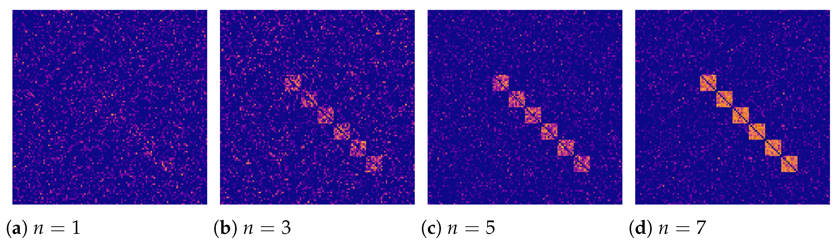
Examining the adjacency matrices, one can see that the graphs in the positive class have a certain pattern on the adjacency matrix (compare
Figure 3 and
Figure 4), which becomes more pronounced with the growing
n. This pattern has a diagonal structure and depends on the ordered number of active regions. When activating the odd regions, this pattern takes the form of an alternating sequence of squares.
2.2. Datasets
This section provides a description of both datasets: spatially-variant and spatially-invariant. It should be noted that training and test tests of positive class within each dataset were different, while negative class was always the same.
2.2.1. Negative Class in Both Datasets
To test if the deep learning algorithms may handle spatially-invariant graphs, we created two datasets. Each dataset has a positive and a negative class. Recalling
Section 2.1, the graphs of negative class are generated with parameter
. By design, such the graphs do not have regions. The weights for nodes’ connections are sampled from the half-normal distribution
.
Figure 3 shows the typical adjacency matrices for the negative class. Panels (a-d) correspond to the different values of
n defining the difference in the link weight between the active regions and the rest of the graph. Since in the negative class, we sampled the link weights from a single distribution for all regions, adjacency matrices demonstrate the homogeneous distribution of the weights that barely depends on
n.
2.2.2. Positive Class in the Spatially-Variant Dataset
The first dataset reflected the case of the spatially-variant graph. The graphs in the training and test sets had the same connectivity pattern (structure of the links between nodes) and spatial structure (location of nodes). To generate the same connectivity pattern, we keep the same number of active regions across the sets. To generate the same spatial structure, we make the same regions active in the training and test sets. To reduce overfitting, we make the structure of the training and test graphs differ from each other. We achieved it by shifting the spatial pattern along the horizontal and vertical dimensions. Specifically, we set the odd regions (1, 3, 5, 7, 9, and 11) active in the training set (
Figure 4), and the even regions (2, 4, 6, 8, 10, and 12) – in the test set (
Figure 5).
2.2.3. Positive Class in the Spatially-Invariant Dataset
The second dataset reflected the case of the spatially-invariant graph. The graphs in the training and test sets had the same connectivity pattern but different spatial structures. To generate the same connectivity pattern, we keep the same number of active regions across the sets. To generate a distinct spatial structure, we make the different regions active in the training and test sets. The training set, depicted in
Figure 6, comprised active regions 1–4 and 11, 12, while active regions 5–10 were incorporated in the test set, as shown in
Figure 7.
Figure 8 summarizes the spatially-invariant and spatially-variant datasets on which both GNN and CNN are trained and tested. It should be noted that the examples are shown for
to highlight the active regions, while we formed similar datasets for various
n.
The training set for both datasets includes 256 samples for each class, and the validation and test sets contain 32 samples per class. It’s important to note that each dataset is balanced and the use of weight sampling ensures that every graph is unique.
2.3. Graph Metrics
Researchers use clustering [
8,
9,
10] and modularity [
11,
12,
13] to measure network segregation. The main difference between the two is that the former does not take regional information (the region a node belongs to) into account, while the latter does.
For unweighted graphs, node
u’s clustering depends on the number of triangles passing through the node,
, and the degree of the node,
:
However, in our case, the graphs are weighted, so we used the formula provided by networkx library and taken from Onnela et al. [
9]. It uses the geometric average of the subgraph formed by nodes
u,
w, and
u:
where
is the weight of connection between
u and
v,
is the maximum weight in the network.
The formula for modularity is more complicated due to taking regional information into account. The metric quantifies the degree to which a network is split into densely connected regions. To calculate modularity, we used bct library.
where
is the weight of connection between nodes
i and
j,
is the degree of node
i,
I is the sum of all weights in the network; it is a normalizing constant, and
Global clustering and modularity of a graph is the average of its nodes’ corresponding metric values. Weighted clustering and modularity measure segregation differently, and further sections depict the difference.
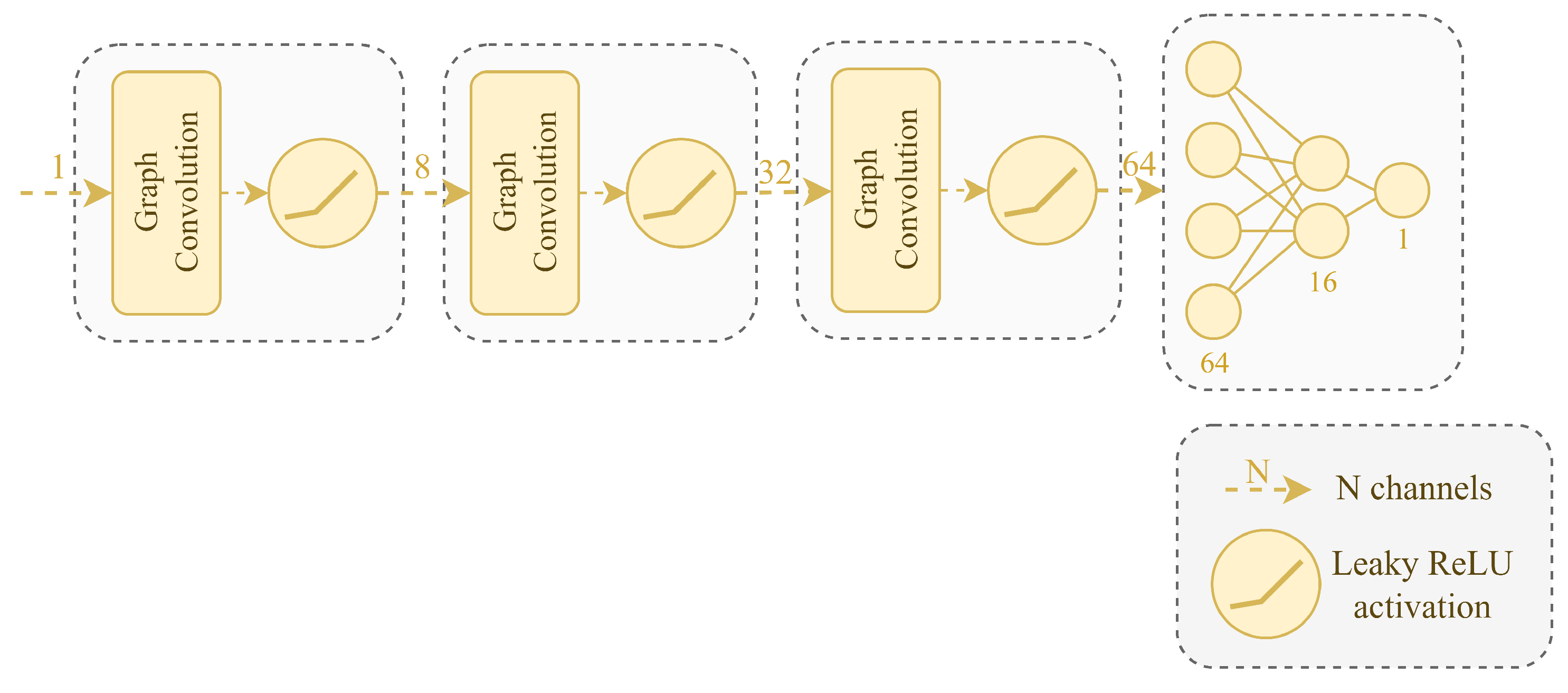
2.4. Graph Neural Network
GNN consists of graph convolutional layers defined by Kipf et al. [
14], Leaky ReLU as activation, dropout layers, and linear layers in the end to obtain output.
Figure 9 shows the architecture (dropout layers are not shown). Overall, the model has 3473 trainable parameters.
To train the model, we used an Adam optimizer with a learning rate of 0.002, weight decay equals zero. To calculate loss, we used Binary Cross Entropy with logits that combines sigmoid activation and Binary Cross Entry loss.
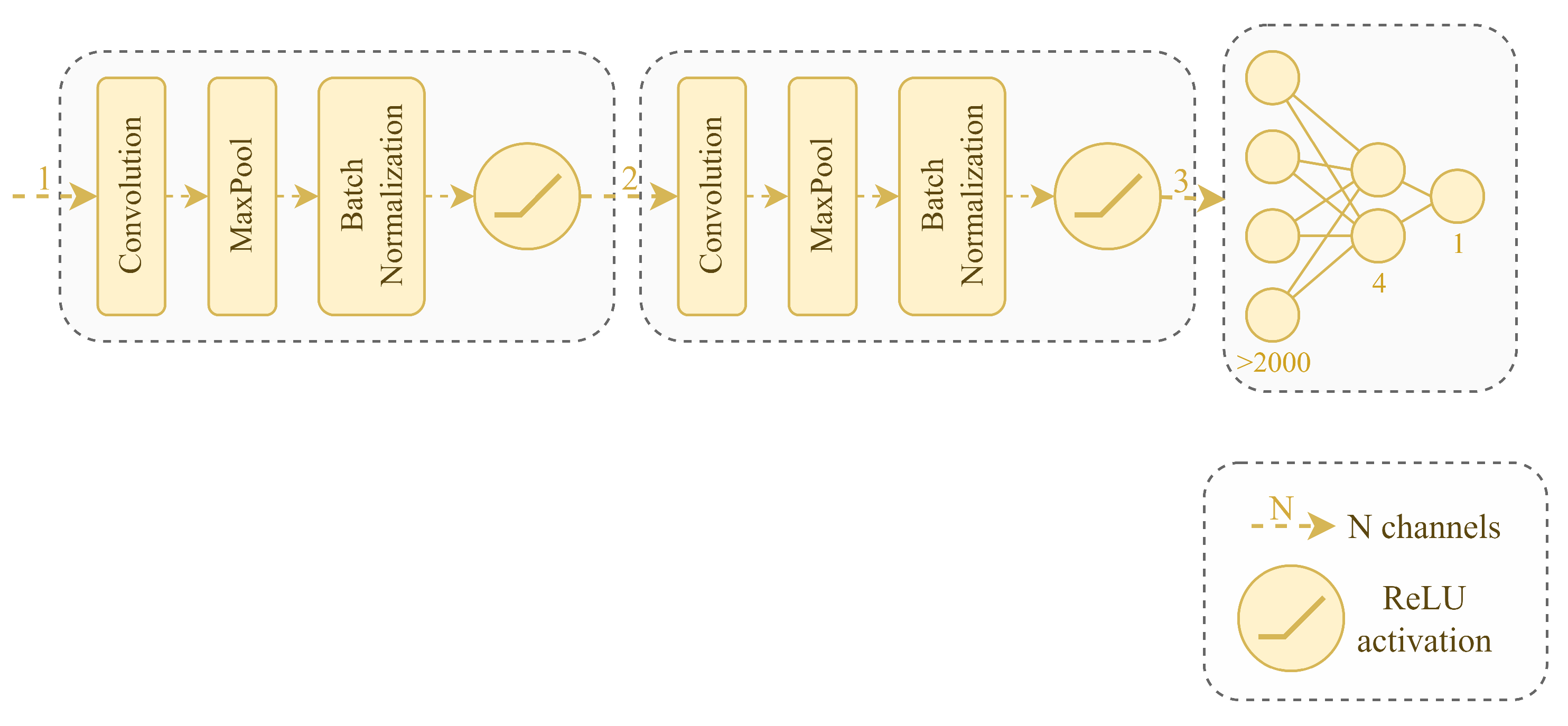
2.5. Convolutional Neural Network
CNN consists of graph convolutional layers, pooling layers, batch normalization, ReLU as activation, dropout layers, and linear layers in the end to obtain output.
Figure 10 shows the architecture (dropout layers are not shown). Overall, the model has 9084 trainable parameters.
A graph is a 1-D image, e.g., gray-scaled because the pixel at index is a number corresponding to the edge’s weight .
To train the model, we used an Adam optimizer with a learning rate of 0.001 and weight decay of 0.0005. To calculate loss, we used binary cross entropy with logits.
We used adjacency matrix representation to turn a graph into an image. This way, our CNN took a batch of 1-D images as input.
2.6. Performance Evaluation
CNN- and GNN-specific parameters were described in the sections above. However, the models have maximum of 100 epochs per training set with early stopping monitoring validation loss. In this case it means that if the model’s loss stopped decreasing for 3 epochs, the training stops. Both models’ hyper-parameters (e.g., learning rate and weight decay) were set through Ray Tune library with grid searcher based on Bayesian Optimization (BayesOptSearch). We ran an optimization algorithm in the following parameter space:
Number of convolutional modules (choice: [1, 2 (CNN), 3 (GNN), 4]);
Learning rate (choice: [0.0001, 0.001 (CNN), 0.002 (GNN), 0.005, 0.01]);
Weight decay (choice: [0 (GNN), 0.00001, 0.0005 (CNN), 0.001]).
The tuner was set to monitor validation loss, meaning that how fast the loss decreases is a crucial factor to a chosen set of hyperparameters. The tuner was run on datasets for n = [1, 4, 7], and we chose the hyperparameters that proved most optimal more often.
For both models, we used a validation set to fine-tune the model and then tested it on the test sets. Accuracy, recall and specificity were calculated as an average across batches of the training and test sets.
3. Results
First, we analyzed how the graph properties change with the varying share of the active regions and the weights inside these regions. We used clustering and modularity coefficients (refer to Methods) to quantify the graph properties.
Figure 11 presents the results. The modularity growth follows the step number
n. With each step, the weights inside active regions further exceed the ones in the rest of the graph (as defined by an algorithm of the dataset generation). Thus, the stronger connection inside the active regions causes higher modularity. The more regions that are active, the higher the graph’ modularity. The clustering coefficient barely responds to the changing weight within active regions. It remains unchanged with an increase in the number of active regions, as depicted in
Figure 11.
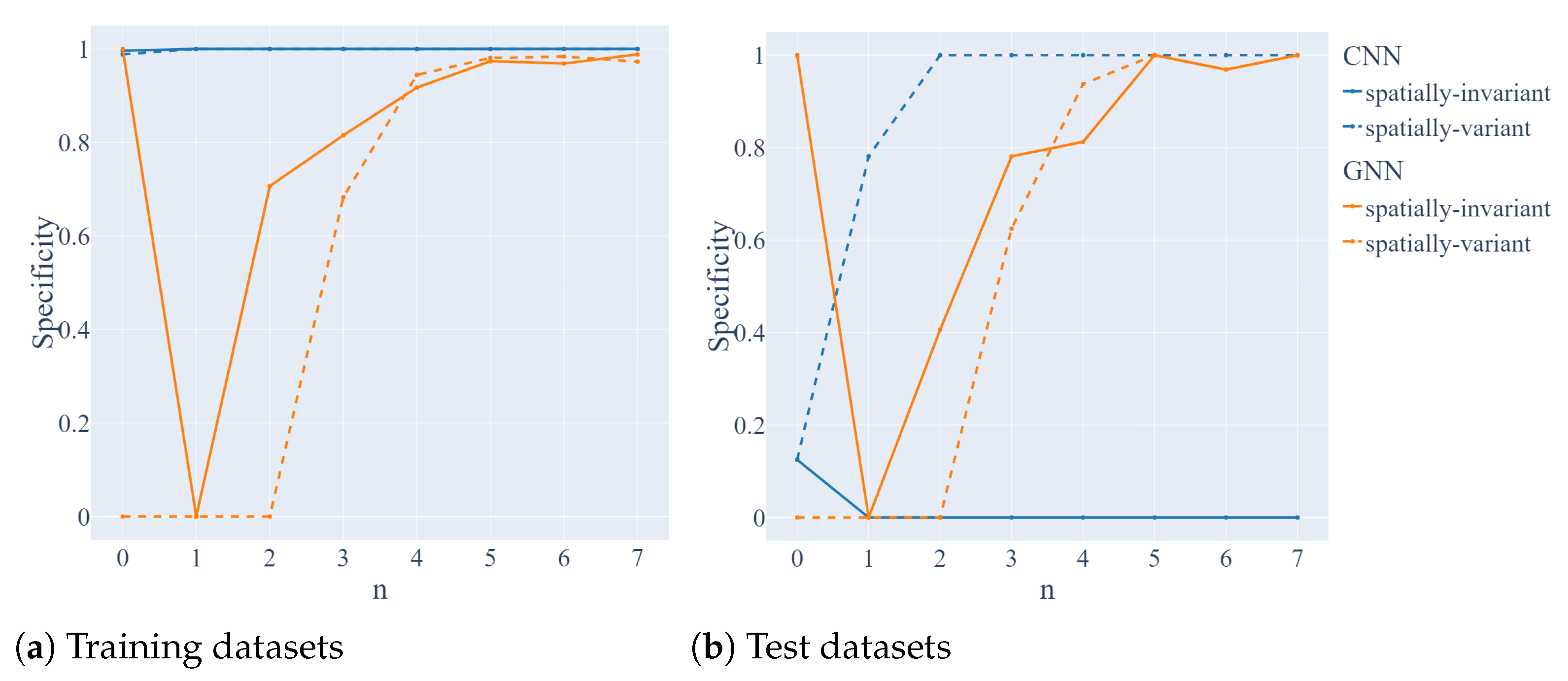
Then, we tested the performance of the GNN and CNN in the graph classification task for different weights within the active regions.
Figure 12 provides complete GNN’s and CNN’s performance information. The step identifies to what extent the weights within the active regions c Panels (a) and (b) correspond to the training and test sets. We considered two graph types: spatially-variant and spatially-invariant. Recall that the spatially-variant type represents the case when the adjacency matrices have a similar structure among the training and test set but shifted along the horizontal and vertical dimensions as depicted in
Figure 4 and
Figure 5. On the contrary, spatially-invariant corresponds to the case when the spatial structure on the adjacency matrices differs between the training and test sets. Unlike the spatially-variant case, the spatial structure of the adjacency matrices in the test set can not be obtained from the training set by shifting along vertical and horizontal axes (
Figure 6 and
Figure 7).
Metrics of accuracy, recall, and specificity show that at step GNN labels every graph as negative, and then, at step it labels every graph as positive. It shows how difficult it is for GNN to distinguish between the two classes because at , there is no distinction between the classes, and at there is very little distinction. After and including , GNN becomes better at recognizing both classes, and recall and specificity report nearly the same numbers, which shows little bias towards either of the labels.
As for CNN, we see that it overfits the training set for both labels: positive and negative. In the case of spatially-invariant graphs, it becomes biased towards positive labels, as specificity in the test set is low, while recall is high. However, in the case of spatially-variant graphs, after , CNN manages to become good and even excellent at predicting both labels.
Convolutional Neural Network. Despite overfitting on both training sets, the CNN still showed an increase in accuracy for the test set of the spatially-variant dataset, which had a similar structure to the training set. At
, where there is no differentiation between active and inactive regions, the accuracy for both test datasets was around 50%. As
n increased, so did the accuracy for the spatially-variant test set, but the CNN did not appear to have learned anything for the spatially-invariant test set, as its accuracy remained around 50%. CNN successfully learned that
Figure 4 and
Figure 5 depicted the same structure, but it was not able to do the same for another dataset,
Figure 6 and
Figure 7, which had visually different structures.
Graph Neural Network. The GNN demonstrated a similar level of performance for the test sets of both datasets, suggesting that it did not distinguish much between the two. As expected, the GNN’s performance improved as n increased.
4. Discussion and Conclusions
We tested if the convolutional neural network could outperform the graph neural network in the classification task involving graphs with a spatial structure, i.e., the locations of nodes are predefined. For simplicity, we considered segregated graphs, i.e., including the clusters of the densely connected nodes.
We used two different graph metrics of segregation—clustering coefficient, and modularity. The clustering coefficient captures the existence of segregated structures in the spatially-invariant graphs. On the contrary, modularity uses information about the spatial location of nodes; therefore, quantifies segregated patterns in the spatially variant graph. Our results show that increasing link weights inside the predefined graph regions causes modularity to grow but barely affects the value of the clustering coefficient. Thus, we suggest that the term segregatio’ has a different meaning in the spatially variant and spatially invariant graphs.
For the spatially-invariant graphs, it defines that nodes tend to create tightly knit groups characterized by a relatively high density of links; this likelihood tends to be greater than the average probability of a link randomly established between two nodes. However, there is no difference in whether the nodes in groups are the neighbors in space or not. This situation is usually observed in social networks, when the link between individuals may be strong even if they live on opposite sides of the globe [
15,
16].
In spatially-variant graphs, segregation implies that the nodes being neighbors in space form densely connected clusters in the graph. An example regarding the spatial location matter is the brain’s functional networks [
17]. For example, when we respond to sensory stimuli, the neuronal populations in the sensory-processing anatomical regions usually form synchronous clusters (segregation) [
18,
19]. Their local synchronization provokes the growing power of the high-frequency electrical signals recorded in these areas [
20]. At the more high-level processing stages, neural populations belonging to the distant brain areas start interacting, which changes the brain network mode from segregation to integration [
21] due to adaptation processes [
22,
23].
We introduced regions inside a graph and distributed nodes between these regions. Therefore, we considered spatially-variant graphs that mostly resemble the case of brain functional networks [
17,
21] rather than social interactions [
24,
25]. Therefore, modularity was a more adequate measure of segregation than the clustering coefficient.
Then, we showed that the convolutional neural network outperforms the graph neural network on the graph data if the spatial pattern on the adjacency matrix was similar across the training and test sets. It should be noted that we did not use a fully similar pattern. As shown in
Figure 6, the adjacency matrix pattern was shifted in the test set as compared to the training set. At the same time, CNN handled this pattern well due to its ability to efficiently extract and process spatial features from the data. Since the relative location of active regions in the image did not change, CNN could identify them and classify them correctly.
The similarity between the adjacency matrices means that the link weights were high between the nodes in the same spatial regions in the training and test sets. Therefore, CNN learned to identify the segregation structure with a certain spatial configuration. This funding emphasizes the potential advantage of CNNs in the tasks with spatially variant graphs, including brain functional networks where the node location reflects anatomical features.
Finally, we showed that the graph neural network outperforms the convolutional neural network when the spatial pattern on the adjacency matrix changes between the training and test sets. This means that the link weights were high between the nodes in the different spatial regions in the training and test sets. According to the global graph properties reflected by the modularity and clustering, the training and test graph sets were the same because of the similar number of active regions. Unlike CNN, GNN could handle it because it does not take any spatial information of the nodes into account, while CNN does. The features that GNN cares about (number of active regions, strength of connectivity inside the active regions) did not change; hence, the performance did not change. In social networks, it means that people formed several communities, where the size of these communities and the number of communities remained the same but the people participating in the communities were different. For the brain network structure, the sensory-motor integration task may produce different patterns depending on the modality of sensory information. Thus, visual information will induce neural synchronization in the occipital (visual) area, but auditory information in the temporal (auditory) area. Together with the sensory-related areas, there will be activation in frontal and motor brain zones.
In conclusion, we define the areas where the CNN and GNN can be applied to graph data as follows:
GNN handles the situations when the overall changes in the graph structure are of interest, e.g., a transition from segregation to integration, formation of communities, etc. GNN does not require nodes to have predefined spatial locations.
CNN handles the situations when the changes in a particular part of the graph are of interest, e.g., whether the particular nodes of interest changed their interaction. CNN requires nodes to have predefined spatial locations.
Applying machine learning algorithms to graph-structured data has been attracting great attention in recent years [
26]. Approaches in this direction fall into two broad categories. Firstly, the data-level approach involves learning graph representations in a low-dimensional Euclidean space through embedding techniques [
3]. Secondly, the model-level approach involves modifying traditional machine-learning algorithms to handle graph data. One of these techniques is graph kernels, which enable kernel-based learning approaches such as SVMs to work directly on graphs [
27]. Another approach is formulating CNNs in the context of spectral graph theory [
28]. Additional approaches include advanced convolutional procedures such as spatial convolution utilizing a random walk [
29] or convolutional filters using the Gaussian mixture model [
30]. In this context, our results contribute to the data-level approach by demonstrating that in certain situations, CNNs can be directly applied to 2D adjacency matrices.
As the main limitation, we highlight the robustness of the network performances against noise which is always present in real-life datasets. In our study, we account for the noise effect by incorporating the variance of the Gaussian distributions of the network weights. We hypothesize that increasing the noise will raise the minimum value of n at which the GNN can effectively distinguish between the classes, as shown in
Figure 12,
Figure 13 and
Figure 14. However, it is important to note that obtaining a comprehensive understanding of the noise effect requires a thorough investigation, which is currently the subject of ongoing research.


