Cross-Diffusion-Induced Turing Instability in a Two-Prey One-Predator System

Abstract

This paper focuses on a strongly coupled specific ecological system consisting of two prey species and one predator. We explore a unique positive equilibrium solution of the system that is globally asymptotically stable. Additionally, we show that this equilibrium solution remains locally linearly stable, even in the presence of diffusion. This means that the system does not follow classical Turing instability. However, it becomes linearly unstable only when cross-diffusion also plays a role in the system, which is called a cross-diffusion-induced instability. The corresponding numerical simulations are also demonstrated and we obtain the spatial patterns.

1. Introduction

The Turing instability arises from the interaction between diffusing chemicals that react with each other, leading to a cyclic reaction–diffusion process. A.M. Turing [1] showed that a system of reacting and diffusing chemicals could evolve from initial near-homogeneity into a spatial pattern of chemical concentration. Subsequently, Turing instability has been observed in a variety of natural systems, such as animal skin pigmentation, bacterial colonies, and zebrafish stripes. In addition, it has been used to explain the emergence of patterns in synthetic systems, such as nanoscale pattern formation in thin polymer films or inorganic materials.

Recently, due to the most interesting qualitative feature of pattern formation induced by the cross-diffusion effect, there have been some works on the diffusion-driven instability (Turing instability [1]), bifurcation theory and the existence of a non-constant stationary solution; please refer to [2,3,4,5,6,7,8,9,10,11,12,13] and the references cited therein. As we know, the problem of cross-diffusion was proposed first by Kerner [14] and first applied to competitive population systems by Shigesada et al. [15]. Since then, the role of cross-diffusion in the models of many physical, chemical (for which one can refer to [16,17,18] and references therein) and biological processes has been extensively studied. In the field of population dynamics, some models of multispecies population are described by reaction–diffusion systems. Jorne [19] examined the effect of cross-diffusion on the diffusive Lotka–Volterra system. They found that cross-diffusion may give rise to instability in the system, although this situation seems quite rare from an ecological point of view. More research on competition systems with cross-diffusion can be seen, for example, in [20,21]. Gurtin [22] developed some mathematical models for population dynamics with the inclusion of cross-diffusion, as well as self-diffusion, and showed that the effect of cross-diffusion may give rise to the segregation of two species. Some conditions for the existence of global solutions have been given by several authors, for example, Dhariwal et al. [23], Ma et al. [8] and Yamada [24].

The main purpose of this paper is to study the Turing instability, which is driven solely by the effect of nonlinear cross-diffusion, using mathematical analysis and numerical simulations. The rest of this paper is organized as follows: In Section 3, we first present the global asymptotic stability of the unique positive equilibrium of the ODE system (2). We also prove that the positive equilibrium remains linearly stable in the presence of self-diffusion. However, it becomes linearly unstable with the inclusion of some appropriate cross-diffusion influences. The Turing instability occurs only when the cross-diffusion rates $k_{23}$ and $k_{32}$ are large. In Section 4, the resulting patterns are computed using a numerical method, followed by some conclusions in Section 5 and further discussion in Section 6.

2. Methods

2.1. Approach

Based on the ODE system of two prey and one predator raised by Elettreby [25], we introduced cross-diffusion to establish a reaction–diffusion model, investigating the pattern formation induced by cross-diffusion. By means of the Lyapunov functions method, we present the global asymptotic stability of the unique positive equilibrium for the ODE system (2) and the reaction–diffusion system (1) without cross-diffusion. By carrying on the linear analysis, we find that the stability of the positive equilibrium changes from stable to unstable due to the cross-diffusion, resulting in the Turing patterns. Subsequently, we numerically demonstrate that the cross-diffusion induces spatial patterns according to the standard finite difference method and perturbation method with the help of the software MATLAB.

2.2. A Model of a Two-Prey One-Predator Ecosystem and Its Parameters

In the present paper, we investigate the following reaction–diffusion model with cross-diffusion:

$$\begin{array}{c}\hfill \left\{\begin{array}{cc}{u}_{1t}-\Delta \left[(k_{11}+k_{13}{u}_3)u_1\right]=a{u}_1(1-u_1)-u_1{u}_3,\hfill & \mathrm{in}\mathsf{\Omega }\times (0,\infty ),\hfill \\ u_{2t}-\Delta \left[(k_{22}+k_{23}{u}_3)u_2\right]=b{u}_2(1-u_2)-u_2{u}_3,\hfill & \mathrm{in}\mathsf{\Omega }\times (0,\infty ),\hfill \\ u_{3t}-\Delta \left[(k_{31}{u}_1+k_{32}{u}_2+k_{33})u_3\right]=-c{u}_3^2+(d{u}_1+e{u}_2)u_3,\hfill & \mathrm{in}\mathsf{\Omega }\times (0,\infty ),\hfill \\ \frac{\partial u_1}{\partial \eta }=\frac{\partial u_2}{\partial \eta }=\frac{\partial u_3}{\partial \eta }=0,\hfill & \mathrm{on}\partial \mathsf{\Omega }\times (0,\infty ),\hfill \\ u_1(x,0)=u_{10}\left(x\right),u_2(x,0)=u_{20}\left(x\right),u_3(x,0)=u_{30}\left(x\right),\hfill & \mathrm{in}\mathsf{\Omega },\hfill \end{array}\right.\end{array}$$

(1)

where the homogeneous Neumann boundary condition indicates that there is zero population flux across the boundary. The parameters $a,b,c,d,e$ and $k_{ij}$$(1\le i$, $j\le 3)$ are all positive constants. The system (1) models the dynamics of a two-prey one-predator ecosystem, i.e., the third species preys on the second and the first. In the absence of any predation, each prey term grows logistically. The effect of predation is to reduce the prey growth rate. In the absence of any prey for sustenance, the predator’s death rate results in inverse decay, which is the term $-c{u}_3^2$. The contributions of the two types of prey to the growth rate of the predators are $d{u}_1{u}_3$ and $e{u}_2{u}_3$, respectively.

The rest of the parameters in system (1) are as follows:

• $u_1,u_2$ and $u_3$ are the population densities of three species.
• $\mathsf{\Omega }$ is a bounded domain in ${\mathbb{R}}^N$ with a smooth boundary $\partial \mathsf{\Omega }$.
• Vector $\eta$ is the unit outward normal to $\partial \mathsf{\Omega }$.
• Coefficient $k_{ii}$ is the diffusion rate of the i-th species. This diffusion term represents a simple Brownian-type motion of particle dispersal.
• $k_{ij}$$(i\ne j)$ is the cross-diffusion rate of the i-th species. It is necessary to note that the cross-diffusion coefficient may be positive or negative. The positive cross-diffusion coefficient represents that one species tends to move in the direction of a lower concentration of another species. On the contrary, the negative cross-diffusion coefficient denotes the population flux of one species in the direction of the higher concentration of another species. For instance, the predator $u_3$ diffuses with flux

  $$\mathbf{J}=-\nabla \left[(k_{31}{u}_1+k_{32}{u}_2+k_{33})u_3\right]=-k_{31}{u}_3\nabla u_1-k_{32}{u}_3\nabla u_2-(k_{31}{u}_1+k_{32}{u}_2+k_{33})\nabla u_3.$$
  As $-k_{32}{u}_3<0$, the $-k_{32}{u}_3\nabla u_2$ part of the flux is directed toward the decreasing population density of the prey $u_2$. Here, the cross-diffusion term presents the tendency of predators to avoid group defense by a large number of prey, i.e., the predator diffuses in the direction of the lower concentration of the prey species. More biological background can be found in [26,27,28].

The corresponding ODE system of (1) was investigated by Elettreby [25] in 2009

$$\begin{array}{c}\hfill \left\{\begin{array}{c}{\displaystyle u_1^{\prime }=a{u}_1(1-u_1)-u_1{u}_3:=u_1{f}_1(u_1,u_3),}\hfill \\ {\displaystyle u_2^{\prime }=b{u}_2(1-u_2)-u_2{u}_3:=u_2{f}_2(u_2,u_3),}\hfill \\ {\displaystyle u_3^{\prime }=-c{u}_3^2+(d{u}_1+e{u}_2)u_3:=u_3{f}_3(u_1,u_2,u_3).}\hfill \end{array}\right.\end{array}$$

(2)

They focused on the local stability with help between two teams of prey and the global stability and persistence of the model without help. Here, we use the reaction–diffusion equations to establish a spatio-temporal dynamical system which can model the pursuit–evasion phenomenon (predators pursuing prey and prey escaping predators) in the predator–prey system.

3. Main Results

3.1. Stability of the Positive Equilibrium Solution of the ODE System

In this section, we consider the stability of the positive equilibrium solution of the system (2). It is easy to know that if

$$\begin{array}{c}\hfill abc>max\left\{e\right(b-a),d(a-b\left)\right\},\end{array}$$

(3)

the ODE system (2) has a unique positive equilibrium $\overline{\mathbf{u}}=({\overline{u}}_1,{\overline{u}}_2,{\overline{u}}_3)$ which is given by

$$\begin{array}{c}\hfill {\overline{u}}_1=\frac{abc+ae-be}{abc+bd+ae},{\overline{u}}_2=\frac{abc+bd-ad}{abc+bd+ae},{\overline{u}}_3=\frac{ab(d+e)}{abc+bd+ae}.\end{array}$$

(4)

We have the following result:

Theorem 1.

The unique positive equilibrium $\overline{\mathbf{u}}$ is globally asymptotically stable for the ODE system (2).

Proof. 

In order to prove the theorem, we need to construct a Lyapunov function for the system (2).

$$\begin{array}{c}\hfill V\left(\mathbf{u}\left(t\right)\right)=d(u_1-{\overline{u}}_1-{\overline{u}}_{1}ln\frac{u_1}{{\overline{u}}_1})+e(u_2-{\overline{u}}_2-{\overline{u}}_{2}ln\frac{u_2}{{\overline{u}}_2})+(u_3-{\overline{u}}_3-{\overline{u}}_{3}ln\frac{u_3}{{\overline{u}}_3}).\end{array}$$

(5)

Then $V\left(\overline{\mathbf{u}}\right)=0$ and $V\left(\mathbf{u}\right)>0$ if $\mathbf{u}\ne \overline{\mathbf{u}}$. Using (2), we compute

$$\begin{array}{ccc}\hfill \frac{\mathrm{d}V}{\mathrm{d}t}& =& d(1-\frac{{\overline{u}}_1}{u_1})u_1^{\prime }+e(1-\frac{{\overline{u}}_2}{u_2})u_2^{\prime }+(1-\frac{{\overline{u}}_3}{u_3})u_3^{\prime }\hfill \\ & =& d(u_1-{\overline{u}}_1)[-a(u_1-{\overline{u}}_1)-(u_3-{\overline{u}}_3)]+e(u_2-{\overline{u}}_2)[-b(u_2-{\overline{u}}_2)-(u_3-{\overline{u}}_3)]\hfill \\ & & +(u_3-{\overline{u}}_3)[-c(u_3-{\overline{u}}_3)+d(u_1-{\overline{u}}_1)+e(u_2-{\overline{u}}_2)]\hfill \\ & =& -ad{(u_1-{\overline{u}}_1)}^2-be{(u_2-{\overline{u}}_2)}^2-c{(u_3-{\overline{u}}_3)}^2<0\hfill \end{array}$$

for all $\mathbf{u}\ne \overline{\mathbf{u}}$. By the Lyapunov–LaSalle invariance principle [29], $\overline{\mathbf{u}}$ given by (4) is globally asymptotically stable for the kinetic system (2). □

Theorem 2.

The unique positive equilibrium $\overline{\mathbf{u}}$ is globally asymptotically stable for the reaction–diffusion system (1) without cross-diffusion, i.e., $k_{ij}=0$ for $i\ne j$.

Proof. 

To study the global behavior of system (1), we introduce the following Lyapunov functional

$$\begin{array}{c}\hfill W\left(t\right)={\int }_{\mathsf{\Omega }}V\left(\mathbf{u}(x,t)\right)\mathrm{d}x,\end{array}$$

(6)

where $V\left(\mathbf{u}\right(x,t\left)\right)$ is given by (5). By direct computation, we have

$$\begin{array}{ccc}\hfill \frac{\mathrm{d}W}{\mathrm{d}t}& =& {\int }_{\mathsf{\Omega }}{\mathrm{grad}}_{\mathbf{u}}V·\frac{\partial \mathbf{u}}{\partial t}\mathrm{d}x\hfill \\ & =& {\int }_{\mathsf{\Omega }}\left(d(1-\frac{{\overline{u}}_1}{u_1}),e(1-\frac{{\overline{u}}_2}{u_2}),(1-\frac{{\overline{u}}_3}{u_3})\right)·(k_{11}\Delta u_1+u_1{f}_1,k_{22}\Delta u_2+u_2{f}_2,\hfill \\ & & k_{33}\Delta u_3+u_3{f}_3)\mathrm{d}x\hfill \\ & =& {\int }_{\mathsf{\Omega }}d\left(k_{11}(1-\frac{{\overline{u}}_1}{u_1})\Delta u_1\right)\mathrm{d}x+{\int }_{\mathsf{\Omega }}e\left(k_{22}(1-\frac{{\overline{u}}_2}{u_2})\Delta u_2\right)\mathrm{d}x\hfill \\ & & +{\int }_{\mathsf{\Omega }}\left(k_{33}(1-\frac{{\overline{u}}_3}{u_3})\Delta u_3\right)\mathrm{d}x+{\int }_{\mathsf{\Omega }}\frac{\mathrm{d}V}{\mathrm{d}t}\mathrm{d}x.\hfill \end{array}$$

From Green’s identity, it follows that

$$\begin{array}{ccc}\hfill {\int }_{\mathsf{\Omega }}\left(k_{ii}(1-\frac{{\overline{u}}_i}{u_i})\Delta u_i\right)\mathrm{d}x& =& {\int }_{\partial \mathsf{\Omega }}{k}_{ii}(1-\frac{{\overline{u}}_i}{u_i})\frac{\partial u_i}{\partial n}\mathrm{d}S-{\int }_{\mathsf{\Omega }}{k}_{ii}{\nabla }_x(1-\frac{u_i}{u_i})·{\nabla }_x{u}_i\mathrm{d}x\hfill \\ & =& -{\int }_{\mathsf{\Omega }}{k}_{ii}{\overline{u}}_i{u}_i^{-2}{\left|{\nabla }_x{u}_i\right|}^2\mathrm{d}x\le 0.\hfill \end{array}$$

Since $\frac{\mathrm{d}V}{\mathrm{d}t}\le 0$, ${\int }_{\mathsf{\Omega }}\frac{\mathrm{d}V}{\mathrm{d}t}\le 0$. Thus, $\frac{\mathrm{d}W}{\mathrm{d}t}<0$ for all $\mathbf{u}\ne \overline{\mathbf{u}}$. By the Lyapunov–LaSalle invariance principle [29], $\overline{\mathbf{u}}$ is globally asymptotically stable for the reaction–diffusion system (1) without cross-diffusion. □

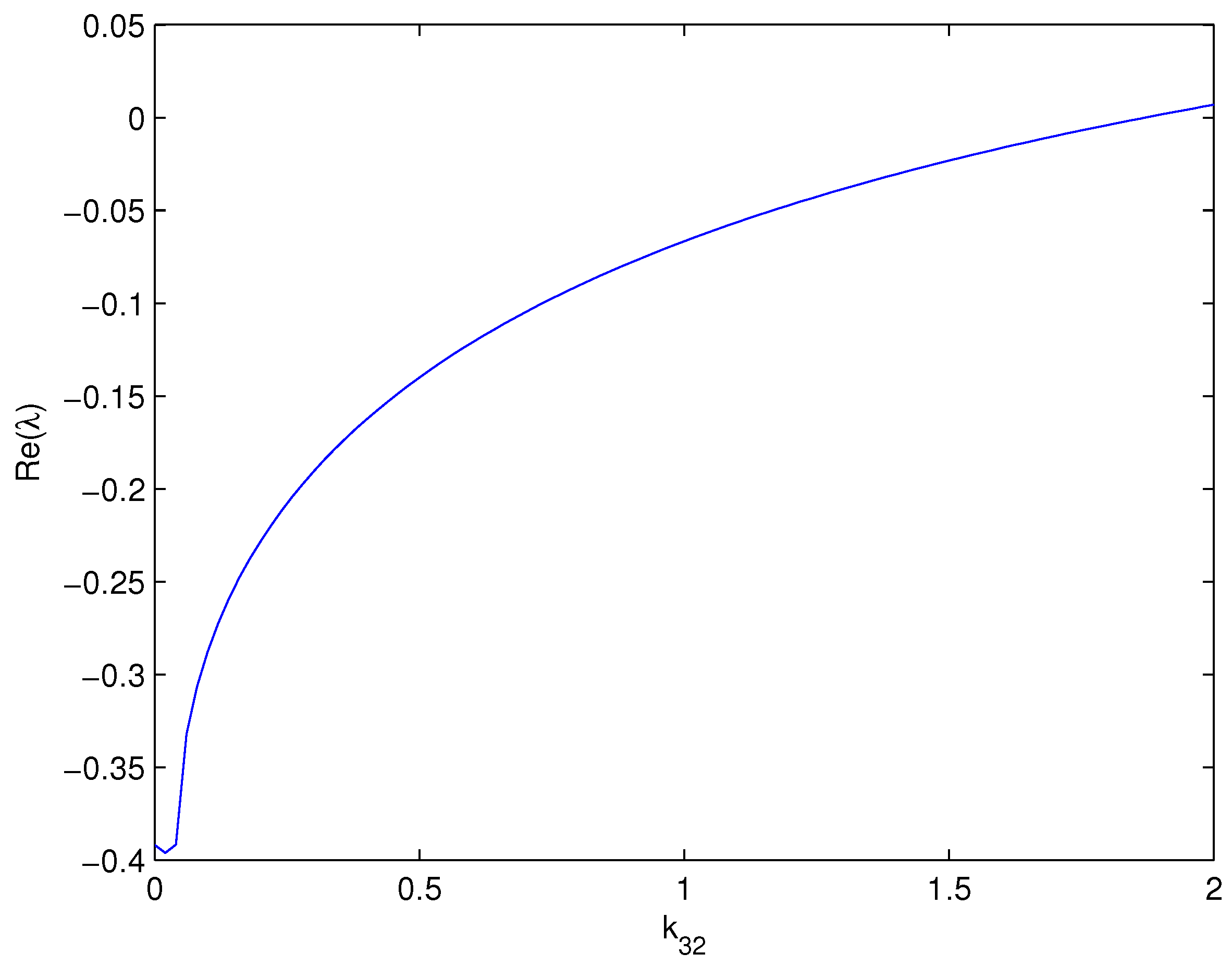
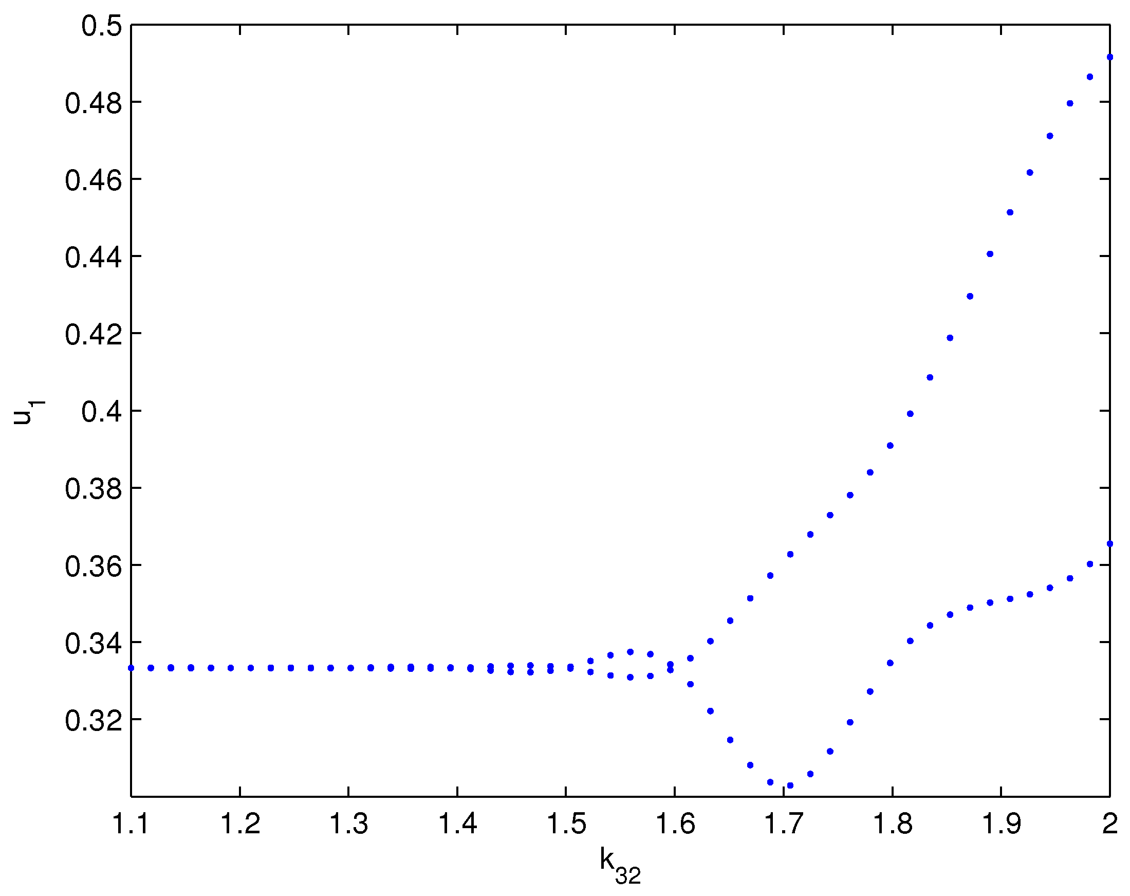
3.2. Effects of Cross-Diffusion on Turing Instability

For simplicity, we denote

$$\mathbf{K}\left(\mathbf{u}\right)=\left(\begin{array}{c}(k_{11}+k_{13}{u}_3)u_1\\ (k_{22}+k_{23}{u}_3)u_2\\ (k_{31}{u}_1+k_{32}{u}_2+k_{33})u_3\end{array}\right),\mathbf{F}\left(\mathbf{u}\right)=\left(\begin{array}{c}a{u}_1(1-u_1)-u_1{u}_3\\ b{u}_2(1-u_2)-u_2{u}_3\\ -c{u}_3^2+(d{u}_1+e{u}_2)u_3\end{array}\right).$$

Then, the reaction–diffusion system (1) can be rewritten in matrix notation as

$$\begin{array}{c}\hfill \left\{\begin{array}{cc}{\displaystyle \frac{\partial \mathbf{u}}{\partial t}-\Delta \mathbf{K}\left(\mathbf{u}\right)=\mathbf{F}\left(\mathbf{u}\right),}\hfill & \mathrm{in}\mathsf{\Omega }\times (0,\infty ),\hfill \\ {\displaystyle \frac{\partial \mathbf{u}}{\partial \eta }=0,}\hfill & \mathrm{on}\mathsf{\Omega }\times (0,\infty ),\hfill \\ \mathbf{u}(x,0)={(u_{10}\left(x\right),u_{20}\left(x\right),u_{30}\left(x\right))}^T,\hfill & \mathrm{in}\mathsf{\Omega }.\hfill \end{array}\right.\end{array}$$

(7)

Linearizing the reaction–diffusion system (7) about the positive equilibrium $\overline{\mathbf{u}}=({\overline{u}}_1,{\overline{u}}_2,{\overline{u}}_3)$, we have

$$\begin{array}{c}\hfill \frac{\partial \mathsf{\Psi }}{\partial t}-{\mathbf{K}}_{\mathbf{u}}\left(\overline{\mathbf{u}}\right)\Delta \mathsf{\Psi }={\mathbf{G}}_{\mathbf{u}}\left(\overline{\mathbf{u}}\right)\mathsf{\Psi },\end{array}$$

(8)

where $\mathsf{\Psi }={({\psi }_1,{\psi }_2,{\psi }_3)}^T$ and

$${\mathbf{K}}_{\mathbf{u}}\left(\mathbf{u}\right)=\left(\begin{array}{ccc}{k}_{11}+k_{13}{\overline{u}}_3& 0& k_{13}{\overline{u}}_1\\ 0& k_{22}+k_{23}{\overline{u}}_3& k_{23}{\overline{u}}_2\\ k_{31}{\overline{u}}_3& k_{32}{\overline{u}}_3& k_{33}+k_{31}{\overline{u}}_1+k_{32}{\overline{u}}_2\end{array}\right),$$

$${\mathbf{G}}_{\mathbf{u}}\left(\mathbf{u}\right)=\left(\begin{array}{ccc}-a{\overline{u}}_1& 0& -{\overline{u}}_1\\ 0& -b{\overline{u}}_2& -{\overline{u}}_2\\ d{\overline{u}}_3& e{\overline{u}}_3& -c{\overline{u}}_3\end{array}\right).$$

Let $0={\mu }_1<{\mu }_2<{\mu }_3<\dots$ be the eigenvalues of the operator $-\Delta$ on $\mathsf{\Omega }$ with the homogeneous Neumann boundary condition, and $E\left({\mu }_i\right)$ be the eigenspace corresponding to ${\mu }_i$ in $C^2\left(\mathsf{\Omega }\right)$. Let $\mathbf{X}=\{\mathbf{u}\in {\left[C^1\left(\overline{\mathsf{\Omega }}\right)\right]}^3|\frac{\partial \mathbf{u}}{\partial \eta }=0\mathrm{on}\partial \mathsf{\Omega }\}$, ${\left\{{\varphi }_{ij}\right\}}_{j=1,2,\dots ,dim E\left({\mu }_i\right)}$ be an orthonormal basis of $E\left({\mu }_i\right)$, and ${\mathbf{X}}_{ij}=\left\{\mathbf{c}{\varphi }_{ij}\right|\mathbf{c}\in {\mathbf{R}}^3\}$. Then,

$$\begin{array}{c}\hfill \mathbf{X}=\underset{i=1}{\overset{\infty }{⨁}}{\mathbf{X}}_i\mathrm{and}{\mathbf{X}}_i=\underset{j=1}{\overset{dim E\left({\mu }_i\right)}{⨁}}{\mathbf{X}}_{ij}.\end{array}$$

For each $i\ge 1$, ${\mathbf{X}}_i$ is invariant under the operator ${\mathbf{K}}_{\mathbf{u}}\left(\overline{\mathbf{u}}\right)\Delta +{\mathbf{G}}_{\mathbf{u}}\left(\overline{\mathbf{u}}\right)$. Then, problem (8) has a non-trivial solution of the form $\mathsf{\Psi }=\mathbf{c}\varphi exp\left(\lambda t\right)$ if and only if $(\lambda ,\mathbf{c})$ is an eigenpair for the matrix $-{\mu }_i{\mathbf{K}}_{\mathbf{u}}\left(\overline{\mathbf{u}}\right)+{\mathbf{G}}_{\mathbf{u}}\left(\overline{\mathbf{u}}\right)$, where $\mathbf{c}$ is a constant vector. Then, the equilibrium $\overline{\mathbf{u}}$ is unstable if at least one eigenvalue $\lambda$ has a positive real part for some ${\mu }_i$.

The characteristic polynomial of $-{\mu }_i{\mathbf{K}}_{\mathbf{u}}\left(\overline{\mathbf{u}}\right)+{\mathbf{G}}_{\mathbf{u}}\left(\overline{\mathbf{u}}\right)$ is given by

$$\begin{array}{c}\hfill {\rho }_i\left(\lambda \right)={\lambda }^3+A_{2i}{\lambda }^2+A_{1i}\lambda +A_{0i},\end{array}$$

(9)

where

$$A_{2i}=(k_{11}+k_{22}+k_{33}+k_{13}{\overline{u}}_3+k_{23}{\overline{u}}_3+k_{31}{\overline{u}}_1+k_{32}{\overline{u}}_2)u_i+a{\overline{u}}_1+b{\overline{u}}_2+c{\overline{u}}_3,$$

(10)

$$\begin{array}{ccc}{A}_{1i}\hfill & =\hfill & [(k_{11}+k_{13}{\overline{u}}_3)(k_{22}+k_{23}{\overline{u}}_3+k_{33}+k_{13}{\overline{u}}_1+k_{32}{\overline{u}}_2)+(k_{22}+k_{23}{\overline{u}}_3)·\hfill \\ \hfill & \hfill & (k_{33}+k_{31}{\overline{u}}_1+k_{32}{\overline{u}}_2)-k_{23}{k}_{32}{\overline{u}}_2{\overline{u}}_3-k_{13}{k}_{31}{\overline{u}}_1{\overline{u}}_3]{\mu }_i^2\hfill \\ \hfill & \hfill & +[(b{\overline{u}}_2+c{\overline{u}}_3)(k_{11}+k_{13}{\overline{u}}_3)+a{\overline{u}}_1(k_{22}+k_{33}+k_{23}{\overline{u}}_3+k_{31}{\overline{u}}_1+k_{32}{\overline{u}}_2)\hfill \\ \hfill & \hfill & +b{\overline{u}}_2(k_{33}+k_{31}{\overline{u}}_1+k_{32}{\overline{u}}_2)+c{\overline{u}}_3(k_{22}+k_{23}{\overline{u}}_3)+{\overline{u}}_2{\overline{u}}_3(k_{23}e-k_{32})\hfill \\ \hfill & \hfill & +{\overline{u}}_1{\overline{u}}_3(k_{13}d-k_{31})]{\mu }_i+a{\overline{u}}_1(b{\overline{u}}_2+c{\overline{u}}_3)+bc{\overline{u}}_2{\overline{u}}_3+e{\overline{u}}_2{\overline{u}}_3+d{\overline{u}}_1{\overline{u}}_3,\hfill \end{array}$$

(11)

$$\begin{array}{ccc}{A}_{0i}\hfill & =\hfill & [(k_{33}{k}_{11}+k_{33}{k}_{13}{\overline{u}}_3+k_{31}{k}_{11}{\overline{u}}_1+k_{31}{\overline{u}}_1{\overline{u}}_3+k_{32}{k}_{11}{\overline{u}}_2+k_{32}{k}_{13}{\overline{u}}_2{\overline{u}}_3)k_{22}\hfill \\ & & +(k_{33}{k}_{11}+k_{33}{k}_{13}{\overline{u}}_3+k_{31}{k}_{11}{\overline{u}}_1)k_{23}]u_i^3+[c{\overline{u}}_3(k_{11}+k_{13}{\overline{u}}_3)(k_{22}+k_{23}{\overline{u}}_3)\hfill \\ & & +(k_{33}+k_{31}+k_{32}{\overline{u}}_2)[a{\overline{u}}_1(k_{22}+k_{23}{\overline{u}}_3)+b{\overline{u}}_2(k_{11}+k_{13}{\overline{u}}_3)]\hfill \\ & & +(k_{11}+k_{13}{\overline{u}}_3)\left(e{k}_{23}{\overline{u}}_2{\overline{u}}_3\right)-a{k}_{23}{k}_{32}{\overline{u}}_1{\overline{u}}_2{\overline{u}}_3+d{k}_{13}{\overline{u}}_1{\overline{u}}_3(k_{22}+k_{23}{\overline{u}}_3)\hfill \\ & & -k_{13}{k}_{31}b{\overline{u}}_1{\overline{u}}_2{\overline{u}}_3-k_{31}{k}_{22}{\overline{u}}_1{\overline{u}}_2-k_{31}{k}_{32}{\overline{u}}_1{\overline{u}}_3^2]{\mu }_i^2+[ac{\overline{u}}_1{\overline{u}}_3(k_{22}+k_{23}{\overline{u}}_3)\hfill \\ & & +bc{\overline{u}}_2{\overline{u}}_3(k_{11}+k_{13}{\overline{u}}_3)+ab{\overline{u}}_1{\overline{u}}_2(k_{33}+k_{31}{\overline{u}}_1+k_{32}{\overline{u}}_2)+e{\overline{u}}_2{\overline{u}}_3(k_{11}\hfill \\ & & +k_{13}{\overline{u}}_3)+a{\overline{u}}_1(e{k}_{23}{\overline{u}}_2{\overline{u}}_3-k_{23}{\overline{u}}_2{\overline{u}}_3)+k_{11}{\overline{u}}_1{\overline{u}}_2{\overline{u}}_{3}bd\hfill \\ & & +d{\overline{u}}_1{\overline{u}}_3(k_{22}+k_{23}{\overline{u}}_3-k_{31}b{\overline{u}}_1{\overline{u}}_2{\overline{u}}_3)]u_i+(abc+ae+bd){\overline{u}}_1{\overline{u}}_2{\overline{u}}_3.\hfill \end{array}$$

(12)

Let ${\lambda }_{1i},{\lambda }_{2i},{\lambda }_{3i}$ be the three roots of (9). In order to obtain the stability of $\overline{\mathbf{u}}$, we need to show that there exists a positive constant $\delta$ such that

$$\begin{array}{c}\hfill Re\left\{{\lambda }_{1i}\right\},Re\left\{{\lambda }_{2i}\right\},Re\left\{{\lambda }_{3i}\right\}<-\delta ,\mathrm{for} \mathrm{all}i\ge 1.\end{array}$$

(13)

The aim of the following theorem is to prove that diffusion alone (without cross-diffusion, i.e., $k_{31}=k_{13}=k_{32}=k_{23}=0$) cannot drive instability for this model.

Theorem 3.

Suppose that (3) holds and $k_{13}=k_{31}=k_{23}=k_{32}=0$. Then, the positive equilibrium $\overline{\mathbf{u}}$ of (7) is linearly stable.

Proof. 

Substituting $k_{13}$ = $k_{31}$ = $k_{23}$ = $k_{32}=0$ into (10)–(12), we have

$$\begin{array}{ccc}\hfill A_{2i}& =& a{\overline{u}}_1+b{\overline{u}}_2+c{\overline{u}}_3+(k_{11}+k_{22}+k_{33}){\mu }_i>0,\hfill \\ \hfill A_{1i}& =& (k_{11}{k}_{22}+k_{11}{k}_{33}+k_{22}{k}_{33}){\mu }_i^2+[a(k_{22}+k_{33}){\overline{u}}_1+b(k_{11}+k_{33}){\overline{u}}_2+c(k_{11}+k_{22}){\overline{u}}_3]{\mu }_i\hfill \\ & & +ab{\overline{u}}_1{\overline{u}}_2+ac{\overline{u}}_1{\overline{u}}_3+d{\overline{u}}_1{\overline{u}}_3+bc{\overline{u}}_2{\overline{u}}_3+e{\overline{u}}_2{\overline{u}}_3>0,\hfill \\ \hfill A_{0i}& =& k_{11}{k}_{22}{k}_{33}{\mu }_i^3+(k_{11}{k}_{22}c{\overline{u}}_3+k_{11}{k}_{33}b{\overline{u}}_2+k_{22}{k}_{33}a{\overline{u}}_1){\mu }_i^2\hfill \\ & & +(ab{k}_{33}{\overline{u}}_1{\overline{u}}_2+d{k}_{22}{\overline{u}}_1{\overline{u}}_2+ac{k}_{22}{\overline{u}}_1{\overline{u}}_3+bc{k}_{11}{\overline{u}}_2{\overline{u}}_3+e{k}_{11}{\overline{u}}_2{\overline{u}}_3+bd{k}_{11}{\overline{u}}_1{\overline{u}}_2{\overline{u}}_3){\mu }_i\hfill \\ & & +(ae+bd+abc){\overline{u}}_1{\overline{u}}_2{\overline{u}}_3>0.\hfill \end{array}$$

A direct calculation shows that $A_{2i}{A}_{1i}-A_{0i}>0$ for all $i\ge 1$. It follows from the Routh–Hurwize criterion that all three roots ${\lambda }_{1i},{\lambda }_{2i},{\lambda }_{3i}$ of ${\rho }_i\left(\lambda \right)=0$ have negative real parts for each $i\ge 1$.

Let $\lambda ={\mu }_i\epsilon$, then

$${\rho }_i\left(\lambda \right)={\mu }_i^3{\xi }^3+A_{2i}{\mu }_i^2{\xi }^2+A_{1i}{\mu }_i\xi +A_{0i}={\tilde{\rho }}_i\left(\xi \right).$$

Since ${\mu }_i\to \infty$, as $i\to \infty$, we have

$$\overline{\rho }\left(\xi \right)=\underset{i\to \infty }{lim}\frac{{\tilde{\rho }}_i\left(\xi \right)}{{\mu }_i^3}={\xi }^3+(k_{11}+k_{22}+k_{33}){\xi }^2+(k_{11}{k}_{22}+k_{22}{k}_{33}+k_{11}{k}_{33})\xi +k_{11}{k}_{22}{k}_{33}.$$

Applying the Routh–Hurwitz criterion, it follows that the three roots ${\xi }_1,{\xi }_2,{\xi }_3$ of $\overline{\rho }\left(\xi \right)=0$ all have negative real parts. Thus, there exists a positive constant $\overline{\delta }$ such that $Re\left\{{\xi }_1\right\},Re\left\{{\xi }_2\right\}$, $Re\left\{{\xi }_3\right\}\le -2\overline{\delta }$. By continuity, we see that there exists $i_0\ge 1$, such that ${\mu }_{i0}>1$ and the three roots ${\xi }_{i1},{\xi }_{i2},{\xi }_{i3}$ of ${\tilde{\rho }}_i\left(\xi \right)=0$ satisfy $Re\left\{{\xi }_{i1}\right\},Re\left\{{\xi }_{i2}\right\}$, $Re\left\{{\xi }_{i3}\right\}\le -{\mu }_i\overline{\delta }\le -{\mu }_{i0}\overline{\delta }\le -\overline{\delta }$ for any $i\ge i_0$. Let $-\tilde{\delta }={max}_{1\le i\le i_0}\{Re\left\{{\lambda }_{i1}\right\},Re\left\{{\lambda }_{i2}\right\},Re\left\{{\lambda }_{i3}\right\}\}$ and $\delta =min\{\tilde{\delta },\overline{\delta }\}$, then (13) holds. Consequently, the equilibrium $\overline{\mathbf{u}}$ is linearly stable. □

Note that $A_{2i}>0,A_{1i}>0,A_{0i}>0$ and $A_{2i}{A}_{1i}-A_{0i}>0$ if $k_{31}=k_{32}=0$ since the possible negative terms all involve either $k_{31}$ or $k_{32}$. By the same arguments as in Theorem 3, we have

Theorem 4.

Suppose that (3) holds and $k_{31}=k_{32}=0$, Then, the positive equilibrium $\overline{\mathbf{u}}$ of (1) is linearly stable.

Next, we consider the Turing instability, i.e., the stability of the positive equilibrium $\overline{u}=({\overline{u}}_1,{\overline{u}}_2,{\overline{u}}_3)$ changing from stable for the ODE dynamics (2), to unstable for the PDE dynamics (1). Here, we give sufficient conditions for cross-diffusion, which drives the instability, and $k_{31}$ and $k_{32}$ are chosen as variation parameters.

Theorem 5.

$\left(1\right)$ Suppose that $a{\overline{u}}_1-{\overline{u}}_3<0$. Consider $k_{31}$ as the variation parameter; then, there exists a positive constant ${\delta }_{31}$ such that when $k_{31}>{\delta }_{31}$, the equilibrium $\overline{\mathbf{u}}$ is linearly unstable for some domain Ω.

• $\left(2\right)$ Suppose that $b{\overline{u}}_2-{\overline{u}}_3<0$. Consider $k_{32}$ as the variation parameter; then, there exists a positive constant ${\delta }_{32}$ such that when $k_{32}>{\delta }_{32}$, the equilibrium $\overline{\mathbf{u}}$ is linearly unstable for some domain Ω.

Proof. 

Denote

$$\begin{array}{c}\hfill A\left(\mu \right)=-(C_3{\mu }^3+C_2{\mu }^2+C_1\mu +C_0),\end{array}$$

(14)

where

$$\begin{array}{ccc}\hfill C_3& =& [(k_{33}{k}_{11}+k_{33}{k}_{13}{\overline{u}}_3+k_{31}{k}_{11}{\overline{u}}_1+k_{31}{\overline{u}}_1{\overline{u}}_3+k_{32}{k}_{11}{\overline{u}}_2+k_{32}{k}_{13}{\overline{u}}_2{\overline{u}}_3)k_{22}\hfill \\ & & +(k_{33}{k}_{11}+k_{33}{k}_{13}{\overline{u}}_3+k_{31}{k}_{11}{\overline{u}}_1)k_{23}],\hfill \\ \hfill C_2& =& [c{\overline{u}}_3(k_{11}+k_{13}{\overline{u}}_3)(k_{22}+k_{23}{\overline{u}}_3)+(k_{33}+k_{31}+k_{32}{\overline{u}}_2)[a{\overline{u}}_1(k_{22}+k_{23}{\overline{u}}_3)\hfill \\ & & +b{\overline{u}}_2(k_{11}+k_{13}{\overline{u}}_3)]+(k_{11}+k_{13}{\overline{u}}_3)\left(e{k}_{23}{\overline{u}}_2{\overline{u}}_3\right)-a{k}_{23}{k}_{32}{\overline{u}}_1{\overline{u}}_2{\overline{u}}_3\hfill \\ & & +d{k}_{13}{\overline{u}}_1{\overline{u}}_3(k_{22}+k_{23}{\overline{u}}_3)-k_{13}{k}_{31}b{\overline{u}}_1{\overline{u}}_2{\overline{u}}_3-k_{31}{k}_{22}{\overline{u}}_1{\overline{u}}_2-k_{31}{k}_{32}{\overline{u}}_1{\overline{u}}_3^2],\hfill \\ \hfill C_1& =& [ab{\overline{u}}_1{\overline{u}}_2{k}_{31}(a{\overline{u}}_1-{\overline{u}}_3)+a{\overline{u}}_1{\overline{u}}_2{k}_{32}(b{\overline{u}}_2-{\overline{u}}_3)+ac{\overline{u}}_1{\overline{u}}_3(k_{22}+k_{23}{\overline{u}}_3)+\hfill \\ & & bc{\overline{u}}_2{\overline{u}}_3(k_{11}+k_{13}{\overline{u}}_3)+ab{\overline{u}}_1{\overline{u}}_2{k}_{33}+e{\overline{u}}_2{\overline{u}}_3(k_{11}+k_{13}{\overline{u}}_3)+ae{k}_{23}{\overline{u}}_1{\overline{u}}_2{\overline{u}}_3\hfill \\ & & +k_{11}bd{\overline{u}}_1{\overline{u}}_2{\overline{u}}_3+d{\overline{u}}_1{\overline{u}}_3(k_{22}+k_{23}{\overline{u}}_3),\hfill \\ \hfill C_0& =& (abc+ae+bd){\overline{u}}_1{\overline{u}}_2{\overline{u}}_3.\hfill \end{array}$$

Case 1: $k_{31}$ is the variation parameter.

We assume that $a{\overline{u}}_1-{\overline{u}}_3<0$. The following arguments by continuation are based on the fact that each root of the algebraic Equation (14) is a continuous function of the variation parameter $k_{31}$. It is easy to prove that Equation (14) has three real roots ${\mu }_1^{\left(i\right)}={\mu }_1^{\left(i\right)}\left(k_{31}\right)$, $i=1,2,3$ when $k_{31}$ goes to infinity and they satisfy ${lim}_{k_{31}\to \infty }{\mu }_1^{\left(1\right)}\left(k_{31}\right)<0$, ${lim}_{k_{31}\to \infty }{\mu }_1^{\left(2\right)}\left(k_{31}\right)=0$ and ${lim}_{k_{31}\to \infty }{\mu }_1^{\left(3\right)}\left(k_{31}\right)>0$. By continuation, there exists a positive constant ${\delta }_{31}$ such that when $k_{31}>{\delta }_{31}$, $C_1>0$, and $det\left(A\right(\mu \left)\right)$ has three real roots. Because $C_3>0$ and $C_0>0$, the number of sign changes in (14) is exactly two. Therefore, by Descartes’ rule, the three real roots have the following properties:

(1)

$-\infty <{\mu }_1^{\left(1\right)}<0<{\mu }_1^{\left(2\right)}<{\mu }_1^{\left(3\right)}<\infty ,$

(2)

$\det \left(A\right(\mu \left)\right)>0$ if $\mu \in (-\infty ,{\mu }_1^{\left(1\right)})\cup ({\mu }_1^{\left(2\right)},{\mu }_1^{\left(3\right)}),$

(3)

$\det \left(A\right(\mu \left)\right)<0$ if $\mu \in ({\mu }_1^{\left(1\right)},{\mu }_1^{\left(2\right)})\cup ({\mu }_1^{\left(3\right)},\infty ).$

If ${\mu }_i\in ({\mu }_1^{\left(2\right)},{\mu }_1^{\left(3\right)})$ for some i, then $det\left(A\left({\mu }_i\right)\right)>0$ by (2), and, consequently, $A_{0i}=-det\left(A_{\left(i\right)}\right)<0$. The number of sign of changes in the characteristic polynomial (9) ${\rho }_i\left(\lambda \right)={\lambda }^3+A_{2i}{\lambda }^2+A_{1i}\lambda +A_{0i}$ is either one or three. By Descartes’ rule, the characteristic polynomial (9) has at least one positive eigenvalue. Hence, the equilibrium $\overline{\mathbf{u}}$ of (1) is linearly unstable for any domain $\mathsf{\Omega }$ on which at least one eigenvalue ${\mu }_i$ of $-\Delta$ is in the interval $({\mu }_1^{\left(2\right)},{\mu }_1^{\left(3\right)})$.

Case 2: $k_{32}$ is the variation parameter.

We assume that $b{\overline{u}}_2-{\overline{u}}_3<0$. The following arguments by continuation are based on the fact that each root of Equation (14) is a continuous function of the variation $k_{32}$. It is easy to prove that Equation (14) has three real roots ${\mu }_2^{\left(i\right)}={\mu }_2^{\left(i\right)}\left(k_{32}\right)$, $i=1,2,3$ when $k_{32}$ goes to infinity and they are ${lim}_{k_{32}\to \infty }{\mu }_2^{\left(1\right)}\left(k_{32}\right)<0$, ${lim}_{k_{32}\to \infty }{\mu }_2^{\left(2\right)}\left(k_{32}\right)=0$ and ${lim}_{k_{32}\to \infty }{\mu }_2^{\left(3\right)}\left(k_{32}\right)>0$. By continuation, there exists a positive constant ${\delta }_{32}$ such that when $k_{32}>{\delta }_{32}$, $C_1>0$, and $det\left(A\right(\mu \left)\right)$ has three real roots. Because $C_3>0$ and $C_0>0$, the number of sign changes in (14) is exactly two. Therefore, by Descartes’ rule, the three real roots have the following properties:

(1)

$-\infty <{\mu }_2^{\left(1\right)}<0<{\mu }_2^{\left(2\right)}<{\mu }_2^{\left(3\right)}<\infty$,

(2)

$det\left(A\left(\mu \right)\right)>0if\mu \in (-\infty ,{\mu }_2^{\left(2\right)})\bigcup ({\mu }_2^{\left(2\right)},{\mu }_2^{\left(3\right)})$,

(3)

$det\left(A\left(\mu \right)\right)<0if\mu \in ({\mu }_2^{\left(1\right)},{\mu }_2^{\left(2\right)})\bigcup ({\mu }_2^{\left(3\right)},\infty )$.

If ${\mu }_i\in ({\mu }_2^{\left(2\right)},{\mu }_2^{\left(3\right)})$ for some i, then $det\left(A\left({\mu }_i\right)\right)>0$, and, consequently, $A_{0i}=-det\left(A_{\left(i\right)}\right)$$<0$. By similar argument as in case 1, the number of sign changes in the characteristic polynomial (9) ${\rho }_i\left(\lambda \right)={\lambda }^3+A_{2i}{\lambda }^2+A_{1i}\lambda +A_{0i}$ is either one or three. By Descartes’ rule, the characteristic polynomial (9) has at least one positive eigenvalue. Hence, the equilibrium $\overline{u}$ of (1) is linearly unstable for any domain $\mathsf{\Omega }$ on which at least one eigenvalue ${\mu }_i$ of $-\Delta$ is in the interval $({\mu }_2^{\left(2\right)},{\mu }_2^{\left(3\right)})$. □

Remark 1.

$\left(i\right)$ In Theorem 5, the conditions $a{\overline{u}}_1-{\overline{u}}_3<0$ and $b{\overline{u}}_2-{\overline{u}}_3<0$ are compatible with the condition (3), respectively.

• $\left(ii\right)$ $k_{31}$ and $k_{32}$ can be chosen as variation parameters because the number of sign changes for the polynomial (14) could be bigger than one for large values of $k_{31}$ or $k_{32}$. By Descartes’ rule, the polynomial (14) could have positive roots which lead to linear instability.
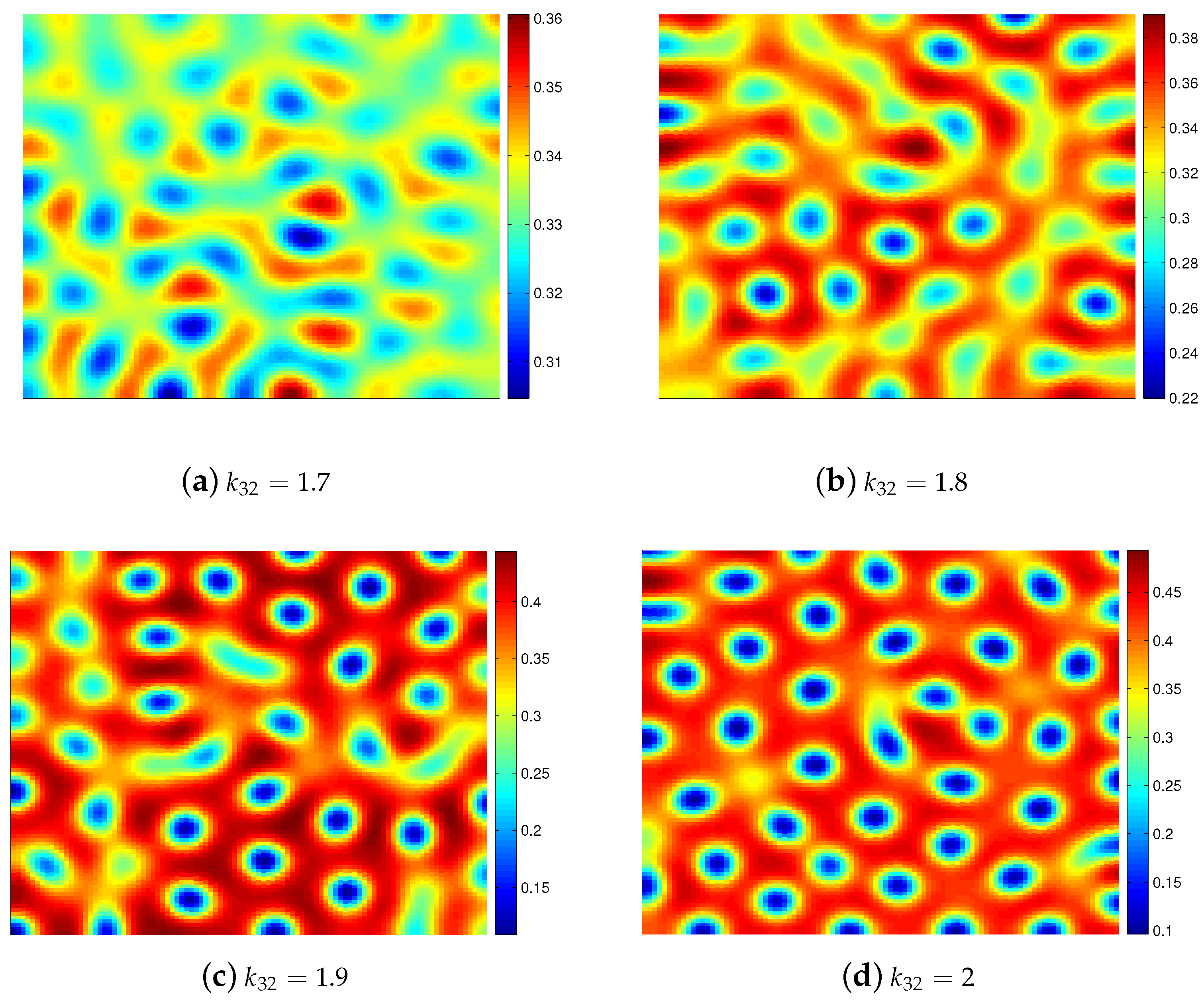
• $\left(iii\right)$ Biological interpretation: In our model, the third species preys on the first and second. The positive steady state of the model can be broken by the reaction–diffusion among two species in the model.

Case one: In this case, the first species is assumed to reproduce exponentially unless subject to intraspecies competition and predation. This exponential growth is represented in the equation by the term $a{u}_1$. The level of intraspecies competition among the first species is assumed to be proportional to the population density of the first species by the term $a{u}_1$. The rate of predation upon the prey is assumed to be proportional to the rate at which the predators and the prey meet by the term $u_1{u}_3$, when the effects on the first species due to the fact that the third species preys on the first one ${\overline{u}}_3$ are larger than the effects on the first species due to intraspecies competition $a{\overline{u}}_1$. The large cross-diffusion of the third species due to the first species $k_{31}$ can break the stability of the positive steady state. In other words, if the predator has a dominant effect on the decrease in prey numbers, such as the predation rate being higher than the rate of intraspecies competition, then the predator with large cross-diffusion can destabilize the constant steady state.

Case two: In this case, the third species has a dominant effect on the decrease in the second species. Because $b{\overline{u}}_2-{\overline{u}}_3<0$ implies $b{\overline{u}}_2<{\overline{u}}_3$, the predation rate of the third species on the second species is higher than the rate of intraspecies competition in second species. A similar situation to that in case one happens in case two: the predator with large cross-diffusion can destabilize the constant steady state.

4. Numerical Simulations

In this section, using the standard finite difference method and perturbation method based on the software MATLAB, we illustrate that cross-diffusion induces spatial patterns. The initial data are taken as a uniformly distributed random perturbation around the equilibrium state $({\overline{u}}_1,{\overline{u}}_2,{\overline{u}}_3)$ in $\mathsf{\Omega }$, with a variance lower than the amplitude of the final pattern. More precisely,

$$\begin{array}{c}\hfill u_{10}\left(x\right)={\overline{u}}_1+{\eta }_1\left(x\right),u_{20}\left(x\right)={\overline{u}}_2+{\eta }_2\left(x\right),u_{30}\left(x\right)={\overline{u}}_3+{\eta }_3\left(x\right),\end{array}$$

where ${\eta }_i\in [-1.5,1.5]$ for $i=1,2,3$. In view of Theorems 3 and 5, the Turing parameter space is (3), under which spatial patterns can occur. Thus, in system (1), we fix $a=1$, $b=1$, $c=0.1$, $d=0.1$, $e=0.1$, $k_{11}=0.1$, $k_{13}=0.1$, $k_{22}=0.1$, $k_{23}=0.1$, $k_{31}=0.1$ and $k_{33}=0.1$.

In Figure 1, we show the real part of the eigenvalue $\lambda$ as a function of the cross-diffusion coefficient $d_{32}$. From the characteristic polynomial of (9), we can determine the value of $d_{32}$ such that $Re\left(\lambda \right)>0$. Now, we will implement some numerical simulations for the system (1). The domain is confined to a square domain $\mathsf{\Omega }=[0,L_x]\times [0,L_y]\subset {\mathbf{R}}^2$. The wave number for this two-dimensional domain is thereby

$$\mathbf{k}=\pi (m/L_x,n/L_y),\mathrm{and}\left|\mathbf{k}\right|=\pi \sqrt{{(m/L_x)}^2+{(n/L_y)}^2},m,n=0,1,\dots .$$

We consider system (1) in a fixed domain, $L_x=40$ and $L_y=40$, and resolve it on a grid with $100\times 100$ sites with the space step of $▵x=▵y=1$. For the evolution over time, we apply a first-order backward Euler time-advancing scheme with a time step $▵t=0.005$. By discretizing the Laplacian in the grid with lattice sites denoted by $(i,j)$, the nine-point formula is

$$\begin{array}{cc}\hfill {▵u|}_{(i,j)}& =\frac{1}{6▵x^2}[4a_l(i,j)u(i-1,j)+4a_r(i,j)u(i+1,j)+4a_d(i,j)u(i,j-1)\hfill \\ & +4a_u(i,j)u(i,j+1)+a_l(i,j)u(i-1,j+1)+a_u(i,j)u(i+1,j+1)\hfill \\ & \hspace{1em} +a_d(i,j)u(i-1,j-1)+a_r(i,j)u(i+1,j-1)-20u(i,j)],\hfill \end{array}$$

where the matrix elements of $a_l,a_r,a_d,a_u$ are united, except at the boundary. When $(i,j)$ is at the left boundary, that is, $i=0$, we define $a_l(i,j)u(i-1,j)\equiv u(i+1,j)$, which guarantees the zero-flux of reactants in the left boundary. Similarly we define $a_r(i,j)$, $a_d(i,j)$, and $a_u(i,j)$ such that the boundary is no-flux. The nine-point formula for the Laplacian can have a one-step error of $O(▵x^4)$.

In Figure 2, we compare the density of $u_1$ before and after the onset of Turing patterns. The results are qualitatively similar for $u_2$ and $u_3$, and hence are omitted. In the case of $k_{32}$ less than 1.6, i.e., the Turing instability does not occur, we see that the density of $u_1$ is homogeneous. In the case of $k_{32}$ larger than 1.6, i.e., the Turing instability occurs, we see that the density of $u_1$ is spatially inhomogeneous.

Now, we study the change in the spatial patterns qualitatively and quantitatively with different $k_{32}$. In general, the selection of a stripe pattern or spot pattern depends upon the non-linearities of the reaction kinetics. Specifically, it has been shown that the presence of quadratic non-linearities in the reaction kinetics leads to the spot pattern, but the absence of quadratic terms leads to the stripe pattern [30]. Noticing that the reaction kinetics of (1) only contain quadratic non-linearities, in view of the theory of pattern selection [30], all of the spatial patterns are spot patterns. In Figure 3, we also illustrate the quantitative change in the spatial patterns with different values of $k_{32}$. From these simulations, we can conclude that with the increase in $k_{32}$, the spatial patterns of $u_1$ converge to regular spotted patterns. The striped patterns cannot occur in our model.

5. Conclusions

In this paper, we develop a theoretical framework for studying the phenomenon of pattern formation in a two-prey one-predator system. Applying stability analysis and suitable numerical simulations, we investigate the Turing parameter space, the associated pattern type and the Turing bifurcation diagram.

Our results indicate that the unique positive equilibrium solution is globally asymptotically stable for the corresponding kinetic system (the system without diffusion) and remains locally linearly stable for the reaction–diffusion system without cross-diffusion; hence, it does not belong to the classical Turing instability scheme. Moreover, we prove that the positive equilibrium solution is globally asymptotically stable for the reaction–diffusion system without cross-diffusion. However, it becomes linearly unstable only when non-linear cross-diffusion also plays a role in the reaction–diffusion system; thus, it is cross-diffusion-induced instability, which is demonstrated by the corresponding numerical simulations.

6. Discussion

It is worth mentioning that the authors have also investigated the role of cross-diffusion in pattern formation for Lotka–Volterra-type models in [31,32]. In [32], by considering a Holling–Tanner predator–prey model, the authors investigated the Turing bifurcation and obtained the pattern selection mechanism. In [31], by studying the Hopf bifurcation, the authors attained the spiral patterns. Apart from these works [31,32], what our model considers is a three-species model. The difficulty is that the characteristic equation of our model is a cubic equation. We use the continuity of the cubic functions to overcome it. The novelty of this work is that we obtain the bifurcation diagram for the Turing onset by numerical simulations, which shows the transition from the homogeneous steady state to the Turing patterns.

The proposed approach has applicability to other reaction–diffusion systems, including cross-diffusion, such as chemotaxis and cell motility models. In this context, it is of great interest to study the development of a general mathematical and numerical framework that allows for the treatment of certain degenerate quasilinear parabolic systems modeling bacterial growth, which are known to involve several important phenomena such as fractal morphogenesis and branching patterns. In conclusion, we propose that the emergence of complex spatio-temporal dynamics in predator–prey models may be attributed to cross-diffusion. Furthermore, the approach proposed in continuous spaces can also be extended to finite weighted networks and a corresponding theory of pattern formation can also be established.

References

1. Turing, A.M. The chemical basis of morphogenesis. Philos. Trans. R. Soc. Lond. Ser. B 1952, 237, 37–72. [Google Scholar]
2. Cintra, W.; dos Santos, C.A.; Zhou, J.Z. Coexistence states of a Holling type II predator-prey system with self and cross-diffusion terms. Discret. Contin. Dyn. Syst. Ser. B 2022, 27, 3913–3931. [Google Scholar] [CrossRef]
3. Farshid, M.; Jalilian, Y. Steady state bifurcation in a cross diffusion prey-predator model. Comput. Methods Differ. Equ. 2023, 11, 254–262. [Google Scholar] [CrossRef]
4. Kuto, K. Stability of steady-state solutions to a prey-predator system with cross-diffusion. J. Differ. Equ. 2004, 197, 293–314. [Google Scholar] [CrossRef]
5. Kuto, K.; Yamada, Y. Multiple coexistence states for a prey-predator system with cross-diffusion. J. Differ. Equ. 2004, 197, 315–348. [Google Scholar] [CrossRef]
6. Li, Q.; He, J.F. Pattern formation in a ratio-dependent predator-prey model with cross diffusion. Electron. Res. Arch. 2023, 31, 1106–1118. [Google Scholar] [CrossRef]
7. Ling, Z.; Zhang, L.; Lin, Z.G. Turing pattern formation in a predator-prey system with cross diffusion. Appl. Math. Model. 2014, 38, 5022–5032. [Google Scholar] [CrossRef]
8. Ma, L.; Wang, H.T.; Gao, J.P. Dynamics of two-species Holling type-II predator-prey system with cross-diffusion. J. Differ. Equ. 2023, 365, 591–635. [Google Scholar] [CrossRef]
9. Peng, R.; Wang, M.X.; Yang, G.Y. Stationary patterns of the Holling-Tanner prey-predator model with diffusion and cross-diffusion. Appl. Math. Comput. 2008, 196, 570–577. [Google Scholar] [CrossRef]
10. Tao, Y.S.; Winkler, M. Existence theory and qualitative analysis for a fully cross-diffusive predator-prey system. SIAM J. Math. Anal. 2022, 54, 4806–4864. [Google Scholar] [CrossRef]
11. Wang, M.X. Stationary patterns caused by cross-diffusion for a three-species prey-predator model. Comput. Math. Appl. 2006, 52, 707–720. [Google Scholar] [CrossRef]
12. Xie, Z.F. Cross-diffusion induced Turing instability for a three species food chain model. J. Math. Anal. Appl. 2012, 388, 539–547. [Google Scholar] [CrossRef]
13. Zhu, M.; Li, J.; Lian, X. Pattern Dynamics of Cross Diffusion Predator–Prey System with Strong Allee Effect and Hunting Cooperation. Mathematics 2022, 10, 3171. [Google Scholar] [CrossRef]
14. Kerner, E.H. Further considerations on the statistical mechanics of biological associations. Bull. Math. Biophys. 1959, 21, 217–255. [Google Scholar] [CrossRef]
15. Shigesada, N.; Kawasaki, K.; Teramoto, E. Spatial segregation of interacting species. J. Theoret. Biol. 1979, 79, 83–99. [Google Scholar] [CrossRef]
16. Prokopev, S.; Lyubimova, T.; Mialdun, A.; Shevtsova, V. A ternary mixture at the border of Soret separation stability. Phys. Chem. Chem. Phys. 2021, 23, 8466–8477. [Google Scholar] [CrossRef] [PubMed]
17. Šeta, B.; Errarte, A.; Ryzhkov, I.I.; Bou-Ali, M.M.; Shevtsova, V. Oscillatory instability caused by the interplay of Soret effect and cross-diffusion. Phys. Fluids 2023, 35, 021702. [Google Scholar] [CrossRef]
18. Vanag, V.K.; Epstein, I.R. Cross-diffusion and pattern formation in reaction–diffusion systems. Phys. Chem. Chem. Phys. 2009, 11, 897–912. [Google Scholar] [CrossRef]
19. Jorné, J. The diffusive Lotka-Volterra oscillating system. J. Theor. Biol. 1977, 65, 133–139. [Google Scholar] [CrossRef]
20. Kersner, R.; Klincsik, M.; Zhanuzakova, D. A competition system with nonlinear cross-diffusion: Exact periodic patterns. Rev. R. Acad. Cienc. Exactas Fís. Nat. Ser. A Mat. 2022, 116, 187. [Google Scholar] [CrossRef]
21. Matano, H.; Mimura, M. Pattern formation in competion-diffusion systems in nonconvex domains. Publ. Res. Inst. Math. Sci. 1983, 19, 1049–1079. [Google Scholar] [CrossRef]
22. Gurtin, M.E. Some mathematical models for population dynamics that lead to segregation. Quart. Appl. Math. 1974, 32, 1–9. [Google Scholar] [CrossRef]
23. Dhariwal, G.; Jüngel, A.; Zamponi, N. Global martingale solutions for a stochastic population cross-diffusion system. Stoch. Process Their Appl. 2019, 129, 3792–3820. [Google Scholar] [CrossRef]
24. Yamada, Y. Global solutions for quasilinear parabolic systems with cross-diffusion effects. Nonlinear Anal. 1995, 24, 1395–1412. [Google Scholar] [CrossRef]
25. Elettreby, M.F. Two-prey one-predator model. Chaos Solitons Fractals 2009, 39, 2018–2027. [Google Scholar] [CrossRef]
26. Cantrell, R.S.; Cosner, C. Spatial Ecology via Reaction-Diffusion Equations; John Wiley & Sons, Ltd.: Chichester, UK, 2003. [Google Scholar]
27. Lou, Y.; Ni, W.M. Diffusion, self-diffusion and cross-diffusion. J. Differ. Equ. 1996, 131, 79–131. [Google Scholar] [CrossRef]
28. Okubo, A. Diffusion and Ecological Problems: Mathematical Models; Springer: Berlin/Heidelberg, Germany; New York, NY, USA, 1980. [Google Scholar]
29. Hale, J.K. Ordinary Differential Equations; Krieger: Malabar, FL, USA, 1980. [Google Scholar]
30. Ermentrout, B. Stripes or spots? Non-linear effects in bifurcation of reaction-diffusion equations on the square. Proc. R. Soc. Lond. A 1991, 434, 413–417. [Google Scholar] [CrossRef]
31. Guin, L.N.; Haque, M.; Mandal, P.K. The spatial patterns through diffusion-driven instability in a predator-prey model. Appl. Math. Model. 2012, 36, 1825–1841. [Google Scholar] [CrossRef]
32. Sun, G.Q.; Jin, Z.; Li, L.; Haque, M.; Li, B.-L. Spatial patterns of a predator-prey model with cross diffusion. Nonlinear Dynam. 2012, 69, 1631–1638. [Google Scholar] [CrossRef]
Figure 1. Dispersion relationship for the real part of the eigenvalues, Re ( λ ) , versus the cross-diffusion coefficient, k 32 .
Mathematics 11 02411 g001
Figure 2. Bifurcation diagram for Turing onset. Maximum and minimum of u 1 for different levels of cross-diffusion in the transition from the homogeneous state to the Turing pattern.
Mathematics 11 02411 g002
Figure 3. Spatial patterns of u 1 change quantitatively with different k 32 values of 1.7, 1.8, 1.9, and 2. The other parameters are stated in the text. The number of iteration steps for time is 40,000.
Mathematics 11 02411 g003
Disclaimer/Publisher’s Note: The statements, opinions and data contained in all publications are solely those of the individual author(s) and contributor(s) and not of MDPI and/or the editor(s). MDPI and/or the editor(s) disclaim responsibility for any injury to people or property resulting from any ideas, methods, instructions or products referred to in the content.