1. Introduction
With the impact of the recent coronavirus disease 2019 (COVID-19) pandemic, there is an urgent need for rapid testing and screening to confirm whether individuals are infected. However, the large number of screening samples has overwhelmed the manpower of medical institutions. To speed up disease detection, alternative methods such as quick screening reagents are being adopted. The high number of COVID-19 patients worldwide is causing a considerable burden on the global healthcare system. Consequently, many studies have been conducted on medical and healthcare applications using deep learning (DL) for coronavirus detection. For instance, COVID-Net [
1] developed a new Deep Neural Network (DNN) model to detect coronavirus from lung X-ray images. In another study [
2], ImageNet [
3] was used as a pre-trained model for transfer learning. The model was further combined with COVID-Net to train chest computed tomography (CT) images and investigate the performance effect of initial model parameters. However, resource-deficient institutions may face inefficiencies due to an insufficient quantity of data.
To train the model effectively, medical data are usually uploaded to a server. Traditional DL approaches rely on centralized learning (CL), where all data are collected on a server for storage and training. However, in practical scenarios, medical institutions face privacy issues when using CL technologies. The collected datasets may contain sensitive data, such as X-rays, facial data, or disease history. During the training process, data may be accidentally leaked, and sensitive information may indirectly identify user characteristics. Therefore, privacy concerns regarding patient data are rising among medical institutions.
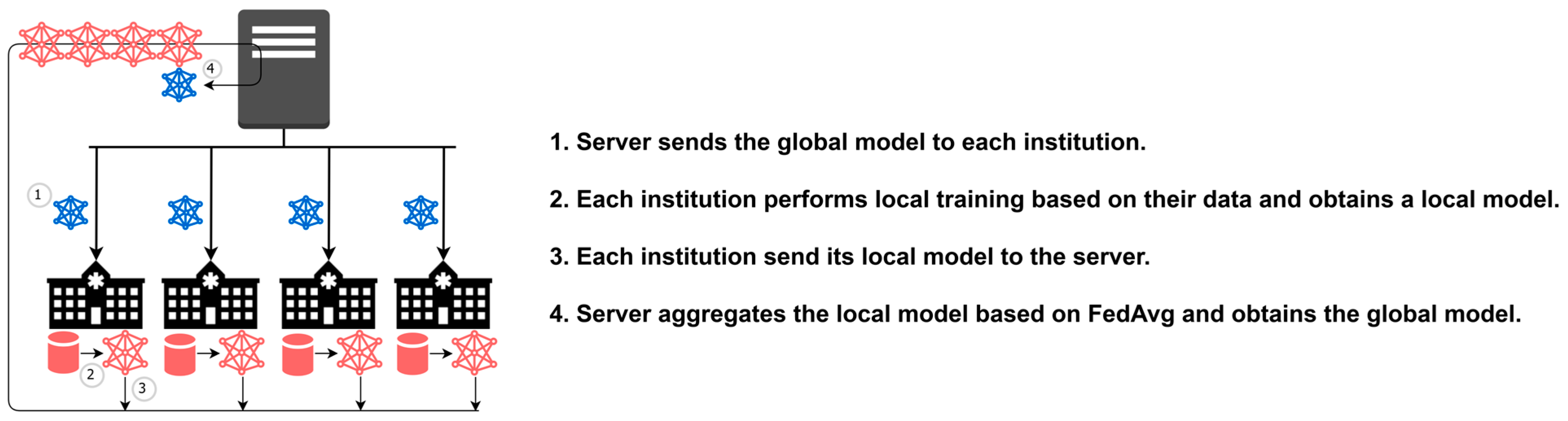
To address privacy concerns in CL, the federated learning (FL) approach has been proposed in recent years. FL is an emerging collaborative framework for distributed machine learning, as shown in
Figure 1. The FedAvg [
4] algorithm, represented in Equation (1), obtains the global model
wt by averaging the local model
wit of each institution
i. The standard optimization formulation in FL is shown in Equation (2), where F() is the loss function and
wit represents the model of each institution
i. The ultimate objective is to aggregate a model that can fit the data of each institution and minimize the sum of the obtained loss values.
Unlike CL, the FL training process does not require pooling raw data to a centralized server or exchanging raw data between clients. In other words, medical institutions do not have to send out their patient data, which alleviates privacy issues. Instead, clients exchange only model parameters and metadata during the training process. Resource-deficient institutions can also benefit from FL aggregation by exchanging learning features with other institutions. Each institution may learn different features from different datasets in other institutions, resulting in improved overall performance. Finally, medical personnel from each institution can assess the results through the model inference.
Sharing data between medical institutions is a sensitive matter, especially when the data contain private patient information. During the transmission process, the data may be vulnerable to network attacks or leaks [
5]. Therefore, regulations such as General Data Protection Regulation (GDPR) [
6] have been enacted to protect the personal data of European citizens. Collecting user data in a proper and lawful manner is essential to obtain user consent.
Without sending data to the server, the performance of FL highly depends on the completeness of data in each institution. Due to data privacy, the server cannot access the raw data of the institution, which brings many challenges in FL [
4], such as Non-Independent Identically Distribution (Non-IID), imbalanced dataset distribution, massively distributed participants, and limited communication rounds. Among these challenges, data imbalance is the key factor affecting the performance of the training model. Some approaches have also been proposed to improve the FedAvg approach in classical FL. FedProx [
7] adapted an optimizer to make the model gradient updates smaller. FedNova [
8] referred to the training step and the quantity of data needed to improve the aggregator. Federated Stochastic Gradient Descent COVID-19 Detection (FedSGDCOVID) [
9] combined FedAvg with the Differential Privacy Stochastic Gradient Descent (DP-SGD) [
10] algorithm to improve the FL security by adding randomized Gaussian noise to the local gradient during the aggregation step. DataSilos [
11] integrated the above approaches to conduct the experiment based on the same benchmark. However, none of the state-of-the-art approaches have particularly outstanding performance in the Non-IID environment. Another experiment [
12] conducted on five advanced algorithms also concluded that Non-IID has a significant impact on FL.
On the other hand, data imbalance problems often occur in healthcare scenarios. Various frameworks for distributed DL were proposed in previous works, such as Institutional Incremental Learning (IIL) and Cyclic Institutional Incremental Learning (CIIL) [
13,
14]. Experiments were conducted on these frameworks to explore the catastrophic forgetting problem [
15] in FL. In other medical applications, FL aids in learning feature extraction for depression [
16]. The authors proposed a face detection and speech emotional classifier using a Convolutional Neural Network (CNN) combined with a Support Vector Machine (SVM). FL calculates a patient sentiment factor based on the label probability to provide advice for professionals to make a complete assessment. In contrast, the authors [
17] adopted an FL framework to build a breast density classification model using mammography data. The model inference for breast density is an important factor that directly affects the diagnosis. However, their work lacked data heterogeneity and may be inefficient in the Non-IID environment.
The shared data approach [
18] can effectively alleviate data imbalance by allowing the server to collect shared data from institutions for data expansion during training. However, in medical scenarios, exchanging raw data is discouraged due to privacy concerns. Therefore, this paper proposes a novel shared model approach for FL called FedISM, which enhances data imbalance without requiring the exchange of shared data. FedISM not only alleviates the problem of data imbalance distribution without exchanging shared data, but it also improves test accuracy with a shared model. Additionally, FL lacks an appropriate factor to assess the completeness of a dataset. It is imperative to delve into the realm of mathematics to determine which factors are appropriate for evaluating datasets in FL. However, some evaluation factors, such as computational power, have been studied in FedCS [
19]. The main goal of FedCS is to explore ways of completing training within a specified time frame in a heterogeneous computing environment. Participants with large datasets may give up due to the long computation time. Therefore, the field of federated learning currently lacks a solution to efficiently evaluate datasets among participants. Accordingly, a Candidate Selection Mechanism (CSM) is proposed to select the best choice for a shared model. The goal is to select the best institution and share its local model without relying on shared data.
An X-ray dataset was used in our experiments to simulate medical institutions for coronavirus detection. The Dirichlet process was also used to simulate imbalanced distributions among clients. The experimental results showed that the shared model improves test accuracy in the Non-IID environment. Using only 5% of the shared data to train the shared model could improve accuracy by up to 25%. Moreover, the accuracy of the model after FL training was higher than that of the shared model, demonstrating the effectiveness of the shared model in addressing the challenge of data imbalance. Additionally, a Balanced CSM was proposed to assess the important dataset of each institution. Without peeking at the raw data, Balanced CSM selected institutions with more balanced data to train the shared model. Results proved that Balanced CSM could find the best choice for the shared model. Consequently, FedISM improved accuracy by 6% in the imbalanced distribution of the Dirichlet process.
Overall, the main contributions of this paper are highlighted as follows:
Exploring a shared model for effectively alleviating the challenge of data imbalance in FL;
Designing data assessment approaches and candidate selection mechanisms to find the best institution for training the shared model;
Applying FedISM for multi-class detection of COVID-19 and pneumonia in medical applications;
Evaluating the FedISM with various data distributions to illustrate that the shared model method significantly overcomes the data imbalanced problem and improves the test accuracy.
The remainder of this paper is organized as follows: in
Section 2, related works on FL and Non-IID issues are discussed.
Section 3 introduces the concept of a shared model and CSM as well as the proposed FedISM.
Section 4 provides details on the experimental settings and conducts an analysis of various concepts and discussions of the experimental results, as well as the advantages and limitations in different scenarios. Finally,
Section 5 presents conclusions and future directions for research.
2. Related Works
Many studies have applied DL techniques to medical image training for disease diagnosis and prediction. One example is the development of three predictive models for cancer detection [
20], which demonstrates that machine learning can effectively diagnose diseases from images. Several surveys [
21,
22,
23,
24,
25] comprehensively discuss and analyze machine learning models for medical image detection. Machine learning techniques have improved significantly, and the models are more tolerant of noisy data. However, the challenge with DL in medicine is the large amount of medical training data that need to be labeled, making it more difficult to implement. Another critical issue is the convergence problem. A study [
26] investigated several DL research studies for health informatics. Due to the expensive costs, medical datasets are not easily available, resulting in imbalanced datasets. Classical DL models need to be implemented on balanced data distributions and often require additional synthetic data. However, this solution causes dependence on fabricated biological samples.
Table 1 highlights several issues related to FL that are worth discussing. Previous studies [
27,
28] have conducted experiments to compare the effectiveness of different DNN models in FL for detecting lung CT and X-ray images under Independent Identically Distribution (IID). Another study proposed an FL framework [
29] for detecting lung X-ray images and compared the performance of Visual Geometry Group 16 (VGG16) and Residual Network 50 (ResNet50). The results showed that FL can achieve the same performance as CL in a five-fold cross-validation method. Furthermore, the capsule network-based classification model and a blockchain-based FL approach [
30,
31] were proposed to securely share data without being compromised. A normalization technique was applied to normalize heterogeneous chest CT images from different hospitals for more accurate training of FL models. To tackle the lack of training datasets, the blockchain-based FedGAN framework [
32] was proposed to combine FL with the Generative Adversarial Network (GAN) technique [
33]. This approach was also implemented in a distributed healthcare institution with edge cloud computing for coronavirus detection. The GAN generator was used to detect COVID-19 through the data enhancement method. However, generating medical data images using generators is not recommended for medical image generation [
34], since no mathematical formula can prove their validity.
Regarding the challenge of limited communication in FL, the weights trained by all participating clients need to be transmitted to a central server, which increases communication costs. To improve communication costs in FL, the dynamic fusion approach [
35] was proposed. This approach dynamically determines whether the client can participate in the fusion based on the performance of its local model. The work [
36] proposed an efficient FL architecture for communication by pruning and quantizing the weights of the local model. The communication cost between the server and the client can then be reduced. Genetic Clustered Federated Learning (Genetic CFL) [
37] adopted a genetic algorithm to optimize hyperparameters on cluster FL to achieve convergence efficiency.
Harmonia [
38] is an FL system developed by Taiwan AI Lab for practical deployment. In many FL studies, a simulator is used to simulate the experiment in order to achieve a fast and stable environment. However, to make FL closer to reality, it must be able to run on a heterogeneous system to realize the application of FL in real scenarios. Unlike most simulators, Harmonia uses Kubernetes to encapsulate basic DL computation and aggregation in containers. The Operator container is responsible for system maintenance and communication with the Application container using Remote Procedure Calls (gRPC). The Application container is used for local training, and MNIST [
39] is adopted as the default training dataset. During the training process, Gitea is used as the centralized storage service, and the FedAvg algorithm is applied by default for aggregation on the server.
Regarding the Non-IID problem, the survey [
40] synthesized various investigations in FL. The Non-IID problem may arise from feature distribution skew, label distribution skew, same label but different features, same features but different labels, and quantity skew. All Non-IID data distributions may lead to model inefficiency. The shared data approach [
18] initially addressed this problem by exchanging the shared data during the training process. Although the Non-IID problem can be effectively alleviated via shared data, exchanging raw data still violates the spirit of FL. Federated Learning with Shared Label Distribution (FedSLD) [
41] proposed an FL approach with shared label distribution to alleviate the impact of Non-IID. Results showed that the accuracy of FedSLD can be improved by sharing label information.
The client-drift study [
42] proposed a new optimizer specifically for FL. The model convergence was improved in the case of heterogeneous data and reduced the impact of client drift during aggregation. FedBN [
43] proposed a new FL aggregation method based on FedAvg, which allowed the batch normalization (BN) layer to be updated only by the client. Computational resource requirements are reduced during training. To address client drift in a Non-IID environment, SCAFFOLD [
44] improved the FedAvg algorithm by controlling the aggregation variables. However, in an experiment [
12] that synthesized five FL architectures [
4,
7,
8,
43,
44] for pneumonia detection and conducted them on different data distributions, the model accuracy in these approaches was much lower in data imbalance distribution than in IID distributions.
The previous studies were certainly effective, but most of them addressed different issues compared to our work. This paper enhances the following issues:
Multi-class classification. Previous studies conducted binary classification experiments. However, in practical scenarios, the model for multi-class classification should help medical institutions identify symptoms faster and at a lower cost;
Non-IID issue. The Non-IID problem is magnified in practical scenarios. The proposed FedISM investigates the Non-IID problem with a global optimization solution and alleviates the limitation of data imbalance from IID to various degrees of Non-IID distributions;
Non-IID experiment. Experiments in previous studies were mainly conducted in IID distributions. However, in practical scenarios, each organization has different data characteristics depending on factors such as geography and time, resulting in inefficient model performance. Thus, Non-IID performance should be a desirable criterion for evaluating the FL algorithm.
Among the numerous studies to solve the FL problem, the shared model approach has a better aggregation capability in extreme Non-IID environments. Compared to existing approaches, the shared model approach has experimentally proven to be effective in improving the Non-IID problem of FL.
3. FedISM Method
The proposed FedISM approach in this paper aims to address the challenges of data imbalance and data privacy in medical institutions by utilizing a shared model in FL. Additionally, a Candidate Selection Mechanism (CSM) is designed to effectively choose the most appropriate institution to train the shared model without compromising the privacy of the raw data.
3.1. Shared Model for FL
The work [
45] investigated the diversity of aggregation directions for institutions in Non-IID distributions from the perspective of pre-trained models. The results showed that pre-trained models can make the aggregation directions of institutions more consistent. It was also proven that the expected convergence time satisfies Equation (3), where
f is the institutional model,
F represents the model update parameters, |
I| is the number of institutions,
E is the number of local epochs,
ζ is the data heterogeneity of each institution, and
T is the communication round. The complexity of the formula integrates the influence of both local training and communication rounds and determines the amplitude of gradient updates, ensuring the convergence performance of FL. Adjusting the direction of model updates can make the update direction more consistent, enhance the aggregation effect, and enable the aggregated model to adapt to the data of different institutions. Accordingly, using pre-trained models can alleviate the influence caused by heterogeneous data in different institutions.
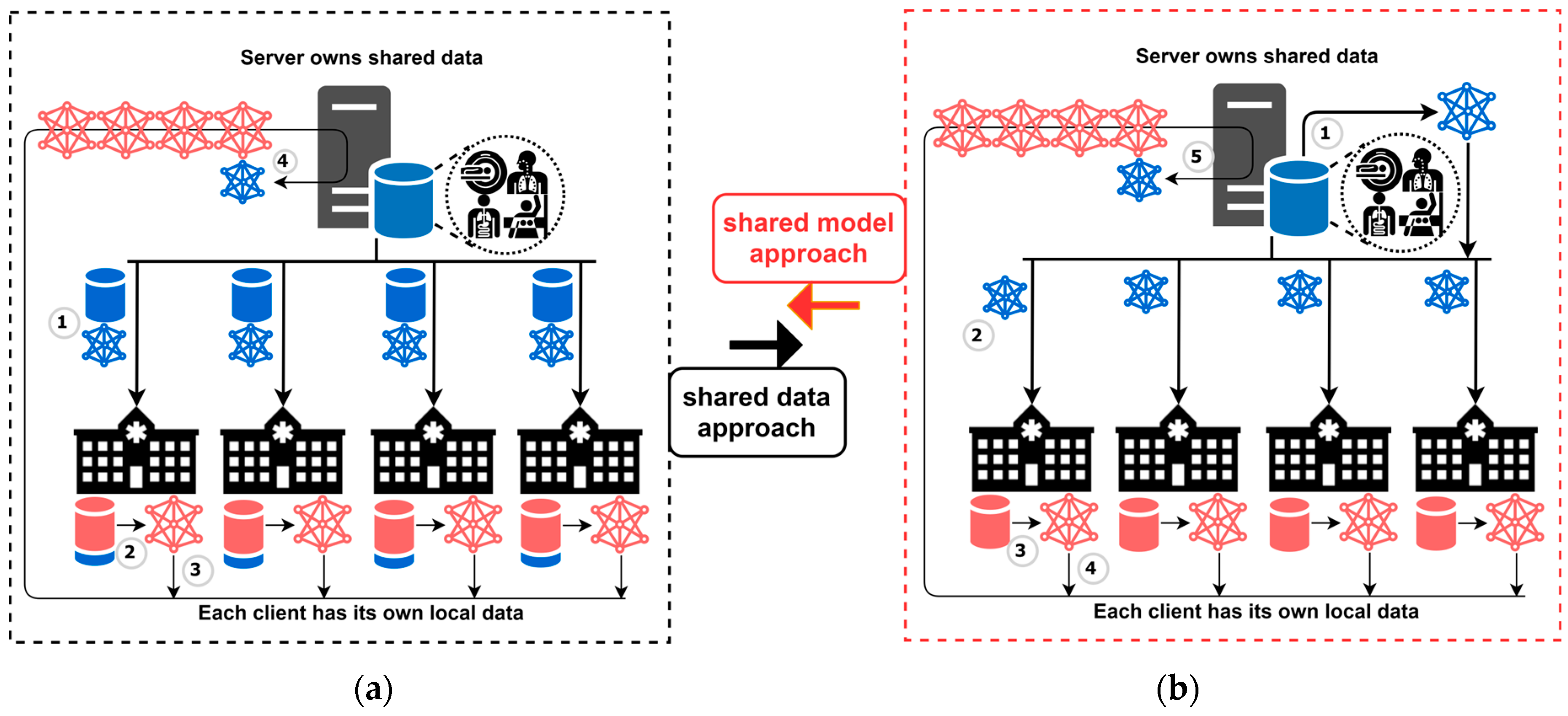
Zhao et al. [
18] proposed a shared data approach, and the training process is illustrated in
Figure 2a. Their work assumes that a portion of shared data resides on the server side. When the training process starts, each institution trains a local model with the shared data from the server and the local data residing on the institution side. In this way, institutions can expand their data to increase the amount of training data and alleviate the Non-IID problem. To this end, when an institution has only one data label, an expansion of the dataset on the server has all data labels. While applying the shared data scheme, each institution can access all the data from the server. Therefore, data expansion is beneficial for local training, and the server eventually aggregates a more efficient global model through the local models. However, transmitting the dataset violates the principle of avoiding raw data exchange in FL and also imposes additional burdens on the network.
In view of this, this paper proposes a shared model approach inspired by the concept of the shared data approach. This paper applies the concept of a pre-trained model with a shared model to achieve more efficient optimization. The training process of our proposed method is shown in
Figure 2b. In the shared model approach, the network traffic during the training process can be reduced because shared data does not need to be exchanged in FL. Moreover, the training process is further modified using the FedProx approach [
7] to simplify model gradient updates. Each institution trains its local model and aggregates the model before and after the local training. In the server, all local models, along with the previous round of global models, are collected for aggregation. Hence, the model gradient is updated by a small magnitude, as per the shared model. The detailed training processes are described as follows.
Initially, the server owns the shared data. In each round of training, the server first trains a global model using the shared data to obtain a shared model;
After training the shared model, the server sends the shared model as a global model to each institution;
Each institution performs local training to generate a local model, which is then aggregated with the global model;
Each institution sends its local model back to the server for aggregation;
The server aggregates local models from all institutions from the previous round of the global model.
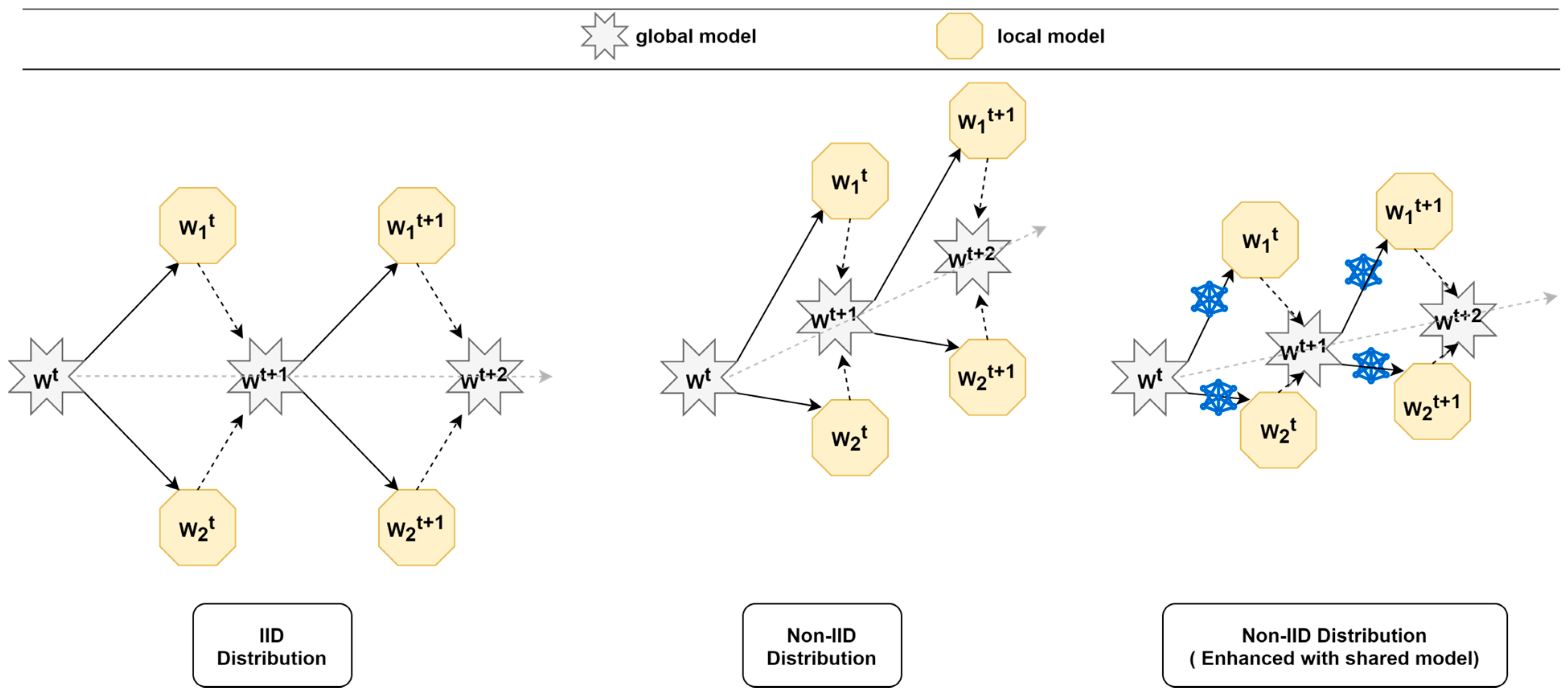
The model update profile shown in
Figure 3 highlights the significant differences that can arise for FL training when dealing with IID and Non-IID data distributions. In the case of IID, each institution has the same data distribution and data quantity, making it easy to find the global optimum during aggregation because the local update process of each institution does not differ too much. However, in the case of Non-IID data distribution, it is easy to get stuck in a local optimum because the data distribution and quantity of data in each institution are different. Some features can only be learned by specific institutions but can be forgotten due to different data distributions, leading to a decrease in FL model efficiency. Through the shared model, institutions can continue training based on the shared model and modify the algorithm to slow down the update process, resulting in better aggregation results for the global model.
The experiments presented in
Section 4.1 demonstrate that the proposed algorithm effectively updates the shared model towards global optimization. The novel approach is able to achieve good performance even with a smaller portion of the whole dataset and even when institutions face the catastrophic forgetting problem after local training. The results indicate that using a shared model can improve accuracy in cases of an extremely imbalanced data distribution. With only 5% of shared data used for training, a 25% improvement in accuracy can be obtained. Higher accuracy can be achieved when more shared data are used to train the shared model.
However, training the shared model with shared data on the server may not be feasible in a practical medical scenario. Moreover, sharing data is difficult to achieve due to data sensitivity. These datasets may only be used for scientific research purposes and may not be openly accessible. In the next subsection, a CSM is proposed among institutions to find an alternative solution and replace the ideal shared data.
3.2. Candidate Selection Mechanism (CSM)
To address privacy concerns, this paper proposes a Candidate Selection Mechanism (CSM) to train a shared model using data from the best candidate institution. The assessment factor used in the CSM is initially determined by the sample size of the dataset and the number of labels at the local institution. Let
|L| denote the total number of labels and
Li denote the number of labels at a particular institution
i. Let
S denote the total data quantity across all institutions and
Si denote the quantity of data at a particular institution
i. The preliminary score is defined by the parameter
β, which weighs the different factors. When
β is smaller, the institution with more data has a higher score. When
β is larger, the institution with more data labels has a higher score. Hence, the preliminary score (
PScore) is calculated as follows.
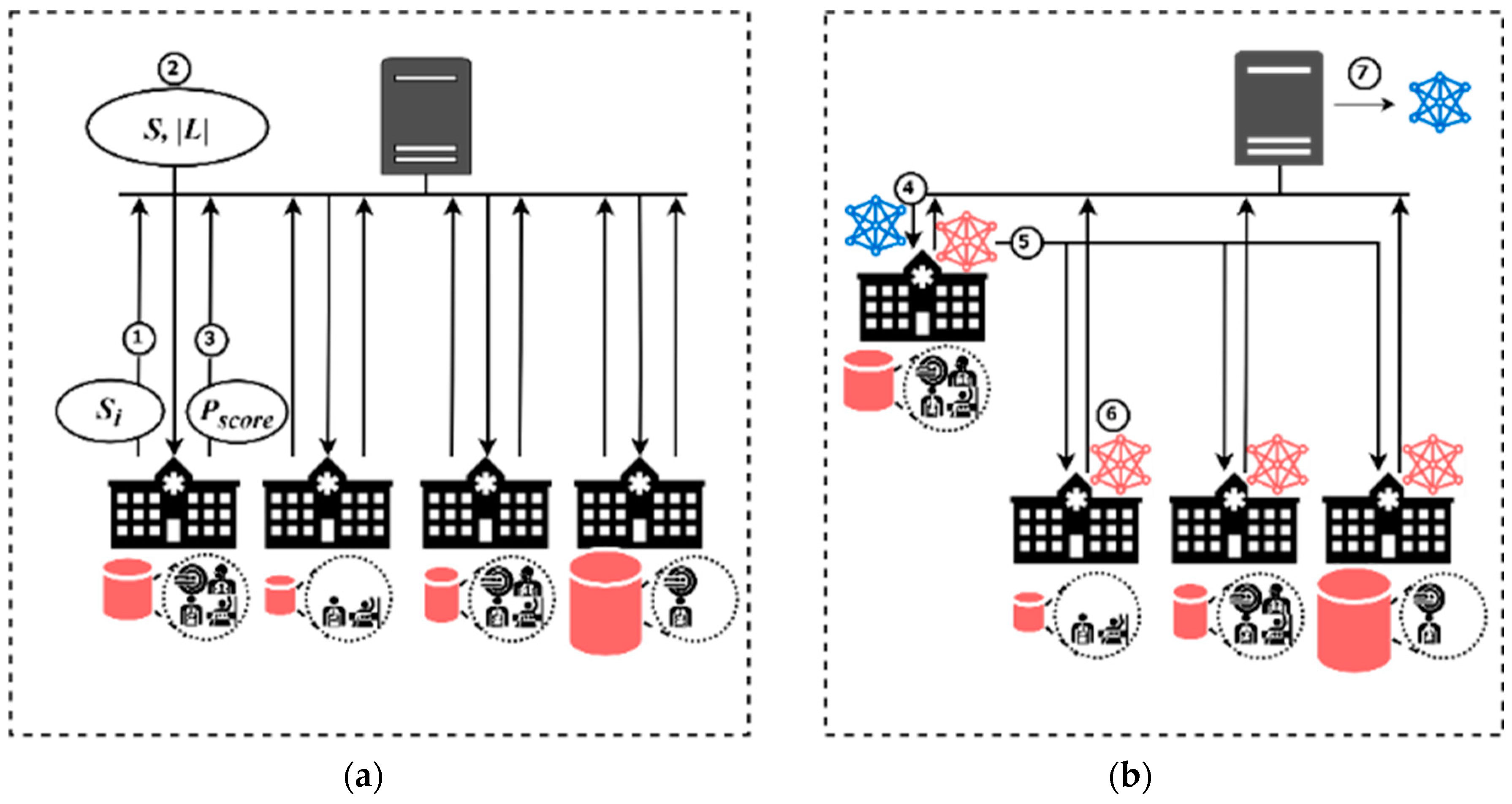
Figure 4 illustrates how the CSM can be used to select an appropriate institution for training the shared model. In the initialization process, as shown in
Figure 4a, the server collects the data quantity (
Si) from all the institutions. Next, the total data quantity (
S) and the total number of data labels (
|L|) are transmitted to each institution. Each institution calculates the assessment score according to Equation (4), which is initially determined by the sample size of the dataset and the number of labels residing locally. Once each institution calculates its assessment score, it sends the score to the server. In the candidate and training process, as shown in
Figure 4b, the server notifies the institution with the highest assessment score to start the training first. The institution with the highest
Pscore sends its local model to the remaining institutions. The remaining training process is the same as the training process in the shared model, as shown in Step 3~5 of
Figure 2b. In this way, the CSM replaces the shared data collection, and the workload of the server can also be reduced while maintaining data privacy.
Section 4.2 presents detailed experiments that reveal that the accuracy of institutions is not proportional to their data quantity when an imbalanced data distribution occurs. Instead, institutions with complete data labels perform better. However, this experiment was only conducted on a small scale and did not consider remaining exceptions, such as imbalanced data distribution causing the Non-IID problem. The next subsection introduces more advanced factors that can be applied in the CSM to address this issue.
3.3. Balanced CSM
Since the CSM considers only monotonic factors, the impact scores for institutions cannot be accurately assessed. Therefore, a Balanced Candidate Selection Mechanism (Balanced CSM) was proposed to consider more advanced factors in assessing the data of an institution. Imbalanced data distribution has been shown to result in performance degradation [
46]. Inconsistent sample size makes it difficult for the model to learn complete features. The data used to train the shared model in each institution should satisfy two conditions: (i) having more data labels and (ii) having more balanced data. The shared model is trained using the Balanced CSM to identify the institution with the most balanced data, leading to better performance for the shared model.
In this regard, label completeness should be considered a significant impact factor in accuracy performance. Let
Si,l denote the data quantity of each label
l in institution
i. The sample size of each label in the institution is converted using
Li. The converted score,
Ci, is closer to the sum of the sample size when the institution has more complete labels. In other words, the score is calculated based on label completeness before summation. The institution that has more data labels reduces the score loss for conversion. Thus, the equation is calculated using Equation (5).
Furthermore, the assessment score for each institution eventually considers the following critical factors:
Label completeness and data quantity. As shown in Equation (5), the score of data quantity is constrained by label completeness. The number of data labels at an institution determines its score for data quantity, as training a shared model requires relatively complete data and vice versa. If an institution has fewer data labels, its score for data quantity will be lower;
Local and overall standard deviation. The standard deviation indicates the degree of data imbalance. The more imbalanced the data distribution is, the larger the standard deviation becomes. Both local standard deviation (σi) and overall standard deviation (σall) are used to evaluate the factor of data distribution imbalance. When training the shared model with the same amount of data, it is preferable for the data distribution to be relatively balanced. The score is decreased if σi is larger than σall and vice versa;
Minimum sample size. Sparse sample size may result in inaccurate assessments. Equation (6) considers label completeness, but it does not account for the minimum sample size, represented by min (Si,l). In cases with sparse samples of labels, more scores are preserved during the conversion operation if there are more non-zero samples. Similarly, the standard deviation does not consider the average of the total sample size, which means that data distributions with high and low average sample sizes may have the same standard deviation. To address these limitations, min (Si,l) is needed as a factor in the assessment. When the min (Si,l) in an institution is more sparse, the score is lower and vice versa.
Therefore, each institution
i considers these factors to calculate an expected score,
Ei, according to Equation (6), and then it sends the result back to the server. The server selects the institution with the highest score as the candidate for training the shared model.
The shared model with Balanced CSM is incorporated into the FedISM algorithm (as shown in Algorithm 1), assuming that there are a total of I institutions participating in a round of training. All sets of labels are denoted as L, and the sum of all the sample sizes is denoted as S. Each institution i has a set of data labels denoted as Li, and the sample sizes are denoted as Si. The initialized procedures are presented in lines 2 to 9. First, the server initializes each institution i and obtains all label sets for the training process. After initialization, each institution i calculates its data quantity Si and standard deviation σi and sends them to the server. The server calculates the sum of Si to obtain S and the average of σi to obtain σall. After calculating S and σall, the server sends them to each institution. All institutions compute their expected scores Ei based on Equations (5) and (6) and send the score back to the server. The server selects the institution with the highest score as the candidate institution for training the shared model.
The candidate selection procedures are presented in lines 10 to 16. After receiving Ei, the server groups the institutions into normal and candidate sets. The institution with the highest Ei is designated as icandidate, and the remaining institutions are grouped in inormal. The icandidate represents the institution that has the most balanced data distribution and is responsible for training the shared model. The training procedures are presented in lines 17 to 24. In each round of training, the icandidate first performs LocalTraining() to obtain the local model. The local model trained by icandidate is taken as the global model and sent to institutions inormal that have not yet been trained. Each icandidate starts the LocalTraining() to get the local model and sends it to the server. After the server receives all the local models, the local model of each institution is aggregated with the previous round of the global model to obtain a new global model. In the next round, the global model is trained continuously by the same icandidate until the completion of the training rounds.
| Algorithm 1: FedISM |
| | Input: all institutions , communication rounds , local epochs , learning rate |
| | Output: The final model |
| 1 | Server executes: |
| 2 | | initial each institution |
| 3 | | Get all set of labels |
| 4 | | Get data quantity and standard deviation from institutions |
| 5 | | |
| 6 | | |
| 7 | | for each institution do |
| 8 | | | ExpectedScore) |
| 9 | | end for |
| 10 | | for each institution do |
| 11 | | | if ) then |
| 12 | | | | = |
| 13 | | | else |
| 14 | | | | .append |
| 15 | | | end if |
| 16 | | end for |
| 17 | | for round do |
| 18 | | | executes LocalTraining) and get local model |
| 19 | | | send the local model to every |
| 20 | | | for do |
| 21 | | | | LocalTraining |
| 22 | | | end for |
| 23 | | | |
| 24 | | end for |
| 25 | | return |
| 26 | ExpectedScore): |
| 27 | | Calculate based on Equation (3) |
| 28 | | |
| 29 | | Calculate based on Equation (4) |
| 30 | | return |
| 31 | LocalTraining: |
| 32 | | |
| 33 | | for epoch do |
| 34 | | | for each batch of local data do |
| 35 | | | | |
| 36 | | | |
| 37 | | return to the server |
To analyze the complexity of the FL algorithm, assuming that
T represents the communication round,
I represents the number of institutions, and
L represents the time of local training. Therefore, the time complexity of traditional FedAvg is represented by Equation (7).
In FedISM, due to assessments of the completeness of a dataset, each institution calculates its own assessment score before the training process. Then, the server needs to select the institution with the highest score to prioritize the training of the shared model, followed by the other institutions. Therefore, the time complexity of FedISM is represented by Equation (8), where
E represents the time to calculate the assessment score.
The time complexity of FedISM is slightly higher than that of FedAvg because FedISM requires an initialization process to calculate the scores. However, these differences are small because the calculation time of I × E + I is far less than T and L. Thus, the additional calculations can be ignored. The time complexity of FedISM approximates O (T × L × I).
4. Performance Evaluations
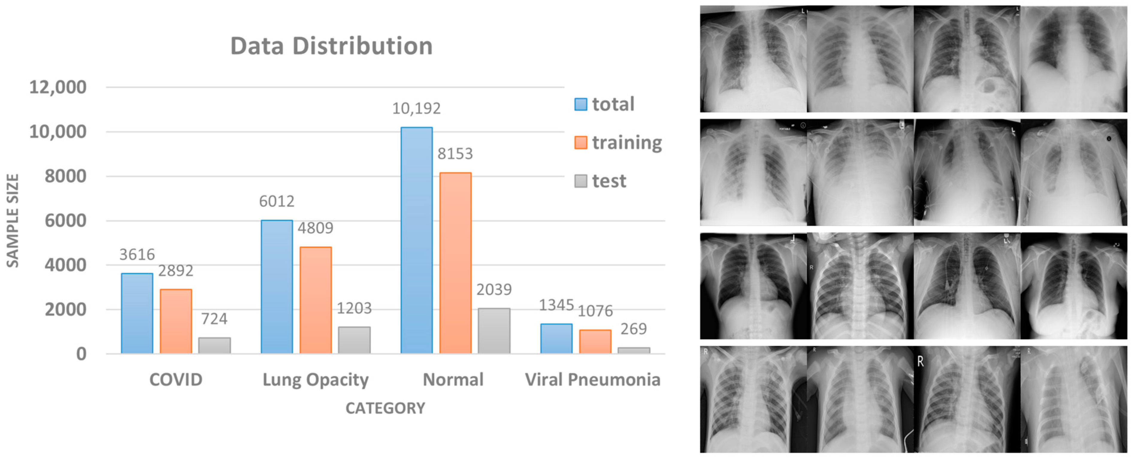
In practical medical scenarios, the classification problem often involves multiple classes rather than a purely binary classification. Therefore, the COVID Radiography Database [
47,
48] was used as our dataset to demonstrate the medical data in this paper. The dataset contains a total of 21,165 X-ray images, which are divided into four categories: COVID, lung opacity, normal, and viral pneumonia. The data distribution and some sample images are shown in
Figure 5. The dataset is a compilation of publicly accessible databases, such as Chest X-Ray (CXR) [
1] and Pneumonia [
49]. Using this dataset provides developers with a variety of data to adapt the classification model.
For data pre-processing, the experiments take 80% of the dataset for each label as the training data and the remaining 20% as the test data. The DNN model applied in the experiments was the ResNet18 neural network [
50], and the optimizer was SGD. The setting for weight_decay was 1 × 10
−4, and the learning rate was adjusted to 1 × 10
−3. CrossEntropyLoss was used as the loss function. The rest of the experimental configurations and data distributions are described in each subsection.
4.1. Shared Model Experiments
This paper proposes the concept of a shared model to alleviate the challenge of data imbalance without exchanging shared data. In this experiment, the number of institutions was set to four, which corresponds to the number of data labels. The data allocation principle first assigns the shared data according to the experiment ratio, while the rest of the data are private and assigned to different Non-IID configurations. In our experiments, the ratios of shared data were set at 5%, 10%, and 15% for evaluations. The private data were divided into Non-IID (1), Non-IID (2), Non-IID (3), and Non-IID (4), where Non-IID (n) represents the number of data labels owned by each institution. For example, Non-IID (1) means that each institution has only one label for its private data, while Non-IID (4) means that the sample sizes and data labels of the private data are equally distributed among all institutions. The simulation parameters were set to 100 rounds, 5 local epochs for FL, and 100 epochs for CL.
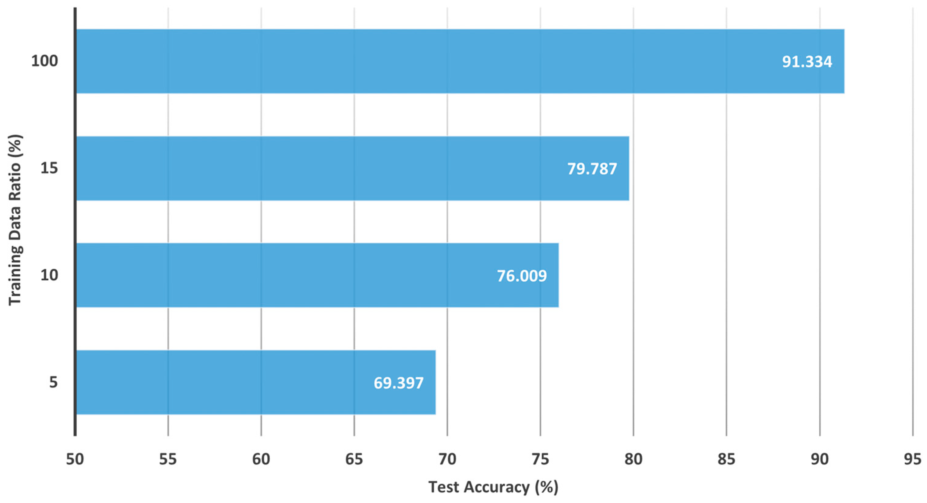
Figure 6 and
Table 2 demonstrate the effectiveness of the shared model in different Non-IID distributions when compared to FedAvg and CL. The experimental results for CL are depicted in
Figure 6, where the accuracy could achieve 69%, 76%, 79%, and 91% when the training data were applied at 5%, 10%, 15%, and 100%, respectively. Training with a smaller sample size results in a model that is unable to learn features completely. On the other hand, the effectiveness of the shared model with FedAvg is depicted in
Table 2, where FedAvg and the shared model were trained using 5%, 10%, and 15% of the shared data in the case of Non-IID distributions. Experimental results show that the test accuracy of FedAvg was close to 90% in Non-IID (4). However, the accuracy decreased when the institutions had fewer labels. The accuracy dropped to 89%, 74%, and 52% in Non-IID (3), Non-IID (2), and Non-IID (1), respectively. When the degree of Non-IID was more severe, the local model learned more inconsistent features. The Non-IID problem dramatically decreases the performance in FL.
Table 2 also records the convergence time for each method to achieve a specified test accuracy of 80%. The results show that Non-IID has a significant impact on FedAvg under different data distributions. FedAvg could not reach the specified test accuracy within 100 rounds in some cases, such as Non-IID (1) and Non-IID (2) distributions. In the Non-IID (1) distribution, FedAvg performance was only 51.688%, making convergence impossible. Through the use of a shared model, convergence time could be effectively improved, which is particularly evident in Non-IID (1). Moreover, the convergence speed increased with the amount of data used to train the shared model.
This experiment yielded several important findings. The first is that the shared model trained by the shared data generally improved performance across different data distributions. In particular, the shared model was effective in addressing high-skew distributions with Non-IID (1) and Non-IID (2) configurations. For example, with a minimum of 5% shared data, the shared model improved the accuracy of Non-IID (1) and Non-IID (2) by 25% and 8%, respectively, compared to FedAvg. Although the performance improvements for Non-IID (3) and Non-IID (4) were less pronounced, the performance of the shared model was also comparable to that of CL when trained on 100% of the data. Notably, a 5% sharing model provided the largest performance improvement, while higher sharing rates (10% or more) tended to produce further improvements and be more stable.
Another notable finding from this experiment is the relationship between the effectiveness of the shared model and FL performance. The shared model could further improve the performance of FL. For example, when training with highly skewed Non-IID (1) using FedAvg, the accuracy was only 51%, while CL achieved 69% accuracy with 5% shared data. However, when training with a 5% shared model, the accuracy of Non-IID (1) was improved to 76%. Furthermore, if the shared model is properly trained, the aggregated model can move towards global optimization. Although institutions may still have a catastrophic forgetting problem after local training, the shared model could be a breakthrough for FL because applying 5% of shared data can significantly enhance test accuracy.
Obviously, training the shared model with shared data can achieve a significant effect. However, this assumption of existing shared data is unreasonable due to the importance of privacy issues in FL, which are magnified and examined in medical scenarios. Therefore, a CSM mechanism is desired to replace the shared data approach. In addition, experiments using highly skewed data distributions are conducted in this section and are suitable for face recognition applications [
51]. Hence, alternative methods are needed to simulate various data distributions without sacrificing experimental completeness and matching reality.
4.2. CSM Experiments
The proposed CSM method enables training of the shared model without relying on the shared data stored on the server. Instead, CSM attempts to identify an institution whose data are representative of all participating institutions. The shared model is then trained using the data from this selected institution rather than the shared data. Since CSM cannot directly access the raw data from each institution, the selection process relies on accessing the metadata to make informed decisions.
While respecting data privacy constraints, the CSM method utilizes an assessment score that considers various factors to represent the importance of an institution’s data. Specifically, Equation (3) calculates the assessment score using two impact factors with different weights (β = 0.2, β = 0.5, β = 0.8) to reflect the amount and quality of the data in each institution. A smaller β value means that the institution has a larger amount of data and will receive a higher score. On the contrary, a higher β value indicates that the institution has a higher proportion of data labels and will also receive a higher score. The institution with the highest score is then selected as the candidate to train the shared model.
To account for various factors present in medical scenarios, such as disease type, sample size, and geographical location, the Dirichlet process [
52] was employed to simulate probability distributions. The Dirichlet process is a conjugate prior distribution for multiple distributions, and the probability parameter
α is adjusted to control the degree of data imbalance. The Dirichlet distribution is commonly used in the Bayesian generative process for data reconstruction. This process involves defining a prior distribution and specifying the hyperparameter
α, where
α represents the concentration parameter. Subsequently, random sampling from the distribution is performed based on
α to satisfy the concentration parameter. When the value of
α is small, the data distribution is more imbalanced, whereas a larger
α value tends to result in a more balanced data distribution. For this experiment, the number of institutions was set to four, and the local epoch was set to five. Three different values of
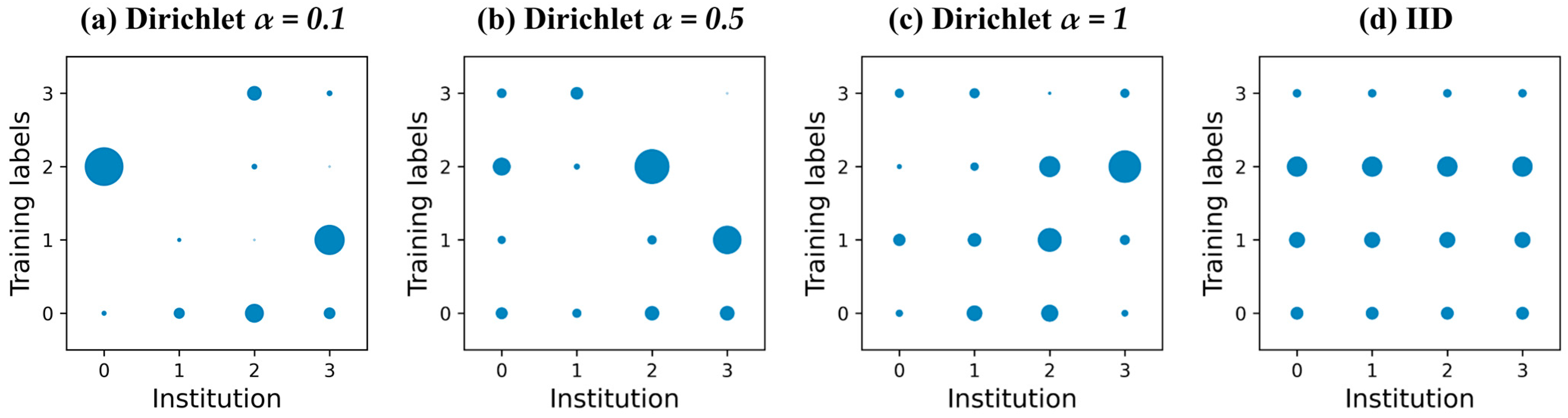
α (0.1, 0.5, and 1) and an IID scenario for balanced data distribution were used to simulate various data distribution scenarios.
Figure 7 visualizes these data distributions, from extreme imbalance to balance, moving from left to right with
α values of 0.1, 0.5, 1, and finally IID.
Table 3 presents the experimental results of CSM using different weights of
β and the FedAvg method for various data distributions. Obviously, the accuracy of each method declines as the data imbalance becomes more severe. For instance, in FedAvg, the accuracy in the IID distribution could reach 90%, which is quite close to the results of CL with 100% data. However, the accuracy gradually dropped to 64% as
α decreased, which is a 27% difference compared to CL. Among the CSM methods with different weights, CSM with
β = 0.2 tends to choose the institution with the highest data quantity while CSM with
β = 0.8 tends to select the institution with the most data labels. In a balanced data distribution, the CSM methods with different weights may pick the same institution and yield the same results.
Regarding the convergence time to achieve 85% test accuracy, FedAvg required more time to converge in various data distributions. Even FedAvg could not reach the specified test accuracy within 100 rounds in some cases. In contrast, the CSM method with β = 0.8 achieved a faster convergence time compared to other FL methods. In addition, the convergence speed was faster as α increases. Therefore, using the CSM method with β = 0.8 can lead to better convergence results in the same amount of time and improve efficiency.
In this experiment, not all institutions selected by CSM were better for training the shared model with the same performance. Specifically, the CSM with β = 0.2 performed worse than FedAvg in the imbalanced data distribution because data quantity is not dominant. For example, in the case of α = 0.1, Institution 0 had the highest data quantity, but most of the data were concentrated in the normal category, with only a small amount of data in the COVID-19 category. As a result, catastrophic forgetting of the model occurred during shared model training with imbalanced categories, leading to poorer training results.
On the other hand, the highest accuracy was achieved at CSM with β = 0.8. That is because the institution with more data labels achieved data balance, thereby eliminating the need for shared data and resulting in better training results for the shared model. However, the factors used in CSM are too simple, and none of these factors could sufficiently represent performance metrics. Thus, more advanced factors are required to assess the institutional data for further training of the shared model.
4.3. Balanced CSM Experiments
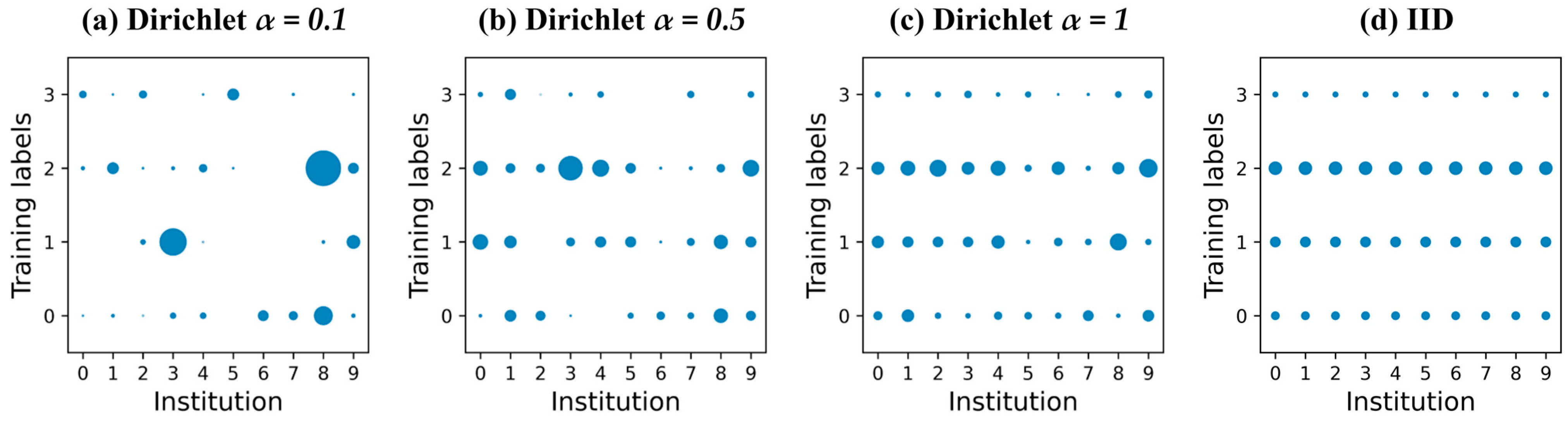
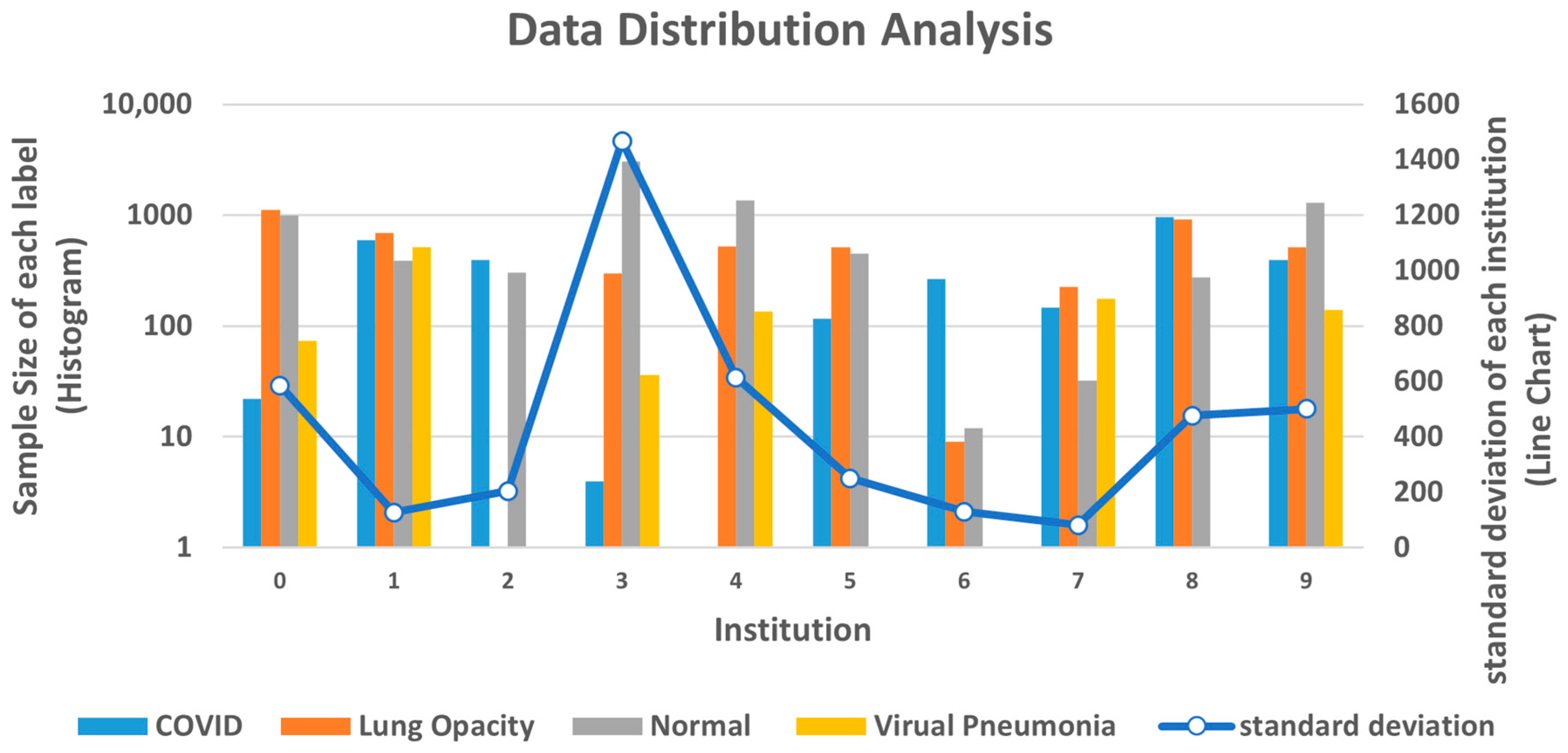
In order to improve the assessment process when there are more institutions involved, an extended version of CSM called Balanced CSM was developed. Balanced CSM incorporates additional impact factors to assess the best institution choice more accurately. These factors include label completeness and data quantity, local and overall standard deviation, and the minimum sample size. To test the effectiveness of Balanced CSM, the number of institutions in the experiment was increased to 10, with 100 rounds and 5 local epochs for FL. Dirichlet process with parameters
α = 0.1,
α = 0.5, and
α = 1 was used to simulate different data distributions, and IID was used for balanced data distribution. The different data distributions are visualized in
Figure 8.
Table 4 presents the experimental results. Similarly, the performance of FedAvg deteriorated as the data distribution became more imbalanced. In the IID case, FedAvg achieved an accuracy of 89%, which is only 2% worse than CL. However, in the case of imbalanced data distribution (
α = 0.1), the accuracy of FedAvg was only 76%, which increases the gap with CL to 15%. The factors in CSM with
β = 0.8 were not highly correlated with the data distribution, indicating that the data imbalance problem was prevalent in large scale institutions. Regarding the convergence time to achieve 75% test accuracy, CSM with
β = 0.8 could not achieve the best solution. In the data distribution with
α = 0.5, the convergence time was longer than any other method. However, in the improved Balanced CSM method, the selection mechanism was optimized to identify the best suitable institution for training so as to achieve better accuracy and convergence time.
Accordingly, the experimental results show that the accuracy of CSM with β = 0.8 was even worse than that of FedAvg at Dirichlet process with α = 0.5 or α = 1. In contrast, the accuracy of Balanced CSM was higher than the other methods. Balanced CSM utilizes three factors to identify the institution with the most balanced data, making it more effective in assessing the data for further training of the shared model.
In
Figure 9, the data distribution is shown for the Dirichlet process with
α = 0.5. Among all institutions, Institution 3 had the highest data quantity and all kinds of data labels. However, in this scenario, CSM with
β = 0.8 selected Institution 3 to train the shared model, while the Balanced CSM selected Institution 1. Even though Institution 1 did not have the highest data quantity, it had the most balanced data among all institutions. In contrast, Institution 3 had a serious data imbalance problem and the highest standard deviation among all institutions. The large difference between the highest and lowest data quantities was 700 times, which led to an imbalance problem in the training process and resulted in low accuracy performance.
Table 5 shows the results of all institutions trained with the shared model in each distribution. Evaluation metrics use accuracy, recall, precision, and F1-score to assess different aspects of the inspection. The
N-class classification (weighted average) was calculated as in Equations (9)–(12).
The results show that the institution selected by Balanced CSM had the best accuracy and higher performance in precision, recall, and F1-score. This means that Balanced CSM can improve learning in all categories and reduce the number of false positive and false negative cases. These factors in Balanced CSM extend the indicators of data quantity and label size, proving that Balanced CSM is more suitable for assessing institution data through experiments.
Overall, the factor in Balanced CSM aims to achieve a balanced characteristic. A balanced data distribution enables the model to learn the features of each label fairly. However, in an imbalanced data distribution, each institution trains a model with different training characteristics. As a result, Balanced CSM can find the most balanced data as a candidate to train the shared model. The shared model with the Balanced CSM can improve the accuracy of data distribution from imbalanced to balanced, particularly when the data is extremely imbalanced.
5. Conclusions and Future Works
Data imbalance is a common challenge in FL that has not been fully alleviated in previous works. This paper aimed to address this challenge by proposing the FedISM approach for COVID-19 detection. This scenario is more suitable for practical medical applications where raw data cannot be exchanged between medical institutions. By applying FedISM, data privacy and data imbalance problems between institutions can be alleviated. There are two main contributions of FedISM that increase feasibility in a practical medical scenario. First, the shared model approach enhances the shared data approach by not exchanging raw data during the training process, while also modifying the algorithm to achieve higher accuracy with smaller gradient updates. Second, while shared data is ideal, it is not practical for FL applications. Instead, the shared model can be trained by the institution as an alternative way. To achieve this, a CSM was proposed to calculate an assessment score for the dataset of each institution.
The experimental results show that FedISM can efficiently alleviate data imbalance issue by identifying the most suitable institution for training the shared model. A significant improvement was achieved when training the shared model using only 5% of the shared data. In the highly skewed distribution of Non-IID (1), FedISM improved accuracy by 25% compared to FedAvg. The shared model improves the aggregation effect and can be trained without sharing raw data. The CSM evaluates the most balanced data distribution based on several key factors to train the shared model. The Dirichlet process is used to simulate various data distributions and compare performance evaluations between the IID and Non-IID scenarios. Results indicate that Balanced CSM can further enhance accuracy by 6% in highly imbalanced data distributions.
To summarize, this paper discussed the impacts of data imbalance on test accuracy and convergence time in FL. Some issues, such as secure transmission, heterogeneous clients, and noise data during FL training, were not considered in this paper. These issues may require further investigation to gain a more comprehensive understanding. The mobility of participating clients is also interesting, and FL could potentially be combined with Internet of Vehicles (IoV) scenarios, which may encounter various issues such as communication costs and convergence time among dynamic joining/leaving clients.
In future work, three directions are planned to move forward. First, developing a framework for practical deployments of distributed FL is critical. The Taiwan AI lab has already developed a simple project using Kubernetes. The leverage of the open-source project and our work could be feasible. Second, moving towards a decentralized FL framework is also an important area for future work. Last but not least, considering factors such as late joiners or offline participants that occur in practical scenarios may bring another challenge to FL. Addressing these challenges of deploying FL in practical scenarios is also a potential topic for further research.


