
Chaotic Sand Cat Swarm Optimization

Abstract
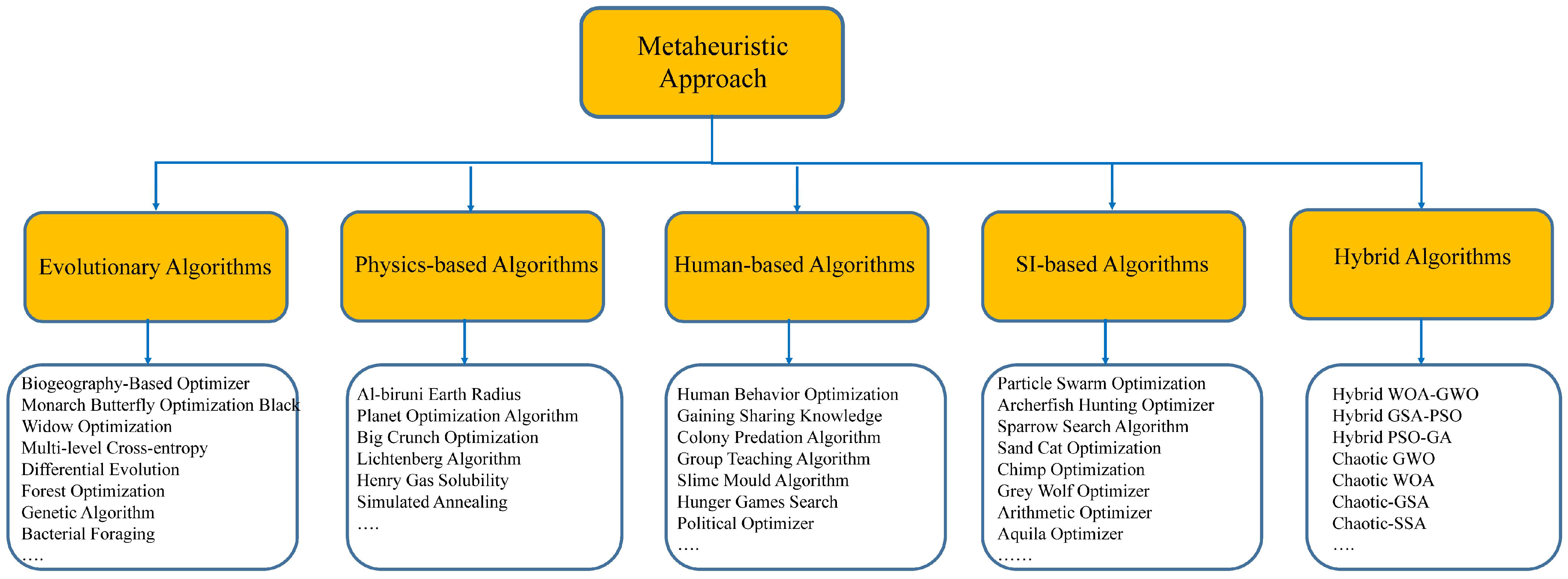
:1. Introduction
- (1)
- It is to integrate the chaos feature of non-recurring locations into SCSO’s core search process to improve global search performance.
- (2)
- The problem of slow transitions between phases and early or late convergence is decreased.
- (3)
- It focuses on exploration as early as possible to avoid falling into local optimization.
- (4)
- It tries to find the best or near−optimum solutions by increasing the probability of the population spread.
- (5)
- By using 12 different maps, the most suitable map for SCSO is determined. Therefore, it is a chaos-based inclusive algorithm for SCSO.
- (6)
- The method is flexible and can be easily adapted to different types of optimization problems.
2. Related Works
3. Overview of Sand Cat Swarm Optimization
| Algorithm 1. Standard SCSO pseudocode |
| Initialize the population. Calculate the fitness function based on the objective function. Obtain a random angle. Initialize the c, R, r based on the Equations (2)–(4) While (t <= maximum iteration) For each search agent If(abs(R) <= 1) Update the search agent position based on the Equation (5a). Else Update the search agent position based on the Equation (5b). End End t = t++ End |
4. CSCSO: Chaotic Sand Cat Swarm Optimization Algorithm
| Algorithm 2. Pseudocode of proposed CSCSO |
| Initialize the population. Calculate the fitness function based on the objective function to find the best search agent: Xbest. Obtain a random angle. Initialize p. Initialize the r, c, and R. Initialize the value of the chaotic map. While (t <= Max_Iteration) Update the chaotic value using the respective chaotic map. For each sand cat (search agent) If (p < 0.5) Update the search agent position based on the Equation (5) Else Update the search agent position based on the Equation (10). End If Update r, R, and p. End for Check if any search agent goes beyond the search space and amend it. Calculate the fitness of each search agent. Update Xbest if there is a better solution. t = t++ End while return Xbest. |
5. Simulation Experiments
5.1. Experiments’ Settings
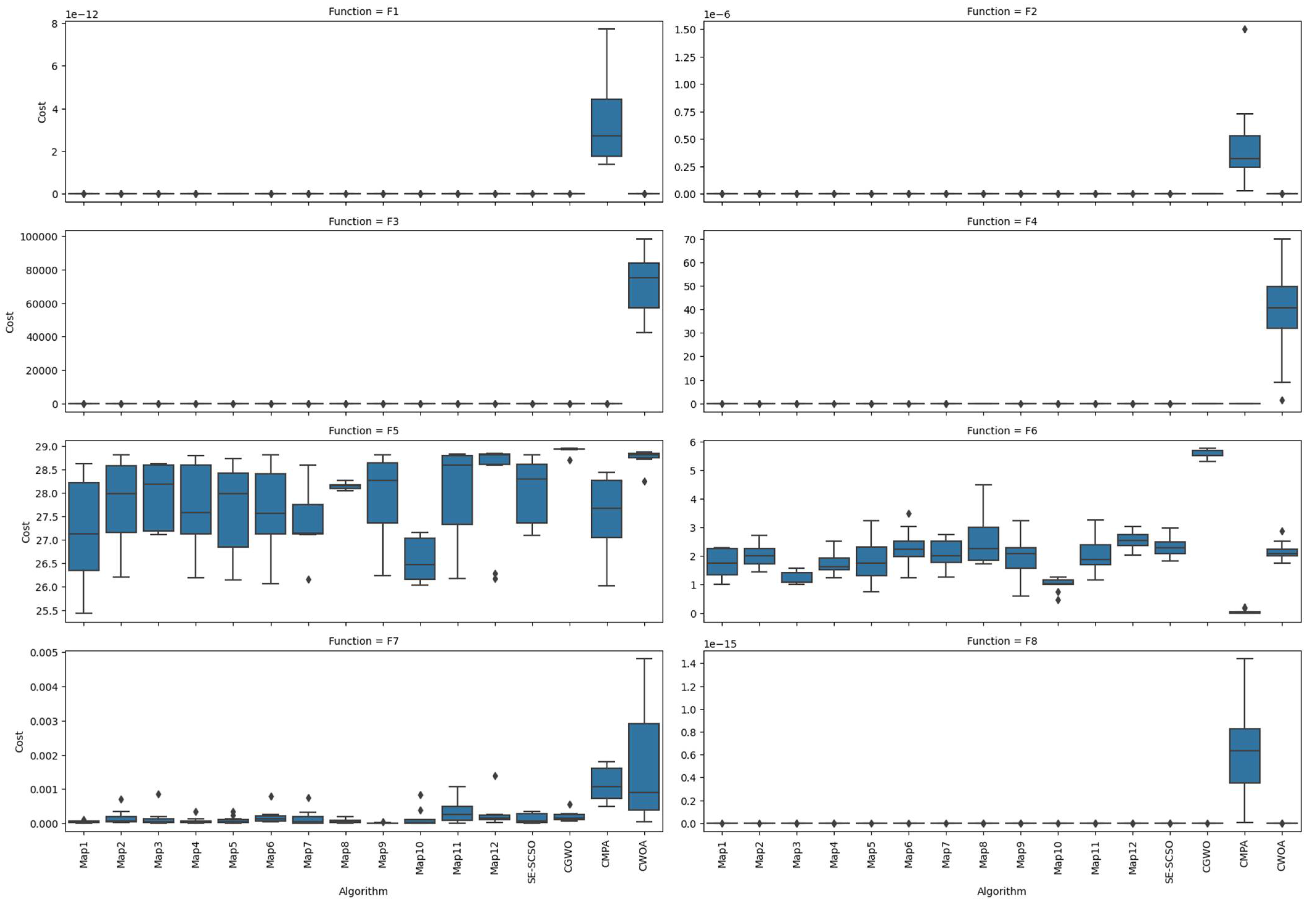
5.2. Results and Discussion in Unimodal Test Functions
- 1-Analysis of the proposed algorithm within itself and between the maps used
- 2-Comparison and analysis of the proposed algorithm with the SE-SCSO
- 3-Comparison and analysis of CSCSO algorithm with other three chaotic-based algorithms
5.3. Results and Discussion in Multimodal Test Functions
- 1-Analysis of the proposed algorithm within itself and between the maps used.
- 2-Comparison and analysis of the proposed algorithm with the SE-SCSO
- 3-Comparison and analysis of CSCSO algorithm with other three chaos-based algorithms
5.4. Results and Discussion in Competitive Test Functions
5.5. Results and Discussion in Numerical Real-World Optimization Problems
5.6. Local Optima and Convergence Curve
5.7. Diversity Analysis
5.8. Exploration and Exploitation Analysis
6. CSCSO in Constrained Engineering Problems
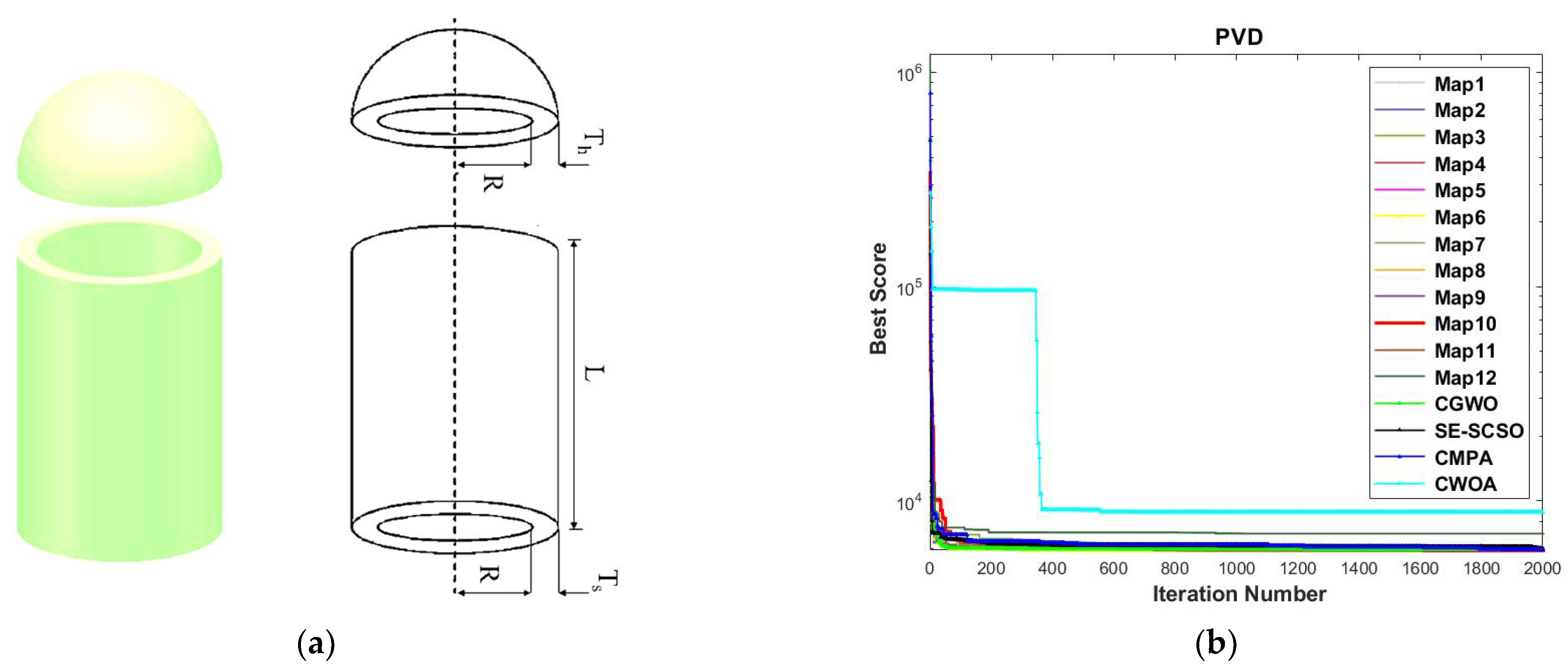
6.1. Results and Discussion in Pressure Vessel Design Problem
6.2. Gear Train Design Problem
6.3. Tension/Compression Spring Design Problem
6.4. Speed-Reducer Design Problem
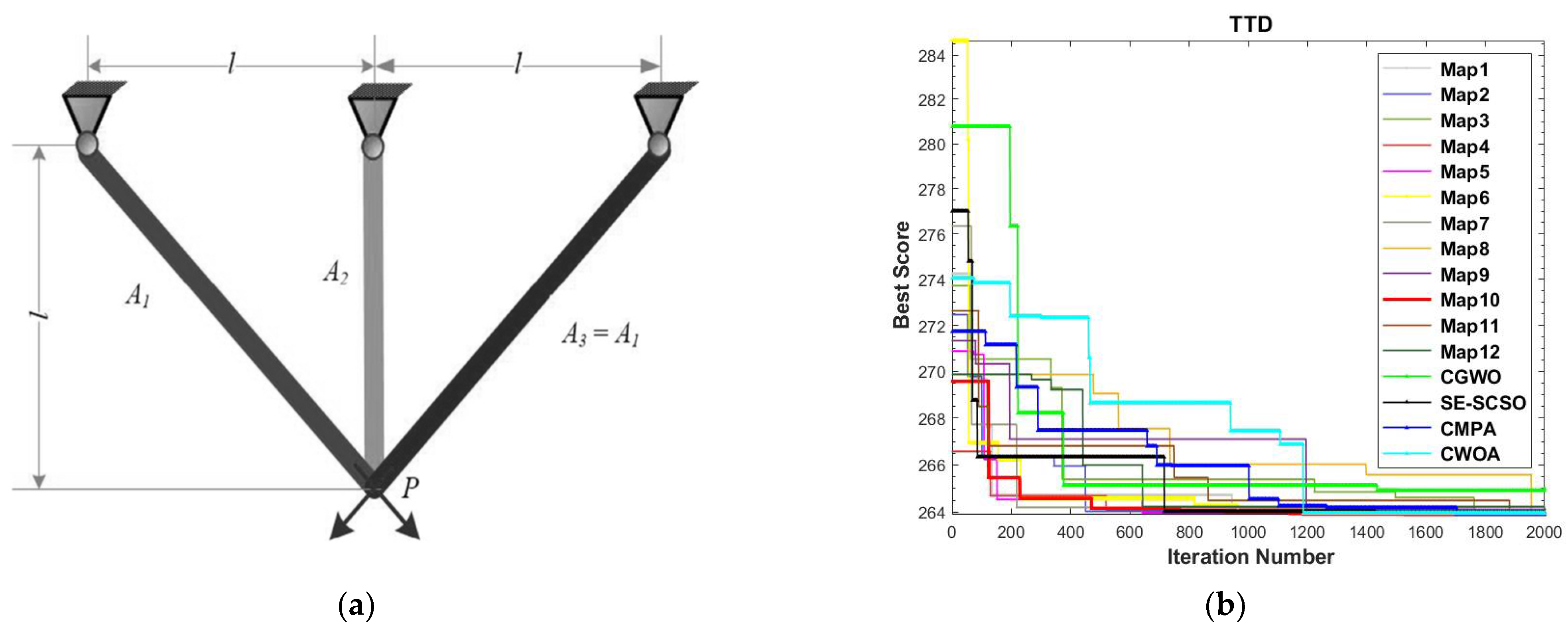
6.5. Three-Bar Truss Design Problem
7. CSCSO in Constrained Social Sciences-Based Problems
8. Conclusions
Author Contributions
Funding
Institutional Review Board Statement
Informed Consent Statement
Data Availability Statement
Acknowledgments
Conflicts of Interest
Appendix A

| Formula | Dim | Range | Global Minimum |
|---|---|---|---|
| 30 | [−100, 100] | 0 | |
| 30 | [−10, 10] | 0 | |
| 30 | [−100, 100] | 0 | |
| 30 | [−100, 100] | 0 | |
| 30 | [−30, 30] | 0 | |
| 30 | [−100, 100] | 0 | |
| 30 | [−1.28, 1.28] | 0 | |
| 30 | [−100, 100] | 0 |
| Formula | Dim | Range | Global Minimum |
|---|---|---|---|
| 30 | [−500, 500] | −418.9829 × dim | |
| 50 | [−100, 100] | 0 | |
| 30 | [−50, 50] | 0 | |
| 30 | [−50, 50] | 0 | |
| 50 | [−5.12, 5.12] | 0 | |
| 50 | [−10, 10] | 0.9 | |
| 50 | [−500, 500] | 0 | |
| 50 | [−10, 10] | −1 |
| Function | Benchmark Function | Dim | Range | |
|---|---|---|---|---|
| CEC01 | Storn’s Chebyshev Polynomial Fitting Problem | 9 | [−8192, 8192] | 1 |
| CEC02 | Inverse Hilbert Matrix Problem | 16 | [−16,384, 16,384] | 1 |
| CEC03 | Rastrigin’s Function | 10 | [−100, 100] | 1 |
| CEC04 | Grıenwank’s Function | 10 | [−100, 100] | 1 |
| CEC05 | Weiersrass Function | 10 | [−100, 100] | 1 |
| CEC06 | Modified Schwefel’s Function | 10 | [−100, 100] | 1 |
| CEC07 | Expanded Schaffer’s F6 Function | 10 | [−100, 100] | 1 |
| CEC08 | Ackley Function | 10 | [−100, 100] | 1 |
| Function | Benchmark Function | Dim | Range | |
|---|---|---|---|---|
| R1 | Shifted and Rotated Griewank’s Function without Bounds | 50 | [−600, 600] | 700 |
| R2 | Shifted and Rotated Rastrigin’s Function | 50 | [−5, 5] | 500 |
| R3 | Shifted and Rotated Weierstrass Function | 50 | [−0.5, 0.5] | 300 |
| R4 | Shifted and Rotated Expanded Scaffer’s | 50 | [−100, 100] | 600 |
| R5 | Shifted and Rotated Schwefel’s function | 10 | [−100, 100] | 1100 |
| R6 | Shifted and Rotated Lunacek bi−Rastrigin function | 10 | [−100, 100] | 700 |
| R7 | Hybrid function 2 (N = 4) | 10 | [−100, 100] | 1600 |
| R8 | Composition function 2 (N = 4) | 10 | [−100, 100] | 2400 |
| The mathematical equations of pressure vessel design problem (, ((( |
| The mathematical equations of gear train design problem |
| The mathematical equations of tension/compression spring design problem (, ( (( ( |
| The mathematical equations of speed reducer design problem |
| The mathematical equations of three-bar truss design problem |
References
- Abdel-Basset, M.; Mohamed, R.; Jameel, M.; Abouhawwash, M. Nutcracker optimizer: A novel nature-inspired metaheuristic algorithm for global optimization and engineering design problems. Knowl. Based Syst. 2023, 262, 136. [Google Scholar] [CrossRef]
- Abualigah, L.; Diabat, A.; Mirjalili, S.; Abd Elaziz, M.; Gandomi, A.H. The Arithmetic Optimization Algorithm, Computer Methods. Appl. Mech. Eng. 2021, 376, 113609. [Google Scholar] [CrossRef]
- Kiani, F.; Anka, F.A.; Erenel, F. PSCSO: Enhanced Sand Cat Swarm Optimization Inspired by the Political System to Solve Complex Problems. Adv. Eng. Softw. 2023, 178, 103423. [Google Scholar] [CrossRef]
- Kalinin, K.P.; Berloff, N.G. Computational complexity continuum within using formulation of NP problems. Nat. Commun. Phys. 2022, 5, 20. [Google Scholar]
- Kumar, S.; Yildiz, B.S.; Mehta, P.; Panagant, N.; Sait, S.M.; Mirjalili, S.; Yildiz, A.R. Chaotic marine predators algorithm for global optimization of real-world engineering problems. Knowl. Based Syst. 2023, 261, 110192. [Google Scholar] [CrossRef]
- Wolpert, D.H.; Macready, W.G. No free lunch theorems for optimization. IEEE Trans. Evol. Comput. 1997, 1, 67–82. [Google Scholar] [CrossRef]
- Kiani, F.; Seyyedabbasi, A.; Aliyev, R.; Gulle, M.U.; Basyildiz, H.; Shah, M.A. Adapted-RRT: Novel hybrid method to solve three-dimensional path planning problem using sampling and metaheuristic-based algorithms. Neural Comput. Appl. 2021, 33, 15569–15599. [Google Scholar] [CrossRef]
- Nematzadeh, S.; Torkamanian-Afshar, M.; Seyyedabbasi, A.; Kiani, F. Maximizing coverage and maintaining connectivity in WSN and decentralized IoT: An efficient metaheuristic-based method for environment-aware node deployment. Neural Comput. Appl. 2023, 33, 15569–15599. [Google Scholar] [CrossRef]
- Salgotra, R.; Singh, S.; Singh, U.; Mirjalili, S.; Gandomi, A. Marine predator inspired naked molerat algorithm for global optimization. Expert Syst. Appl. 2023, 212, 118822. [Google Scholar] [CrossRef]
- Al-Gharaibeh, R.; Ali, M. Real-parameter constrained optimization using enhanced quality-based cultural algorithm with novel influence and selection schemes. Inf. Sci. 2021, 576, 242–273. [Google Scholar] [CrossRef]
- Kiani, F.; Seyyedabbasi, A.; Nematzadeh, S.; Candan, F.; Çevik, T.; Anka, F.A.; Randazzo, G.; Lanza, S.; Muzirafuti, A. Adaptive Metaheuristic-based Methods for Autonomous Robot Path Planning: Sustainable Agricultural Applications. Appl. Sci. 2022, 12, 943. [Google Scholar] [CrossRef]
- Kochkarov, R. Research of NP-Complete Problems in the Class of Prefractal Graphs. Mathematics 2021, 9, 2764. [Google Scholar] [CrossRef]
- Arasteh, B.; Fatolahzadeh, A.; Kiani, F. Savalan: Multi objective and homogeneous method for software modules clustering. J. Softw. Evol. Process 2022, 34, e2408. [Google Scholar] [CrossRef]
- Seyyedabbasi, A.; Kiani, F.; Allahviranloo, T.; Fernandez-Gamiz, U.; Noeiaghdam, S. Optimal data transmission and pathfinding for WSN and decentralized IoT systems using I-GWO and Ex-GWO algorithms. Alex. Eng. J. 2023, 63, 339–357. [Google Scholar] [CrossRef]
- Ghasemi, M.; Kadkhoda Mohammadi, S.; Zare, M.; Mirjalili, S.; Gil, M.; Hemmati, R. A new firefly algorithm with improved global exploration and convergence with application to engineering optimization. Decis. Anal. J. 2022, 5, 100125. [Google Scholar] [CrossRef]
- Nematzadeh, S.; Kiani, F.; Torkamanian-Afshar, M.; Aydin, N. Tuning hyperparameters of machine learning algorithms and deep neural networks using metaheuristics: A bioinformatics study on biomedical and biological cases. Comput. Biol. Chem. 2022, 97, 107619. [Google Scholar] [CrossRef] [PubMed]
- Seyyedabbasi, A.; Kiani, F. Sand Cat swarm optimization: A nature-inspired algorithm to solve global optimization problems. Eng. Comput. 2022, 2021, 1–25. [Google Scholar] [CrossRef]
- Osuna-Enciso, V.; Cuevas, E.; Castañeda, B.M. A diversity metric for population-based metaheuristic algorithms. Inf. Sci. 2022, 586, 192–208. [Google Scholar] [CrossRef]
- Agushaka, J.O.; Ezugwu, A.E. Initialisation Approaches for Population-Based Metaheuristic Algorithms: A Comprehensive Review. Appl. Sci. 2022, 12, 896. [Google Scholar] [CrossRef]
- Gezici, H.; Livatyali, H. Chaotic Harris hawks optimization algorithm. J. Comput. Des. Eng. 2022, 9, 216–245. [Google Scholar] [CrossRef]
- Holland, J.H. Genetic algorithms. Sci. Am. 1992, 267, 66–73. [Google Scholar] [CrossRef]
- He, Y.; Zhang, F.; Mirjalili, S.; Zhang, T. Novel binary differential evolution algorithm based on Taper-shaped transfer functions for binary optimization problems. Swarm Evol. Comput. 2022, 69, 101022. [Google Scholar] [CrossRef]
- Bao, C.; Gao, D.; Gu, W.; Xu, L.; Goodman, L. A new adaptive decomposition-based evolutionary algorithm for multi- and many-objective optimization. Expert Syst. Appl. 2023, 213, 119080. [Google Scholar] [CrossRef]
- Hayyolalam, V.; Pourhaji Kazem, A.A. Black Widow Optimization Algorithm: A novel meta-heuristic approach for solving engineering optimization problems. Eng. Appl. Artif. Intell. 2020, 87, 103249. [Google Scholar] [CrossRef]
- El-Kenawy, E.M.; Abdelhamid AIbrahim, A.; Mirjalili, S. Al-biruni earth radius (ber) metaheuristic search optimization algorithm. Comput. Syst. Sci. Eng. 2023, 45, 1917–1934. [Google Scholar] [CrossRef]
- Sang-To, T.; Hoang-Le, M.; Wahab, M.A. An efficient Planet Optimization Algorithm for solving engineering problems. Sci. Rep. 2022, 12, 8362. [Google Scholar] [CrossRef] [PubMed]
- Ahmadianfar, I.; Heidari, A.; Gandomi, A.H. RUN beyond the metaphor: An efficient optimization algorithm based on Runge Kutta Method. Expert Syst. Appl. 2021, 181, 115079. [Google Scholar] [CrossRef]
- Ahmadi, S.A. Human behavior-based optimization: A novel metaheuristic approach to solve complex optimization problems. Neural Comput. Appl. 2017, 28, 233–244. [Google Scholar] [CrossRef]
- Dehghani, M.; Trojovská, E.; Trojovský, P.A. new human-based metaheuristic algorithm for solving optimization problems on the base of simulation of driving training process. Sci. Rep. 2022, 12, 9924. [Google Scholar] [CrossRef]
- Askari, Q.; Younas, I.; Saeed, M. Political Optimizer: A novel socio-inspired meta-heuristic for global optimization. Knowl.-Based Syst. 2020, 195, 1–25. [Google Scholar] [CrossRef]
- Sindhiya, R.; Perumal, B.; Pallikonda, M. A hybrid deep learning based brain tumor classification and segmentation by stationary wavelet packet transform and adaptive kernel fuzzy c means clustering. Adv. Eng. Softw. 2022, 170, 103146. [Google Scholar] [CrossRef]
- Seyyedabbasi, A.; Kiani, F. I-GWO and Ex-GWO: Improved algorithms of the Grey Wolf Optimizer to solve global optimization problems. Eng. Comput. 2021, 37, 509–532. [Google Scholar] [CrossRef]
- Zitouni, F.; Harous, S.; Belkeram, A.; Hammou, L.E.B. The Archerfish Hunting Optimizer: A Novel Metaheuristic Algorithm for Global Optimization. Arab J. Sci. Eng. 2022, 47, 2513–2553. [Google Scholar] [CrossRef]
- Saremi, S.; Mirjalili, S.; Lewis, A. Biogeography-based optimization with chaos. Neural Comput. Appl. 2014, 25, 1077–1097. [Google Scholar] [CrossRef]
- Abualigah, L.; Yousri, D.; Abd Elaziz, M.; Ewees, A.A.; Al-Qaness, M.A.; Gandomi, A.H. Aquila Optimizer: A novel meta-heuristic optimization algorithm. Comput. Ind. Eng. 2021, 157, 107250. [Google Scholar] [CrossRef]
- Kohli, M.; Arora, S. Chaotic grey wolf optimization algorithm for constrained optimization problems. J. Comput. Des. Eng. 2018, 5, 458–472. [Google Scholar] [CrossRef]
- Amirteimoori, A.; Mahdavi, I.; Solimanpur, M.; Ali, S.S.; Tirkolaee, E.B. A parallel hybrid PSO-GA algorithm for the flexible flow-shop scheduling with transportation. Comput. Ind. Eng. 2022, 173, 1–16. [Google Scholar] [CrossRef]
- Naik, A. Chaotic Social Group Optimization for Structural Engineering Design Problems. J. Bionic Eng. 2023, 2023, 1–26. [Google Scholar] [CrossRef]
- Kiani, F.; Seyyedabbasi, A.; Mahouti, P. Optimal characterization of a microwave transistor using grey wolf algorithms. Analog. Integr. Circ. Sig. Process 2021, 109, 599–609. [Google Scholar] [CrossRef]
- Sharma, V.; Tripathi, A.K. A systematic review of meta-heuristic algorithms in IoT based application. Array 2022, 14, 100164. [Google Scholar] [CrossRef]
- Anka, F.; Seyyedabbasi, A. Metaheuristic Algorithms in IoT: Optimized Edge Node Localization. In Engineering Applications of Modern Metaheuristics. Studies in Computational Intelligence; Akan, T., Anter, A.M., Etaner-Uyar, A.Ş., Oliva, D., Eds.; Springer: Cham, Switzerland, 2023; Volume 1069. [Google Scholar] [CrossRef]
- Kiani, F.; Seyyedabbasi, A.; Nematzadeh, S. Improving the performance of hierarchical wireless sensor networks using the metaheuristic algorithms: Efficient cluster head selection. Sens. Rev. 2021, 41, 368–381. [Google Scholar] [CrossRef]
- Babaeinesami, A.; Tohidi, H.; Ghasemi, P.; Goodarzian, F.; Tirkolaee, E.B. A closed-loop supply chain configuration considering environmental impacts: A self-adaptive NSGA-II algorithm. Appl. Intell. 2022, 52, 13478–13496. [Google Scholar] [CrossRef]
- Wang, G.G.; Deb, S.; Cui, Z. Monarch butterfly optimization. Neural Comput. Appl. 2019, 31, 1995–2014. [Google Scholar] [CrossRef]
- MiarNaeimi, F.; Azizyan, G.; Rashki, M. Multi-level cross entropy optimizer (MCEO): An evolutionary optimization algorithm for engineering problems. Eng. Comput. 2018, 34, 719–739. [Google Scholar] [CrossRef]
- Ghaemi, M.; Feizi-Derakhshi, M. Forest Optimization Algorithm. Expert Syst. Appl. 2014, 41, 6676–6687. [Google Scholar] [CrossRef]
- Guo, C. A survey of bacterial foraging optimization. Neurocomputing 2021, 452, 728–746. [Google Scholar] [CrossRef]
- Kaveh, A.; Bakhshpoori, T. Big Bang-Big Crunch Algorithm. In Metaheuristics: Outlines, MATLAB Codes and Examples; Springer: Cham, Switzerland, 2019. [Google Scholar] [CrossRef]
- Pereira, J.L.J.; Francisco, M.B.; Diniz, C.A.; Oliver, G.A.; Cunha, S.S., Jr.; Gomes, G.F. Lichtenberg algorithm: A novel hybrid physics-based meta-heuristic for global optimization. Expert Syst. Appl. 2021, 170, 114522. [Google Scholar] [CrossRef]
- Hashim, F.A.; Houssein, E.H.; Mabrouk, M.S.; Al-Atabany, W.; Mirjalili, S. Henry gas solubility optimization: A novel physics-based algorithm. Future Gener. Comput. Syst. 2019, 101, 646–667. [Google Scholar] [CrossRef]
- Mohamed, A.; Emam, A.; Zoheir, B. SAM-HIT: A Simulated Annealing Multispectral to Hyperspectral Imagery Data Transformation. Remote Sens. 2023, 15, 1154. [Google Scholar] [CrossRef]
- Mohamed, A.W.; Hadi, A.A.; Mohamed, A.K. Gaining-sharing knowledge based algorithm for solving optimization problems: A novel nature-inspired algorithm. Int. J. Mach. Learn. Cyber. 2020, 11, 1501–1529. [Google Scholar] [CrossRef]
- Tu, J.; Chen, H.; Wang, M.; Gandomi, A.H. The Colony Predation Algorithm. J. Bionic. Eng. 2021, 18, 674–710. [Google Scholar] [CrossRef]
- Zhang YJin, Z. Group teaching optimization algorithm: A novel metaheuristic method for solving global optimization problems. Expert Syst. Appl. 2020, 148, 113246. [Google Scholar] [CrossRef]
- Yang, Y. Hunger games search: Visions, conception, implementation, deep analysis, perspectives, and towards performance shifts. Expert Syst. Appl. 2021, 177, 114864. [Google Scholar] [CrossRef]
- Li, S.; Mirjalili, S. Slime mould algorithm: A new method for stochastic optimization. Future Gener. Comput. Syst. 2020, 111, 300–323. [Google Scholar] [CrossRef]
- Kennedy, J.; Eberhart, R. Particle Swarm Optimization. In Proceedings of the ICNN’95-International Conference on Neural Networks, Perth, WA, Australia, 27 November–1 December 1995; pp. 1942–1948. [Google Scholar]
- Gharehchopogh, F.S.; Namazi, M.; Ebrahimi, L.; Abdollahzadeh, B. Advances in Sparrow Search Algorithm: A Comprehensive Survey. Arch. Comput. Methods Eng. 2023, 30, 427–455. [Google Scholar] [CrossRef]
- Khishe, M.; Mosavi, M.R. Chimp optimization algorithm. Expert Syst. Appl. 2020, 149, 113338. [Google Scholar] [CrossRef]
- Mohammed, H.; Rashid, T. A novel hybrid GWO with WOA for global numerical optimization and solving pressure vessel design. Neural Comput. Appl. 2020, 32, 14701–14718. [Google Scholar] [CrossRef]
- Patel, S.K.; Pandey, A.K.; Roshan, R.; Singh, U.K. Application of PSO and GSA Hybrid Optimization Method for 1-D Inversion of Magnetotelluric Data. In Proceedings of the International Conference on Signal Processing, Communication, Power and Embedded System (SCOPES), Odisha, India, 3–5 October 2016; pp. 1908–1911. [Google Scholar]
- Wang, W.; Liu, F.; Wang, W.; Cheng, M. The Chaotic Time Series Prediction Method Based on Sparrow Search Algorithm Optimization. In Proceeding of the 2nd International Conference on Intelligent Computing and Human-Computer Interaction (ICHCI), Shenyang, China, 17–19 December 2021. [Google Scholar]
- Mirjalili, S.; Mirjalili, S.M.; Lewis, A. Grey wolf optimizer. Adv. Eng. Softw. 2014, 69, 46–61. [Google Scholar] [CrossRef]
- Mirjalili, S.; Gandomi, A.H. Chaotic gravitational constants for the gravitational search algorithm. Appl. Soft Comput. 2017, 53, 407–419. [Google Scholar] [CrossRef]
- Kaur, G.; Arora, S. (2018). Chaotic whale optimization algorithm. J. Comput. Des. Eng. 2018, 5, 275–284. [Google Scholar]
- Yang, D.X.; Li, G.; Cheng, G.D. On the efficiency of chaos optimization algorithms for global optimization. Chaos Solitons Fractals 2007, 34, 1366–1375. [Google Scholar] [CrossRef]
- Secui, D.C. A modified Symbiotic Organisms Search algorithm for large scale economic dispatch problem with valve-point effects. Energy 2016, 113, 366–384. [Google Scholar] [CrossRef]
- Rezaee Jordehi, A. A chaotic-based big bang–big crunch algorithm for solving global optimisation problems. Neural Comput. Appl. 2014, 25, 1329–1335. [Google Scholar] [CrossRef]
- Erol, O.K.; Eksin, I. A new optimization method: Big bang-big crunch. Adv. Eng. Softw. 2006, 37, 106–111. [Google Scholar] [CrossRef]
- Wang, G.G.; Deb, S.; Gandomi, A.H.; Zhang, Z.; Alavi, A.H. Chaotic cuckoo search. Soft Comput. 2016, 20, 3349–3362. [Google Scholar] [CrossRef]
- Wang GGGandomi, A.H.; Alavi, A.H. A chaotic particle-swarm krill herd algorithm for global numerical optimization. Kybernetes 2013, 42, 962–978. [Google Scholar] [CrossRef]
- Saremi, S.; Mirjalili, S.M.; Mirjalili, S. Chaotic krill herd optimization algorithm. Procedia Technol. 2014, 12, 180–185. [Google Scholar] [CrossRef]
- Cheng, C.T.; Wang, W.C.; Xu, D.M.; Chau, K.W. Optimizing hydropower reservoir operation using hybrid genetic algorithm and chaos. Water Resour. Manag. 2008, 22, 895–909. [Google Scholar] [CrossRef]
- Qiao, W.; Yang, Z. Modified dolphin swarm algorithm based on chaotic maps for solving high-dimensional function optimization problems. IEEE Access 2019, 7, 110472–110486. [Google Scholar] [CrossRef]
- Wu, T.Q.; Yao, M.; Yang, J.H. Dolphin swarm algorithm. Front. Inf. Technol. Electron. Eng. 2016, 17, 717–729. [Google Scholar] [CrossRef]
- Tian, Y.; Jiang, P. Optimization of Tool Motion Trajectories for Pocket Milling Using a Chaos and Colony Algorithm. In Proceeding of the 10th IEEE International Conference on Computer-Aided Design and Computer Graphics, Beijing, China, 15–18 October 2007; pp. 389–394. [Google Scholar]
- Karaboga, D.; Gorkemli, B.; Ozturk, C.; Karaboga, N. A comprehensive survey: Artificial bee colony (ABC) algorithm and applications. Artif. Intell. Rev. 2014, 42, 21–57. [Google Scholar] [CrossRef]
- Yang, D.; Liu, Z.; Zhou, J. Chaos optimization algorithms based on chaotic maps with different probability distribution and search speed for global optimization. Commun. Nonlinear Sci. Numer. Simul. 2014, 19, 1229–1246. [Google Scholar] [CrossRef]
- Ait-Saadi, A.; Meraihi, Y.; Soukane, A.; Ramdane-Cherif, A.; Gabis, A.B. A novel hybrid Chaotic Aquila Optimization algorithm with Simulated Annealing for Unmanned Aerial Vehicles path planning. Comput. Electr. Eng. 2022, 104, 108461. [Google Scholar] [CrossRef]
- Yıldız, B.S.; Mehta, P.; Panagant, N.; Mirjalili, S.; Yildiz, A.R. A novel chaotic Runge Kutta optimization algorithm for solving constrained engineering problems. J. Comput. Des. Eng. 2022, 9, 2452–2465. [Google Scholar] [CrossRef]
- He, Y.Y.; Zhou, J.Z.; Xiang, X.Q.; Chen, H.; Qin, H. Comparison of different chaotic maps in particle swarm optimization algorithm for long-term cascaded hydroelectric system scheduling. Chaos Solitons Fractals 2009, 42, 3169–3176. [Google Scholar] [CrossRef]
- Wang, P.; Zhang, Y.; Yang, H. Research on economic optimization of microgrid cluster based on chaos sparrow search algorithm. Comput. Intell. Neurosci. 2021, 2021, 5556780. [Google Scholar] [CrossRef]
- Xiong, H.; Wu, Z.; Fan, H.; Li, G.; Jiang, G. Quantum rotation gate in quantum-inspired evolutionary algorithm: A review, analysis and comparison study. Swarm Evol. Comput. 2018, 42, 43–57. [Google Scholar] [CrossRef]
- Liu, Q.; Zhang, Y.; Li, M.; Zhang, Z.; Cao, N.; Shang, J. MultiUAV path planning based on fusion of sparrow search algorithm and improved bioinspired neural network. IEEE Access 2021, 9, 124670–124681. [Google Scholar] [CrossRef]
- Elaziz, M.; Yousri, D.; Mirjalili, S. A hybrid Harris hawks-moth-flame optimization algorithm including fractional-order chaos maps and evolutionary population dynamics. Adv. Eng. Softw. 2021, 154, 102973. [Google Scholar] [CrossRef]
- Aydemir, S.B. A novel arithmetic optimization algorithm based on chaotic maps for global optimization. Evol. Intell. 2022, 2022, 1–16. [Google Scholar] [CrossRef]
- Liang, J.J.; Qu, B.Y.; Suganthan, P.N.; Chen, Q. Problem Definitions and Evaluation Criteria for the CEC 2015 Competition on Learning-based Real-Parameter Single Objective Optimization; Technical Report 201411A; Computational Intelligence Laboratory, Zhengzhou University: Zhengzhou, China; Nanyang Technological University: Singapore, 2014; pp. 625–640. [Google Scholar]
- Yang, M.; Guan, J.; Li, C. Differential Evolution with Auto-Enhanced Population Diversity: The Experiments on the CEC’2016 Competition. In Proceedings of the IEEE Congress on Evolutionary Computation (CEC), Vancouver, BC, Canada, 24–29 July 2016; pp. 4785–4789. [Google Scholar]
- Price, K.V.; Awad, N.H.; Ali, M.Z.; Suganthan, P.N. The 100-Digit Challenge: Problem Definitions and Evaluation Criteria for the 100-Digit Challenge Special Session and Competition on Single Objective Numerical Optimization; Nanyang Technological University: Singapore, 2018. [Google Scholar]
- Song, M.; Jia, H.; Abualigah, L.; Liu, Q.; Lin, Z.; Wu, D.; Altalhi, M. Modified Harris Hawks Optimization Algorithm with Exploration Factor and Random Walk Strategy. Comput. Intell. Neurosci. 2022, 2022, 1–23. [Google Scholar] [CrossRef]
- Kumar, A.; Wu, G.; Ali, M.Z.; Mallipeddi, R.; Suganthan, P.N.; Das, S. A test-suite of non-convex constrained optimization problems from the real-world and some baseline results. Swarm Evol. Comput. 2019, 2019, 1–15. [Google Scholar] [CrossRef]
- Nekoo, S.R.; Acosta, J.Á.; Ollero, A. A search algorithm for constrained engineering optimization and tuning the gains of controllers. Expert Syst. Appl. 2022, 2022, 117866. [Google Scholar] [CrossRef]
- Duran-Mateluna, C.; Ales, Z.; Elloumi, S. An efficient benders decomposition for the p-median problem. Eur. J. Oper. Res. 2022, 308, 84–96. [Google Scholar] [CrossRef]
- Li, Y.; Wang, G. Sand Cat Swarm Optimization Based on Stochastic Variation with Elite Collaboration. IEEE Access 2022, 10, 89989–90003. [Google Scholar] [CrossRef]
- Jovanovic, D.; Marjanovic, M.; Antonijevic, M.; Zivkovic, M.; Budimirovic, N.; Bacanin, N. Feature Selection by Improved Sand Cat Swarm Optimizer for Intrusion Detection. In Proceeding of the International Conference on Artificial Intelligence in Everything (AIE), Lefkosa, Cyprus, 2–4 August 2022; pp. 685–690. [Google Scholar]
- Wu, D.; Rao, H.; Wen, C.; Jia, H.; Liu, Q.; Abualigah, L. Modified Sand Cat Swarm Optimization Algorithm for Solving Constrained Engineering Optimization Problems. Mathematics 2022, 10, 4350. [Google Scholar] [CrossRef]
- Rahman, C.M.; Rashid, T.A. A new evolutionary algorithm: Learner performance-based behavior algorithm. Egypt. Inform. J. 2021, 22, 213–223. [Google Scholar] [CrossRef]
- Seyyedabbasi, A.; Aliyev, R.; Kiani, F.; Gulle, M.U.; Basyildiz, H.; Shah, M.A. Hybrid algorithms based on combining reinforcement learning and metaheuristic methods to solve global optimization problems. Knowl.-Based Syst. 2021, 223, 107044. [Google Scholar] [CrossRef]
- Van den Bergh, F.; Engelbrecht, A.P. A study of particle swarm optimization particle trajectories. Inf. Sci. 2006, 176, 937–971. [Google Scholar] [CrossRef]
- Olorunda, O.; Engelbrecht, A.P. Measuring Exploration/Exploitation in Particle Swarms Using Swarm Diversity. In Proceeding of the IEEE Congress on Evolutionary Computation (IEEE World Congress on Computational Intelligence), Hong Kong, China, 1–6 June 2008; pp. 1128–1134. [Google Scholar]
- Qtaish, A.; Albashish, D.; Braik, M.; Alshammari, M.T.; Alreshidi, A.; Alreshidi, E.J. Memory-based Sand Cat Swarm Optimization for Feature Selection in Medical Diagnosis. Electronics 2023, 12, 2042. [Google Scholar] [CrossRef]
- Chattopadhyay, S. Pressure Vessels: Design and Practice, 1st ed.; CRC Press: Boca Raton, FL, USA, 2004. [Google Scholar] [CrossRef]
- Yokota, T.; Taguchi, T.; Gen, M. A solution method for optimal weight design problem of the gear using genetic algorithms. Comput. Ind. Eng. 1998, 35, 523–526. [Google Scholar] [CrossRef]
- Coello, C.A.C. Use of a self-adaptive penalty approach for engineering optimization problems. Comput. Ind. 2000, 41, 113–127. [Google Scholar] [CrossRef]
- Bayzidi, H.; Talatahari, S.; Saraee, M.; Lamarche, C.P. Social Network Search for Solving Engineering Optimization Problems. Comput. Intell. Neurosci. 2021, 2021, 1–32. [Google Scholar] [CrossRef] [PubMed]
- Nowcki, H. Optimization in pre-contract ship design. In Computer Applications in the Automation of Shipyard Operation and Ship Design; Fujita, Y., Lind, K., Williams, T.J., Eds.; Elsevier: Amsterdam, The Netherlands, 1974; Volume 2, pp. 327–338. [Google Scholar]
- Parsopoulos, K.E.; Vrahatis, M.N. Unified particle swarm optimization for solving constrained engineering optimization problems. Lect. Notes Comput. Sci. 2005, 3612, 582. [Google Scholar]
- Kariv, O.; Hakimi, S.L. An algorithmic approach to network location problems: Part 2, The p-medians. SIAM J. Appl. Math. 1979, 37, 539–560. [Google Scholar] [CrossRef]
- Osman, A.; Erkut, E.; Drezner, Z. An Efficient Genetic Algorithm for the p-Median Problem. Ann. Oper. Res. 2003, 122, 21–42. [Google Scholar]
- Marianov, V.; Sara, D. p-Median Models in Public Sector, Facility Location: Applications and Theory; Horst, W., Hamacher, Z.D., Eds.; Springer: Berlin/Heidelberg, Germany, 2004; pp. 119–143. [Google Scholar]
- Sadeghi, A.H.; Sun, Z.; Sahebi-Fakhrabad, A.; Arzani, H.; Handfield, R. A Mixed-Integer Linear Formulation for a Dynamic Modified Stochastic p-Median Problem in a Competitive Supply Chain Network Design. Logistics 2023, 7, 14. [Google Scholar] [CrossRef]
- Hoffmann, R.; Désérable, D.; Seredyński, F. Cellular automata rules solving the wireless sensor network coverage problem. Nat. Comput. 2022, 21, 417–447. [Google Scholar] [CrossRef]
- Bongartz, I.; Calami, P.H.; Conn, A.R. A Projection Method for Lp Norm Location Allocation Problems. Math. Program. 1994, 66, 283–312. [Google Scholar] [CrossRef]
- Beasley, J.E. OR-Library: Distributing test problems by electronic mail. J. Oper. Res. Soc. 1990, 41, 1069–1072. [Google Scholar] [CrossRef]
- Kiani, F.; Randazzo, G.; Yelmen, I.; Seyyedabbasi, A.; Nematzadeh, S.; Anka, F.A.; Erenel, F.; Zontul, M.; Lanza, S.; Muzirafuti, A. A Smart and Mechanized Agricultural Application: From Cultivation to Harvest. Appl. Sci. 2022, 12, 6021. [Google Scholar] [CrossRef]
- Khangahi, F.; Kiani, F. The Role of Social Networks in the Formation of Social Lifestyle Changes Caused by the Covid-19. Int. J. Recent Technol. Eng. 2021, 9, 263–267. [Google Scholar] [CrossRef]
- Dehghan Khangahi, F. Ecological Problems and Social Mobilization: The Case of Urmia Lake. Ph.D. Thesis, Istanbul University, Istanbul, Turkey, 2020. [Google Scholar]
- Available online: https://www.undp.org/sustainable-development-goals (accessed on 3 February 2023).
- Loucks, D.P.; van Beek, E. Water Resources Planning and Management: An Overview. In Water Resource Systems Planning and Management; Springer: Cham, Switzerland, 2017; pp. 1–33. [Google Scholar]
- Setó-Pamies, D.; Papaoikonomou, E. Sustainable Development Goals: A Powerful Framework for Embedding Ethics, CSR, and Sustainability in Management Education. Sustainability 2020, 12, 1762. [Google Scholar] [CrossRef]
- Eckert, E.; Kovalevska, O. Sustainability in the European Union: Analyzing the Discourse of the European Green Deal. J. Risk Financ. Manag. 2021, 14, 80. [Google Scholar] [CrossRef]
- Bhavya, R.; Elango, L. Ant-Inspired Metaheuristic Algorithms for Combinatorial Optimization Problems in Water Resources Management. Water 2023, 15, 1712. [Google Scholar] [CrossRef]
- Kumar, V.; Yadav, S.M. A state-of-the-Art review of heuristic and metaheuristic optimization techniques for the management of water resources. Water Supply 2022, 22, 3702–3728. [Google Scholar] [CrossRef]
- Torkomany, M.R.; Hassan, H.S.; Shoukry, A.; Abdelrazek, A.M.; Elkholy, M. An enhanced multi-objective particle swarm optimization in water distribution systems design. Water 2021, 13, 1334. [Google Scholar] [CrossRef]
- Maier, H.R.; Kapelan, Z.; Kasprzyk, J.; Kollat, J.; Matott, L.S.; Cunha, M.C.; Dandy, G.C.; Gibbs, M.S.; Keedwell, E.; Marchi, A.; et al. Evolutionary algorithms and other metaheuristics in water resources: Current status, research challenges and future directions. Environ. Model. Softw. 2022, 62, 271–299. [Google Scholar] [CrossRef]
- Kayhomayoon, Z.; Babaeian, F.; Ghordoyee Milan, S.; Arya Azar, N.; Berndtsson, R. A Combination of Metaheuristic Optimization Algorithms and Machine Learning Methods Improves the Prediction of Groundwater Level. Water 2022, 14, 751. [Google Scholar] [CrossRef]
- Mi, N.; Hou, J.; Mi, W.; Song, N. Optimal spatial land-use allocation for limited development ecological zones based on the geographic information system and a genetic ant colony algorithm. Int. J. Geogr. Inf. Sci. 2015, 29, 2174–2193. [Google Scholar] [CrossRef]
- Ming, B.; Chang, J.X.; Huang, Q.; Wang, Y.M.; Huang, S.Z. Optimal Operation of Multi-Reservoir System Based-On Cuckoo Search Algorithm. Water Resour. Manag. 2015, 29, 5671–5687. [Google Scholar] [CrossRef]


| Algorithms | Strong Points | Weak Points | Focus on |
|---|---|---|---|
| [17] |
|
| Engineering and global problems. |
| [36] |
|
| Constrained benchmark functions and some engineering design. |
| [62] |
|
| A limited number of engineering problems (ANN-based problems). |
| [66] |
|
| Numerical optimization and engineering design problems. |
| [67] |
|
| Several thermal units’ problems. |
| [68] |
|
| A specific engineering problem. |
| [69] |
|
| Some classic benchmarking and engineering problems. |
| [70] |
|
| Some classic benchmarks and a gear train design problem. |
| [72] |
|
| A limited number of engineering problems. |
| [73] |
|
| Some high−dimensional benchmark problems. |
| [82] |
|
| Some benchmark problems. Economic-based problem.Energy optimization in microgrid. |
| [83] |
|
| Complex function optimization problems. |
| [84] |
|
| Solves engineering and dynamic problems. |
| No. | Name | Chaotic Map | Range |
|---|---|---|---|
| 1 | Chebyshev | (−1, 1) | |
| 2 | Circle | (0, 1) | |
| 3 | Iterative | (−1, 1) | |
| 4 | Piecewise | P = 0.4 | (0, 1) |
| 5 | Sinusoidal | (0, 1) | |
| 6 | Sine | (0, 1) | |
| 7 | Singer | (0, 1) | |
| 8 | Gauss/Mouse | (0, 1) | |
| 9 | Logistic | (0, 1) | |
| 10 | Tent | (0, 1) | |
| 11 | Bernoulli | (0, 1) | |
| 12 | Quadratic | (0, 1) |
| Algorithm | Parameter | Value |
|---|---|---|
| SE-SCSO | c | [2, 0] |
| R | [−2c, 2c] | |
| θ | [−1, 1] | |
| CSCSO | c | [2, 0] |
| R | [−2c, 2c] | |
| θ | [−1, 1] | |
| k | 1 | |
| CGWO | a | [0, 2π] |
| A | [2, 0] | |
| C | [−2c, 2c] | |
| CWOA | Angle (θ) | [−1, 1] |
| α | 5 | |
| µ | 0.5 | |
| CMPA | P | 0.5 |
| FADs | 0.2 |
| Algorithm | F1 | F2 | F3 | F4 | F5 | F6 | F7 | F8 | |
|---|---|---|---|---|---|---|---|---|---|
| Map1 | Best | 2.41E−125 | 3.94E−69 | 8.98E−108 | 2.43E−58 | 25.43E+00 | 1.01E+00 | 8.90E−06 | 4.66E−95 |
| Mean | 1.59E−118 | 3.10E−62 | 1.84E−97 | 1.47E−48 | 27.17E+00 | 1.76E+00 | 4.67E−05 | 1.18E−90 | |
| Std | 5.00E−118 | 8.56E−62 | 5.20E−97 | 3.58E−48 | 1.13E+00 | 4.99E−01 | 2.75E−05 | 2.72E−90 | |
| Map2 | Best | 3.37E−131 | 2.74E−93 | 7.39E−107 | 1.56E−56 | 26.19E+00 | 1.45E+00 | 1.71E−05 | 2.27E−92 |
| Mean | 1.75E−120 | 1.75E−84 | 3.78E−100 | 2.56E−49 | 27.72E+00 | 2.03E+00 | 1.68E−04 | 1.57E−90 | |
| Std | 4.48E−120 | 5.54E−84 | 9.96E−100 | 7.86E−49 | 9,88E−01 | 4,23E−01 | 2.14E−04 | 3.76E−90 | |
| Map3 | Best | 3.44E−129 | 5.83E−96 | 3.59E−114 | 2.06E−53 | 27.11E+00 | 1.02E+00 | 1.01E−05 | 8.24E−96 |
| Mean | 2.48E−119 | 7.82E−87 | 1.11E−96 | 9.67E−51 | 27.95E+00 | 1.22E+00 | 1.43E−04 | 6.12E−91 | |
| Std | 6.05E−119 | 2.36E−86 | 3.47E−96 | 1.71E−51 | 6,93E−01 | 2,22E−01 | 2.60E−04 | 1.19E−90 | |
| Map4 | Best | 1.33E−128 | 3.35E−93 | 5.15E−113 | 2.06E−53 | 26.18E+00 | 1.24E+00 | 2.32E−06 | 3.15E−94 |
| Mean | 4.70E−122 | 3.40E−86 | 7.34E−98 | 1.74E−50 | 27.64E+00 | 1.72E+00 | 7.36E−05 | 3.02E−90 | |
| Std | 1.33E−121 | 1.02E−85 | 2.27E−97 | 2.87E−50 | 1.00E+00 | 3,99E−01 | 1.01E−04 | 8.82E−90 | |
| Map5 | Best | 4.50E−128 | 4.08E−92 | 2.26E−98 | 2.10E−48 | 26.14E+00 | 5.71E−01 | 4.01E−06 | 3.67E−95 |
| Mean | 7.52E−123 | 2.01E−86 | 4.72E−91 | 8.62E−46 | 27.59E+00 | 1.87E+00 | 9.16E−05 | 8.31E−88 | |
| Std | 1.28E−122 | 4.48E−86 | 1.07E−90 | 1.65E−45 | 9,88E−01 | 7,70E−01 | 1.11E−04 | 2.62E−87 | |
| Map6 | Best | 3.42E−142 | 3.70E−93 | 4.48E−110 | 1.82E−54 | 26.06E+00 | 1.25E+00 | 3.27E−05 | 1.72E−96 |
| Mean | 2.63E−133 | 6.59E−85 | 1.60E−100 | 7.86E−50 | 27.56E+00 | 2.30E+00 | 1.94E−04 | 3.96E−93 | |
| Std | 7.36E−133 | 2.07E−84 | 3.56E−100 | 1.44E−49 | 9.84E−01 | 6.33E−01 | 2.20E−04 | 8.94E−93 | |
| Map7 | Best | 3.14E−134 | 2.90E−94 | 7.30E−110 | 2.28E−53 | 26.15E+00 | 1.27E+00 | 5.25E−06 | 6.54E−95 |
| Mean | 4.24E−122 | 1.08E−86 | 8.87E−91 | 2.94E−49 | 27.35E+00 | 2.05E+00 | 1.49E−04 | 2.99E−88 | |
| Std | 1.34E−121 | 2.14E−86 | 2.79E−90 | 4.69E−49 | 6.68E−01 | 5.02E−01 | 2.37E−04 | 5.66E−88 | |
| Map8 | Best | 6.46E−158 | 4.90E−89 | 3.86E−123 | 3.01E−61 | 28.05E+00 | 1.74E+00 | 2.06E−06 | 4.89E−105 |
| Mean | 1.26E−148 | 5.61E−84 | 1.13E−106 | 1.45E−56 | 28.15E+00 | 2.56E+00 | 6.35E−05 | 8.59E−98 | |
| Std | 3.91E−148 | 1.15E−83 | 3.39E−106 | 2.38E−56 | 6.48E−02 | 8.92E−01 | 5.90E−05 | 2.59E−97 | |
| Map9 | Best | 6.39E−137 | 4.44E−93 | 7.38E−111 | 1.93E−52 | 26.22E+00 | 5.91E−01 | 9.09E−07 | 6.15E−98 |
| Mean | 1.06E−125 | 4.50E−86 | 2.66E−99 | 1.25E−47 | 27.89E+00 | 1.95E+00 | 1.09E−05 | 9.00E−91 | |
| Std | 3.31E−125 | 1.16E−85 | 7.74E−99 | 3.52E−47 | 1.02E+00 | 7.92E−01 | 1.59E−05 | 1.63E−90 | |
| Map10 | Best | 1.54E−170 | 1.09E−92 | 1.61E−141 | 2.41E−53 | 26.02E+00 | 4.57E−01 | 1.74E−06 | 9.98E−184 |
| Mean | 1.18E−158 | 5.15E−84 | 9.76E−118 | 2.53E−47 | 26.56E+00 | 1.01E+00 | 1.48E−04 | 3.84E−169 | |
| Std | 3.69E−158 | 1.61E−83 | 3.08E−117 | 5.33E−47 | 4.86E−01 | 2.39E−01 | 2.70E−04 | 0.00E+00 | |
| Map11 | Best | 9.73E−137 | 2.28E−92 | 7.99E−109 | 6.20E−56 | 26.16E+00 | 1.16E+00 | 7.90E−06 | 1.94E−95 |
| Mean | 3.64E−129 | 5.51E−79 | 2.26E−91 | 8.86E−51 | 27.99E+00 | 2.03E+00 | 3.29E−04 | 1.59E−89 | |
| Std | 1.09E−128 | 1.74E−78 | 7.13E−91 | 2.20E−50 | 1.09E+00 | 6.52E−01 | 3.25E−04 | 3.48E−88 | |
| Map12 | Best | 1.15E−157 | 8.65E−84 | 2.90E−109 | 1.53E−55 | 26.17E+00 | 2.03E+00 | 2.69E−05 | 7.11E−113 |
| Mean | 1.21E−145 | 8.49E−79 | 3.41E−94 | 6.20E−47 | 28.26E+00 | 2.56E+00 | 2.70E−04 | 3.75E−105 | |
| Std | 3.79E−145 | 2.52E−78 | 9.04E−94 | 1.96E−46 | 1.08E+00 | 3.22E−01 | 4.00E−04 | 1.69E−104 | |
| SE-SCSO | Best | 4.83E−133 | 6.99E−74 | 2.44E−100 | 8.56E−52 | 27.08E+00 | 1.33E+00 | 1.99E−06 | 5.94E−99 |
| Mean | 2.02E−120 | 2.23E−64 | 3.85E−87 | 2.24E−42 | 28.07E+00 | 2.31E+00 | 1.31E−04 | 2.27E−95 | |
| Std | 3.48E−120 | 7.05E−64 | 1.19E−86 | 6.86E−42 | 7.15E−01 | 3.36E−01 | 1.43E−04 | 2.76E−95 | |
| CGWO | Best | 5.98E−121 | 1.80E−65 | 3.31E−87 | 4.44E−45 | 28.71E+00 | 5.29E+00 | 7.46E−05 | 4.45E−92 |
| Mean | 4.57E−118 | 1.50E−63 | 7.27E−80 | 1.70E−42 | 28.91E+00 | 5.56E+00 | 2.03E−04 | 4.73E−90 | |
| Std | 7.04E−118 | 1.97E−63 | 1.59E−79 | 2.25E−42 | 7.26E−02 | 1.47E−01 | 1.44E−04 | 7.36E−90 | |
| CMPA | Best | 1.36E−12 | 2.44E−08 | 1.38E−06 | 1.90E−09 | 26.01E+00 | 1.65E−04 | 4.96E−04 | 7.99E−18 |
| Mean | 3.38E−12 | 4.51E−07 | 8.88E−04 | 3.51E−09 | 27.51E+00 | 5.64E−02 | 1.13E−03 | 6.58E−16 | |
| Std | 2.07E−12 | 4.20E−07 | 1.88E−03 | 1.36E−09 | 8.76E−01 | 7.41E−02 | 5.19E−04 | 4.90E−16 | |
| CWOA | Best | 1.21E−80 | 3.06E−48 | 4.24E+04 | 1.38E+00 | 28.24E+00 | 1.75E+00 | 3.46E−05 | 3.85E−53 |
| Mean | 1.44E−74 | 8.48E−45 | 7.13E+04 | 3.91E+01 | 28.76E+00 | 2.15E+00 | 1.74E−03 | 4.29E−48 | |
| Std | 4.16E−74 | 2.41E−44 | 2.00E+04 | 2.22E+01 | 1.87E−01 | 3.41E−01 | 1.86E−03 | 1.33E−47 |
| Algorithms | F1 | F2 | F3 | F4 | F5 | F6 | F7 | F8 | Avg_Rank | Overall_Rank |
|---|---|---|---|---|---|---|---|---|---|---|
| Map1 | 13 (+) | 14 (+) | 7 (+) | 8 (−) | 2 (+) | 5 (+) | 2 (−) | 7 (+) | 7.250 | 7 |
| Map2 | 10 (+) | 7 (−) | 4 (+) | 6 (−) | 8 (+) | 8 (+) | 10 (+) | 8 (+) | 7.625 | 8 |
| Map3 | 12 (+) | 1 (−) | 8 (+) | 3 (−) | 10 (+) | 3 (+) | 6 (−) | 5 (+) | 6.000 | 2 |
| Map4 | 9 (+) | 4 (−) | 6 (+) | 4 (−) | 7 (+) | 4 (+) | 4 (−) | 10 (+) | 6.000 | 2 |
| Map5 | 7 (+) | 3 (−) | 11 (+) | 12 (−) | 6 (+) | 6 (+) | 5 (−) | 14 (+) | 8.000 | 10 |
| Map6 | 4 (+) | 6 (−) | 3 (+) | 5 (−) | 5 (+) | 12 (+) | 11 (+) | 4 (+) | 6.250 | 6 |
| Map7 | 8 (+) | 2 (−) | 12 (+) | 7 (−) | 3 (+) | 10 (+) | 8 (+) | 13 (+) | 7.875 | 9 |
| Map8 | 2 (+) | 9 (+) | 2 (+) | 1 (−) | 13 (+) | 15 (+) | 3 (−) | 3 (+) | 6.000 | 2 |
| Map9 | 6 (+) | 5 (−) | 5 (+) | 9 (−) | 9 (+) | 7 (+) | 1 (−) | 6 (+) | 6.000 | 2 |
| Map10 | 1 | 8 | 1 | 10 | 1 | 2 | 7 | 1 | 3.875 | 1 |
| Map11 | 5 (+) | 10 (+) | 10 (+) | 2 (−) | 11 (+) | 9 (+) | 14 (+) | 12 (+) | 9.125 | 11 |
| Map12 | 3 (+) | 11 (+) | 9 (+) | 11 (+) | 14 (+) | 14 (+) | 13 (+) | 2 (+) | 9.625 | 12 |
| SE-SCSO | 11 (+) | 12 (+) | 13 (+) | 14 (+) | 12 (+) | 13 (+) | 9 (+) | 9 (+) | 11.625 | 13 |
| CGWO | 14 (+) | 13 (+) | 14 (+) | 13 (+) | 16 (+) | 16 (+) | 12 (+) | 11 (+) | 13.375 | 15 |
| CMPA | 16 (+) | 16 (+) | 15 (+) | 15 (+) | 4 (+) | 1 (−) | 15 (+) | 16 (+) | 12.250 | 14 |
| CWOA | 15 (+) | 15 (+) | 16 (+) | 16 (+) | 15 (+) | 11 (+) | 16 (+) | 15 (+) | 14.875 | 16 |
| Algorithm | MF1 | MF2 | MF3 | MF4 | MF5 | MF6 | MF7 | MF8 | |
|---|---|---|---|---|---|---|---|---|---|
| Map1 | Best | −8.73E+03 | 5.69E−04 | 9.23E−02 | 1.98E+00 | 1.71E−14 | 8.11E−305 | 8.72E−49 | −1.00E+00 |
| Mean | −7.11E+03 | 1.13E−03 | 1.82E−01 | 2.12E+00 | 3.93E−12 | 1.14E−298 | 4.82E−13 | −8.99E−01 | |
| Std | 6.55E+02 | 8.65E−04 | 7.00E−02 | 8.99E−02 | 7.34E−12 | 0.00E+00 | 1.48E−12 | 5.16E−01 | |
| Map2 | Best | −8.13E+03 | 5.68E−04 | 4.42E−02 | 1.84E+00 | 9.15E−17 | 0.00E+00 | 1.54E−45 | −1.00E+00 |
| Mean | −7.13E+03 | 1.50E−03 | 1.97E−01 | 2.28E+00 | 2.39E−12 | 1.02E−301 | 3.74E−09 | −5.00E−01 | |
| Std | 6.36E+02 | 1.12E−03 | 1.07E−01 | 2.47E−01 | 4.89E−12 | 0.00E+00 | 1.18E−08 | 5.27E−01 | |
| Map3 | Best | −7.97E+03 | 7.17E−04 | 6.04E−02 | 1.82E+00 | 8.55E−15 | 1.08E−312 | 8.06E−41 | −1.00E+00 |
| Mean | −7.01E+03 | 1.44E−03 | 2.51E−01 | 2.18E+00 | 9.10E−12 | 9.53E−300 | 4.87E−11 | −8.00E−01 | |
| Std | 8.64E+02 | 5.62E−04 | 8.99E−02 | 2.18E−01 | 1.35E−11 | 0.00E+00 | 1.54E−10 | 4.22E−01 | |
| Map4 | Best | −7.71E+03 | 5.69E−04 | 1.42E−01 | 1.90E+00 | 8.53E−14 | 0.00E+00 | 3.77E−47 | −1.00E+00 |
| Mean | −7.15E+03 | 1.31E−03 | 2.25E−01 | 2.19E+00 | 6.92E−12 | 4.24E−299 | 4.63E−07 | −7.00E−01 | |
| Std | 5.06E+02 | 8.80E−04 | 5.69E−02 | 1.76E−01 | 1.01E−11 | 0.00E+00 | 1.46E−06 | 4.83E−01 | |
| Map5 | Best | −7.57E+03 | 7.13E−04 | 8.39E−02 | 1.48E+00 | 4.50E−14 | 0.00E+00 | 1.46E−46 | −1.00E+00 |
| Mean | −6.99E+03 | 1.50E−03 | 1.53E−01 | 2.07E+00 | 4.38E−12 | 0.00E+00 | 7.64E−13 | −8.00E−01 | |
| Std | 3.99E+02 | 1.31E−03 | 6.69E−02 | 2.73E−01 | 6.66E−12 | 0.00E+00 | 2.05E−12 | 4.22E−01 | |
| Map6 | Best | −8.16E+03 | 5.68E−04 | 1.27E−01 | 1.92E+00 | 2.54E−13 | 0.00E+00 | 2.51E−49 | −1.00E+00 |
| Mean | −6.87E+03 | 1.24E−03 | 2.46E−01 | 2.22E+00 | 8.05E−12 | 1.72E−289 | 7.83E−23 | −8.00E−01 | |
| Std | 1.08E+03 | 7.03E−04 | 6.83E−02 | 2.05E−01 | 1.01E−11 | 0.00E+00 | 2.48E−22 | 4.22E−01 | |
| Map7 | Best | −7.71E+03 | 6.52E−04 | 1.08E−01 | 1.85E+00 | 4.01E−14 | 0.00E+00 | 4.59E−53 | −1.00E+00 |
| Mean | −6.93E+03 | 1.22E−03 | 1.95E−01 | 2.11E+00 | 5.19E−12 | 5.16E−280 | 7.78E−19 | −2.00E−01 | |
| Std | 9.19E+02 | 3.89E−04 | 5.21E−02 | 1.66E−01 | 8.29E−12 | 0.00E+00 | 2.46E−18 | 4.22E−01 | |
| Map8 | Best | −7.67E+03 | 1.07E−03 | 1.79E−01 | 2.31E+00 | 4.30E−14 | 0.00E+00 | 2.53E−48 | −1.00E+00 |
| Mean | −7.15E+03 | 1.88E−03 | 3.74E−01 | 2.57E+00 | 1.96E−11 | 4.59E−289 | 1.24E−15 | −1.00E+00 | |
| Std | 3.64E+02 | 7.04E−04 | 1.34E−02 | 1.32E−01 | 4.65E−11 | 0.00E+00 | 3.90E−15 | 0.00E+00 | |
| Map9 | Best | −7.70E+03 | 6.46E−04 | 1.14E−01 | 1.63E+00 | 5.19E−14 | 0.00E+00 | 1.21E−45 | −1.00E+00 |
| Mean | −6.91E+03 | 1.20E−03 | 2.24E−01 | 2.10E+00 | 2.32E−11 | 4.16E−281 | 4.69E−13 | −7.00E−01 | |
| Std | 7.25E+02 | 4.89E−04 | 7.06E−02 | 1.32E−01 | 5.30E−11 | 0.00E+00 | 1.48E−12 | 4.83E−01 | |
| Map10 | Best | −8.51E+03 | 5.69E−04 | 3.45E−02 | 1.43E+00 | 1.52E−14 | 0.00E+00 | 2.49E−41 | −1.00E+00 |
| Mean | −7.35E+03 | 1.04E−03 | 1.04E−01 | 1.84E+00 | 7.82E−12 | 0.00E+00 | 5.97E−19 | −2.00E−01 | |
| Std | 5.94E+02 | 4.27E−04 | 3.70E−02 | 2.60E−01 | 9.65E−12 | 0.00E+00 | 1.86E−18 | 4.22E−01 | |
| Map11 | Best | −8.01E+03 | 7.19E−04 | 5.53E−02 | 1.65E+00 | 2.33E−14 | 0.00E+00 | 9.91E−43 | −1.00E+00 |
| Mean | −7.02E+03 | 1.26E−03 | 1.53E−01 | 2.16E+00 | 2.12E−11 | 8.32E−280 | 8.45E−07 | −1.00E−01 | |
| Std | 6.60E+02 | 4.76E−04 | 7.64E−02 | 3.39E−01 | 4.68E−11 | 0.00E+00 | 2.66E−06 | 3.16E−01 | |
| Map12 | Best | −8.02E+03 | 1.48E−03 | 1.31E−01 | 2.10E+00 | 2.57E−13 | 5.85E−299 | 5.65E−165 | −1.00E+00 |
| Mean | −6.85E+03 | 3.16E−03 | 3.11E−01 | 2.21E+00 | 1.64E−11 | 1.52E−269 | 6.62E−63 | −9.00E−01 | |
| Std | 6.40E+02 | 1.92E−03 | 6.77E−02 | 7.76E−02 | 2.51E−11 | 0.00E+00 | 2.09E−62 | 3.16E−01 | |
| SE-SCSO | Best | −7.78E+03 | 4.07E−04 | 4.60E−02 | 2.02E+00 | 3.28E−16 | 5.29E−241 | 3.53E−49 | −1.00E+00 |
| Mean | −7.01E+03 | 2.19E−02 | 1.97E−01 | 2.29E+00 | 7.92E−12 | 3.97E−208 | 1.43E−16 | −1.00E+00 | |
| Std | 5.46E+02 | 1.35E−02 | 1.20E−01 | 2.66E−01 | 2.18E−11 | 0.00E+00 | 4.37E−16 | 0.00E+00 | |
| CGWO | Best | −3.69E+03 | 2.52E−02 | 1.20E+00 | 2.90E+00 | 7.42E−10 | 2.15E−292 | 6.21E−133 | −1.00E+00 |
| Mean | −2.53E+03 | 4.53E−02 | 1.36E+00 | 3.05E+00 | 7.15E−08 | 4.10E−246 | 1.89E−60 | −9.77E−02 | |
| Std | 5.26E+02 | 1.41E−02 | 6.98E−02 | 8.14E−02 | 6.77E−08 | 0.00E+00 | 5.98E−60 | 3.17E−01 | |
| CMPA | Best | −1.02E+04 | 5.66E−04 | 1.00E−02 | 1.02E+00 | 1.97E−31 | 9.12E−149 | 1.05E−48 | −9.52E−01 |
| Mean | −9.50E+03 | 1.50E−03 | 2.78E−01 | 2.07E+00 | 1.52E−25 | 2.70E−64 | 2.64E−32 | −9.52E−02 | |
| Std | 4.15E+02 | 2.19E−03 | 2.20E−01 | 5.94E−01 | 4.57E−25 | 8.54E−64 | 8.33E−32 | 3.01E−01 | |
| CWOA | Best | −1.15E+04 | 5.66E−04 | 7.53E−02 | 1.29E+00 | 1.66E−12 | 9.01E−288 | 5.74E−71 | −1.00E+00 |
| Mean | −9.71E+03 | 1.10E−03 | 1.29E−01 | 1.65E+00 | 1.61E−10 | 9.35E−09 | 9.66E−09 | −9.98E−02 | |
| Std | 1.17E+03 | 5.34E−04 | 4.47E−02 | 3.96E−01 | 1.95E−10 | 1.35E−08 | 3.00E−08 | 3.16E−01 |
| Algorithms | MF1 | MF2 | MF3 | MF4 | MF5 | MF6 | MF7 | MF8 | Avg_Rank | Overall_Rank |
|---|---|---|---|---|---|---|---|---|---|---|
| Map1 | 7 (+) | 3 (+) | 5 (+) | 7 (+) | 3 (−) | 6 (+) | 10 (+) | 4 (−) | 5.625 | 2 |
| Map2 | 6 (+) | 11 (+) | 7 (+) | 13 (+) | 2 (−) | 3 (+) | 13 (+) | 10 (−) | 8.125 | 6 |
| Map3 | 9 (+) | 9 (+) | 12 (+) | 9 (+) | 10 (+) | 4 (+) | 12 (+) | 5 (−) | 8.750 | 10 |
| Map4 | 5 (+) | 8 (+) | 10 (+) | 10 (+) | 6 (−) | 5 (+) | 15 (+) | 8 (−) | 8.375 | 8 |
| Map5 | 11 (+) | 10 (+) | 3 (+) | 3 (+) | 4 (−) | 1 (~) | 11 (+) | 5 (−) | 6.000 | 3 |
| Map6 | 14 (+) | 6 (+) | 11 (+) | 12 (+) | 9 (+) | 7 (+) | 4 (−) | 5 (−) | 8.500 | 9 |
| Map7 | 12 (+) | 5 (+) | 6 (+) | 6 (+) | 5 (−) | 10 (+) | 6 (+) | 11 (~) | 7.625 | 4 |
| Map8 | 4 (+) | 13 (+) | 15 (+) | 15 (+) | 12 (+) | 8 (+) | 8 (+) | 1 (−) | 9.500 | 12 |
| Map9 | 13 (+) | 4 (+) | 9 (+) | 5 (+) | 14 (+) | 9 (+) | 9 (+) | 8 (−) | 8.875 | 11 |
| Map10 | 3 | 1 | 1 | 2 | 7 | 1 | 5 | 11 | 3.875 | 1 |
| Map11 | 8 (+) | 7 (+) | 4 (+) | 8 (+) | 13 (+) | 11 (+) | 16 (+) | 13 (+) | 10.000 | 14 |
| Map12 | 15 (+) | 14 (+) | 14 (+) | 11 (+) | 11 (+) | 12 (+) | 1 (−) | 3 (−) | 10.125 | 15 |
| SE-SCSO | 10 (+) | 15 (+) | 8 (+) | 14 (+) | 8 (+) | 14 (+) | 7 (+) | 2 (−) | 9.750 | 13 |
| CGWO | 16 (+) | 16 (+) | 16 (+) | 16 (+) | 16 (+) | 13 (+) | 2 (−) | 15 (+) | 13.750 | 16 |
| CMPA | 2 (−) | 12 (+) | 13 (+) | 4 (+) | 1 (−) | 15 (+) | 3 (−) | 16 (+) | 8.250 | 7 |
| CWOA | 1 (−) | 2 (+) | 2 (+) | 1 (−) | 15 (+) | 16 (+) | 14 (+) | 14 (+) | 8.125 | 5 |
| Algorithm | CEC01 | CEC02 | CEC03 | CEC04 | CEC05 | CEC06 | CEC07 | CEC08 | |
|---|---|---|---|---|---|---|---|---|---|
| Map1 | Best | 3.92E+04 | 1.73E+01 | 5.39E+01 | 1.18E+00 | 5.75E+00 | 1.67E+02 | 3.92E+00 | 3.47E+00 |
| Mean | 4.48E+04 | 1.74E+01 | 4.50E+02 | 1.46E+00 | 8.79E+00 | 3.13E+02 | 5.09E+00 | 4.43E+01 | |
| Std | 3.60E+03 | 1.06E−01 | 1.18E+03 | 3.50E−01 | 1.66E+00 | 1.51E+02 | 5.59E−01 | 7.71E−01 | |
| Map2 | Best | 3.92E+04 | 1.73E+01 | 6.00E+01 | 1.31E+00 | 7.86E+00 | 1.78E+01 | 4.00E+00 | 2.71E+00 |
| Mean | 4.38E+04 | 1.73E+01 | 4.33E+02 | 1.67E+00 | 9.61E+00 | 2.66E+02 | 5.29E+00 | 4.46E+01 | |
| Std | 5.18E+03 | 6.30E−04 | 7.73E+02 | 4.16E−01 | 1.12E+00 | 1.94E+02 | 7.67E−01 | 9.30E−01 | |
| Map3 | Best | 3.92E+04 | 1.73E+01 | 4.49E+01 | 1.20E+00 | 6.20E+00 | 3.28E+01 | 4.56E+00 | 3.25E+00 |
| Mean | 4.42E+04 | 1.73E+01 | 6.11E+02 | 1.77E+00 | 8.10E+00 | 3.74E+02 | 5.31E+00 | 4.64E+00 | |
| Std | 3.10E+03 | 2.43E−04 | 4.49E+02 | 5.06E−01 | 1.29E+00 | 2.36E+02 | 5.41E−01 | 1.26E+00 | |
| Map4 | Best | 3.80E+04 | 1.73E+01 | 6.76E+01 | 1.24E+00 | 4.82E+00 | 1.29E+02 | 4.16E+00 | 3.39E+00 |
| Mean | 4.21E+04 | 1.74E+01 | 1.67E+03 | 1.68E+00 | 6.28E+00 | 3.23E+02 | 5.05E+00 | 4.43E+00 | |
| Std | 2.27E+03 | 1.05E−03 | 1.69E+03 | 4.06E−01 | 8.95E−01 | 1.88E+02 | 5.56E−01 | 8.46E−01 | |
| Map5 | Best | 3.87E+04 | 1.73E+01 | 7.46E+01 | 1.18E+00 | 8.52E+00 | 1.04E+02 | 4.41E+00 | 3.38E+00 |
| Mean | 4.40E+04 | 1.73E+01 | 5.55E+02 | 1.50E+00 | 1.02E+01 | 4.14E+02 | 5.29E+00 | 4.64E+00 | |
| Std | 5.62E+03 | 1.05E−03 | 8.32E+02 | 2.09E−01 | 9.64E−01 | 2.52E+02 | 6.37E−01 | 8.05E−01 | |
| Map6 | Best | 4.11E+04 | 1.73E+01 | 3.00E+01 | 1.28E+00 | 6.03E+00 | 1.39E+02 | 4.37E+00 | 3.99E+00 |
| Mean | 4.38E+04 | 1.74E+01 | 4.15E+02 | 1.71E+00 | 7.87E+00 | 4.11E+02 | 5.32E+00 | 5.67E+00 | |
| Std | 2.33E+03 | 1.40E−01 | 5.93E+02 | 3.27E−01 | 1.12E+00 | 2.03E+02 | 6.19E−01 | 1.04E+00 | |
| Map7 | Best | 3.90E+04 | 1.73E+01 | 7.06E+01 | 1.24E+00 | 7.04E+00 | 1.64E+01 | 5.09E+00 | 3.67E+00 |
| Mean | 4.31E+04 | 1.73E+01 | 7.47E+02 | 1.49E+00 | 9.63E+00 | 3.23E+02 | 5.58E+00 | 5.09E+00 | |
| Std | 2.61E+03 | 6.01E−04 | 1.12E+03 | 1.35E−01 | 1.54E+00 | 1.80E+02 | 3.61E−01 | 7.57E−01 | |
| Map8 | Best | 4.07E+04 | 1.73E+01 | 4.68E+01 | 1.36E+00 | 4.20E+00 | 1.27E+01 | 2.95E+00 | 3.97E+00 |
| Mean | 5.00E+04 | 1.75E+01 | 1.67E+03 | 1.82E+00 | 6.86E+00 | 2.99E+02 | 4.06E+00 | 5.62E+00 | |
| Std | 6.35E+03 | 3.35E−01 | 1.53E+03 | 4.83E−01 | 1.43E+00 | 1.56E+02 | 8.80E−01 | 1.47E+00 | |
| Map9 | Best | 3.77E+04 | 1.73E+01 | 4.37E+01 | 1.27E+00 | 6.31E+00 | 3.38E+01 | 4.20E+00 | 2.78E+00 |
| Mean | 4.31E+04 | 1.74E+01 | 3.99E+02 | 1.78E+00 | 8.67E+00 | 4.03E+02 | 5.25E+00 | 3.82E+00 | |
| Std | 4.96E+03 | 1.05E−01 | 7.77E+02 | 5.35E−01 | 1.52E+00 | 2.21E+02 | 4.98E−01 | 1.13E+00 | |
| Map10 | Best | 3.94E+04 | 1.72E+01 | 4.93E+01 | 1.02E+00 | 6.01E+00 | 1.12E+02 | 2.98E+00 | 2.34E+00 |
| Mean | 4.19E+04 | 1.72E+01 | 5.48E+02 | 1.06E+00 | 9.92E+00 | 2.65E+02 | 4.27E+00 | 2.42E+00 | |
| Std | 1.69E+03 | 7.09E−03 | 8.42E+02 | 3.72E−02 | 1.76E+00 | 1.28E+02 | 7.97E−01 | 7.24E−02 | |
| Map11 | Best | 3.73E+04 | 1.73E+01 | 7.47E+00 | 1.22E+00 | 8.16E+00 | 2.16E+01 | 4.86E+00 | 3.11E+00 |
| Mean | 5.07E+04 | 1.74E+01 | 7.04E+02 | 1.48E+00 | 9.82E+00 | 3.27E+02 | 5.79E+00 | 4.63E+00 | |
| Std | 1.47E+04 | 8.86E−02 | 7.78E+02 | 2.68E−01 | 9.54E−01 | 1.43E+02 | 5.02E−01 | 1.17E+00 | |
| Map12 | Best | 4.00E+04 | 1.73E+01 | 2.47E+00 | 1.58E+00 | 4.24E+00 | 2.72E+01 | 4.58E+00 | 4.85E+00 |
| Mean | 5.26E+04 | 1.74E+01 | 2.42E+02 | 2.02E+00 | 6.24E+00 | 2.83E+02 | 5.30E+00 | 4.63E+00 | |
| Std | 1.07E+04 | 1.41E−01 | 3.16E+02 | 5.10E−01 | 1.86E+00 | 1.76E+02 | 5.71E−01 | 1.17E+00 | |
| SE-SCSO | Best | 4.08E+04 | 1.73E+01 | 1.43E+01 | 1.17E+00 | 5.94E+00 | 1.43E+02 | 4.49E+00 | 4.49E+00 |
| Mean | 4.50E+04 | 1.73E+01 | 1.19E+02 | 1.57E+00 | 8.17E+00 | 3.95E+02 | 5.43E+00 | 5.60E+00 | |
| Std | 2.97E+03 | 1.64E−01 | 1.59E+03 | 3.51E−01 | 9.83E−01 | 1.74E+02 | 6.52E−01 | 5.58E−01 | |
| CGWO | Best | 5.22E+04 | 1.82E+01 | 1.25E+04 | 4.42E+00 | 1.06E+01 | 1.11E+03 | 5.76E+00 | 6.45E+00 |
| Mean | 6.07E+04 | 1.84E+01 | 2.73E+04 | 5.03E+00 | 1.16E+01 | 1.47E+03 | 6.33E+00 | 9.26E+00 | |
| Std | 4.65E+03 | 1.44E−01 | 6.67E+03 | 3.47E−01 | 4.87E−01 | 2.59E+02 | 4.16E−01 | 1.91E+00 | |
| CMPA | Best | 4.77E+04 | 1.72E+01 | 9.95E+00 | 1.26E+00 | 1.32E+00 | 8.64E+02 | 4.05E+00 | 4.41E+00 |
| Mean | 1.11E+05 | 1.73E+01 | 1.62E+01 | 1.54E+00 | 2.36E+00 | 1.30E+03 | 5.38E+00 | 5.39E+00 | |
| Std | 7.41E+04 | 8.96E−08 | 4.35E+01 | 2.59E−01 | 5.76E−01 | 2.39E+02 | 5.84E−01 | 8.52E−01 | |
| CWOA | Best | 1.07E+06 | 1.73E+01 | 2.19E+03 | 2.29E+00 | 7.98E+00 | 3.72E+02 | 5.58E+00 | 6.87E+01 |
| Mean | 2.32E+08 | 1.76E+01 | 5.67E+03 | 3.22E+00 | 1.02E+01 | 6.61E+02 | 6.21E+00 | 3.85E+02 | |
| Std | 6.01E+08 | 3.27E−01 | 2.48E+03 | 6.01E−01 | 1.00E+00 | 2.03E+02 | 3.53E−01 | 2.69E+00 |
| Algorithms | CEC01 | CEC02 | CEC03 | CEC04 | CEC05 | CEC06 | CEC07 | CEC08 | Avg_Rank | Overall_Rank |
|---|---|---|---|---|---|---|---|---|---|---|
| Map1 | 9 (+) | 8 (+) | 6 (−) | 2 (+) | 8 (−) | 5 (+) | 4 (+) | 14 (+) | 7.000 | 6 |
| Map2 | 6 (+) | 2 (+) | 5 (−) | 8 (+) | 10 (−) | 2 (+) | 6 (+) | 15 (+) | 6.750 | 4 |
| Map3 | 8 (+) | 2 (+) | 9 (+) | 11 (+) | 6 (−) | 9 (+) | 9 (+) | 6 (+) | 7.500 | 7 |
| Map4 | 2 (+) | 8 (+) | 14 (+) | 9 (+) | 3 (−) | 6 (+) | 3 (+) | 3 (+) | 6.000 | 2 |
| Map5 | 7 (+) | 2 (+) | 8 (+) | 5 (+) | 14 (+) | 13 (+) | 7 (+) | 7 (+) | 7.875 | 10 |
| Map6 | 5 (+) | 8 (+) | 4 (−) | 10 (+) | 5 (−) | 12 (+) | 10 (+) | 12 (+) | 8.125 | 11 |
| Map7 | 3 (+) | 2 (+) | 11 (+) | 4 (+) | 11 (−) | 7 (+) | 13 (+) | 9 (+) | 7.500 | 7 |
| Map8 | 11 (+) | 14 (+) | 13 (+) | 13 (+) | 4 (−) | 4 (+) | 1 (−) | 11 (+) | 8.875 | 13 |
| Map9 | 4 (+) | 8 (+) | 3 (−) | 12 (+) | 7 (−) | 11 (+) | 5 (+) | 2 (+) | 6.500 | 3 |
| Map10 | 1 | 1 | 7 | 1 | 13 | 1 | 2 | 1 | 3.375 | 1 |
| Map11 | 12 (+) | 8 (+) | 10 (+) | 3 (+) | 12 (−) | 8 (+) | 14 (+) | 4 (+) | 8.875 | 13 |
| Map12 | 13 (+) | 8 (+) | 2 (−) | 14 (+) | 2 (−) | 3 (+) | 8 (+) | 5 (+) | 6.875 | 5 |
| SE-SCSO | 10 (+) | 2 (+) | 12 (+) | 7 (+) | 9 (−) | 10 (+) | 12 (+) | 8 (+) | 8.750 | 12 |
| CGWO | 14 (+) | 16 (+) | 16 (+) | 16 (+) | 16 (+) | 16 (+) | 16 (+) | 13 (+) | 15.375 | 16 |
| CMPA | 15 (+) | 2 (+) | 1 (−) | 6 (+) | 1 (−) | 15 (+) | 11 (+) | 10 (+) | 7.625 | 9 |
| CWOA | 16 (+) | 15 (+) | 15 (+) | 15 (+) | 15 (+) | 14 (+) | 15 (+) | 16 (+) | 15.125 | 15 |
| Algorithm | R1 | R2 | R3 | R4 | R5 | R6 | R7 | R8 | |
|---|---|---|---|---|---|---|---|---|---|
| Map1 | Best | 8.18E+02 | 5.24E+02 | 3.10E+02 | 6.16E+02 | 5.09E+03 | 7.08E+02 | 2.94E+03 | 1.31E+03 |
| Mean | 9.77E+02 | 6.46E+02 | 3.51E+02 | 6.36E+02 | 6.58E+03 | 8.38E+02 | 3.84E+03 | 3.47E+03 | |
| Std | 1.85E+02 | 8.11E+01 | 3.17E+01 | 2.13E+01 | 9.73E+02 | 9.52E+01 | 7.34E+02 | 1.16E+03 | |
| Map2 | Best | 7.47E+02 | 5.17E+02 | 3.45E+02 | 6.14E+02 | 4.59E+03 | 7.37E+02 | 2.93E+03 | 1.13E+03 |
| Mean | 9.49E+02 | 6.49E+02 | 3.71E+02 | 6.40E+02 | 7.14E+03 | 7.93E+02 | 4.67E+03 | 2.89E+03 | |
| Std | 2.17E+02 | 1.23E+02 | 1.91E+01 | 2.81E+01 | 1.60E+03 | 7.32E+01 | 9.96E+02 | 9.62E+02 | |
| Map3 | Best | 7.09E+02 | 5.30E+02 | 3.08E+02 | 6.04E+02 | 5.33E+03 | 7.70E+02 | 2.96E+03 | 1.86E+03 |
| Mean | 8.61E+02 | 6.53E+02 | 3.36E+02 | 6.20E+02 | 6.60E+03 | 8.48E+02 | 4.20E+03 | 3.66E+03 | |
| Std | 1.75E+02 | 1.22E+02 | 2.57E+01 | 1.17E+01 | 1.15E+03 | 7.97E+01 | 6.96E+02 | 1.13E+03 | |
| Map4 | Best | 7.22E+02 | 5.38E+02 | 3.24E+02 | 6.09E+02 | 5.02E+03 | 7.38E+02 | 1.81E+03 | 2.32E+03 |
| Mean | 9.31E+02 | 6.16E+02 | 3.55E+02 | 6.31E+02 | 5.99E+03 | 8.18E+02 | 2.51E+03 | 3.98E+03 | |
| Std | 1.73E+02 | 4.32E+01 | 2.19E+01 | 2.41E+01 | 9.77E+02 | 5.33E+01 | 7.34E+02 | 1.47E+03 | |
| Map5 | Best | 7.14E+02 | 5.09E+02 | 3.03E+02 | 6.04E+02 | 3.88E+03 | 7.12E+02 | 2.63E+03 | 1.30E+03 |
| Mean | 9.22E+02 | 6.00E+02 | 3.32E+02 | 6.16E+02 | 5.14E+03 | 8.69E+02 | 3.12E+03 | 2.68E+03 | |
| Std | 1.83E+02 | 9.83E+01 | 1.95E+01 | 9.12E+00 | 1.25E+03 | 1.50E+02 | 4.00E+02 | 1.12E+03 | |
| Map6 | Best | 7.65E+02 | 5.19E+02 | 3.04E+02 | 6.08E+02 | 3.66E+03 | 7.41E+02 | 2.60E+03 | 2.29E+03 |
| Mean | 1.07E+03 | 6.35E+02 | 3.48E+02 | 6.27E+02 | 7.54E+03 | 8.47E+02 | 4.16E+03 | 3.20E+03 | |
| Std | 3.37E+02 | 8.31E+01 | 2.95E+01 | 1.09E+01 | 2.60E+03 | 8.55E+01 | 6.37E+02 | 5.33E+02 | |
| Map7 | Best | 7.47E+02 | 5.15E+02 | 3.04E+02 | 6.03E+02 | 5.07E+03 | 7.18E+02 | 2.39E+03 | 1.54E+03 |
| Mean | 9.07E+02 | 6.86E+02 | 3.57E+02 | 6.24E+02 | 7.13E+03 | 7.79E+02 | 3.27E+03 | 2.90E+03 | |
| Std | 1.24E+02 | 9.97E+01 | 3.19E+01 | 1.25E+01 | 1.65E+03 | 6.29E+01 | 7.21E+02 | 1.48E+02 | |
| Map8 | Best | 7.88E+02 | 5.09E+02 | 3.10E+02 | 6.07E+02 | 5.01E+03 | 7.07E+02 | 2.03E+03 | 2.30E+03 |
| Mean | 1.00E+03 | 5.87E+02 | 3.34E+02 | 6.16E+02 | 6.79E+03 | 1.02E+03 | 3.20E+03 | 3.00E+03 | |
| Std | 1.54E+02 | 6.15E+01 | 1.49E+01 | 8.28E+00 | 1.09E+03 | 1.27E+02 | 7.09E+02 | 7.81E+02 | |
| Map9 | Best | 7.33E+02 | 5.48E+02 | 3.22E+02 | 6.12E+02 | 5.03E+03 | 7.11E+02 | 1.74E+03 | 1.22E+03 |
| Mean | 9.23E+02 | 6.35E+02 | 3.51E+02 | 6.37E+02 | 7.23E+03 | 8.09E+02 | 2.50E+03 | 2.58E+03 | |
| Std | 1.57E+02 | 6.18E+01 | 2.18E+01 | 2.63E+01 | 1.69E+03 | 9.12E+01 | 4.51E+02 | 8.50E+03 | |
| Map10 | Best | 7.28E+02 | 5.03E+02 | 3.03E+02 | 6.00E+02 | 3.95E+03 | 7.08E+02 | 1.13E+03 | 1.00E+03 |
| Mean | 8.38E+02 | 5.79E+02 | 3.25E+02 | 6.14E+02 | 5.32E+03 | 7.39E+02 | 1.61E+03 | 2.46E+03 | |
| Std | 9.37E+01 | 7.65E+01 | 1.44E+01 | 1.26E+01 | 1.08E+03 | 2.49E+01 | 4.19E+02 | 3.50E+03 | |
| Map11 | Best | 8.23E+02 | 5.25E+02 | 3.25E+02 | 6.17E+02 | 4.79E+03 | 7.38E+02 | 2.03E+03 | 1.56E+03 |
| Mean | 9.49E+02 | 6.03E+02 | 3.57E+02 | 6.49E+02 | 6.55E+03 | 7.78E+02 | 2.63E+03 | 4.70E+03 | |
| Std | 1.29E+02 | 5.98E+01 | 3.07E+01 | 2.99E+01 | 1.34E+03 | 3.43E+01 | 5.46E+02 | 4.41E+03 | |
| Map12 | Best | 1.67E+03 | 7.10E+02 | 3.38E+02 | 6.20E+02 | 1.05E+04 | 1.21E+03 | 2.65E+03 | 4.09E+03 |
| Mean | 2.23E+03 | 8.26E+02 | 3.89E+02 | 6.51E+02 | 1.94E+04 | 1.31E+03 | 2.97E+03 | 4.74E+03 | |
| Std | 2.91E+02 | 5.20E+01 | 2.54E+01 | 3.02E+01 | 3.35E+03 | 5.53E+01 | 2.04E+02 | 5.81E+02 | |
| SE-SCSO | Best | 8.02E+02 | 5.62E+02 | 3.21E+02 | 6.21E+02 | 6.86E+03 | 7.42E+02 | 2.05E+04 | 1.37E+03 |
| Mean | 1.68E+03 | 6.56E+02 | 3.82E+02 | 6.42E+02 | 1.03E+04 | 9.08E+02 | 2.82E+04 | 3.95E+03 | |
| Std | 5.73E+02 | 5.05E+01 | 3.96E+01 | 1.54E+01 | 3.73E+03 | 1.59E+02 | 7.16E+03 | 1.01E+03 | |
| CGWO | Best | 8.47E+02 | 5.98E+02 | 3.26E+02 | 6.09E+02 | 2.97E+03 | 8.45E+02 | 1.09E+04 | 1.25E+03 |
| Mean | 1.35E+03 | 1.07E+03 | 3.73E+02 | 6.50E+02 | 9.01E+03 | 1.08E+03 | 2.32E+04 | 4.36E+03 | |
| Std | 4.70E+02 | 4.46E+02 | 3.28E+01 | 3.15E+01 | 2.81E+03 | 2.52E+02 | 7.03E+03 | 2.45E+03 | |
| CMPA | Best | 7.73E+02 | 5.12E+02 | 3.02E+02 | 6.08E+02 | 2.85E+03 | 7.04E+02 | 2.44E+03 | 1.70E+03 |
| Mean | 9.71E+02 | 6.17E+02 | 3.34E+02 | 6.37E+02 | 4.41E+03 | 7.34E+02 | 2.96E+03 | 2.50E+03 | |
| Std | 2.04E+02 | 7.50E+01 | 2.38E+01 | 1.68E+01 | 1.25E+03 | 3.01E+01 | 4.34E+02 | 5.28E+02 | |
| CWOA | Best | 8.68E+02 | 5.42E+02 | 3.44E+02 | 6.54E+02 | 1.94E+04 | 8.10E+02 | 8.87E+03 | 2.01E+03 |
| Mean | 1.25E+03 | 6.04E+02 | 3.95E+02 | 6.82E+02 | 2.77E+04 | 9.76E+02 | 1.68E+04 | 2.97E+03 | |
| Std | 4.03E+02 | 5.27E+01 | 2.34E+01 | 1.44E+01 | 5.82E+03 | 9.38E+01 | 5.94E+03 | 7.21E+02 |
| Algorithms | R1 | R2 | R3 | R4 | R5 | R6 | R7 | R8 | Avg_Rank | Overall_Rank |
|---|---|---|---|---|---|---|---|---|---|---|
| Map1 | 10 (+) | 10 (+) | 8 (+) | 8 (+) | 6 (+) | 8 (+) | 10 (+) | 10 (+) | 8.750 | 10 |
| Map2 | 7 (+) | 11 (+) | 12 (+) | 11 (+) | 10 (+) | 5 (+) | 13 (+) | 5 (+) | 9.250 | 11 |
| Map3 | 2 (+) | 12 (+) | 5 (+) | 4 (+) | 7 (+) | 10 (+) | 12 (+) | 11 (+) | 7.875 | 8 |
| Map4 | 6 (+) | 6 (+) | 9 (+) | 7 (+) | 4 (+) | 7 (+) | 3 (+) | 13 (+) | 7.000 | 5 |
| Map5 | 4 (+) | 3 (+) | 2 (+) | 3 (+) | 2 (−) | 11 (+) | 7 (+) | 4 (+) | 4.500 | 2 |
| Map6 | 12 (+) | 9 (+) | 6 (+) | 6 (+) | 12 (+) | 9 (+) | 11 (+) | 9 (+) | 9.250 | 11 |
| Map7 | 3 (+) | 14 (+) | 10 (+) | 5 (+) | 9 (+) | 4 (+) | 9 (+) | 6 (+) | 7.375 | 7 |
| Map8 | 11 (+) | 2 (+) | 3 (+) | 2 (+) | 8 (+) | 14 (+) | 8 (+) | 8 (+) | 7.000 | 5 |
| Map9 | 5 (+) | 8 (+) | 7 (+) | 10 (+) | 11 (+) | 6 (+) | 2 (+) | 3 (+) | 6.500 | 4 |
| Map10 | 1 | 1 | 1 | 1 | 3 | 2 | 1 | 1 | 1.375 | 1 |
| Map11 | 8 (+) | 4 (+) | 11 (+) | 13 (+) | 5 (+) | 3 (+) | 4 (+) | 15 (+) | 7.875 | 8 |
| Map12 | 16 (+) | 15 (+) | 15 (+) | 15 (+) | 12 (+) | 16 (+) | 6 (+) | 16 (+) | 13.875 | 15 |
| SE-SCSO | 15 (+) | 13 (+) | 14 (+) | 12 (+) | 15 (+) | 12 (+) | 16 (+) | 12 (+) | 13.625 | 14 |
| CGWO | 14 (+) | 16 (+) | 13 (+) | 14 (+) | 14 (+) | 15 (+) | 15 (+) | 14 (+) | 14.375 | 16 |
| CMPA | 9 (+) | 7 (+) | 4 (+) | 9 (+) | 1 (−) | 1 (−) | 5 (+) | 2 (+) | 4.750 | 3 |
| CWOA | 13 (+) | 5 (+) | 16 (+) | 16 (+) | 16 (+) | 13 (+) | 14 (+) | 7 (+) | 12.500 | 13 |
| Algorithms | Optimum Variables | Optimum Cost | Overall_Rank | |||
|---|---|---|---|---|---|---|
| Ts | Th | R | L | |||
| Map1 | 0.8840296 | 0.4376542 | 45.72797 | 136.3239 | 6103.5354 | 14 |
| Map2 | 0.8645994 | 0.4272778 | 44.76719 | 146.2359 | 6055.5355 | 13 |
| Map3 | 0.7786206 | 0.3862715 | 40.3372 | 200 | 5896.1887 | 6 |
| Map4 | 0.8578314 | 0.4246596 | 44.41697 | 149.9077 | 6042.4655 | 12 |
| Map5 | 0.7791666 | 0.385388 | 40.3693 | 199.3147 | 5888.1342 | 2 |
| Map6 | 0.778796 | 0.3889989 | 40.32789 | 199.8965 | 5901.5966 | 7 |
| Map7 | 0.7784384 | 0.3892492 | 40.33261 | 200 | 5902.7252 | 8 |
| Map8 | 0.7795517 | 0.3854967 | 40.38957 | 199.2261 | 5892.6565 | 5 |
| Map9 | 0.7803899 | 0.3866241 | 40.4314 | 198.4661 | 5892.4868 | 4 |
| Map10 | 0.7781687 | 0.3846492 | 40.31962 | 200 | 5885.3328 | 1 |
| Map11 | 0.7801906 | 0.3894495 | 40.41601 | 198.8482 | 5904.9624 | 10 |
| Map12 | 1.18462 | 0.587487 | 61.3585 | 27.8221 | 7023.4302 | 15 |
| SE-SCSO | 0.8292 | 0.43172 | 42.9236 | 168.8026 | 5986.1419 | 11 |
| CGWO | 0.7887976 | 0.3900441 | 40.86958 | 192.4996 | 5904.6293 | 9 |
| CMPA | 0.7807125 | 0.3863639 | 40.45044 | 198.2424 | 5892.3573 | 3 |
| CWOA | 1.209648 | 0.6385708 | 47.10937 | 123.0912 | 8823.5514 | 16 |
| Algorithms | Optimum Variables | Optimum Cost | Overall_Rank | |||
|---|---|---|---|---|---|---|
| X1 | X2 | X3 | X4 | |||
| Map1 | 60 | 12 | 12 | 16.63 | 1.189053441454946E−17 | 13 |
| Map2 | 48.02 | 21.59 | 17.76 | 55.34 | 4.517400503839139E−23 | 3 |
| Map3 | 43.73 | 12.08 | 29.86 | 57.17 | 4.218489743140509E−19 | 9 |
| Map4 | 60 | 42.02 | 12 | 58.25 | 7.167907310992734E−21 | 5 |
| Map5 | 50.74 | 35.36 | 12.42 | 60 | 5.037306687704821E−23 | 4 |
| Map6 | 16.90 | 12 | 12.02 | 59.14 | 7.526271461486777E−21 | 6 |
| Map7 | 49.40 | 13.46 | 12 | 22.66 | 1.526716660992023E−19 | 8 |
| Map8 | 30.44 | 17.77 | 12 | 48.57 | 2.230916200498150E−20 | 7 |
| Map9 | 35.80 | 12 | 12.28 | 28.53 | 2.866133049573352E−18 | 12 |
| Map10 | 52.96 | 19.86 | 16.31 | 42.40 | 1.122944971843512E−23 | 2 |
| Map11 | 28.58 | 12.18 | 13.50 | 39.88 | 2.528126808979344E−18 | 10 |
| Map12 | 48.97 | 17.13 | 20.54 | 49.81 | 2.689792357227320E−18 | 11 |
| SE-SCSO | 60 | 12.08 | 12.86 | 32.77 | 5. 204244123165204E−16 | 14 |
| CGWO | 60 | 13.62 | 14.69 | 23.10 | 5.925901619563185E−16 | 15 |
| CMPA | 45.60 | 12.23 | 12.85 | 23.88 | 8.725285232783098E−24 | 1 |
| CWOA | 35.28 | 12 | 12 | 28.29 | 2.226642147367809E−11 | 16 |
| Algorithms | Optimum Variables | Optimum Cost | Overall_Rank | ||
|---|---|---|---|---|---|
| d | D | N | |||
| Map1 | 0.05 | 0.348873 | 10.5678 | 0.010961 | 2 |
| Map2 | 0.05 | 0.348495 | 10.6104 | 0.010987 | 14 |
| Map3 | 0.05 | 0.348725 | 10.5801 | 0.010967 | 11 |
| Map4 | 0.05 | 0.348818 | 10.5786 | 0.010969 | 13 |
| Map5 | 0.0500054 | 0.349008 | 10.56 | 0.010961 | 2 |
| Map6 | 0.05 | 0.348878 | 10.5698 | 0.010963 | 9 |
| Map7 | 0.053962 | 0.44723 | 6.8114 | 0.011475 | 15 |
| Map8 | 0.05 | 0.348771 | 10.5794 | 0.010968 | 12 |
| Map9 | 0.05 | 0.348881 | 10.5656 | 0.010961 | 2 |
| Map10 | 0.05 | 0.348908 | 10.5634 | 0.010957 | 1 |
| Map11 | 0.05 | 0.348894 | 10.5676 | 0.010962 | 7 |
| Map12 | 0.05 | 0.348881 | 10.5661 | 0.010961 | 2 |
| SE-SCSO | 0.05 | 0.356471 | 10.5809 | 0.010962 | 7 |
| CGWO | 0.05 | 0.348853 | 10.5683 | 0.010961 | 2 |
| CMPA | 0.05 | 0.348915 | 10.5622 | 0.010964 | 10 |
| CWOA | 0.057215 | 0.54039 | 4.8765 | 0.012165 | 16 |
| Algorithms | Optimum Variables | Optimum Cost | Overall_Rank | ||||||
|---|---|---|---|---|---|---|---|---|---|
| X1 | X2 | X3 | X4 | X5 | X6 | X7 | |||
| Map1 | 3.50 | 0.70 | 17 | 7.39 | 8.11 | 3.35 | 5.29 | 3.002499198459249E+03 | 14 |
| Map2 | 3.50 | 0.70 | 17 | 7.55 | 7.76 | 3.36 | 5.29 | 2.999239924699496E+03 | 11 |
| Map3 | 3.50 | 0.70 | 17 | 7.30 | 7.73 | 3.35 | 5.29 | 2.995209823639083E+03 | 5 |
| Map4 | 3.50 | 0.70 | 17 | 7.32 | 7.82 | 3.36 | 5.29 | 2.997467922122005E+03 | 9 |
| Map5 | 3.50 | 0.70 | 17 | 7.30 | 7.721 | 3.35 | 5.29 | 2.994471067842177E+03 | 1 |
| Map6 | 3.50 | 0.70 | 17 | 7.30 | 7.76 | 3.35 | 5.29 | 2.995138822665665E+03 | 4 |
| Map7 | 3.50 | 0.70 | 17 | 7.30 | 7.94 | 3.35 | 5.29 | 2.999340737545768E+03 | 12 |
| Map8 | 3.50 | 0.70 | 17 | 7.30 | 7.83 | 3.36 | 5.29 | 2.996572732895894E+03 | 7 |
| Map9 | 3.50 | 0.70 | 17 | 7.30 | 7.76 | 3.36 | 5.29 | 2.996861016039304E+03 | 8 |
| Map10 | 3.50 | 0.70 | 17 | 7.30 | 7.723 | 3.35 | 5.29 | 2.994508089032852E+03 | 2 |
| Map11 | 3.50 | 0.70 | 17 | 7.38 | 7.72 | 3.38 | 5.29 | 2.999630362959565E+03 | 6 |
| Map12 | 3.51 | 0.70 | 17 | 7.30 | 8.30 | 3.37 | 5.29 | 2.999788897881505E+03 | 13 |
| SE-SCSO | 3.49 | 0.70 | 17 | 8.29 | 7.84 | 3.36 | 5.29 | 2.996944440275123E+03 | 10 |
| CGWO | 3.50 | 0.70 | 17 | 8.28 | 8.27 | 3.89 | 5.34 | 3.016583145706655E+03 | 15 |
| CMPA | 3.50 | 0.70 | 17 | 7.30 | 7.722 | 3.35 | 5.29 | 2.994516229441376E+03 | 3 |
| CWOA | 3.58 | 0.70 | 17 | 8.05 | 7.99 | 3.79 | 5.29 | 3.162932713322597E+03 | 16 |
| Algorithms | Optimum Variables | Optimum Cost | Overall_Rank | |
|---|---|---|---|---|
| X1 | X2 | |||
| Map1 | 0.788196392484220 | 0.409924295610334 | 2.639280351739794E+02 | 3 |
| Map2 | 0.791395442262100 | 0.402027178648411 | 2.640431513943041E+02 | 12 |
| Map3 | 0.781140214144988 | 0.430879816857226 | 2.640277986774958E+02 | 11 |
| Map4 | 0.786386913515764 | 0.416828890667142 | 2.641066967400567E+02 | 14 |
| Map5 | 0.779970952119523 | 0.433641291581441 | 2.639732289070413E+02 | 8 |
| Map6 | 0.784899761302183 | 0.420208383161735 | 2.640240158235639E+02 | 10 |
| Map7 | 0.786634196693848 | 0.414409164378916 | 2.639346663560726E+02 | 4 |
| Map8 | 0.799339104565123 | 0.379137312273734 | 2.640009717496060E+02 | 9 |
| Map9 | 0.801186907090069 | 0.374945296375728 | 2.641044076380784E+02 | 13 |
| Map10 | 0.789803744838697 | 0.405067253792508 | 2.638969588920399E+02 | 1 |
| Map11 | 0.785834430117980 | 0.416708708381071 | 2.639384126086230E+02 | 5 |
| Map12 | 0.768942064885116 | 0.467384746170158 | 2.642281339849564E+02 | 15 |
| SE-SCSO | 0.792810428422592 | 0.397186898447411 | 2.639593418979518E+02 | 7 |
| CGWO | 0.797839392122505 | 0.384069666300697 | 2.64904295142864E+02 | 16 |
| CMPA | 0.788757980922057 | 0.408038963897476 | 2.638983431997460E+02 | 2 |
| CWOA | 0.781157281506678 | 0.430088660802161 | 2.639535104508645E+02 | 6 |
| Algorithms | Optimum Cost for Various p-Values | Overall_Rank | |||
|---|---|---|---|---|---|
| 5 | 10 | 15 | 20 | ||
| Map1 | 9999.89 | 7909.88 | 6418.91 | 5718.66 | 2 |
| Map2 | 10,377.46 | 8609.39 | 7755.74 | 6959.55 | 10 |
| Map3 | 10,107.83 | 8449.07 | 7705.16 | 6902.51 | 8 |
| Map4 | 10,227.71 | 8556.44 | 7742.02 | 6928.42 | 9 |
| Map5 | 10,088.39 | 8247.83 | 7371.97 | 6624.27 | 4 |
| Map6 | 10,103.42 | 8437.41 | 7655.79 | 6821.93 | 7 |
| Map7 | 10,074.11 | 8369.32 | 7607.65 | 6801.49 | 5 |
| Map8 | 10,017.78 | 8011.54 | 7326.14 | 6401.74 | 3 |
| Map9 | 10,101.22 | 8409.63 | 7645.08 | 6807.37 | 6 |
| Map10 | 9834.16 | 7482.01 | 6184.11 | 5426.14 | 1 |
| Map11 | 10,155.11 | 8594.75 | 7755.82 | 6960.04 | 11 |
| Map12 | 10,159.77 | 8604.81 | 7757.96 | 6961.19 | 12 |
| SE-SCSO | 10,159.11 | 8597.37 | 7759.44 | 6969.44 | 13 |
| CGWO | 11,622.41 | 10,222.45 | 9086.83 | 8372.57 | 15 |
| CMPA | 10,101.77 | 8456.48 | 7769.66 | 7241.28 | 14 |
| CWOA | 12,205.65 | 10,926.93 | 9888.89 | 9174.29 | 16 |
| Algorithms | Optimum Cost for Outflow | Optimum Cost for Hydraulic Head | Optimum Cost for Power of Output | Optimal COST | Overall_Rank | |||||||||
|---|---|---|---|---|---|---|---|---|---|---|---|---|---|---|
| HJD | DF | SFY | WJD | HJD | DF | SFY | WJD | HJD | DF | SFY | WJD | |||
| Map1 | 116.9 | 367.9 | 469.1 | 408.8 | 136.4 | 128.3 | 69.0 | 132.9 | 113.9 | 447.9 | 377.1 | 479.1 | 1887.9 | 2 |
| Map2 | 143.5 | 339.4 | 328.7 | 476.9 | 138.1 | 128.7 | 69.0 | 132.8 | 268.7 | 347.8 | 227.7 | 400.9 | 1849.5 | 6 |
| Map3 | 189.8 | 327.9 | 313.9 | 456.5 | 138.5 | 128.8 | 69.0 | 132.8 | 218.5 | 387.3 | 287.9 | 398.5 | 1845.1 | 7 |
| Map4 | 174.8 | 251.5 | 328.3 | 612.8 | 131.8 | 128.0 | 69.0 | 129.8 | 112.9 | 299.4 | 193.8 | 796.8 | 1329.8 | 10 |
| Map5 | 127.9 | 353.1 | 357.2 | 506.8 | 138.2 | 129.1 | 69.0 | 133.0 | 186.4 | 365.2 | 259.9 | 431.2 | 1852.8 | 5 |
| Map6 | 327.3 | 321.4 | 316.5 | 301.7 | 129.8 | 128.9 | 69.0 | 132.2 | 299.3 | 337.2 | 194.6 | 399.8 | 1279.8 | 12 |
| Map7 | 355.2 | 328.3 | 337.9 | 322.9 | 129.1 | 128.6 | 69.0 | 132.5 | 307.9 | 345.6 | 213.4 | 386.8 | 1283.3 | 11 |
| Map8 | 119.5 | 377.4 | 363.8 | 526.5 | 138.1 | 128.1 | 69.0 | 132.1 | 218.5 | 387.3 | 287.9 | 408.7 | 1874.3 | 3 |
| Map9 | 223.8 | 398.7 | 427.9 | 501.9 | 155.5 | 128.9 | 69.0 | 133.0 | 266.2 | 405.7 | 258.1 | 494.3 | 1509.3 | 8 |
| Map10 | 97.7 | 386.3 | 496.5 | 888.6 | 149.8 | 127.6 | 69.0 | 132.6 | 83.5 | 652.6 | 407.7 | 939.8 | 2087.3 | 1 |
| Map11 | 317.2 | 328.8 | 326.1 | 341.3 | 129.6 | 128.7 | 69.0 | 132.8 | 317.4 | 355.7 | 194.8 | 376.6 | 1276.9 | 13 |
| Map12 | 214.8 | 338.3 | 339.8 | 381.1 | 151.4 | 128.8 | 69.0 | 133.2 | 298.6 | 394.9 | 237.3 | 405.5 | 1269.7 | 14 |
| SE-SCSO | 247.9 | 281.8 | 290.8 | 324.6 | 139.4 | 129.1 | 69.0 | 132.9 | 293.8 | 303.9 | 170.6 | 352.4 | 1120.6 | 15 |
| CGWO | 218.2 | 289.4 | 288.5 | 296.1 | 142.4 | 129.1 | 69.0 | 133.0 | 290.2 | 290.1 | 168.4 | 389.7 | 1117.4 | 16 |
| CMPA | 100.3 | 276.3 | 501.7 | 786.3 | 147.9 | 128.8 | 69.0 | 132.5 | 299.6 | 603.8 | 313.9 | 834.9 | 1854.5 | 4 |
| CWOA | 102.5 | 263.9 | 324.7 | 807.2 | 120.1 | 127.2 | 70.6 | 125.5 | 72.3 | 277.8 | 168.5 | 801.4 | 1329.8 | 9 |
Disclaimer/Publisher’s Note: The statements, opinions and data contained in all publications are solely those of the individual author(s) and contributor(s) and not of MDPI and/or the editor(s). MDPI and/or the editor(s) disclaim responsibility for any injury to people or property resulting from any ideas, methods, instructions or products referred to in the content. |
© 2023 by the authors. Licensee MDPI, Basel, Switzerland. This article is an open access article distributed under the terms and conditions of the Creative Commons Attribution (CC BY) license (https://creativecommons.org/licenses/by/4.0/).
Share and Cite
Kiani, F.; Nematzadeh, S.; Anka, F.A.; Findikli, M.A. Chaotic Sand Cat Swarm Optimization. Mathematics 2023, 11, 2340. https://doi.org/10.3390/math11102340
Kiani F, Nematzadeh S, Anka FA, Findikli MA. Chaotic Sand Cat Swarm Optimization. Mathematics. 2023; 11(10):2340. https://doi.org/10.3390/math11102340
Chicago/Turabian StyleKiani, Farzad, Sajjad Nematzadeh, Fateme Aysin Anka, and Mine Afacan Findikli. 2023. "Chaotic Sand Cat Swarm Optimization" Mathematics 11, no. 10: 2340. https://doi.org/10.3390/math11102340