

The Newton–Puiseux Algorithm and Triple Points for Plane Curves

Abstract
:1. Introduction
2. Preliminaries
- has in each of its points a finite number of branches;
- If t is a tangent of at O with multiplicity and are the branches of at O whose tangent is t, then
- If are the branches of at O, then .
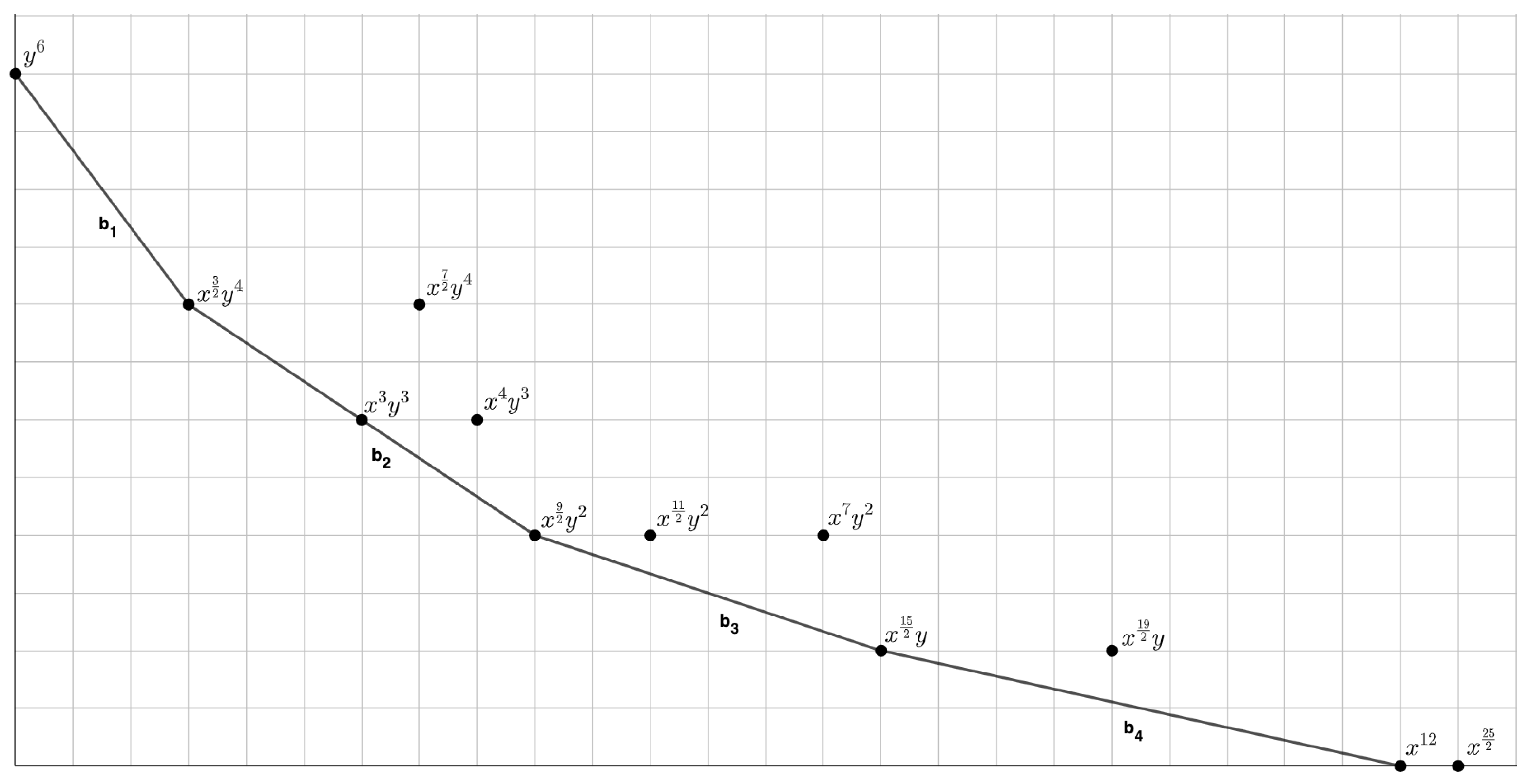
- Let be the leftmost point of (notice that is on the y-axis; if there are more points with abscissa 0, we choose the lowest one). From , we rotate a vertical downward ray counterclockwise and stop rotating it when it meets the first point of . We call the rightmost point of met by this ray;
- From , we rotate a vertical downward ray counterclockwise and we stop rotating it when it meets the first point of . We call the rightmost point of met by this ray;
- We repeat this procedure until we reach a point on the x-axis.

3. The Newton–Puiseux Algorithm
3.1. The ∗-Procedure and the Graph
- If , we ignore and we take into account uniquely the contribution given by the root of h, in the following way: we define a virtual Newton Polygon with just one edge and we set, with an abuse of notation:
- If , we take into account the contribution given by as well as the one given by the root , in the following way: being Newton-convenient, we can consider the Newton Polygon of and apply the procedure defined in Case to the Puiseux y-polynomial ; we rename the results of the procedure as follows:Moreover, we add a further virtual edge and we set, with an abuse of notation:
- (i)
- ;
- (ii)
- satysfies the assumptions of Theorem 1, i.e., the monomial z appears in with a non-zero coefficient (graphically, the Newton Polygon has a unique edge of height one).
3.2. The Paths on and the Branches of the Curve
- and are, respectively, the highest power of x and such that:
- is the chosen root of ;
- is the highest power of x such that
3.2.1. Each Path Gives the Approximation of a Branch
3.2.2. Justification of the Procedure
- (1)
- In the ∗-Procedure, we need , and the roots of need to be in , with of the form , ;
- (2)
- In order to keep applying the ∗-Procedure, we must show that the Puiseux z-polynomial satisfies .
- (1)
- , and the roots of need to be in , with of the form , ;
- (2)
- .
3.3. The Lemmata
3.4. The Algorithm
The Newton–Puiseux Algorithm
| Algorithm 1: Study of the branches at of a reduced plane curve of equation , , such that |
Input: : , . Output: Integers and such that possesses s branches at O, and each branch is approximated by . |
|
| Algorithm 2: Study of the branches at of a plane curve of equation , , (the irreducible decomposition of f), with , |
Input: : , . Output: Integers and , , such that possesses branches at O, and each branch is approximated by , . |
|
3.5. An Example
- We haveThus, we have two distinct roots of , namely, double and simple, and, as a consequence, two possible choice for :We havehence,The Newton polygon is given in Figure 4We have an unique edge , therefore, we obtainThere is an unique root of , which isThus, we haveThe Newton polygon is given in Figure 5.We have an unique edge and we obtain:whose roots areBy Lemma 3, choosing either or , the polynomial satisfies the hypothesis of Theorem 1; hence, by 3.1, we can stop. Sincewe obtainTherefore, we have the following parameterizationsWe have that , at O, so by Step 3 of the Algorithm with , we conclude that and are equivalent parameterizations of the same 2-branch of .
- *
We haveand hence,The Newton polygon is given in Figure 6.We can just choose obtainingwhose unique root isMoreover, satisfies the hypothesis of Theorem 1, therefore, by Remark 3.1, we can stop by obtaining the following root of fHence, we have the parameterizationwhich is a 1-branch of at O. - We haveHence, we have only one choice for , that is,Proceeding, we obtainThe Newton Polygon is given in Figure 7:We can only choose , obtainingwhose roots areBy Lemma 3, choosing either or , the polynomial satisfies the hypothesis of Theorem 1. Hence, by Remark 3.1, we can stop obtaining the following roots of fHence we have the parameterizationsthat give two distinct 1-branches of at O.
- We haveWe have just a choice for , that is,Proceeding, we obtainThe Newton polygon is given in Figure 8.We can only choose , obtainingwhose unique root isMoreover, satisfies the hypothesis of Theorem 1, therefore, by Remark 3.1, we can stop obtaining the following root of fwhich gives the parameterizationwhich is a 1-branch of at O.


4. Triple Points
4.1. Output of the Newton–Puiseux Algorithm for Triple Points
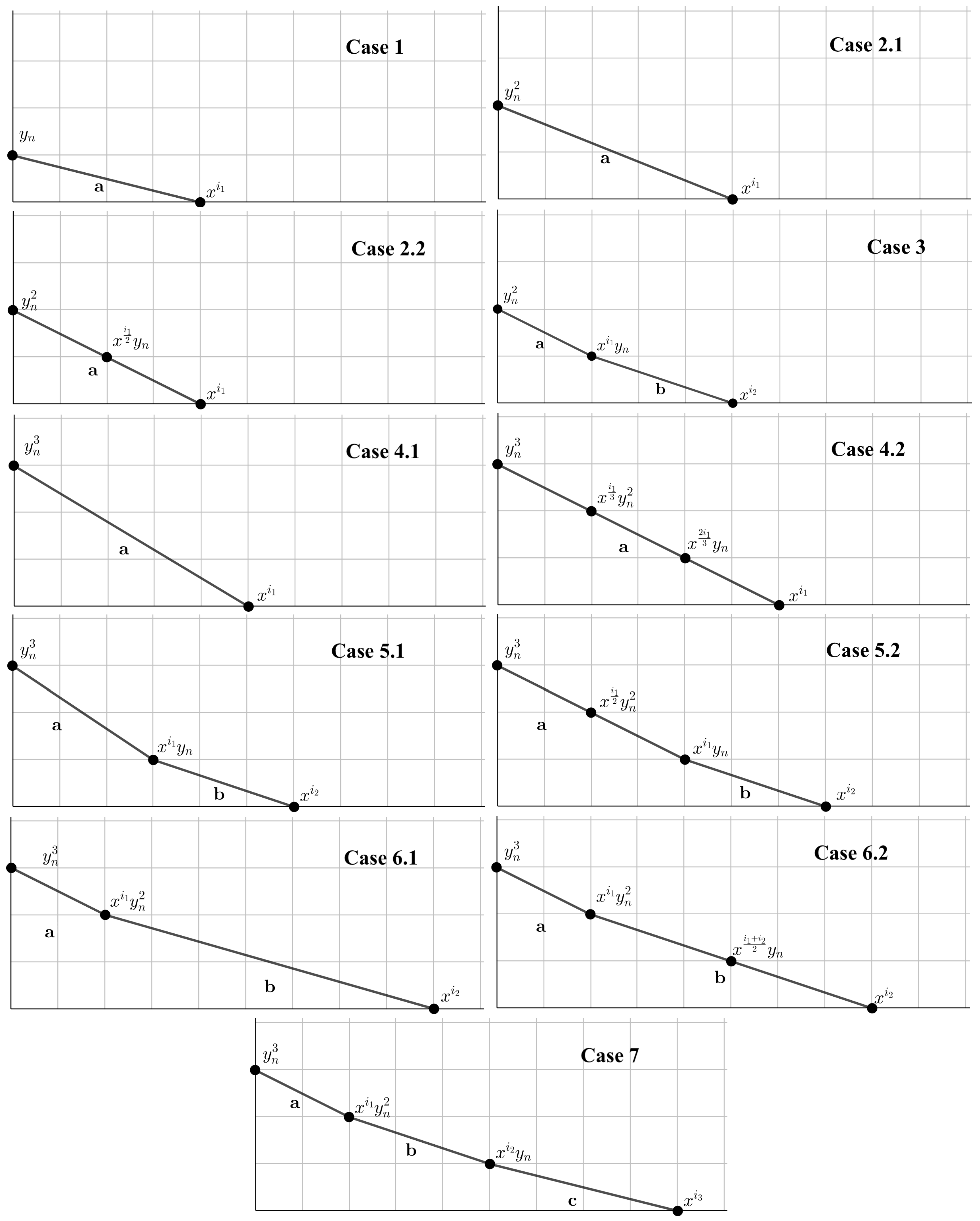
- 1.
- Which are the possible choices of and in each case?
- 2.
- When, for each choice of , does the algorithm stop?
- (i)
- Since the height of the Newton Polygon decreases at each step, i.e., , and , we have to consider Newton Polygons of height only;
- (ii)
- In general, . However, since , there exists such that . Hence, for , the vertices of are in .
4.2. A Theorem for Triple Points
Author Contributions
Funding
Informed Consent Statement
Data Availability Statement
Conflicts of Interest
References
- Bernardi, A.; Gimigliano, A.; Idà, M. Singularities of plane rational curves via projections. J. Symb. Comput. 2018, 86, 189–212. [Google Scholar] [CrossRef]
- Chen, F.; Wang, W.; Liu, Y. Computing singular points of plane rational curves. J. Symb. Comput. 2008, 43, 92–117. [Google Scholar] [CrossRef]
- Cox, D.; Kustin, A.R.; Polini, C.; Ulrich, B. A Study of singularities of rational curves via syzygies. Mem. Amer. Math. Soc. 2013, 222, 1045. [Google Scholar] [CrossRef]
- Puiseux, V.A. Recherches sur les fonctions algébriques. J. Math. Pures Appl. 1850, 15, 365–480. [Google Scholar]
- Newton, I. Letter from Newton to Oldenburg dated October 24, 1696. In The Correspondence of Isaak Newton; Cambridge University Press: Cambridge, UK, 1960; Volume 2, pp. 110–161. [Google Scholar]
- Newton, I. The Method of Fluxions and Infinite Series: With Its Application to the Geometry of Curve-Lines; John Nourse: London, UK, 1736. [Google Scholar]
- van der Waerden, B.L. Einfu¨hrung in Die Alebraische Geometrie; Springer: Berlin, Germany, 1939. [Google Scholar]
- Abhyankar, S.S. Algebraic Geometry for Scientists and Engineers; Mathematical Surveys and Monographs 35; A.M.S.: Providence, RI, USA, 1990. [Google Scholar]
- Walker, R.J. Algebraic Curves; Princeton University Press: Princeton, NJ, USA, 1950. [Google Scholar]
- Arrondo, E. Apuntes de Curvas Algebraicas. 2020. Available online: http://www.mat.ucm.es/~arrondo/curvas.pdf (accessed on 3 October 2022).
- Fischer, G. Plane Algebraic Curves; Kay, L., Translator; Student Math. Lib. AMS: Providence, RI, USA, 2001. [Google Scholar]
- Greuel, G.M.; Lossen, C.; Shustin, E. Introduction to Singularities and Deformations; Springer: Berlin/Heidelberg, Germany, 2007. [Google Scholar]
- Bassel, M.; Coquand, T. Dynamic Newton—Puiseux theorem. J. Log. Anal. 2013, 5, 1–22. [Google Scholar]
- Poteaux, A.; Rybowicz, M. Complexity bounds for the rational Newton-Puiseux algorithm over finite fields. AAECC 2011, 22, 187–217. [Google Scholar] [CrossRef]
- Poteaux, A.; Rybowicz, M. Good reduction of Puiseux series and applications. J. Symb. Comput. 2012, 47, 32–63. [Google Scholar] [CrossRef]
- Duval, D. Rational Puiseux expansions. Compos. Math. 1989, 70, 119–154. [Google Scholar]
- Manetti, M. Corso Introduttivo alla Geometria Algebrica; Scuola Normale Superiore di Pisa: Pisa, Italy, 1998; Available online: https://edizioni.sns.it/wp-content/uploads/2014/11/APPUNTI-MANETTI.pdf (accessed on 4 January 2023).
- Poteaux, A.; Weimann, M. Computing Puiseux series: A fast divide and conquer algorithm. Annales Henri Lebesgue 2021, 4, 1061–1102. [Google Scholar] [CrossRef]
- Oaku, T. Bernstein-Sato polynomials and analytic non-equivalence of plane curve singularities. arXiv 2022, arXiv:2207.00699. [Google Scholar]
- Hefez, A.; Hernandez, M.E. Classification of Plane Branches up to Multiplicity 4. J. Symb. Comput. 2009, 44, 626–634. [Google Scholar] [CrossRef]


Disclaimer/Publisher’s Note: The statements, opinions and data contained in all publications are solely those of the individual author(s) and contributor(s) and not of MDPI and/or the editor(s). MDPI and/or the editor(s) disclaim responsibility for any injury to people or property resulting from any ideas, methods, instructions or products referred to in the content. |
© 2023 by the authors. Licensee MDPI, Basel, Switzerland. This article is an open access article distributed under the terms and conditions of the Creative Commons Attribution (CC BY) license (https://creativecommons.org/licenses/by/4.0/).
Share and Cite
Canino, S.; Gimigliano, A.; Idà, M. The Newton–Puiseux Algorithm and Triple Points for Plane Curves. Mathematics 2023, 11, 2324. https://doi.org/10.3390/math11102324
Canino S, Gimigliano A, Idà M. The Newton–Puiseux Algorithm and Triple Points for Plane Curves. Mathematics. 2023; 11(10):2324. https://doi.org/10.3390/math11102324
Chicago/Turabian StyleCanino, Stefano, Alessandro Gimigliano, and Monica Idà. 2023. "The Newton–Puiseux Algorithm and Triple Points for Plane Curves" Mathematics 11, no. 10: 2324. https://doi.org/10.3390/math11102324