Statistical Inference on the Entropy Measures of Gamma Distribution under Progressive Censoring: EM and MCMC Algorithms

Abstract

Studying the ages of mobile phones is considered one of the most important things in the recent period in the field of shopping and modern technology. In this paper, we will consider that the ages of these phones follow a gamma distribution under progressive first-failure (PFF) censoring. All of the unknown parameters, as well as Shannon and Rényi entropies, were estimated for this distribution. The maximum likelihood (ML) approach was utilized to generate point estimates for the target parameters based on the considered censoring strategy. The asymptotic confidence intervals of the ML estimators (MLEs) of the targeted parameters were produced using the normal approximation to ML and log-transformed ML. We employed the delta method to approximate the variances of the Shannon and Rényi functions to obtain their asymptotic confidence intervals. Additionally, all parameter estimates utilized in this study were determined using the successful expectation–maximization (EM) method. The Metropolis–Hastings (MH) algorithm was applied to construct the Bayes estimators and related highest posterior density (HPD) credible intervals under various loss functions. Further, the proposed methodologies were contrasted using Monte Carlo simulations. Finally, the radio transceiver dataset was analyzed to substantiate our results.

1. Introduction

Smartphones have become an essential tool in our daily lives, but they do not last forever. The best phone goes through many problems before it dies, which makes you look for a new one. Therefore, when buying a new phone, it is necessary to know how long the phone will last before it dies. In this article, we will cover the lifespan of smartphones, considering that they follow a specific distribution, and we will estimate the parameters of this distribution and some important functions, such as the entropy function of this distribution, in order to provide some information that will benefit the companies designed for these devices, as well as to support decision makers in the field of technology to improve efficiency and to extend the life of these phones. In this study, we will consider that the lifetimes of phones follow the gamma distribution.

A continuous probability distribution called gamma is used to model continuous random variables (lifetimes of phones) with skewed distributions and fixed positive values. This group of continuous probability distributions has two parameters. The gamma distribution is exemplified in particular by the exponential, Erlang, and chi-squared distributions. It is extensively applied in a variety of application areas, such as engineering, the environment, meteorology, climatology, and other physical circumstances, as well as queuing theory and reliability theory (see Lawless [1]). The probability density function (PDF) of a gamma random variable (RV) is defined as follows:

$$f_X\left(x;\alpha ,\beta \right)=\frac{{\beta }^{\alpha }}{\Gamma \left(\alpha \right)}{x}^{\alpha -1}{e}^{-\beta x};x>0,\alpha >0,\beta >0,$$

(1)

where $\Gamma \left(\alpha \right)$ is the well-known gamma function defined by

$$\Gamma \left(\alpha \right)={\int }_0^{\infty }{x}^{\alpha -1}{e}^{-x}dx;\alpha >0,$$

and the corresponding cumulative distribution function (CDF) is given by

$$F_X\left(x;\alpha ,\beta \right)=1-\frac{\Gamma \left(\alpha ,\beta x\right)}{\Gamma \left(\alpha \right)};x>0,\alpha >0,\beta >0,$$

(2)

where $\Gamma \left(a,b\right)$ =${\int }_b^{\infty }{t}^{a-1}{e}^{-t}dt$ is the upper incomplete gamma function. The PDF of a gamma RV takes on a wide variety of shapes depending on the values of $\alpha$, also known as the shape parameter, and $\beta$ referred to as the inverse scale parameter, called a rate parameter. The hazard function shape of gamma distribution can be increased, decreased, or constant depending on $\alpha >1$, $\alpha <1$, or $\alpha =1$, respectively. When $\alpha =1$, the gamma RV becomes an exponential RV with parameter $\lambda$, and when $\alpha =\frac{n}{2}$, $n\in \mathbb{Z}$ and $\beta =\frac{1}{2}$, one can show that gamma RV decreases to the chi-square distribution with n degrees of freedom. Moreover, when $\alpha =n$ (integer), the gamma distribution is sometimes known as the Erlang distribution. In addition, the log-normal distribution is a limiting special case when $\alpha \to \infty$.

However, estimating the gamma parameters is still a complex issue. Recently, there have been many studies on the estimation procedure for the gamma distribution based on both complete and censored data. For instance, Son and Oh [2] proposed a Bayesian estimator using Gibbs sampling for the two-parameter gamma distribution based on a complete sample. Under the same sample, Pradhan and Kundu [3] studied the Bayes estimation and prediction of the two-parameter gamma distribution. Basak and Balakrishnan [4] considered some classical procedures to estimate the three-parameter gamma distribution using progressive Type-II samples. Bayesian inference for the capability index of the gamma distribution was developed by Almeida et al. [5]. Recently, Dey et al. [6] derived maximum likelihood and Bayes estimates of the unknown parameters of the gamma lifetime model based on progressive Type-II censoring, and also studied the problem of interval estimation.

Uncertainty about the time of death is part of the life of any product, and plays an important role in demographic and actuarial sciences. This paper analyzes death uncertainty through the concept of entropy. For more details on the concept of uncertainty and its applications, one can see Singh [7]. One way to define entropy in statistics is the expected value of the information content of a random variable. Information content, also known as subjective information or surprise, is a measure of the amount of information gained by observing the outcome of a random variable. The information content is inversely proportional to the probability of the outcome: the higher the probability of the outcome, the less information you provide; the outcome is less likely. There are several types of informational entropies. The concept of entropy was defined by Rényi [8]. For more details, see, Amigó et al. [9]. Here, we focus our attention on two of the most famous measures of entropy, namely the Shannon [10], and Rényi [8] entropies. If X is a continuous RV with PDF, say, $f\left(x\right)$, then the Shannon entropy “ShEn”, say, $H_{Sh}\left(f\right)$, is defined by

$$H_{Sh}\left(f\right)=-E\left[log{f}_X\left(x\right)\right]=-{\int }_X\left\{log{f}_X\left(x\right)\right\}{f}_X\left(x\right)dx$$

(3)

and the Rényi entropy “REn”, say, $H_R(\lambda ,f)$, is given by

$$H_R(\lambda ,f)=\frac{1}{1-\lambda }ln{\int }_X{f}_X{\left(x\right)}^{\lambda }dx,\lambda (\ne 1)>0.$$

(4)

Note that as $\lambda$ tends to one, $H_R(\lambda ,f)$ tends to $H_{Sh}\left(f\right)$. When $X\sim$gamma $(\alpha ,\beta )$, the $H_{Sh}\left(f\right)$ and $H_R(\lambda ,f)$ can be obtained as

$$H_{Sh}\left(f\right)=\alpha +log\Gamma \left(\alpha \right)-log\left(\beta \right)+(1-\alpha )\psi \left(\alpha \right)$$

(5)

and

$$H_R\left(\lambda \right)=-log\beta +\frac{1}{1-\lambda }log\left\{\frac{\Gamma \left(\lambda \alpha -\lambda +1\right)}{{\lambda }^{\lambda \alpha -\lambda +1}{\Gamma }^{\lambda }\left(\alpha \right)}\right\},\lambda \alpha -\lambda +1>0\mathrm{and}\lambda (\ne 1)>0,$$

(6)

where $\psi \left(\alpha \right)$ is the digamma function, given by

$$\psi \left(\alpha \right)=\frac{\partial log\Gamma \left(\alpha \right)}{\partial \alpha }=\underset{0}{\overset{\infty }{\int }}\left(log\alpha \right)x^{\alpha -1}{e}^{-x}dx=-\gamma -\frac{1}{\alpha }+\sum _{i=1}^{\infty }\left(\frac{1}{i}-\frac{1}{i+\alpha }\right),$$

and $\gamma \simeq 0.5772156649$ is known as Euler’s constant. As given by Acharya et al. [11], the Renyi entropy has many applications. Estimations of the Shannon and Renyi entropies have many applications in various fields; for example, in medicine, it is used in measuring genetic diversity, measuring neural activity, detecting cardiac autonomic neuropathy (CAN) in patients with diabetes (Cornforth et al. [12]), etc. Several authors have presented the problem of estimating entropy functions for different distributions under various samples. Among them, Kang et al. [13] introduced estimators of entropy for a double exponential distribution when the samples are multiplying Type-II censored samples. Cho et al. [14] estimated the ShEn function of the Rayleigh distribution based on doubly generalized Type II hybrid censored samples. Based on generalized Type II hybrid censored samples, Cho et al. [15] derived estimators for the entropy function of a Weibull distribution. The estimated entropy for a generalized exponential distribution under record values is obtained by Chacko [16]. Liu and Gui [17] investigated the ShEn for Lomax distribution based on a generalized progressive hybrid censoring scheme. Furthermore, statistical inference on the ShEn of the inverse Weibull distribution under PFF censoring was considered by Yu et al. [18]. One of the main objectives of this research is to estimate the ShEn and REn of gamma distribution based on progressive first-failure censoring data.

Life-testing experiments are powerful tools in modern science and technology for gaining comprehensive knowledge of products. It is challenging to obtain comprehensive information about every failed unit in the life-testing experiment. The sampling process is condensed by the particular censoring method set in advance to save time and cut costs. The final sample we obtain is known as a censored sample. Censoring is a highly prevalent occurrence that has been exploited extensively in the fields of industrial engineering, biology, clinical trials, radio interference, etc. It has been shown through various life experiences that both statistical inference and cost savings can be achieved by designing a reasonably effective censoring system. The most popular censoring techniques among the numerous approaches are Type-I and Type-II with its PFF schemes. For more information see, Balakrishnan and Aggarwala [19], Wu and Kus [20], Dube et al. [21], Maurya et al. [22], and references cited therein. In the PFF censoring scheme, we randomly divide N($N=n\times k$) units into n groups, with each group containing k independent units. We observe these n groups simultaneously and independently. Now, let the failure times of $n\times k$ items under the study have a continuous PDF $f_X\left(x\right|\theta )$ and CDF $F_X\left(x\right|\theta )$; the joint PDF of $X_{1:m:n:k}<X_{2:m:n:k}<\cdots <X_{m:m:n:k}$ can be formulated as

$$L_{X_{1;m:n:k},\dots ,X_{m;m:n:k}}\left(\theta |x_{1:m:n:k},\dots ,x_{m:m:n:k}\right)=A{k}^m\prod _{i=1}^{m}f\left(x_{i;m:n:k}|\theta \right){\left[1-F\left(x_{i;m:n:k}|\theta \right)\right]}^{k\left(R_i+1\right)-1},$$

(7)

where $A=n(n-R_1-1)(n-R_1-R_2-1)\dots (n-R_1-R_2-\dots -m+1)$.

In this study, we consider PFF censoring because of its good generalization behavior with other censoring plans. To the best of our knowledge, there are not any papers dealing with the estimation of the gamma distribution parameters based on PFF censoring.

2. Maximum Likelihood Estimators

This approach can be used to search the space of possible distributions and parameters. The goal of maximum-likelihood (ML) estimation is to find those parameter values of the model that maximize the probability function over the parameter space. The specific value that maximizes the probability function is called the maximum likelihood estimate. The maximum likelihood method is a mainstream method of statistical inference and can be applied to different types of distributions and models. Due to their asymptotic properties, confidence intervals (CIs) can be derived based on Fisher information matrix (FIM).

2.1. Likelihood Equations

Let $X_{1;m:n:k},X_{2;m:n:k},\dots ,X_{m;m:n:k}$ be PFF censored samples from gamma($\alpha ,\beta$) distribution with censoring scheme $\Re =(R_1,R_2,\dots ,R_m)$, effective sample size m, number of groups n, and group size k. We use $x_i$ instead of $X_{i;m:n:k}$ to simplify notation. The observed data are $\underline{x}=(x_{1;m:n:k},x_{2;m:n:k},\dots ,x_{m;m:n:k})$, and from (7), the likelihood function, say, $L\left(\alpha ,\beta |\underline{x}\right)$, can be listed as

$$L\left(\alpha ,\beta |\underline{x}\right)=A{k}^m\prod _{i=1}^m\frac{{\beta }^{\alpha }}{\Gamma \left(\alpha \right)}{x}^{\alpha -1}{e}^{-\beta x}{\left[\frac{\Gamma \left(\alpha ,\beta x\right)}{\Gamma \left(\alpha \right)}\right]}^{k\left(R_i+1\right)-1}.$$

(8)

The log-likelihood function, say, $\ell \left(\alpha ,\beta |\underline{x}\right)$, can be written as

$$\ell \left(\alpha ,\beta |\underline{x}\right)\propto m\alpha log\beta +\left(\alpha -1\right)\sum _{i=1}^{m}log{x}_i-\beta \sum _{i=1}^m{x}_i-Nlog\Gamma \left(\alpha \right)+\sum _{i=1}^m\left(k\left(R_i+1\right)-1\right)log\Gamma \left(\alpha ,\beta x_i\right),$$

(9)

where $N=nk$. The partial derivatives of $\ell \left(\alpha ,\beta |\underline{x}\right)$ with respect to $\alpha$ and $\beta$ are set equal to zero to determine the MLEs of $\alpha$ and $\beta$. Thus, we have the following:

$$\frac{\partial \ell \left(\alpha ,\beta |\underline{x}\right)}{\partial \alpha }=mlog\beta +\sum _{i=1}^{m}log{x}_i-N\psi \left(\alpha \right)+\sum _{i=1}^m\left(k\left(R_i+1\right)-1\right){\phi }_{1i}\left(\alpha ,\beta \right)=0$$

(10)

and

$$\frac{\partial \ell \left(\alpha ,\beta |\underline{x}\right)}{\partial \beta }=\frac{m\alpha }{\beta }-\sum _{i=1}^m{x}_i-\sum _{i=1}^m\left(k\left(R_i+1\right)-1\right){\phi }_{2i}\left(\alpha ,\beta \right)=0,$$

(11)

where

$${\phi }_{1i}\left(\alpha ,\beta \right)=log\left(\beta x_i\right)+\frac{1}{\Gamma \left(\alpha ,\beta x_i\right)}{G}_{2,3}^{3,0}\left(\beta t\left|\begin{array}{c}1,1\\ 0,0,\alpha \end{array}\right.\right)$$

(12)

and

$${\phi }_{2i}\left(\alpha ,\beta \right)=\frac{\partial log\Gamma \left(\alpha ,\beta x_i\right)}{\partial \beta }=\frac{{\beta }^{\alpha +1}{x}_i^{\alpha }{e}^{-\beta x_i}}{\Gamma \left(\alpha ,\beta x_i\right)},$$

(13)

where $\psi \left(\alpha \right)=\frac{\partial \Gamma \left(\alpha \right)}{\partial \alpha }\sim log\left(\alpha \right)-\frac{1}{2\alpha }$ is the digamma function and $G_{2,3}^{3,0}\left(.\right)$ is Meijer’s G-function. For the definition and properties of Meijer’s G-function, we refer to Mathai [23] and Askey [24]. Clearly, the roots of the nonlinear (10) and (11) cannot yield solutions to $\alpha$ and $\beta$ in a closed form, so some numerical techniques, such as the Newton–Raphson (NR) method, are employed to derive the MLEs (${\widehat{\alpha }}_{ML}$ and ${\widehat{\beta }}_{ML}$). The MLEs of the $H_{Sh}\left(f\right)$ and $H_R\left(\lambda \right)$ are obtained using the invariance property of MLEs, such as

$${\widehat{H}}_{Sh}\left(f\right)={\widehat{\alpha }}_{ML}+log\Gamma \left({\widehat{\alpha }}_{ML}\right)-log{\widehat{\beta }}_{ML}+(1-{\widehat{\alpha }}_{ML})\psi \left({\widehat{\alpha }}_{ML}\right)$$

(14)

and

$${\widehat{H}}_R\left(\lambda \right)=-log{\widehat{\beta }}_{ML}+\frac{1}{1-\lambda }log\left\{\frac{\Gamma \left[\lambda {\widehat{\alpha }}_{ML}-\lambda +1\right]}{{\lambda }^{\lambda {\widehat{\alpha }}_{ML}-\lambda +1}{\Gamma }^{\lambda }\left({\widehat{\alpha }}_{ML}\right)}\right\}.$$

(15)

2.2. Asymptotic Confidence Intervals for MLEs

As discussed in the previous section, the MLE specifies a single value of the unknown parameter. The single value (point estimate) gives no indication as to the accuracy of the estimate, and falls short of providing the confidence placed on it. So, we have to use the interval estimate. The ACIs of $\alpha$ and $\beta$ can be established by using the asymptotic variances of MLEs, say, $\widehat{V}ar\left({\widehat{\alpha }}_{ML}\right)$ and $\widehat{V}ar\left({\widehat{\beta }}_{ML}\right)$, which can be obtained from the inverse FIM. Let $\theta =(\alpha ,\beta )$, then the FIM, say, $I\left(\theta \right)$, can be written as

$$I\left(\theta \right)=E\left[\begin{array}{cc}-\frac{{\partial }^2\ell \left(\alpha ,\beta |\underline{x}\right)}{{\partial }^2{\alpha }^2}& -\frac{{\partial }^2\ell \left(\alpha ,\beta |\underline{x}\right)}{\partial \alpha \partial \beta }\\ -\frac{{\partial }^2\ell \left(\alpha ,\beta |\underline{x}\right)}{\partial \alpha \partial \beta }& -\frac{{\partial }^2\ell \left(\alpha ,\beta |\underline{x}\right)}{{\partial }^2{\beta }^2}\end{array}\right].$$

(16)

where

$$\frac{{\partial }^2\ell \left(\alpha ,\beta |\underline{x}\right)}{{\partial }^2{\alpha }^2}=-N{\psi }^{\left(1\right)}\left(\alpha \right)+\sum _{i=1}^m\left(k\left(R_i+1\right)-1\right){\Omega }_{1i}\left(\alpha ,\beta \right),$$

$$\frac{{\partial }^2\ell \left(\alpha ,\beta |\underline{x}\right)}{\partial \alpha \partial \beta }=\frac{m}{\beta }-\sum _{i=1}^m\left(k\left(R_i+1\right)-1\right){\Omega }_{2i}\left(\alpha ,\beta \right)$$

and

$$\frac{{\partial }^2\ell \left(\alpha ,\beta |\underline{x}\right)}{{\partial }^2{\beta }^2}=\frac{-m\alpha }{{\beta }^2}+\sum _{i=1}^m\left(k\left(R_i+1\right)-1\right){\Omega }_3\left(\alpha ,\beta x_i\right).$$

where ${\psi }^{\left(1\right)}\left(\alpha \right)=\frac{{\partial }^2\Gamma \left(\alpha \right)}{\partial {\alpha }^2}$ is the tri-gamma function. It may also be defined as the sum of the series ${\sum }_{i=1}^{\infty }{\left(\alpha +i\right)}^{-2},$

$$\begin{array}{ccc}\hfill {\Omega }_{1i}\left(\alpha ,\beta \right)& =& \frac{{\partial }^2\Gamma \left(\alpha ,\beta x_i\right)}{{\partial }^2{\alpha }^2}\hfill \\ & =& \frac{2G_{3,4}^{4,0}\left(\beta x_i\left|\begin{array}{c}1,1,1\\ 0,0,0,\alpha \end{array}\right.\right)+2log\left(\beta x_i\right)G_{2,3}^{3,0}\left(\beta x_j\left|\begin{array}{c}1,1\\ 0,0,\alpha \end{array}\right.\right)}{\Gamma \left(\alpha ,\beta x_i\right)}+log{\left(\beta x_i\right)}^2-{\left[{\phi }_{1i}\left(\alpha ,\beta \right)\right]}^2,\hfill \end{array}$$

$${\Omega }_{2i}\left(\alpha ,\beta \right)=\frac{{\partial }^2\Gamma \left(\alpha ,\beta x_i\right)}{\partial \alpha \partial \beta }={\phi }_{2i}\left(\alpha ,\beta \right)\left\{{\phi }_{1i}\left(\alpha ,\beta \right)-log\left(\beta x_i\right)\right\}$$

and

$${\Omega }_3\left(\alpha ,\beta x_i\right)=\frac{{\partial }^2\Gamma \left(\alpha ,\beta x_i\right)}{\partial {\beta }^2}={\phi }_{2i}\left(\alpha ,\beta \right)\left\{x_i-\alpha -1-{\phi }_{2i}\left(\alpha ,\beta \right)\right\},$$

where ${\phi }_{1i}\left(\alpha ,\beta \right)$ and ${\phi }_{2i}\left(\alpha ,\beta \right)$ are given, respectively, by (12) and (13). Let $\widehat{\theta }=({\widehat{\alpha }}_{ML},{\widehat{\beta }}_{ML})$ be the MLEs of the parameters $\theta =(\alpha ,\beta )$. Then, the observed FIM can be listed as

$$I\left(\widehat{\theta }\right)={\left[\begin{array}{cc}-\frac{{\partial }^2\ell \left(\alpha ,\beta |\underline{x}\right)}{{\partial }^2{\alpha }^2}& -\frac{{\partial }^2\ell \left(\alpha ,\beta |\underline{x}\right)}{\partial \alpha \partial \beta }\\ -\frac{{\partial }^2\ell \left(\alpha ,\beta |\underline{x}\right)}{\partial \alpha \partial \beta }& -\frac{{\partial }^2\ell \left(\alpha ,\beta |\underline{x}\right)}{{\partial }^2{\beta }^2}\end{array}\right]}_{(\alpha ,\beta )=({\widehat{\alpha }}_{ML},{\widehat{\beta }}_{ML})}.$$

Thus,

$$I^{-1}\left(\widehat{\theta }\right)=\left[\begin{array}{cc}\widehat{V}ar\left({\widehat{\alpha }}_{ML}\right)& \widehat{C}ov\left({\widehat{\alpha }}_{ML},{\widehat{\beta }}_{ML}\right)\\ \widehat{C}ov\left({\widehat{\alpha }}_{ML},{\widehat{\beta }}_{ML}\right)& \widehat{V}ar\left({\widehat{\beta }}_{ML}\right)\end{array}\right].$$

(17)

Therefore, the two-sided equal tail asymptotic $100(1-\tau )\%$ CIs of $\alpha$ and $\beta$ are, respectively, given by

$${\widehat{\alpha }}_{ML}\pm Z_{\frac{\tau }{2}}\sqrt{\widehat{V}ar\left({\widehat{\alpha }}_{ML}\right)}\mathrm{and}{\widehat{\beta }}_{ML}\pm Z_{\frac{\tau }{2}}\sqrt{\widehat{V}ar\left({\widehat{\beta }}_{ML}\right)},$$

(18)

To get the approximate estimation of the variance of ShEn and REn, the delta approach can be applied. Let

$$D_{H_{Sh}}={\left(\frac{\partial H_{Sh}\left(f\right)}{\partial \alpha },\frac{\partial H_{Sh}\left(f\right)}{\partial \beta }\right)}_{\alpha ={\widehat{\alpha }}_{ML},\beta ={\widehat{\beta }}_{ML}}\mathrm{and}{D}_{H_R}={\left(\frac{\partial H_R\left(\lambda \right)}{\partial \alpha },\frac{\partial H_R\left(\lambda \right)}{\partial \beta }\right)}_{\alpha ={\widehat{\alpha }}_{ML},\beta ={\widehat{\beta }}_{ML}}.$$

Calculate the estimated variance of ${\widehat{H}}_{Sh}\left(f\right)$ and ${\widehat{H}}_R\left(\lambda \right)$ as

$$\widehat{V}ar\left({\widehat{H}}_{Sh}\left(f\right)\right)=D_{H_{Sh}}{I}^{-1}({\widehat{\alpha }}_{ML},{\widehat{\beta }}_{ML})D_{H_{Sh}}^T\mathrm{and}\widehat{V}ar\left({\widehat{H}}_R\left(\lambda \right)\right)=D_{H_R}{I}^{-1}({\widehat{\alpha }}_{ML},{\widehat{\beta }}_{ML})D_{H_R}^T,$$

where $D^T$ is the transpose of matrix D. Then, we obtain the $100(1-\tau )\%$ two-sided asymptotic approximate CIs for ShEn and REn, respectively, in the following forms:

$$\left({\widehat{H}}_{Sh}\left(f\right)-Z_{\frac{\tau }{2}}\sqrt{\widehat{V}ar({\widehat{H}}_{Sh}\left(f\right)},{\widehat{H}}_{Sh}\left(f\right)+Z_{\frac{\tau }{2}}\sqrt{\widehat{V}ar\left({\widehat{H}}_{Sh}\left(f\right)\right)}\right)$$

(19)

and

$$\left({\widehat{H}}_R\left(\lambda \right)-Z_{\frac{\tau }{2}}\sqrt{\widehat{V}ar\left({\widehat{H}}_R\left(\lambda \right)\right)},{\widehat{H}}_R\left(\lambda \right)+Z_{\frac{\tau }{2}}\sqrt{\widehat{V}ar\left({\widehat{H}}_R\left(\lambda \right)\right)}\right).$$

(20)

It is well known in the literature that the approximate CIs dependent on the logarithmically transformed MLE method have the potential to provide more accurate coverage (see Meeker and Escobar [25]); consequently, in the following subsection, we will derive the approximate CIs of $\alpha ,$$\beta ,$$H_{Sh}\left(f\right)$ and $H_R\left(\lambda \right)$ based on this method, and we rely on them to provide simulation studies and numerical examples.

2.3. Asymptotic Confidence Intervals for Log-Transformed MLEs

The two-sided $100(1-\tau )\%$ log-normal approximation confidence intervals for positive parameters $\alpha$ and $\beta$ are given by

$$\left[{\widehat{\alpha }}_{ML}exp\left(-\frac{Z_{(1-\gamma /2)}\sqrt{\widehat{V}ar\left({\widehat{\alpha }}_{ML}\right)}}{{\widehat{\alpha }}_{ML}}\right),{\widehat{\alpha }}_{ML}exp\left(\frac{Z_{(1-\gamma /2)}\sqrt{\widehat{V}ar\left({\widehat{\alpha }}_{ML}\right)}}{{\widehat{\alpha }}_{ML}}\right)\right]$$

(21)

and

$$\left[{\widehat{\beta }}_{ML}exp\left(-\frac{Z_{(1-\gamma /2)}\sqrt{\widehat{V}ar\left({\widehat{\beta }}_{ML}\right)}}{{\widehat{\beta }}_{ML}}\right),{\widehat{\beta }}_{ML}exp\left(\frac{Z_{(1-\gamma /2)}\sqrt{\widehat{V}ar\left({\widehat{\beta }}_{ML}\right)}}{{\widehat{\beta }}_{ML}}\right)\right].$$

(22)

Following the same procedure, the two-sided $100(1-\tau )\%$ log-normal approximation CIs for ShEn and REn can be constructed as

$$\left[{\widehat{H}}_{Sh}\left(f\right)exp\left(-\frac{Z_{(1-\tau /2)}\sqrt{\widehat{V}ar\left({\widehat{H}}_{Sh}\left(f\right)\right)}}{{\widehat{H}}_{Sh}\left(f\right)}\right),{\widehat{H}}_{Sh}\left(f\right)exp\left(\frac{Z_{(1-\tau /2)}\sqrt{\widehat{V}ar\left({\widehat{H}}_{Sh}\left(f\right)\right)}}{{\widehat{H}}_{Sh}\left(f\right)}\right)\right]$$

(23)

and

$$\left[{\widehat{H}}_R\left(\lambda \right)exp\left(-\frac{Z_{(1-\tau /2)}\sqrt{\widehat{V}ar\left({\widehat{H}}_R\left(\lambda \right)\right)}}{{\widehat{H}}_R\left(\lambda \right)}\right),{\widehat{H}}_R\left(\lambda \right)exp\left(\frac{Z_{(1-\tau /2)}\sqrt{\widehat{V}ar\left({\widehat{H}}_R\left(\lambda \right)\right)}}{{\widehat{H}}_R\left(\lambda \right)}\right)\right],$$

(24)

where $\widehat{V}ar\left({\widehat{H}}_{Sh}\left(f\right)\right)$ is the estimated variance of $H_{Sh}\left(f\right)$ and $\widehat{V}ar\left({\widehat{H}}_R\left(\lambda \right)\right)$ is the estimated variance of $H_R\left(\lambda \right)$, which can be calculated by the delta method. In the next section, we will develop an EM algorithm for computing the MLEs of the $\alpha ,$$\beta$, $H_{Sh}\left(f\right)$ and $H_R\left(\lambda \right)$ and their CIs.

3. Expectation–Maximization Algorithm

The EM algorithm was presented mathematically in detail by Dempster et al. [26] whereas for its application to PFF see, Ng et al. [27]. Suppose that $W=(X,Y)$ consists of observable $X=(X_{1;m:n:k},\dots ,X_{m;m:n:k})$ data and censored observations ($Y_1,\dots ,Y_m$) data, with $Y_j$ being a $1\times \left(k(R_j+1)-1\right)$ vector, such that $Y_j=$($Y_{j_1},Y_{j_2},\dots ,Y_{j_{\left(k(R_j+1)-1\right)}}$), $j=1,\dots ,m$. The likelihood function, say, $L_{\mathbf{C}}\left(W;\alpha ,\beta \right)$, of the complete data is given by

$$\begin{array}{ccc}{L}_{\mathbf{C}}\left(W;\alpha ,\beta \right)& \propto & {\displaystyle \prod _{i=1}^m}f\left(x_{i;m:n:k}|\alpha ,\beta \right){\displaystyle \prod _{i=1}^m}{\displaystyle \prod _{j=1}^{k\left[R_i+1\right]-1}}f\left(y_{ij}|\alpha ,\beta \right)\hfill \\ & \propto & \frac{{\beta }^{N\alpha }}{{\Gamma }^N\left(\alpha \right)}{\displaystyle \prod _{i=1}^m}{x}_i^{\alpha -1}{\displaystyle \prod _{i=1}^m}{\displaystyle \prod _{j=1}^{k\left[R_i+1\right]-1}}{y}_{ij}^{\alpha -1}exp\left[-\beta \left({\sum }_{i=1}^m{x}_i+{\sum }_{i=1}^m{\sum }_{i=1}^{k\left[R_i+1\right]-1}{y}_{ij}\right)\right].\hfill \end{array}$$

The log-likelihood for the complete lifetimes of $N=nk$ items from the two parameters gamma distribution, say, ${\ell }_c\left(W;\alpha ,\beta \right)$, can be represented as

$$\begin{array}{ccc}{\ell }_c\left(W;\alpha ,\beta \right)& \propto & N\alpha log\beta -Nlog\Gamma \left(\alpha \right)+\left(\alpha -1\right)\left[{\displaystyle \sum _{i=1}^m}log{x}_i+{\displaystyle \sum _{i=1}^m}{\displaystyle \sum _{i=1}^{k\left[R_i+1\right]-1}}log{y}_{ij}\right]\hfill \\ & & -\beta \left[{\displaystyle \sum _{i=1}^m}{x}_i+{\displaystyle \sum _{i=1}^m}{\displaystyle \sum _{i=1}^{k\left[R_i+1\right]-1}}{y}_{ij}\right].\hfill \end{array}$$

(25)

The E-step involves the computation of the conditional expectation $E\left({\ell }_c\left(W;\alpha ,\beta \right)\right|X)$, which is equal to the pseudo ${\ell }_s\left(W;\alpha ,\beta \right)$, defined as

$$\begin{array}{ccc}{\ell }_s\left(W;\alpha ,\beta \right)& \propto & N\alpha log\beta -Nlog\Gamma \left(\alpha \right)+\left(\alpha -1\right)\left[{\displaystyle \sum _{i=1}^m}log{x}_i+{\displaystyle \sum _{i=1}^m}{\displaystyle \sum _{i=1}^{k\left[R_i+1\right]-1}}E\left[log{y}_{ij}|y_{ij}>x_i\right]\right]\hfill \\ & & -\beta \left[{\displaystyle \sum _{i=1}^m}{x}_i+{\displaystyle \sum _{i=1}^m}{\displaystyle \sum _{i=1}^{k\left[R_i+1\right]-1}}E\left[y_{ij}|y_{ij}>x_i\right]\right].\hfill \end{array}$$

(26)

Then, the E-step needs the computation of $E\left(log{y}_{ij}|x_i\right)$ and $E\left(y_{ij}|x_i\right)$, where, the conditional probability function of the censored data, given the observed data, can be obtained [24] as follows:

$$f_{Y|X}\left(y_{ij}\right|x_i,\alpha ,\beta )=\frac{f(y_{ij},\alpha ,\beta )}{1-F(x_i,\alpha ,\beta )},y_{ij}>x_i,i=1,2,\dots ,m.$$

(27)

Given that $t=x_i$ for $i=1,2,\dots ,m$, the required expected values of a truncated gamma from the left at t are, respectively, given by

$$\begin{array}{ccc}E\left(log{y}_{ij}|x_i\right)& =& {\epsilon }_1\left(t,\alpha ,\beta \right)=\frac{1}{1-F(t,\alpha ,\beta )}{\int }_t^{\infty }\left(logz\right)f(z,\alpha ,\beta )dz\hfill \\ & =& \frac{1}{1-F(t,\alpha ,\beta )}{\int }_t^{\infty }\left(logz\right)\frac{{\beta }^{\alpha }}{\Gamma \left(\alpha \right)}{z}^{\alpha -1}{e}^{-\beta z}dz\hfill \\ & =& log\left(t\right)+\frac{1}{\Gamma \left(\alpha ,\beta t\right)}{G}_{2,3}^{3,0}\left(\beta t\left|\begin{array}{c}1,1\\ 0,0,\alpha \end{array}\right.\right)\hfill \end{array}$$

(28)

and

$$E\left(y_{ij}|x_i\right)={\epsilon }_2\left(t,\alpha ,\beta \right)=\frac{1}{1-F(t,\alpha ,\beta )}{\int }_t^{\infty }zf(z,\alpha ,\beta )dz=\frac{\Gamma \left[\alpha +1,\beta t\right]}{\beta \Gamma \left(\alpha ,\beta t\right)}.$$

(29)

The M-step deals with maximization of ${\ell }_s\left(W;\alpha ,\beta \right)$ with respect to $\alpha$ and $\beta$. Let the $rth$-stage estimate of ($\alpha ,\beta$) be (${\alpha }_{\left(r\right)},{\beta }_{\left(r\right)}$); then, next updated estimate (${\alpha }_{(r+1)},{\beta }_{(r+1)}$) is obtained by maximizing the following equation:

$$\begin{array}{ccc}Q\left({\alpha }_{\left(r\right)},{\beta }_{\left(r\right)}\right)& \propto & N\alpha log\beta -Nlog\Gamma \left(\alpha \right)+\left(\alpha -1\right){\displaystyle \sum _{i=1}^m}(k\left[R_i+1\right]-1){\epsilon }_1\left(x_i,{\alpha }_{\left(r\right)},{\beta }_{\left(r\right)}\right)\hfill \\ & & +\left(\alpha -1\right){\displaystyle \sum _{i=1}^m}log{x}_i-\beta {\displaystyle \sum _{i=1}^m}{x}_i-\beta {\displaystyle \sum _{i=1}^m}(k\left[R_i+1\right]-1){\epsilon }_2\left(x_i,{\alpha }_{\left(r\right)},{\beta }_{\left(r\right)}\right).\hfill \end{array}$$

(30)

By taking the derivatives of (30) with respect to $\alpha$ and $\beta$, respectively, and equating them to zero, as follows:

$$\frac{\partial Q\left(\alpha ,\beta \right)}{\partial \alpha }=Nlog\beta -N\psi \left(\alpha \right)+\sum _{i=1}^{m}log{x}_i+\sum _{i=1}^m(k\left[R_i+1\right]-1){\epsilon }_1\left(x_i,{\alpha }_{\left(r\right)},{\beta }_{\left(r\right)}\right)=0$$

(31)

and

$$\frac{\partial Q\left(\alpha ,\beta \right)}{\partial \beta }=\frac{N\alpha }{\beta }-\sum _{i=1}^m{x}_i-\sum _{i=1}^m(k\left[R_i+1\right]-1){\epsilon }_2\left(x_i,{\alpha }_{\left(r\right)},{\beta }_{\left(r\right)}\right)=0.$$

(32)

From (31),

$$log\beta -\psi \left(\alpha \right)=\frac{-1}{N}\left[\sum _{i=1}^{m}log{x}_i+\sum _{i=1}^m(k\left[R_i+1\right]-1){\epsilon }_1\left(x_i,{\alpha }_{\left(r\right)},{\beta }_{\left(r\right)}\right)\right]$$

(33)

and from (33),

$$\frac{\alpha }{\beta }=\frac{1}{N}\left[\sum _{i=1}^m{x}_i+\sum _{i=1}^m(k\left[R_i+1\right]-1){\epsilon }_2\left(x_i,{\alpha }_{\left(r\right)},{\beta }_{\left(r\right)}\right)\right],$$

or equivalently,

$$log\beta =log\alpha -log\left\{\frac{1}{N}\left[\sum _{i=1}^m{x}_i+\sum _{i=1}^m(k\left[R_i+1\right]-1){\epsilon }_2\left(x_i,{\alpha }_{\left(r\right)},{\beta }_{\left(r\right)}\right)\right]\right\}.$$

(34)

Substituting from (34) in (33), we have

$$\begin{array}{ccc}\hfill log\alpha -\psi \left(\alpha \right)& =& log\left\{\frac{1}{N}\left[\sum _{i=1}^m{x}_i+\sum _{i=1}^m(k\left[R_i+1\right]-1){\epsilon }_2\left(x_i,{\alpha }_{\left(r\right)},{\beta }_{\left(r\right)}\right)\right]\right\}\hfill \\ & & -\frac{1}{N}\left[\sum _{i=1}^{m}log{x}_i+\sum _{i=1}^m(k\left[R_i+1\right]-1){\epsilon }_1\left(x_i,{\alpha }_{\left(r\right)},{\beta }_{\left(r\right)}\right)\right].\hfill \end{array}$$

We observe that the updated estimate ${\alpha }_{(r+1)}$ of $\alpha$ can be computed from the fixed-point method, for which we solve the equation

$$g\left(\alpha \right)=\alpha ,$$

(35)

where

$$\begin{array}{ccc}\hfill g\left(\alpha \right)& =& exp\left\{\psi \left(\alpha \right)+log\left\{\frac{1}{N}\left[\sum _{i=1}^m{x}_i+\sum _{i=1}^m(k\left[R_i+1\right]-1){\epsilon }_2\left(x_i,{\alpha }_{\left(r\right)},{\beta }_{\left(r\right)}\right)\right]\right\}\right.\hfill \\ & & \left.-\frac{1}{N}\left[\sum _{i=1}^{m}log{x}_i+\sum _{i=1}^m(k\left[R_i+1\right]-1){\epsilon }_1\left(x_i,{\alpha }_{\left(r\right)},{\beta }_{\left(r\right)}\right)\right]\right\}\hfill \end{array}$$

and

$$\widehat{\beta }\left(\alpha \right)=N\alpha {\left[\sum _{i=1}^m{x}_i+\sum _{i=1}^m(k\left[R_i+1\right]-1){\epsilon }_2\left(x_i,{\alpha }_{\left(r\right)},{\beta }_{\left(r\right)}\right)\right]}^{-1}.$$

(36)

It is observed that ${\beta }_{(r+1)}$ can be obtained from (36). Then, (${\alpha }_{(r+1)}$, ${\beta }_{(r+1)}$) are used as the current estimates of ($\alpha ,\beta$) in the next iteration. The MLEs of ($\alpha ,\beta$) can be obtained by repeating the E-step and M-step until convergence is achieved. We stop the iterations when $Max[\left|{\alpha }_{(r+1)}-{\alpha }_{\left(r\right)}\right|+\left|{\beta }_{(r+1)}-{\beta }_{\left(r\right)}\right|]<\in$, where ∈ is the tolerance limit.

According to the Corollary in McLachlan et al. [28] (page 84), the proposed EM estimator sequence converges to the unique maximizer of the log-likelihood function. Using the obtained point estimators of $\alpha$, $\beta$ and the invariance property of MLEs, we can derive the estimates for the ShEn and REn measures, which are given as follows:

$${\widehat{H}}_{S{h}_{EM}}\left(f\right)={\alpha }_{(r+1)}+log\Gamma \left({\alpha }_{(r+1)}\right)-log\left({\beta }_{(r+1)}\right)+(1-{\alpha }_{(r+1)})\psi \left({\alpha }_{(r+1)}\right)$$

(37)

and

$${\widehat{H}}_{R_{RM}}\left(\lambda \right)=-ln{\beta }_{(r+1)}+\frac{1}{1-\lambda }ln\frac{\Gamma \left[\lambda {\alpha }_{(r+1)}-\lambda +1\right]}{{\lambda }^{\lambda {\alpha }_{(r+1)}-\lambda +1}{\Gamma }^{\lambda }\left({\alpha }_{(r+1)}\right)}.$$

(38)

Fisher Information Matrix via EM Algorithm

FIM plays an important role in the statistical inference of unknown parameters.let us denote the observed, missing, and complete information by $I_X\left(\theta \right)$, $I_{W|X}\left(\theta \right)$, and $I_W\left(\theta \right)$, respectively. Using the procedure given by Louis [29], we can obtain

$$I_X\left(\theta \right)=I_W\left(\theta \right)-I_{W|X}\left(\theta \right),$$

(39)

where

$$I_W\left(\theta \right)=-E\left[\frac{{\partial }^2\ell }{\partial {\theta }^2}\right]=\left[\begin{array}{cc}{a}_{11}(\alpha ,\beta )& a_{12}(\alpha ,\beta )\\ a_{21}(\alpha ,\beta )& a_{22}(\alpha ,\beta )\end{array}\right]$$

(40)

and

$$I_{W|X}^j\left(\theta \right)=-E_{Z_j|x_j}\left[\frac{{\partial }^{2}log{f}_{Z_j}\left(z_j|x_j,\theta \right)}{\partial {\theta }^2}\right]=\left[\begin{array}{cc}{b}_{11}(x_j;\alpha ,\beta )& b_{12}(x_j;\alpha ,\beta )\\ b_{21}(x_j;\alpha ,\beta )& b_{22}(x_j;\alpha ,\beta )\end{array}\right].$$

(41)

Furthermore, $I_{W|X}^j\left(\theta \right)$ stands for the FIM for a single observation, which is censored as the jth failure occurs. Over and above, we first calculate the elements of the FIM for complete information, $I_W\left(\theta \right)$:

$$a_{11}(\alpha ,\beta )=-E\left[-N{\psi }^{\left(1\right)}\left(\alpha \right)\right]=N{\psi }^{\left(1\right)}\left(\alpha \right),a_{12}(\alpha ,\beta )=-E\left[\frac{N}{\beta }\right]=\frac{-N}{\beta }$$

and

$$a_{22}(\alpha ,\beta )=-E\left[\frac{-N\alpha }{{\beta }^2}\right]=\frac{N\alpha }{{\beta }^2},N=nk,$$

where ${\psi }^{\left(1\right)}\left(\alpha \right)$ is the first derivative of the digamma function. From (27), the expected negative values of the second partial derivatives are calculated using Mathematica 16 programming, given by

$$b_{11}(x_j;\alpha ,\beta )=\frac{2\Gamma \left(\alpha ,\beta x_j\right)G_{3,4}^{4,0}\left(\beta x_j\left|\begin{array}{c}1,1,1\\ 0,0,0,\alpha \end{array}\right.\right)-G_{2,3}^{3,0}{\left(\beta x_j\left|\begin{array}{c}1,1\\ 0,0,\alpha \end{array}\right.\right)}^2}{\Gamma {\left(\alpha ,\beta x_j\right)}^2},$$

$$b_{22}(x_j;\alpha ,\beta )=\frac{\alpha }{{\beta }^2}+\frac{e^{-2\beta x_j}{\left(\beta x_j\right)}^{\alpha }\left[e^{\beta x_j}\left(\beta x_j-\alpha +1\right)\Gamma \left(\alpha ,\beta x_j\right)-{\left(\beta x_j\right)}^{\alpha }\right]}{{\beta }^2\Gamma {\left(\alpha ,\beta x_j\right)}^2}$$

and

$$b_{12}(x_j;\alpha ,\beta )=b_{21}(x_j;\alpha ,\beta )=-\frac{1}{\beta }+\frac{e^{-\beta x_j}{G}_{2,3}^{3,0}\left(\beta x_j\left|\begin{array}{c}\alpha +1,\alpha +1\\ \alpha ,\alpha ,2\alpha \end{array}\right.\right)}{\beta \Gamma {\left(\alpha ,\beta x_j\right)}^2}.$$

It can be seen that all elements of the matrix $I_{W|X}^j\left(\theta \right)$ are functions of $x_j$ and $\theta$. Then, the total missing information matrix can be calculated by the following expression:

$$\begin{array}{ccc}{I}_{W|X}\left(\theta \right)& =& {\displaystyle \sum _{j=1}^m}(k\left[R_i+1\right]-1)I_{W|X}^j\left(\theta \right)\hfill \\ & =& \left(\begin{array}{cc}{\displaystyle \sum _{j=1}^m}(k\left[R_i+1\right]-1)b_{11}(x_j;\alpha ,\beta )& {\displaystyle \sum _{i=1}^m}(k\left[R_i+1\right]-1)b_{12}(x_j;\alpha ,\beta )\\ {\displaystyle \sum _{i=1}^m}(k\left[R_i+1\right]-1)b_{21}(x_j;\alpha ,\beta )& {\displaystyle \sum _{i=1}^m}(k\left[R_i+1\right]-1)b_{22}(x_j;\alpha ,\beta )\end{array}\right).\hfill \end{array}$$

(42)

Based on matrices (40) and (42), we can easily compute the observed information matrix $I_X\left(\theta \right)$ from (39) and its inverse matrix $I_X^{-1}\left(\theta \right)$ as well. Since the MLE $\widehat{\theta }=(\widehat{\alpha },\widehat{\beta })$ has asymptotic normality, we can write it as $\widehat{\theta }\sim N(\theta ,I_X^{-1}\left(\widehat{\theta }\right))$. The corresponding $100(1-\tau )\%$ ACIs for $\alpha$ and $\beta$ can be constructed as

$$\widehat{\alpha }\pm Z_{\frac{\tau }{2}}\sqrt{\widehat{V}a{r}_{EM}\left(\widehat{\alpha }\right)}\mathrm{and}\widehat{\beta }\pm Z_{\frac{\tau }{2}}\sqrt{\widehat{V}a{r}_{EM}\left(\widehat{\beta }\right)},$$

(43)

where two elements of the main diagonal of $I_X^{-1}\left(\widehat{\theta }\right)$ are $\widehat{V}a{r}_{EM}\left(\widehat{\alpha }\right)$ and $\widehat{V}a{r}_{EM}\left(\widehat{\beta }\right)$. Then, using the delta method, we can approximate the variances of $H_{Sh}\left(f\right)$ and $H_R\left(\lambda \right)$ as

$$\widehat{V}a{r}_{EM}\left({\widehat{H}}_{Sh}\left(f\right)\right)=D_{H_{Sh}}{I}_X^{-1}\left(\widehat{\theta }\right)D_{H_{Sh}}^T\mathrm{and}\widehat{V}a{r}_{EM}\left({\widehat{H}}_R\left(\lambda \right)\right)=D_{H_R}{I}_X^{-1}\left(\widehat{\theta }\right)D_{H_R}^T.$$

Furthermore, we can construct approximate CIs for $H_{Sh}\left(f\right)$ and $H_R\left(\lambda \right)$, as follows:

$$\left({\widehat{H}}_{Sh}\left(f\right)-Z_{\frac{\tau }{2}}\sqrt{\widehat{V}a{r}_{EM}\left({\widehat{H}}_{Sh}\left(f\right)\right)},{\widehat{H}}_{Sh}\left(f\right)+Z_{\frac{\tau }{2}}\sqrt{\widehat{V}a{r}_{EM}\left({\widehat{H}}_{Sh}\left(f\right)\right)}\right)$$

(44)

and

$$\left({\widehat{H}}_{R_{EM}}\left(\lambda \right)-Z_{\frac{\tau }{2}}\sqrt{\widehat{V}a{r}_{EM}\left({\widehat{H}}_R\left(\lambda \right)\right)},{\widehat{H}}_{R_{EM}}\left(f\right)+Z_{\frac{\tau }{2}}\sqrt{\widehat{V}a{r}_{EM}\left({\widehat{H}}_R\left(\lambda \right)\right)}\right).$$

(45)

Then, $100(1-\tau )\%$ approximate CIs for $H_{Sh}\left(f\right)$ and $H_R\left(f\right)$ can alternatively be derived based on the logarithmic transformation method, as follows:

$$\left[{\widehat{H}}_{S{h}_{EM}}\left(f\right)exp\left(-\frac{Z_{(1-\tau /2)}\sqrt{\widehat{V}ar({\widehat{H}}_{S{h}_{EM}}\left(f\right))}}{{\widehat{H}}_{S{h}_{EM}}\left(f\right)}\right),{\widehat{H}}_{S{h}_{EM}}\left(f\right)exp\left(\frac{Z_{(1-\tau /2)}\sqrt{\widehat{V}ar\left({\widehat{H}}_{S{h}_{EM}}\left(f\right)\right)}}{{\widehat{H}}_{S{h}_{EM}}\left(f\right)}\right)\right]$$

and

$$\left[{\widehat{H}}_{R_{EM}}\left(\lambda \right)exp\left(-\frac{Z_{(1-\tau /2)}\sqrt{\widehat{V}a{r}_{EM}\left({\widehat{H}}_{R_{EM}}\left(\lambda \right)\right)}}{{\widehat{H}}_{R_{EM}}\left(\lambda \right)}\right),{\widehat{H}}_{R_{EM}}\left(\lambda \right)exp\left(\frac{Z_{(1-\tau /2)}\sqrt{\widehat{V}a{r}_{EM}\left({\widehat{H}}_{R_{EM}}\left(\lambda \right)\right)}}{{\widehat{H}}_{R_{EM}}\left(\lambda \right)}\right)\right].$$

4. Bayesian Estimation

In the previous section, we obtain MLEs of the unknown parameters and uncertainty measures of the two-parameter gamma distribution when the data are progressively first-failure censored. In this section, we focus on objective Bayesian estimation of the unknown parameters $\alpha$, $\beta$, $H_{Sh}\left(f\right)$, and $H_R\left(\lambda \right)$ with respect to squared error and LINEX loss functions. For this purpose, we consider informative gamma prior distributions for unknown parameters $\alpha$ and $\beta$, which of course contain noninformative priors within them as special cases. For more recent good references about statistical inference using the Bayes method, we would like to point out some references, including Zhuang et al. [30], Luo et al. [31], and Qin et al. [32].

4.1. Prior and Posterior Distribution

Any Bayesian estimate consists of two separate parts. The first, subjective, is the step of modeling information of a prior by adequate probability laws; it calls much more to the experience and common sense of the statistician than to mathematical considerations. The second step, objective, is the study of a posterior distribution to derive the desired estimators.

Here, we assume the independent gamma priors for the parameters $\alpha$ and $\beta$. Mathematically, let $\alpha \sim$gamma($a,b$) and $\beta \sim$gamma($c,d$). Then, the joint prior distribution of $\alpha$ and $\beta$ can be listed as

$$\pi \left(\alpha ,\beta \right)\propto {\alpha }^{a-1}{\beta }^{c-1}{e}^{-\left(b\alpha +d\beta \right)},a,b,c,d>0.$$

(46)

The hyperparameters a, b, c, d are assumed to be known, and are chosen in such a way that reflects the degree of belief about the unknown parameters. An easy way for choosing these hyperparameters is to consider the mean and the variance of the prior distributions of $\alpha$, $\beta$, where the mean and variance of the gamma prior of $\alpha$ are $a/b$ and $a/b^2$, respectively. Further, the mean and variance of the MLEs of $\alpha$ for r samples are ${\mu }_{\alpha }=\frac{1}{r}{\sum }_{i=1}^r{\widehat{\alpha }}_{ML}^i$ and ${\sigma }_{\alpha }^2=\frac{1}{r-1}{\sum }_{i=1}^r{\left({\widehat{\alpha }}_{ML}^i-{\mu }_{\alpha }\right)}^2$, respectively. Therefore, by solving the equations $a/b={\mu }_{\alpha }$ and $a/b^2={\sigma }_{\alpha }^2$, we obtain $a={\mu }_{\alpha }^2/{\sigma }_{\alpha }^2$ and $b={\mu }_{\alpha }/{\sigma }_{\alpha }^2$. Similarly, other hyperparameters, c and $d$, can be obtained as $c={\mu }_{\beta }^2/{\sigma }_{\beta }^2$ and $d={\mu }_{\beta }/{\sigma }_{\beta }^2.$ The joint posterior density function of the parameters $\alpha$ and $\beta$ of the gamma model given the data can be expressed as

$${\pi }^{*}\left(\alpha ,\beta |\underline{x}\right)=\frac{{\alpha }^{a-1}{\beta }^{m\alpha +c-1}{e}^{-\left(b\alpha +d\beta \right)}}{A\left(x\right){\Gamma }^N\left(\alpha \right)}{e}^{-\beta {\sum }_{i=1}^m{x}_i}\prod _{i=1}^m{x}_i^{\alpha -1}\prod _{i=1}^m{\left[\Gamma \left(\alpha ,\beta x_i\right)\right]}^{k\left(R_i+1\right)-1},$$

(47)

where

$$A\left(x\right)={\int }_0^{\infty }{\int }_0^{\infty }\frac{{\alpha }^{a-1}{\beta }^{m\alpha +c-1}{e}^{-\left(b\alpha +d\beta \right)}}{{\Gamma }^N\left(\alpha \right)}{e}^{-\beta {\sum }_{i=1}^m{x}_i}\prod _{i=1}^m{x}_i^{\alpha -1}\prod _{i=1}^m{\left[\Gamma \left(\alpha ,\beta x_i\right)\right]}^{k\left(R_i+1\right)-1}d\alpha d\beta .$$

(48)

4.2. Loss Functions

A widely used symmetric loss function is the squared error (SE). While for the asymmetric loss function, we can choose the linear exponential (LINEX), which was suggested by Varian [33]. The SE and LINEX loss functions are defined as $L_{SE}(\Theta ,\widehat{\Theta })={(\Theta ,\widehat{\Theta })}^2$, $L_{LI}(\Theta ,\widehat{\Theta })=exp\left[v(\widehat{\Theta }-\Theta )\right]-v(\widehat{\Theta }-\Theta )-1$, where $\widehat{\Theta }$ means an estimate of $\Theta$. Let $\Theta$ take the value of $\alpha$, $\beta$, $H_{Sh}\left(f\right)$, or $H_R\left(\lambda \right)$, with ${\pi }^{*}\left(\alpha ,\beta |\underline{x}\right)$ being the posterior distribution under the informative prior $\pi \left(\alpha ,\beta \right)$. Then, we can easily obtain the corresponding Bayesian estimates under the above loss functions in the following forms:

$${\widehat{\Theta }}_{SE}=E_{\Theta }\left(\Theta |x\right)=\frac{1}{A\left(x\right)}\underset{0}{\overset{\infty }{\int }}\underset{0}{\overset{\infty }{\int }}\Theta {\pi }^{*}\left(\alpha ,\beta |\underline{x}\right)d\alpha d\beta$$

(49)

and

$${\widehat{\Theta }}_{LI}=\frac{-1}{v}log\left[E_{\Theta }\left(exp\left(-v\Theta \right)|x\right)\right]=\frac{-1}{v}log\left[\frac{1}{A\left(x\right)}\underset{0}{\overset{\infty }{\int }}\underset{0}{\overset{\infty }{\int }}exp\left(-v\Theta \right){\pi }^{*}\left(\alpha ,\beta |\underline{x}\right)d\alpha d\beta \right],$$

(50)

where $E_{\Theta }$ means the posterior expectation under the parameter $\Theta$. Since the denominator part $A\left(x\right)$ involves multiple integrals and it is difficult to obtain the posterior densities of RVs $\alpha$ and $\beta$ in explicit form, the Bayes estimate of $\Theta$ with respect to the SE or LINEX loss functions cannot be obtained explicitly. Thus, the Markov chain Monte Carlo (MCMC) should be applied.

4.3. Markov Chain Monte Carlo

MCMC methods provide a general solution for obtaining approximate samples from any target density. They are ubiquitous in modern statistics, especially in Bayesian fields. In Bayesian analysis, the main object of interest is the posterior distribution, which most often does not have a closed form, such as our situation. The Gibbs sampling algorithm (Geman and Geman [34]) and Metropolis–Hastings (M-H) (Hastings [35]) are among the MCMC algorithms commonly used in Bayesian estimation, and each of them needs the marginal posterior distributions to be used in the sampling method. After analyzing the posterior distribution given by (47), the full conditional posterior distributions for $\alpha$ and $\beta$ based on the informative gamma priors are obtained, as follows:

$${\pi }^{*}\left(\alpha |\beta ,\underline{x}\right)=\frac{{\alpha }^{a-1}{\beta }^{m\alpha }}{{\Gamma }^N\left(\alpha \right)}exp\left\{\alpha \left(\sum _{i=1}^{m}log{x}_i-b\right)+\sum _{i=1}^m\left(k\left(R_i+1\right)-1\right)log(\Gamma \left(\alpha ,\beta x_i\right))\right\}$$

(51)

and

$${\pi }^{*}\left(\beta |\alpha ,\underline{x}\right)={\beta }^{m\alpha +c-1}exp\left\{-\beta \left(d+\sum _{i=1}^m{x}_i\right)+\sum _{i=1}^m\left(k\left(R_i+1\right)-1\right)log(\Gamma \left(\alpha ,\beta x_i\right)\right\}.$$

(52)

While we did not obtain the marginal distributions ${\pi }^{*}\left(\alpha |\beta ,\underline{x}\right)$ and ${\pi }^{*}\left(\beta |\alpha ,\underline{x}\right)$ in closed form, we cannot use the Gibbs algorithm, but rather, the Metropolis–Hasting (MH) algorithm is suitable for use in such a case to obtain the Bayesian point estimates and the highest posterior density (HPD) credible intervals of the unknown parameters $\alpha$ and $\beta$, as well as the entropy indexes $H_{Sh}\left(f\right)$ and $H_R\left(\lambda \right)$. A cyclic implementation of the MH sampling algorithm for obtaining approximate samples from ${\pi }^{*}$ proceeds according to the following steps:

Step 1:

Set initial values ${\alpha }^{\left(0\right)}$, and ${\beta }^{\left(0\right)}$ (say, MLEs of $\alpha$ and $\beta$) and set $J=1$.

Step 2:

Generate ${\alpha }^{*}$ and ${\beta }^{*}$ from the normal proposal distributions $N\left({\alpha }^{\left(J-1\right)},{\sigma }_{\alpha }^2\right)$ and $N\left({\beta }^{\left(J-1\right)},{\sigma }_{\beta }^2\right)$, respectively, where ${\sigma }_{\alpha }^2$ and ${\sigma }_{\beta }^2$ are the variances of $\alpha$ and $\beta$, which can be estimated from the inverse of FIM.

Step 3:

Evaluate the following acceptance probabilities:

$$r_{\alpha }=min\left[\frac{{\pi }^{*}\left({\alpha }^{*}|{\beta }^{\left(J-1\right)},\underline{x}\right)}{{\pi }^{*}\left({\alpha }^{\left(J-1\right)}|{\beta }^{\left(J-1\right)},\underline{x}\right)},1\right]\mathrm{and}{r}_{\beta }=min\left[\frac{{\pi }^{*}\left({\beta }^{*}|{\alpha }^{\left(J-1\right)},\underline{x}\right)}{{\pi }^{*}\left({\beta }^{\left(J-1\right)}|{\alpha }^{\left(J-1\right)},\underline{x}\right)},1\right].$$

Step 4:

Generate samples $u_1$ and $u_2$ from uniform distribution $U(0,1)$.

Step 5:

If $u_1\le$ (acceptance probability) $r_{\alpha }$, accept the proposal and set ${\alpha }^{\left(J\right)}={\alpha }^{*}$, else ${\alpha }^{\left(J\right)}={\alpha }^{\left(J-1\right)}.$

Step 6:

Similarly, if $u_2\le$$r_{\beta }$, accept the proposal and set ${\beta }^{\left(J\right)}={\beta }^{*}$, else ${\beta }^{\left(J\right)}={\beta }^{\left(J-1\right)}.$

Step 7:

Compute the ShEn and REn indicators from (5) and (6), respectively:

$$H_{Sh}^{\left(J\right)}\left(f\right)={\alpha }^{\left(J\right)}+log\Gamma \left({\alpha }^{\left(J\right)}\right)-log\left({\beta }^{\left(J\right)}\right)+(1-{\alpha }^{\left(J\right)})\psi \left({\alpha }^{\left(J\right)}\right)$$

(53)

and

$$H_R^{\left(J\right)}\left(\lambda \right)=-log{\beta }^{\left(J\right)}+\frac{1}{1-\lambda }log\left\{\frac{\Gamma \left(\lambda {\alpha }^{\left(J\right)}-\lambda +1\right)}{{\lambda }^{\lambda {\alpha }^{\left(J\right)}-\lambda +1}{\Gamma }^{\lambda }\left({\alpha }^{\left(J\right)}\right)}\right\}.$$

(54)

Step 8:

Set $J=J+1$.

Step 9:

Repeat Steps (3–9), $N_{MC}$ (total number of iterations required) times to obtain MCMC samples. These are denoted as (${\alpha }^{\left(1\right)},{\beta }^{\left(1\right)},H_{Sh}^{\left(1\right)}\left(f\right),H_R^{\left(1\right)}\left(\lambda \right)$), (${\alpha }^{\left(2\right)},{\beta }^{\left(2\right)},$$H_{Sh}^{\left(2\right)}\left(f\right),H_R^{\left(2\right)}\left(\lambda \right)$), …, (${\alpha }^{\left(N_{MC}\right)},{\beta }^{\left(N_{MC}\right)},H_{Sh}^{\left(N_{MC}\right)}\left(f\right),H_R^{\left(N_{MC}\right)}\left(\lambda \right)$). After discarding the first M number of burn-in samples, the remaining $N_{MC}-M$ samples are used to obtain the Bayesian estimates of $\alpha$, $\beta$, $H_{Sh}\left(f\right)$, and $H_R\left(\lambda \right)$, where the Bayes estimate of $\Theta =(\alpha ,\beta ,H_{Sh}\left(f\right),H_R\left(\lambda \right))$ under the SE and LINEX loss functions can now be computed as

$${\widehat{\Theta }}_{BS}=\frac{1}{N_{MC}-M}\sum _{j=M+1}^{N_{MC}}{\Theta }^{\left(j\right)},{\widehat{\Theta }}_{LI}=\frac{1}{N_{MC}-M}\sum _{j=M+1}^{N_{MC}}{e}^{-v{\Theta }^{\left(j\right)}}.$$

Step 10:

Order ${\Theta }^{(M+1)}$, ${\Theta }^{(M+2)}$, …, ${\Theta }^{\left(N_{MC}\right)}$ as ${\Theta }_{\left(1\right)}<{\Theta }_{\left(2\right)}<\dots <{\Theta }_{(N_{MC}-M)}$. Then, the $100(1-\alpha )\%$ Bayesian credible interval of $\Theta$ is given by $({\Theta }_{\left[(N_{MC}-M)\alpha /2\right]},$${\Theta }_{\left[(N_{MC}-M)\left(1-\alpha /2\right)\right]})$, where $\left[q\right]$ denotes the integer portion of q. Therefore, the HPD (the shortest interval among all of the Bayesian credible intervals) of $\Theta$ can be constructed.

5. Radio Transceiver Data

The data used here were first provided by Aitkin [36] in 2022. They contain phone lifetimes in hours. The considered data were obtained from the study of the operating lifetimes of field telephones (radio transceivers) operating under industry conditions, which examined the lifetimes of a sample of 88 telephones, all of which were the same make and type. The aim of the study was to create a cleaning and maintenance program for phones to reduce the possibility of them breaking down and becoming unusable. According to this study, the phones were used by workers on eight-hour shifts. The number of shifts during which the telephones were operating correctly was recorded for each of the phones in the study. The telephones were switched off at the end of a shift, placed in the battery charger, and switched on again at the beginning of the next shift. Some telephones failed to switch on correctly at the beginning of a shift; others failed during a shift. The lifetimes of the 88 phones were recorded as 8, 16, 16, 16, 16, 32, 32, 40, 40, 40, 40, 56, 56, 56, 60, 64, 72, 72, 72, 72, 72, 80, 80, 80, 80, 96, 96, 104, 108, 112, 112, 114, 120, 128, 136, 152, 152, 152, 156, 160, 168, 168, 168, 168, 168, 176, 184, 184, 184, 194, 208, 208, 216, 224, 224, 224, 224, 232, 240, 246, 256, 264, 264, 272, 280, 288, 304, 308, 328, 328, 340, 352, 358, 360, 384, 392, 400, 424, 438, 448, 464, 480, 536, 552, 576, 608, 656, 716. To check whether the gamma distribution is an appropriate statistical distribution to fit the lifetime data set or not, the MLEs of the gamma parameters $\alpha$ and $\beta$ were calculated. Moreover, various criteria, such as the negative log-likelihood function “$-lnL$”, Akaike information criterion “$AIC=2\times \left[d-ln{L}_d\left(x_1,\dots ,x_N|\theta \right)\right]$”, Bayesian information criterion “$BIC=d\times lnN-2ln{L}_d\left(x_1,\dots ,x_N|\theta \right)$”, and Kolmogorov–Smirnov (K-S) statistics, were applied to test the goodness of fit of the model with its corresponding p-value, where $\theta$ is a parameter vector, d is the number of parameters in the fitted model, $ln{L}_d$ is evaluated at the MLEs, and N is the number of observed values. The numerical values of the MLEs, $-lnL$, AIC, BIC, K-S, and p-values for the complete data set were computed as $\widehat{\alpha }=1.5383$, $\widehat{\beta }=0.007298$, $-lnL=554.506$, AIC $=1113.01$, BIC $=1117.97$, K-S $=0.0597$, and p-value $=0.9121$. We can see that the gamma distribution shows a good fit for the data set, and we do not reject the hypothesis that the data come from gamma distribution at significance levels of 0.05 because of the high p-value. In support of that, the fitting of the gamma model was examined using graphical fitting (Figure 1) techniques, including (i) a fitted gamma PDF, (ii) a probability–probability plot, (iii) a quantile–quantile plot, and (iv) an empirical and fitted gamma CDF. This figure proves again that the gamma distribution is a suitable lifetime model to fit considered data. Hence, we may use our model to analyze this data.

Before creating PFF censored samples, we would like to provide an initial idea of the different estimators based on the complete data ($n=m=50$, $k=1$). First, based on the complete data, the MLEs of the $\alpha$, $\beta$, $H_{Sh}\left(f\right)$, and $H_R(\lambda =0.5)$ are calculated and provided in

Table 1. Point and 95% confidence interval estimates of $\alpha$, $\beta$, $H_{Sh}\left(f\right)$, and $H_R(\lambda =0.5)$.

Parameter		$\mathit{\alpha }$				$\mathit{\beta }$
Method	Loss Function	Estimate	Lower	Upper	Length	Estimate	Lower	Upper	Length
MLE		1.5383	1.1749	2.0141	0.8392	0.0073	0.0053	0.0100	0.0047
Bayes	SEL	1.5302	1.1471	1.9756	0.8285	0.0073	0.0052	0.0098	0.0046
	LINEX ($v=-2$)	1.5764				0.0073
	LINEX ($v=+2$)	1.4881				0.0073
Entropy		$H_{Sh}\left(f\right)$				$H_R(\lambda =0.5)$
MLE		6.3012	6.1260	6.4815	0.3555	7.2750	6.9266	7.6409	0.7144
Bayes	SEL	6.3040	6.1323	6.4888	0.3565	7.2548	6.8780	7.5845	0.7065
	LINEX ($v=-2$)	6.3124				7.2862
	LINEX ($v=+2$)	6.2958				7.2208

. When dealing with full data, the MLEs were calculated using both the NR and EM algorithms, and we discovered that the values are identical. Thus, the results are only provided once in Table 1 to avoid repetition. Similar reasoning can be applied to the MLEs’ approximated 95% CIs. Figure 2 gives a likelihood function surface plot for a two-parameter gamma distribution. Figure 3 gives the contour plot of the profile log-likelihood parameters $\alpha$ and $\beta$. It reveals that the maximum value is attained at ($\widehat{\alpha },\widehat{\beta })=(1.538,0.0073)$. Furthermore, we depict the graphs of parameter profile versus log-likelihood function in Figure 4. From these graphs, we can say that the estimated ML can be calculated uniquely, or equivalently, the log-likelihood for this data is maximized when $\alpha =1.538$ and $\beta =0.0073$.

For Bayesian estimation, given by Section 4, we cannot obtain the informative priors, so all Bayesian estimates are obtained here based on the noninformative prior (NIP) ($a=b=c=d=0$). Using the MH algorithm described in Section 4.3, we generate $60,000$ MCMC samples and discard the first $10,000$ samples as burn-in. To run the MCMC algorithm, the ML estimates of $\alpha$, and $\beta$ are taken to be the initial guesses. Under SE and LINEX loss functions (with $v=\pm 2$), the Bayesian MCMC estimates and associated 95% credible intervals of $\alpha$, $\beta$, $H_{Sh}\left(f\right)$, and $H_R(\lambda =0.5)$ using both of the noninformative priors are computed and presented in Table 1. From Table 1, we can see both the MLE and the Bayes estimates of $\alpha$, $\beta$, $H_{Sh}\left(f\right)$, and $H_R(\lambda =0.5)$ are relatively close. We considered a convergence diagnostic criterion proposed by Geweke [37] to confirm the convergences of chains generated via MCMC, assuming a 95% confidence level. This graph allows us to confirm the convergence of the chain. 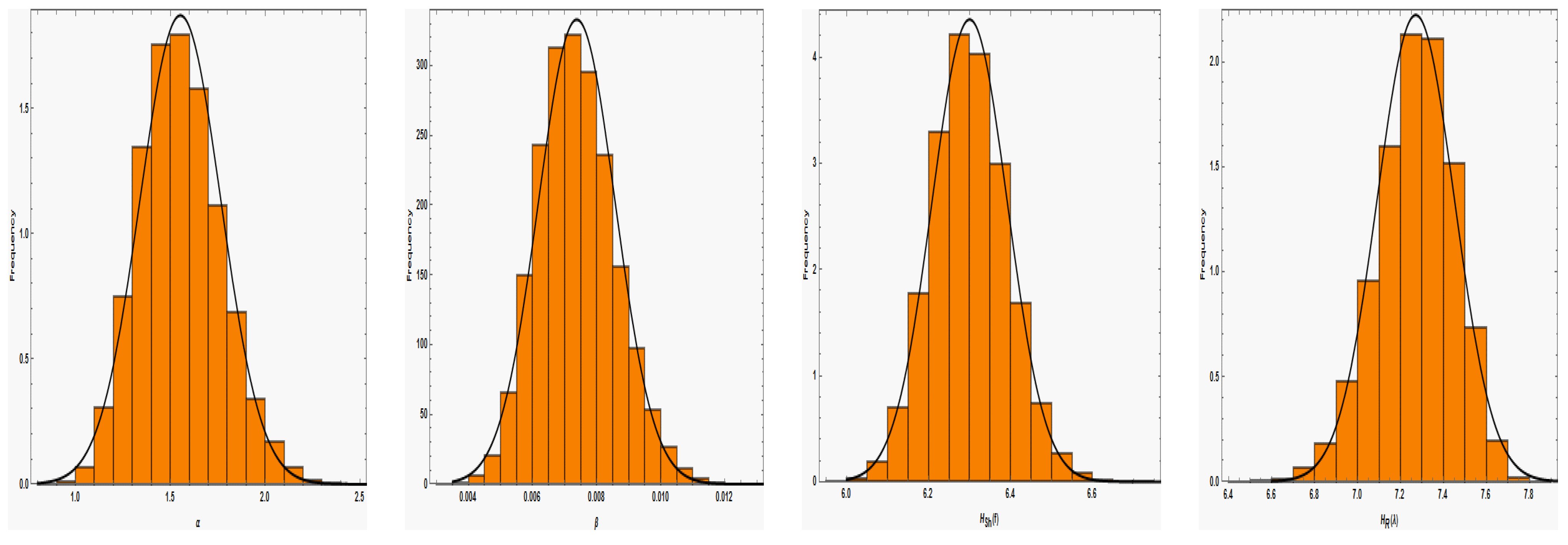Trace plots based on 60,000 chain values of $\alpha$, $\beta$, $H_{Sh}\left(f\right)$, and $H_R(\lambda =0.5)$ are provided in Figure 5 to demonstrate how well the simulated MCMC samples approximate. Each trace plot displays the sample’s arithmetic mean (represented by a dashed horizontal line) and its 95% HPD intervals (represented by a solid horizontal line). It shows that the MCMC method based on the remaining 60,000 variates converges successfully, and that using the first 10,000 samples as burn-in is suitable from a size point of view to eliminate the influence of the initial values. The histograms for the parameter estimates based on 60,000 chain values and the Gaussian kernel are also shown in Figure 6. The estimates unequivocally demonstrate that each and every one of the generated posteriors is symmetric with respect to the theoretical posterior density functions. The estimates clearly indicate that all of the generated posteriors are symmetric with respect to the theoretical posterior density functions.

In our next step, we randomly partition the given data into $n=44$ groups with $k=2$ independent items inside each group in order to analyze this data set using PFF censored samples. Thereafter, the following first-failure censored data are obtained: 8, 16, 16, 32, 40, 40, 56, 60, 72, 72, 72, 80, 80, 96, 108, 112, 120, 136, 152, 156, 168, 168, 168, 184, 184, 208, 216, 224, 224, 240, 256, 264, 280, 304, 328, 340, 358, 384, 400, 438, 464, 536, 576, 656. Next, we generate PFF censored samples using three different censoring schemes from the above first-failure censored sample with $m=30$. The different censoring schemes and the corresponding PFF censored samples are presented in

Table 2. PFF censored samples under the given censoring schemes when $k=2$, $n=44$, $m=30$.

Censoring Scheme	PFF Censored Samples
CS1 = (14, 0${}^{29}$)	8, 16, 16, 32, 40, 40, 56, 72, 72, 72, 80, 96, 108, 112, 136, 152, 168,
	168, 184, 216, 224, 240, 256, 264, 280, 304, 340, 358, 384, 438.
CS2 = (2, 0${}^5$, 2, 0${}^5$, 1, 0${}^7$)	8, 16, 16, 32, 40, 56, 72, 80, 80, 96, 108, 112, 120, 152, 156, 168, 184,
	184, 208, 216, 224, 256, 264, 280, 328, 340, 384, 400, 438, 536
CS3 = (0${}^{29}$, 14)	8, 16, 16, 32, 40, 40, 56, 60, 72, 72, 72, 80, 80, 96, 108, 112, 120, 136,
	152, 156, 168, 168, 168, 184, 184, 208, 216, 224, 224, 240.

. As was presented above for the complete sample, the estimates of ML and Bayes were calculated, and the numerical results are presented in

Table 3. Point and interval estimates of $\alpha$, $\beta$, $H_{Sh}\left(f\right)$, and $H_R(\lambda =0.5)$ from the real data.

Parameter			$\mathit{\alpha }$				$\mathit{\beta }$
Method		Schema	Estimate	Lower	Upper	Length	Estimate	Lower	Upper	Length
MLE	NR	Cs1	1.44313	0.98168	2.12149	1.13981	0.00496	0.00276	0.00890	0.00614
		Cs2	1.46065	0.99216	2.15035	1.15819	0.00358	0.00191	0.00673	0.00482
		Cs3	1.37690	0.91308	2.07633	1.16325	0.00371	0.00183	0.00750	0.00567
	EM	Cs1	1.44547	0.98308	2.12534	1.14226	0.00498	0.00277	0.00893	0.00616
		Cs2	1.46399	0.99416	2.15586	1.16170	0.00360	0.00192	0.00676	0.00484
		Cs3	1.38116	0.91546	2.08378	1.16832	0.00373	0.00184	0.00755	0.00571
Bayes	SEL	Cs1	1.54310	0.93542	2.91191	1.97649	0.00545	0.00239	0.01213	0.00974
		Cs2	1.43320	0.97454	2.08755	1.11301	0.00348	0.00168	0.00630	0.00462
		Cs3	1.34435	0.86997	1.90746	1.03749	0.00360	0.00155	0.00620	0.00465
Entropy			$H_{Sh}\left(f\right)$				$H_R(\lambda =0.5)$
MLE	NR	Cs1	6.63634	6.29810	6.99275	0.69465	7.52156	7.08909	7.98040	0.89131
		Cs2	6.97080	6.60485	7.35702	0.75217	7.87283	7.48185	8.28424	0.80239
		Cs3	6.88860	6.48434	7.31808	0.83374	7.70821	7.32243	8.11432	0.79189
	EM	Cs1	6.63434	6.29622	6.99063	0.69441	7.52182	7.08955	7.98045	0.89090
		Cs2	6.96789	6.60208	7.35398	0.75190	7.87311	7.48244	8.28417	0.80173
		Cs3	6.88480	6.48064	7.31415	0.83351	7.70873	7.32321	8.11455	0.79134
Bayes	SEL	Cs1	6.63101	6.21344	7.06922	0.85578	7.54058	7.04389	7.94138	0.89749
		Cs2	7.01253	6.64572	7.43173	0.78601	7.86092	7.46350	8.21397	0.75047
		Cs3	6.93107	6.56297	7.38494	0.82197	7.69129	7.26721	8.05765	0.79044

. Moreover, the estimates of $\alpha$, $\beta$, $H_{Sh}\left(f\right)$, and $H_R\left(\lambda \right)$ based on EM algorithm were calculated and added to the table because they differ from the estimates calculated by NR in the case of censored samples data.

Tabulated values show that the various estimations are reasonably close to one another. Moreover, for $\alpha$, $\beta$, and $H_R(\lambda =0.5)$, the Bayes estimation based on NIP has good behavior when compared to the other intervals in terms of interval lengths. In the cases of CS1 and CS2, we discover that the MLE of $H_{Sh}\left(f\right)$ based on the EM algorithm is the best estimate, whereas in the case of CS3, we find that the Bayes estimation based on the NIP prior is the best.

Table 4. Bayes estimates under LINEX loss function of $\alpha$, $\beta$, $H_{Sh}\left(f\right)$, and $H_R(\lambda =0.5)$.

	Scheme	$\mathit{\alpha }$	$\mathit{\beta }$	${\mathit{H}}_{\mathbf{Sh}}\left(\mathit{f}\right)$	${\mathit{H}}_{\mathit{R}}(\mathit{\lambda }=0.5)$
$v=-2$	Cs1	2.45503	0.005460	6.75540	7.65798
	Cs2	1.67847	0.003485	7.06924	7.94963
	Cs3	1.54419	0.003606	6.99635	7.78387
$v=+2$	Cs1	1.28181	0.005440	6.52537	7.38995
	Cs2	1.28098	1.280980	6.92419	7.75558
	Cs3	1.18843	0.003598	6.83454	7.57856

shows the effect of parameter v on the Bayes estimates, whereas in the case of negative values, we noticed that there was an increase in the values of the estimates from those calculated by the SE loss function, and vice versa in the case of the positive value. Practically, it is not possible to compare the methods presented in this paper with one sample, so we will present a simulation study in the next section.

6. Simulation Study

The proposed estimates of the entropy functions provided by (3) and (4), as well as the unknown parameters of the gamma distribution, are compared numerically in this section. Based on their average biases and mean squared errors (MSE), the MLEs and Bayes estimates are compared. On the other hand, for the interval estimates, we contrast them in light of their average lengths. For this aim, each simulation uses $N_s=1000$ PFF censored samples. The following steps were used to simulate a PFF-censored sample from the gamma distribution with parameters $\alpha$ and $\beta$ for given values of n, m, k, and a progressive censoring scheme $R=(R_1,\dots ,R_m)$:

(1)

Create a random sample of size m from standard uniform distribution, denoted by $W_1,\dots ,W_m$.

(2)

Set $V_i=W_i^{1/a_i}$ for $i=1,\dots ,m$ where $a_i=i+{\sum }_{j=m-i+1}^m{R}_j$.

(3)

Set $U_{i:m:n}^R=1-{\displaystyle \prod _{j=m-i+1}^m}{V}_i$ for $i=1,\dots ,m$. Thus, ($U_{1:m:n}^R,\dots ,U_{m:m:n}^R$) is a progressively Type-II censored sample from standard uniform distribution.

(4)

Set $Z_{i:m:n:k}^R=1-{(1-U_{i:m:n}^R)}^{1/k}$ for $i=1,\dots ,m$. The data set ($Z_{1:m:n:k}^R,\dots ,Z_{m:m:n:k}^R$) is a progressively first-failure censored sample from standard uniform distribution.

(5)

Finally, set $X_{1:m:n:k}^R=F^{-1}\left(Z_{i:m:n:k}^R\right)$ with $i=1,\dots ,m$, and hence, the required progressively first-failure censored sample is ($X_{1:m:n:k}^R,\dots ,X_{m:m:n:k}^R$).

Three different sample sizes, $n=20,30,$ and 50, as well as four failure sample sizes, $m=15,25$, and 40, were used in this study. Using different censoring schemes, we first derived progressively first-failure type-II censored samples that follow the gamma distribution with $\alpha =$$0.6$ and $\beta =1.5$. Then, we calculated the MLEs of $\alpha$, $\beta$, $H_{Sh}\left(f\right)$, and $H_R\left(\lambda \right)$ based on the NR method, using (10)–(15). Next, according to (35)–(38), the EM algorithm was applied to compute the MLEs. To compute the Bayes estimates based on the NIP and informative prior of $\alpha$ and $\beta$, using the MH algorithm, we ran the iterative process up to $N_{MC}=$ 11,000 iterations by discarding the first $M=1000$ iterations as a burn-in period. For the informative prior, the values of the hyperparameters were taken as $a=2.25$, $b=1.5$, $c=5.0$, and $d=5.0$. Moreover, the Bayes estimates with respect to the LINEX loss function were computed for the values of $v=-2.0$ and $v=+2.0$. Recall that the notation ($0^3,2$) used in the tables expresses the censoring scheme ($0,0,0,2$). The average bias values (in the first row) and the MSEs (in the second row) of the MLEs and Bayes estimates are presented in

Table 5. Average biases (first row) and MSEs (second row) of $\alpha$ when $\alpha =1.5$ and $\beta =1.0$.

$\mathit{k}=1$		MLE		Bayes under SE LF		Bayes Estimates under LINEX LF
						$v=-2.0$		$v=2.0$
(n,m)	Scheme	NR	EM	NIP	IP	NIP	IP	NIP	IP
$(30,16)$	$(16,0^{*15})$	0.412637	0.412232	0.188642	0.174476	0.209325	0.188521	0.180307	0.171575
		0.349373	0.34916	0.057631	0.048493	0.073109	0.058638	0.050423	0.045174
	$(0^{*13},16,0^{*2})$	0.474386	0.472699	0.158211	0.150584	0.169879	0.156888	0.156506	0.152586
		0.478504	0.477189	0.041775	0.036682	0.050048	0.041703	0.038517	0.035809
	$(0^{*15},16)$	0.485502	0.484135	0.159366	0.148991	0.174560	0.158257	0.153984	0.147972
		0.535746	0.534318	0.040305	0.034862	0.048944	0.040199	0.036791	0.033704
$(30,25)$	$(5,0^{*24})$	0.343223	0.343123	0.164589	0.157504	0.174713	0.164163	0.161352	0.157501
		0.220698	0.220670	0.043914	0.039751	0.050518	0.044294	0.041117	0.03859
	$(0^{*4},5,0^{*20})$	0.349521	0.349540	0.162824	0.155848	0.172143	0.162251	0.159314	0.154365
		0.239361	0.239347	0.041415	0.037344	0.047784	0.041822	0.038517	0.035973
	$(0^{*24},5)$	0.379232	0.379103	0.154932	0.148535	0.162951	0.153774	0.152049	0.148169
		0.286560	0.286428	0.037999	0.034463	0.043537	0.038253	0.035642	0.033479
$(60,35)$	$(25,0^{*34})$	0.245439	0.245116	0.129087	0.125357	0.134862	0.129177	0.127478	0.125676
		0.111697	0.111571	0.027347	0.025441	0.030537	0.027741	0.025873	0.024718
	$(0^{*24},25,0^{*35})$	0.270959	0.270125	0.114976	0.111474	0.119966	0.114911	0.112733	0.110562
		0.125865	0.125445	0.021508	0.020065	0.023577	0.021538	0.020471	0.019577
	$(0^{*34},25)$	0.288938	0.287722	0.115714	0.111634	0.121496	0.115885	0.112969	0.110111
		0.151141	0.150507	0.021435	0.019703	0.023709	0.021453	0.020125	0.018942
$(60,50)$	$(10,0^{*49})$	0.232288	0.232251	0.112970	0.109236	0.118591	0.113578	0.109782	0.107324
		0.095116	0.095094	0.020244	0.018807	0.022454	0.020523	0.018988	0.017992
	$(0^{*9},10,0^{*40})$	0.218645	0.218626	0.110894	0.107442	0.116380	0.111867	0.107718	0.105421
		0.086769	0.086756	0.019127	0.017944	0.020989	0.019393	0.018113	0.017283
	$(0^{*49},10)$	0.231342	0.231219	0.105253	0.102878	0.109103	0.105541	0.103849	0.102602
		0.093856	0.093776	0.017798	0.016867	0.019290	0.017977	0.017029	0.016473
$(100,80)$	$(20,0^{*79})$	0.174525	0.17445	0.088067	0.086913	0.089556	0.087845	0.087934	0.087392
		0.050900	0.05087	0.012678	0.012174	0.013276	0.012603	0.012428	0.012084
	$(0^{*19},20,0^{*60})$	0.167975	0.167908	0.088569	0.087382	0.089992	0.088238	0.088156	0.087368
		0.046918	0.046903	0.012093	0.011677	0.012537	0.011998	0.011919	0.011634
	$(0^{*79},20)$	0.167268	0.166912	0.079263	0.077797	0.080970	0.078999	0.078641	0.077602
		0.046477	0.046394	0.009983	0.009581	0.010451	0.009903	0.009796	0.009521
$\mathit{k}=\mathbf{2}$
$(30,16)$	$(16,0^{*15})$	0.369383	0.368708	0.158526	0.147502	0.174051	0.157661	0.151430	0.144355
		0.271727	0.270591	0.040433	0.034388	0.049361	0.040233	0.035542	0.032098
	$(0^{*13},16,0^{*2})$	0.418369	0.416682	0.135539	0.124952	0.148317	0.134080	0.127936	0.120555
		0.373192	0.369199	0.028792	0.024339	0.034880	0.028130	0.025889	0.022993
	$(0^{*15},16)$	0.474962	0.469911	0.133241	0.123647	0.146387	0.131280	0.127374	0.121860
		0.489678	0.483686	0.027948	0.023837	0.033825	0.027345	0.025247	0.022772
$(30,25)$	$(5,0^{*24})$	0.301205	0.300723	0.126295	0.120235	0.134232	0.125731	0.122184	0.118361
		0.165283	0.164639	0.025504	0.022969	0.029238	0.025551	0.023655	0.022057
	$(0^{*4},5,0^{*20})$	0.332598	0.332046	0.131107	0.123971	0.140715	0.131248	0.125472	0.120389
		0.216852	0.216110	0.028209	0.025096	0.032634	0.028329	0.025645	0.023482
	$(0^{*24},5)$	0.335533	0.334300	0.123607	0.117377	0.131147	0.122509	0.120143	0.115812
		0.213375	0.212197	0.024285	0.021717	0.027746	0.023982	0.022640	0.020919
$(60,35)$	$(25,0^{*34})$	0.254962	0.253487	0.110799	0.107448	0.115865	0.111038	0.108486	0.106148
		0.114289	0.113374	0.019054	0.017716	0.020939	0.019100	0.018029	0.017126
	$(0^{*24},25,0^{*35})$	0.237406	0.236031	0.092528	0.089157	0.096528	0.092168	0.090487	0.088283
		0.101323	0.099903	0.013314	0.012455	0.014571	0.013242	0.012852	0.012224
	$(0^{*34},25)$	0.268988	0.266251	0.094480	0.090518	0.098840	0.09384	0.092179	0.089179
		0.132578	0.130145	0.014072	0.012865	0.015532	0.01388	0.013291	0.012424
$(60,50)$	$(10,0^{*49})$	0.204982	0.204655	0.093533	0.091170	0.096236	0.092981	0.092409	0.090859
		0.074675	0.074306	0.013808	0.013053	0.014777	0.013671	0.013310	0.012855
	$(0^{*9},10,0^{*40})$	0.191604	0.191252	0.090974	0.088951	0.093890	0.091214	0.089358	0.087992
		0.063928	0.063613	0.012898	0.012250	0.013762	0.012875	0.012480	0.012014
	$(0^{*49},10)$	0.208836	0.207586	0.084197	0.082430	0.086559	0.083812	0.083412	0.082771
		0.075163	0.074463	0.011325	0.010757	0.012001	0.011213	0.011057	0.010668
$(100,80)$	$(20,0^{*79})$	0.153610	0.153411	0.070791	0.069413	0.072189	0.070437	0.070151	0.069288
		0.039458	0.039185	0.007999	0.007646	0.008319	0.007878	0.007846	0.007580
	$(0^{*19},20,0^{*60})$	0.147933	0.147076	0.068025	0.066757	0.069627	0.067903	0.067269	0.066379
		0.036153	0.035815	0.007502	0.007167	0.007840	0.007401	0.007354	0.007077
	$(0^{*79},20)$	0.161274	0.159672	0.065683	0.064504	0.066819	0.065205	0.065274	0.064609
		0.042841	0.042105	0.007013	0.006700	0.007243	0.006852	0.006929	0.006688

,

Table 6. Average biases (first row) and MSEs (second row) of $\beta$ when $\alpha =1.5$ and $\beta =1.0$.

$\mathit{k}=1$		MLE		Bayes under SE LF		Bayes Estimates under LINEX LF
						$v=-2.0$		$v=2.0$
(n,m)	Scheme	NR	EM	NIP	IP	NIP	IP	NIP	IP
$(30,16)$	$(16,0^{*15})$	0.370412	0.367898	0.103680	0.079863	0.143639	0.103777	0.087998	0.073615
		0.308440	0.306644	0.017209	0.009812	0.033506	0.017163	0.011815	0.008243
	$(0^{*13},16,0^{*2})$	0.502225	0.499371	0.100663	0.074011	0.148084	0.102548	0.084663	0.069586
		0.574257	0.57164	0.015751	0.008576	0.033450	0.015925	0.011390	0.007901
	$(0^{*15},16)$	0.505662	0.503348	0.091997	0.068022	0.139870	0.095786	0.079720	0.066547
		0.612167	0.609697	0.013462	0.007204	0.030228	0.014165	0.009972	0.006893
$(30,25)$	$(5,0^{*24})$	0.285854	0.285400	0.076571	0.064424	0.098364	0.079060	0.068925	0.061183
		0.160326	0.159988	0.009391	0.006477	0.015309	0.009774	0.007448	0.005842
	$(0^{*4},5,0^{*20})$	0.289206	0.289170	0.076964	0.063464	0.099979	0.078977	0.067947	0.060210
		0.169573	0.169495	0.009573	0.006499	0.015624	0.009822	0.007564	0.005859
	$(0^{*24},5)$	0.329083	0.328874	0.075802	0.063122	0.097536	0.077209	0.068438	0.060844
		0.213270	0.213121	0.008912	0.006155	0.014785	0.009283	0.007259	0.005783
$(60,35)$	$(25,0^{*34})$	0.210806	0.208874	0.064075	0.057201	0.075675	0.065201	0.060033	0.055835
		0.077889	0.076983	0.006584	0.005190	0.009078	0.006687	0.005860	0.005041
	$(0^{*24},25,0^{*35})$	0.261985	0.260595	0.065994	0.057782	0.080338	0.067934	0.061087	0.055865
		0.127576	0.126813	0.006851	0.005186	0.009867	0.007009	0.005986	0.004963
	$(0^{*34},25)$	0.278523	0.276683	0.061949	0.053626	0.077543	0.064291	0.056871	0.052037
		0.140232	0.139295	0.006048	0.004475	0.008997	0.006206	0.005322	0.004384
$(60,50)$	$(10,0^{*49})$	0.184433	0.184177	0.051875	0.047403	0.058689	0.052252	0.049569	0.046715
		0.061106	0.061032	0.004342	0.003575	0.005537	0.004353	0.003974	0.003477
	$(0^{*9},10,0^{*40})$	0.182036	0.181941	0.051155	0.046968	0.058495	0.052205	0.048771	0.046390
		0.060899	0.060846	0.004334	0.003539	0.005506	0.004390	0.003902	0.003391
	$(0^{*49},10)$	0.203301	0.203087	0.050648	0.046047	0.057738	0.051168	0.048649	0.045642
		0.073385	0.073289	0.004141	0.003308	0.005466	0.004171	0.003614	0.003189
$(100,80)$	$(20,0^{*79})$	0.141958	0.141579	0.041273	0.038742	0.045061	0.041495	0.039598	0.038054
		0.033414	0.033327	0.002752	0.002355	0.003241	0.002699	0.002568	0.002287
	$(0^{*19},20,0^{*60})$	0.140360	0.140176	0.041641	0.039409	0.044855	0.041659	0.040630	0.039240
		0.032386	0.03232	0.002756	0.002391	0.003198	0.002679	0.002642	0.002384
	$(0^{*79},20)$	0.146966	0.146473	0.037739	0.035601	0.041429	0.038296	0.037043	0.035721
		0.036945	0.036812	0.002347	0.002008	0.002783	0.002300	0.002263	0.002018
$\mathit{k}=\mathbf{2}$
$(30,16)$	$(16,0^{*15})$	0.397914	0.368708	0.158528	0.147502	0.174042	0.157661	0.151430	0.144355
		0.362548	0.270591	0.040435	0.034388	0.049354	0.040233	0.035936	0.032098
	$(0^{*13},16,0^{*2})$	0.538985	0.524034	0.103875	0.073213	0.156567	0.102607	0.088315	0.071065
		0.678709	0.663918	0.016776	0.008275	0.037460	0.016006	0.012632	0.008096
	$(0^{*15},16)$	0.613453	0.598226	0.104258	0.072357	0.163289	0.105232	0.086211	0.069542
		0.893110	0.875384	0.016768	0.008144	0.038846	0.016330	0.012176	0.007834
$(30,25)$	$(5,0^{*24})$	0.310024	0.307841	0.080950	0.066450	0.104377	0.081778	0.072761	0.063742
		0.179526	0.177978	0.010214	0.006822	0.016761	0.010287	0.008314	0.006343
	$(0^{*4},5,0^{*20})$	0.343865	0.341334	0.085301	0.069765	0.110537	0.086451	0.075416	0.065725
		0.249468	0.247684	0.011662	0.007659	0.019245	0.011719	0.008978	0.006734
	$(0^{*24},5)$	0.356477	0.353225	0.079019	0.063181	0.105374	0.080929	0.069327	0.059215
		0.262265	0.259929	0.009720	0.006160	0.016913	0.009979	0.007719	0.005652
$(60,35)$	$(25,0^{*34})$	0.257123	0.250115	0.072559	0.063537	0.085642	0.072820	0.067790	0.061164
		0.125380	0.122136	0.008448	0.006343	0.011810	0.008396	0.007279	0.005900
	$(0^{*24},25,0^{*35})$	0.283862	0.276155	0.069627	0.059083	0.085581	0.070064	0.064165	0.056991
		0.153539	0.149458	0.007570	0.005409	0.011387	0.007658	0.006465	0.005081
	$(0^{*34},25)$	0.32104	0.311534	0.065152	0.054676	0.084062	0.068291	0.058450	0.052634
		0.207647	0.201773	0.006749	0.004695	0.010871	0.007065	0.005501	0.004374
$(60,50)$	$(10,0^{*49})$	0.204335	0.202357	0.055409	0.049346	0.065054	0.056487	0.051228	0.047345
		0.077205	0.076256	0.004849	0.003796	0.006578	0.004965	0.004169	0.003470
	$(0^{*9},10,0^{*40})$	0.194780	0.191909	0.054219	0.049168	0.061566	0.054326	0.052405	0.049195
		0.069218	0.068157	0.004604	0.003805	0.006127	0.004729	0.004382	0.003704
	$(0^{*49},10)$	0.222347	0.219134	0.053958	0.048527	0.063065	0.055080	0.051111	0.047660
		0.088960	0.087423	0.004677	0.003692	0.006233	0.004712	0.004228	0.003576
$(100,80)$	$(20,0^{*79})$	0.151046	0.148006	0.042851	0.039935	0.046698	0.042597	0.041707	0.039768
		0.039129	0.038213	0.002989	0.002521	0.003551	0.002889	0.002815	0.002482
	$(0^{*19},20,0^{*60})$	0.157909	0.154323	0.045214	0.042480	0.049336	0.045608	0.043635	0.041567
		0.040398	0.039344	0.003175	0.002704	0.003805	0.003152	0.002936	0.002600
	$(0^{*79},20)$	0.175036	0.171054	0.043118	0.040201	0.047529	0.043507	0.041614	0.039685
		0.051506	0.049783	0.002947	0.002499	0.003557	0.002917	0.002755	0.002452

,

Table 7. Average biases (first row) and MSEs (second row) of $H_{Sh}\left(f\right)=1.3610$ when $\alpha =1.5$ and $\beta =1.0$.

$\mathit{k}=1$		MLE		Bayes under SE LF		Bayes Estimates under LINEX LF
						$v=-2.0$		$v=2.0$
(n,m)	Scheme	NR	EM	NIP	IP	NIP	IP	NIP	IP
$(30,16)$	$(16,0^{*15})$	0.180823	0.178393	0.131941	0.123177	0.131638	0.122395	0.145385	0.133168
		0.052639	0.051619	0.027957	0.024022	0.027053	0.023520	0.034591	0.028547
	$(0^{*13},16,0^{*2})$	0.221905	0.220477	0.117323	0.108250	0.117784	0.108479	0.129297	0.116068
		0.079219	0.078638	0.021714	0.018212	0.021477	0.018137	0.026886	0.021491
	$(0^{*15},16)$	0.217849	0.216710	0.110821	0.104003	0.114033	0.106038	0.120634	0.110441
		0.078300	0.077802	0.019509	0.016844	0.019958	0.017122	0.024151	0.019742
$(30,25)$	$(5,0^{*24})$	0.147138	0.146775	0.115755	0.110714	0.114380	0.109293	0.124289	0.117803
		0.034373	0.034204	0.021522	0.019594	0.020455	0.018732	0.025333	0.022571
	$(0^{*4},5,0^{*20})$	0.144625	0.144470	0.109671	0.105094	0.109167	0.104663	0.117749	0.111717
		0.033636	0.033596	0.019325	0.017527	0.018561	0.016974	0.022650	0.020079
	$(0^{*24},5)$	0.151344	0.151264	0.104831	0.100770	0.104436	0.100435	0.112630	0.106943
		0.036851	0.036823	0.017411	0.015891	0.016921	0.015557	0.020337	0.018082
$(60,35)$	$(25,0^{*34})$	0.120751	0.119033	0.095997	0.092558	0.095434	0.092219	0.100024	0.096073
		0.022249	0.021669	0.014350	0.013301	0.014386	0.013351	0.015653	0.014326
	$(0^{*24},25,0^{*35})$	0.137314	0.136494	0.083995	0.080954	0.085022	0.082178	0.087009	0.083065
		0.029859	0.029623	0.011166	0.010286	0.011253	0.010418	0.012144	0.011018
	$(0^{*34},25)$	0.138202	0.137270	0.077895	0.075218	0.079646	0.077281	0.079970	0.076593
		0.029926	0.029676	0.009487	0.008810	0.009790	0.009143	0.010261	0.009320
$(60,50)$	$(10,0^{*49})$	0.095924	0.095682	0.077378	0.075270	0.078435	0.076298	0.078950	0.076669
		0.014739	0.014674	0.009445	0.008851	0.009514	0.009026	0.009923	0.009241
	$(0^{*9},10,0^{*40})$	0.098920	0.098763	0.077231	0.075463	0.078035	0.076331	0.078995	0.076871
		0.015623	0.015594	0.009372	0.008928	0.009516	0.009007	0.009989	0.009386
	$(0^{*49},10)$	0.103651	0.103562	0.074475	0.072464	0.075414	0.073324	0.075916	0.073745
		0.017498	0.017475	0.008990	0.008380	0.008931	0.008385	0.009509	0.00888
$(100,80)$	$(20,0^{*79})$	0.075789	0.075436	0.061146	0.060246	0.061077	0.060239	0.062612	0.061561
		0.009043	0.008972	0.005987	0.005670	0.005829	0.005597	0.006301	0.005974
	$(0^{*19},20,0^{*60})$	0.078271	0.078037	0.060530	0.059618	0.060739	0.059884	0.061675	0.060508
		0.009589	0.009552	0.005811	0.005586	0.005817	0.005566	0.006124	0.00582
	$(0^{*79},20)$	0.079778	0.079549	0.055883	0.055111	0.056025	0.055285	0.056994	0.056168
		0.009909	0.009867	0.004978	0.004721	0.004993	0.004744	0.005181	0.004899
$\mathit{k}=\mathbf{2}$
$(30,16)$	$(16,0^{*15})$	0.197488	0.190905	0.113597	0.103656	0.118145	0.107073	0.122937	0.109979
		0.064322	0.062014	0.020763	0.017096	0.021900	0.018022	0.024328	0.019223
	$(0^{*13},16,0^{*2})$	0.253435	0.243632	0.101176	0.089468	0.111411	0.097988	0.106829	0.091902
		0.103449	0.099102	0.016554	0.012893	0.019120	0.014721	0.019250	0.014110
	$(0^{*15},16)$	0.272477	0.263248	0.095715	0.085353	0.103308	0.091114	0.106532	0.090900
		0.118072	0.113392	0.014889	0.01154	0.017035	0.013051	0.018023	0.013086
$(30,25)$	$(5,0^{*24})$	0.158762	0.156833	0.092156	0.086751	0.094015	0.088709	0.097210	0.090388
		0.039638	0.039084	0.013532	0.011877	0.013968	0.012348	0.015020	0.012925
	$(0^{*4},5,0^{*20})$	0.167019	0.165217	0.093280	0.087316	0.096109	0.090296	0.097162	0.089896
		0.046401	0.045814	0.014226	0.012430	0.014631	0.012949	0.015721	0.013395
	$(0^{*24},5)$	0.171199	0.168937	0.085547	0.080457	0.087996	0.082901	0.090796	0.084090
		0.047949	0.047276	0.012008	0.010496	0.012330	0.010842	0.013765	0.011616
$(60,35)$	$(25,0^{*34})$	0.134037	0.127955	0.078772	0.075069	0.080815	0.077244	0.081170	0.076638
		0.029500	0.027979	0.010231	0.009155	0.010466	0.009437	0.010982	0.009683
	$(0^{*24},25,0^{*35})$	0.155927	0.150187	0.071742	0.067423	0.072642	0.068757	0.075323	0.069888
		0.038117	0.036566	0.008268	0.007189	0.008485	0.007486	0.009025	0.007696
	$(0^{*34},25)$	0.166805	0.160208	0.068470	0.065093	0.070056	0.067051	0.071643	0.066844
		0.044306	0.042445	0.007291	0.006461	0.007553	0.006811	0.008087	0.006925
$(60,50)$	$(10,0^{*49})$	0.110864	0.108987	0.067342	0.064929	0.066405	0.064299	0.070539	0.067535
		0.019748	0.019371	0.007267	0.006672	0.007075	0.006599	0.007865	0.007170
	$(0^{*9},10,0^{*40})$	0.109931	0.107708	0.066317	0.064293	0.067142	0.065346	0.067947	0.065445
		0.019267	0.018773	0.006909	0.006407	0.006997	0.006563	0.007292	0.006671
	$(0^{*49},10)$	0.119926	0.117584	0.062125	0.059825	0.062340	0.060312	0.064499	0.061639
		0.022982	0.022454	0.006263	0.005742	0.006298	0.005833	0.006601	0.00607
$(100,80)$	$(20,0^{*79})$	0.084720	0.082083	0.051611	0.050287	0.052054	0.050933	0.052198	0.050651
		0.011458	0.011012	0.004387	0.004057	0.004322	0.004116	0.004512	0.004173
	$(0^{*19},20,0^{*60})$	0.091330	0.088686	0.052989	0.051720	0.053239	0.051995	0.053897	0.052465
		0.012737	0.012250	0.004471	0.004174	0.004486	0.004212	0.004658	0.004309
	$(0^{*79},20)$	0.098033	0.095225	0.049745	0.048399	0.049744	0.048705	0.050726	0.049196
		0.014851	0.014278	0.003928	0.003633	0.003929	0.003668	0.004011	0.003770

,

Table 8. Average biases (first row) and MSEs (second row) of $H_R(\lambda =0.25)=2.2768$ when $\alpha =1.5$ and $\beta =1.0$.

$\mathit{k}=1$		MLE		Bayes under SE LF		Bayes Estimates under LINEX LF
						$v=-2.0$		$v=2.0$
(n,m)	Scheme	NR	EM	NIP	IP	NIP	IP	NIP	IP
$(30,16)$	$(16,0^{*15})$	0.157642	0.155524	0.159521	0.150699	0.162387	0.152042	0.170578	0.159280
		0.039693	0.038757	0.040725	0.035981	0.041917	0.036978	0.046351	0.039985
	$(0^{*13},16,0^{*2})$	0.167950	0.167103	0.139632	0.131355	0.140709	0.132138	0.149141	0.138466
		0.044172	0.043854	0.030347	0.026807	0.030552	0.026995	0.035093	0.030020
	$(0^{*15},16)$	0.162464	0.161815	0.134261	0.128056	0.137378	0.130039	0.141485	0.133305
		0.041946	0.041682	0.027992	0.025263	0.028960	0.025877	0.031971	0.027980
$(30,25)$	$(5,0^{*24})$	0.136740	0.136417	0.142483	0.136956	0.142623	0.136522	0.149473	0.143425
		0.029888	0.029736	0.032019	0.029645	0.031811	0.029424	0.035570	0.032565
	$(0^{*4},5,0^{*20})$	0.133572	0.133464	0.136126	0.131615	0.136926	0.131691	0.142124	0.136822
		0.027591	0.027558	0.028938	0.026781	0.029035	0.026833	0.031915	0.029244
	$(0^{*24},5)$	0.130599	0.130571	0.129999	0.125590	0.130386	0.125821	0.136034	0.130918
		0.026513	0.026503	0.026154	0.024336	0.026285	0.024434	0.028837	0.026484
$(60,35)$	$(25,0^{*34})$	0.112513	0.110954	0.117248	0.113669	0.117567	0.113915	0.120682	0.116619
		0.019791	0.019251	0.021319	0.020067	0.021839	0.020489	0.022436	0.021017
	$(0^{*24},25,0^{*35})$	0.112773	0.112295	0.101387	0.098580	0.100296	0.102976	0.100721	0.103001
		0.020004	0.019873	0.016119	0.015261	0.015579	0.016356	0.016055	0.016899
	$(0^{*34},25)$	0.110207	0.109696	0.095291	0.092802	0.097244	0.094642	0.096586	0.094097
		0.018903	0.018779	0.014251	0.013536	0.014728	0.014015	0.014790	0.013934
$(60,50)$	$(10,0^{*49})$	0.091438	0.091211	0.096986	0.094525	0.098837	0.096249	0.097572	0.095193
		0.012818	0.012754	0.014557	0.013779	0.015116	0.014269	0.014840	0.014031
	$(0^{*9},10,0^{*40})$	0.092178	0.092071	0.096019	0.094043	0.097694	0.095475	0.096828	0.094903
		0.013207	0.013184	0.014380	0.013702	0.014733	0.014027	0.014789	0.014060
	$(0^{*49},10)$	0.091309	0.091272	0.092241	0.090046	0.093350	0.091038	0.093627	0.091589
		0.013306	0.013297	0.013571	0.012871	0.013698	0.013019	0.014017	0.013335
$(100,80)$	$(20,0^{*79})$	0.071913	0.071575	0.076425	0.075433	0.076505	0.075365	0.077711	0.076766
		0.008061	0.007992	0.009153	0.008817	0.009184	0.008797	0.009472	0.009142
	$(0^{*19},20,0^{*60})$	0.073279	0.073124	0.075169	0.074161	0.075482	0.074399	0.076014	0.075026
		0.008422	0.008394	0.008891	0.008585	0.008913	0.008600	0.009120	0.008835
	$(0^{*79},20)$	0.069697	0.069584	0.069347	0.068509	0.069782	0.068865	0.069936	0.069207
		0.007533	0.007512	0.007535	0.007252	0.007589	0.007309	0.007713	0.007434
$\mathit{k}=\mathbf{2}$
$(30,16)$	$(16,0^{*15})$	0.160725	0.155929	0.133151	0.125029	0.139100	0.129279	0.139388	0.129585
		0.041044	0.039258	0.028571	0.024997	0.030598	0.026478	0.031245	0.026703
	$(0^{*13},16,0^{*2})$	0.187853	0.180776	0.116003	0.106694	0.125722	0.114155	0.118357	0.108355
		0.056547	0.053498	0.021544	0.018351	0.024086	0.020155	0.023379	0.019259
	$(0^{*15},16)$	0.194993	0.188395	0.109839	0.102664	0.116556	0.107075	0.116384	0.106307
		0.059695	0.056516	0.019321	0.016569	0.021423	0.017983	0.021669	0.017840
$(30,25)$	$(5,0^{*24})$	0.127323	0.126074	0.109430	0.104942	0.112313	0.107288	0.112813	0.107557
		0.025550	0.025181	0.018995	0.017365	0.019817	0.018074	0.020224	0.018252
	$(0^{*4},5,0^{*20})$	0.131195	0.130022	0.109705	0.104811	0.113669	0.108539	0.112625	0.107043
		0.027973	0.027577	0.019983	0.018235	0.020881	0.019072	0.021018	0.018922
	$(0^{*24},5)$	0.129398	0.128019	0.102418	0.098424	0.104997	0.100791	0.105631	0.100999
		0.027409	0.027002	0.016951	0.015476	0.017236	0.015930	0.018290	0.016452
$(60,35)$	$(25,0^{*34})$	0.107708	0.103319	0.093129	0.090308	0.095489	0.092359	0.094722	0.091228
		0.018996	0.017856	0.014011	0.013023	0.014482	0.013432	0.014513	0.013445
	$(0^{*24},25,0^{*35})$	0.120417	0.116478	0.082141	0.078954	0.083246	0.080215	0.084688	0.080796
		0.022932	0.021887	0.010743	0.009827	0.011010	0.010096	0.011370	0.010268
	$(0^{*34},25)$	0.12587	0.121466	0.080398	0.077854	0.082009	0.079547	0.082011	0.078880
		0.024538	0.023393	0.009965	0.009229	0.010259	0.009567	0.010442	0.009585
$(60,50)$	$(10,0^{*49})$	0.092253	0.091083	0.080483	0.078610	0.079974	0.078181	0.083015	0.080793
		0.013431	0.013177	0.010326	0.009822	0.010230	0.009785	0.010935	0.010301
	$(0^{*9},10,0^{*40})$	0.092466	0.091007	0.079733	0.077946	0.080389	0.078887	0.080755	0.078579
		0.013280	0.012929	0.009819	0.009318	0.009992	0.009512	0.010112	0.009548
	$(0^{*49},10)$	0.094300	0.092846	0.073357	0.071538	0.073458	0.071821	0.075160	0.073046
		0.014138	0.013824	0.008636	0.008217	0.008784	0.008300	0.009006	0.008534
$(100,80)$	$(20,0^{*79})$	0.069869	0.068107	0.061345	0.060288	0.061834	0.060895	0.061775	0.060487
		0.007861	0.007545	0.006167	0.005853	0.006213	0.005926	0.006290	0.005960
	$(0^{*19},20,0^{*60})$	0.074736	0.072983	0.061955	0.060854	0.062217	0.061154	0.062579	0.061430
		0.008707	0.008366	0.006172	0.005875	0.006222	0.005925	0.006315	0.005994
	$(0^{*79},20)$	0.077352	0.075616	0.058399	0.057400	0.058423	0.057534	0.059199	0.058012
		0.009208	0.008876	0.005411	0.005131	0.005427	0.005155	0.005529	0.005267

and

Table 9. Average lengths (ALs) and coverage probabilities (CPs) of 95% confidence and credible intervals with ML and Bayes methods for $\alpha$, $\beta$, $H_{Sh}\left(f\right)$, and $H_R(\lambda =0.25)$, when $\alpha =1.5$, $\beta =1.0$, and $k=2$.

Parameter	n	m	Scheme	MLE NR		MLE EM		Bayes under NIP		Bayes under IP
				AL	CP	AL	CP	AL	CP	AL	CP
$\alpha$	30	16	$(14,{15}^0)$	2.01961	0.938	1.94581	0.932	0.94386	0.954	0.90951	0.963
			$(7^0,14,7^0)$	2.27650	0.917	2.28975	0.924	0.85113	0.959	0.81342	0.956
			$({15}^0,14)$	2.40506	0.923	2.41637	0.929	0.85574	0.964	0.81749	0.954
	30	25	$(10,{24}^0)$	1.67951	0.942	1.58507	0.929	0.79633	0.950	0.77431	0.947
			$({12}^0,{10}^1,{12}^0)$	1.65838	0.930	1.57494	0.949	0.77691	0.952	0.75826	0.949
			$({24}^0,10)$	1.78549	0.927	1.70788	0.934	0.76198	0.953	0.74274	0.953
	60	35	$(10,{34}^0)$	1.26690	0.943	1.19411	0.911	0.65642	0.959	0.64375	0.955
			$({17}^0,{10}^1,{17}^0)$	1.29433	0.950	1.27825	0.937	0.58705	0.956	0.57564	0.950
			$({34}^0,10)$	1.41520	0.935	1.39748	0.927	0.58831	0.958	0.57602	0.963
	60	50	$(10,{34}^0)$	1.12302	0.937	1.04105	0.926	0.56968	0.954	0.56186	0.961
			$({17}^0,{10}^1,{17}^0)$	1.08733	0.940	1.01990	0.924	0.55175	0.957	0.54349	0.954
			$({34}^0,10)$	1.15930	0.947	1.09731	0.914	0.54059	0.960	0.53280	0.960
	100	80	$(10,{34}^0)$	0.86093	0.943	0.79586	0.939	0.44869	0.952	0.44356	0.953
			$({17}^0,{10}^1,{17}^0)$	0.81576	0.951	0.76701	0.918	0.42745	0.957	0.42314	0.952
			$({34}^0,10)$	0.87953	0.96	0.83284	0.939	0.42102	0.961	0.41735	0.963
$\beta$	30	16	$(14,{15}^0)$	1.82788	0.925	1.82576	0.926	0.98201	0.959	0.85960	0.959
			$(7^0,14,7^0)$	2.50672	0.911	2.50337	0.912	1.04129	0.965	0.89729	0.967
			$({15}^0,14)$	2.64540	0.911	2.64333	0.911	1.04553	0.965	0.90126	0.958
	30	25	$(10,{24}^0)$	1.40378	0.931	1.40346	0.931	0.78894	0.976	0.72003	0.971
			$({12}^0,{10}^1,{12}^0)$	1.42220	0.925	1.42216	0.925	0.79174	0.971	0.72240	0.965
			$({24}^0,10)$	1.56931	0.924	1.56926	0.924	0.80251	0.972	0.72961	0.954
	60	35	$(10,{34}^0)$	1.07080	0.944	1.06986	0.945	0.65687	0.969	0.61414	0.950
			$({17}^0,{10}^1,{17}^0)$	1.28191	0.942	1.28153	0.943	0.68793	0.975	0.64138	0.957
			$({34}^0,10)$	1.40494	0.931	1.40444	0.932	0.69352	0.982	0.64725	0.961
	60	50	$(10,{34}^0)$	0.90327	0.933	0.90323	0.933	0.54608	0.980	0.52145	0.959
			$({17}^0,{10}^1,{17}^0)$	0.91046	0.932	0.91049	0.932	0.55095	0.975	0.52519	0.957
			$({34}^0,10)$	0.99687	0.944	0.99685	0.941	0.55979	0.965	0.53351	0.964
	100	80	$(10,{34}^0)$	0.69626	0.942	0.69625	0.942	0.43302	0.972	0.41887	0.957
			$({17}^0,{10}^1,{17}^0)$	0.69512	0.949	0.69515	0.949	0.43711	0.977	0.42100	0.963
			$({34}^0,10)$	0.76351	0.959	0.76350	0.960	0.44195	0.985	0.42950	0.961
$H_R\left(f\right)$	30	16	$(14,{15}^0)$	0.85760	0.955	0.85762	0.955	0.86236	0.986	0.77038	0.968
			$(7^0,14,7^0)$	1.00066	0.954	1.00064	0.954	0.88168	0.992	0.78292	0.957
			$({15}^0,14)$	1.02775	0.963	1.02770	0.963	0.88092	0.991	0.78974	0.962
	30	25	$(10,{24}^0)$	0.68058	0.955	0.68058	0.956	0.69387	0.987	0.65715	0.956
			$({12}^0,{10}^1,{12}^0)$	0.68509	0.943	0.68425	0.943	0.69669	0.989	0.66902	0.960
			$({24}^0,10)$	0.70677	0.944	0.70676	0.944	0.73649	0.990	0.68796	0.958
	60	35	$(10,{34}^0)$	0.57528	0.961	0.57530	0.962	0.60780	0.989	0.53822	0.960
			$({17}^0,{10}^1,{17}^0)$	0.63645	0.945	0.63643	0.945	0.59823	0.987	0.55682	0.962
			$({34}^0,10)$	0.66504	0.959	0.66502	0.959	0.59372	0.988	0.56849	0.966
	60	50	$(10,{34}^0)$	0.47735	0.948	0.47735	0.949	0.50754	0.990	0.43981	0.963
			$({17}^0,{10}^1,{17}^0)$	0.48190	0.956	0.48189	0.956	0.51472	0.992	0.46292	0.959
			$({34}^0,10)$	0.49621	0.941	0.49620	0.941	0.52046	0.989	0.49574	0.965
	100	80	$(10,{34}^0)$	0.37705	0.956	0.37701	0.957	0.31739	0.992	0.30783	0.963
			$({17}^0,{10}^1,{17}^0)$	0.38386	0.956	0.38382	0.956	0.40098	0.991	0.37992	0.954
			$({34}^0,10)$	0.39670	0.958	0.39669	0.958	0.40257	0.990	0.39402	0.966
$H_{SH}\left(f\right)$	30	16	$(14,{15}^0)$	0.84631	0.966	0.78509	0.943	0.85662	0.978	0.76396	0.953
			$(7^0,14,7^0)$	0.98099	0.984	0.77736	0.92	0.88389	0.981	0.75380	0.962
			$({15}^0,14)$	1.00673	0.989	0.78075	0.929	0.79948	0.985	0.74984	0.957
	30	25	$(10,{24}^0)$	0.67533	0.941	0.64093	0.928	0.70392	0.977	0.61010	0.953
			$({12}^0,{10}^1,{12}^0)$	0.67966	0.954	0.63127	0.937	0.64911	0.973	0.60646	0.958
			$({24}^0,10)$	0.70088	0.966	0.62015	0.933	0.67072	0.978	0.58698	0.951
	60	35	$(10,{34}^0)$	0.57234	0.961	0.54413	0.944	0.56605	0.977	0.53014	0.965
			$({17}^0,{10}^1,{17}^0)$	0.63233	0.977	0.52616	0.934	0.55622	0.975	0.51036	0.961
			$({34}^0,10)$	0.66036	0.985	0.52689	0.935	0.54764	0.980	0.47168	0.952
	60	50	$(10,{34}^0)$	0.47571	0.961	0.45594	0.955	0.46652	0.973	0.44975	0.958
			$({17}^0,{10}^1,{17}^0)$	0.48019	0.970	0.44937	0.953	0.45312	0.981	0.40745	0.952
			$({34}^0,10)$	0.49433	0.966	0.44103	0.940	0.53960	0.969	0.39351	0.964
	100	80	$(10,{34}^0)$	0.37624	0.966	0.36217	0.957	0.34857	0.976	0.33972	0.954
			$({17}^0,{10}^1,{17}^0)$	0.38305	0.964	0.35660	0.945	0.43464	0.975	0.32496	0.952
			$({34}^0,10)$	0.39576	0.974	0.34973	0.956	0.42073	0.979	0.31320	0.963

. The bias and mean-squared errors (MSEs) of the estimates were computed using the following formula:

$$bias=\frac{1}{N_s}\sum _{i=1}^{N_s}\left({\widehat{\Theta }}_l^{\left(i\right)}-{\Theta }_l\right),\mathrm{and}MSE=\frac{1}{N_s}\sum _{i=1}^{N_s}{\left({\widehat{\Theta }}_l^{\left(i\right)}-{\Theta }_l\right)}^2,l=1,2,3,4.$$

For the problem under study, ${\Theta }_1=\alpha ,{\Theta }_2=\beta ,{\Theta }_3=H_{Sh}\left(f\right),{\Theta }_4=H_R\left(\lambda \right)$, and $N=1000$.

Besides the point estimates, log-transformed MLEs, EM, and Bayesian methods were used to obtain the 95% confidence/credible intervals for $\alpha$, $\beta$, $H_{Sh}\left(f\right)$, and $H_R(\lambda =0.25)$. Table 9 and

Table 10. Average lengths (ALs) and coverage probabilities (CPs) of 95% confidence and credible intervals with ML and Bayes methods for $\alpha$, $\beta$, $H_{Sh}\left(f\right)$, and $H_R(\lambda =0.25)$, when $\alpha =1.5$, $\beta =1.0$, and $k=2$.

Parameter	n	m	Scheme	MLE NR		MLE EM		Bayes NIP		Bayes IP
				AL	CP	AL	CP	AL	CP	AL	CP
$\alpha$	30	16	$(14,{15}^0)$	1.78674	0.941	1.81981	0.947	0.81676	0.962	0.77612	0.966
			$(7^0,14,7^0)$	2.03198	0.937	2.15737	0.975	0.76213	0.968	0.71471	0.977
			$({15}^0,14)$	2.21356	0.924	2.35594	0.969	0.76755	0.981	0.71533	0.979
	30	25	$(10,{24}^0)$	1.48399	0.938	1.48753	0.940	0.67463	0.970	0.65415	0.969
			$({12}^0,{10}^1,{12}^0)$	1.49320	0.914	1.50844	0.928	0.66649	0.962	0.64542	0.962
			$({24}^0,10)$	1.60100	0.932	1.63256	0.941	0.65766	0.964	0.63415	0.966
	60	35	$(10,{34}^0)$	1.15108	0.93	1.16022	0.932	0.55911	0.967	0.54389	0.968
			$({17}^0,{10}^1,{17}^0)$	1.16061	0.947	1.23157	0.970	0.51605	0.972	0.50081	0.974
			$({34}^0,10)$	1.30330	0.944	1.38474	0.976	0.52341	0.965	0.50373	0.973
	60	50	$(10,{34}^0)$	1.00051	0.947	1.00062	0.945	0.47653	0.963	0.46755	0.960
			$({17}^0,{10}^1,{17}^0)$	0.95478	0.944	0.96339	0.949	0.46821	0.959	0.45850	0.961
			$({34}^0,10)$	1.03529	0.954	1.05504	0.961	0.46211	0.972	0.45327	0.971
	100	80	$(10,{34}^0)$	0.76210	0.943	0.75925	0.947	0.37812	0.964	0.37266	0.971
			$({17}^0,{10}^1,{17}^0)$	0.73355	0.959	0.74406	0.961	0.36421	0.966	0.35996	0.959
			$({34}^0,10)$	0.79786	0.957	0.81699	0.963	0.36388	0.961	0.35692	0.965
$\beta$	30	16	$(14,{15}^0)$	2.03506	0.932	2.02946	0.933	1.02891	0.959	0.88643	0.965
			$(7^0,14,7^0)$	2.84353	0.913	2.82815	0.913	1.09653	0.955	0.92837	0.967
			$({15}^0,14)$	3.17284	0.911	3.15695	0.913	1.11588	0.969	0.94093	0.962
	30	25	$(10,{24}^0)$	1.55736	0.936	1.55674	0.936	0.81921	0.966	0.74405	0.961
			$({12}^0,{10}^1,{12}^0)$	1.60933	0.911	1.60834	0.911	0.82769	0.964	0.74918	0.964
			$({24}^0,10)$	1.79698	0.927	1.79577	0.928	0.84377	0.961	0.76282	0.959
	60	35	$(10,{34}^0)$	1.21326	0.917	1.21189	0.919	0.68819	0.957	0.64040	0.967
			$({17}^0,{10}^1,{17}^0)$	1.43795	0.943	1.43579	0.946	0.72710	0.968	0.67163	0.960
			$({34}^0,10)$	1.64605	0.938	1.64323	0.939	0.74342	0.967	0.68362	0.955
	60	50	$(10,{34}^0)$	1.02248	0.942	1.02164	0.943	0.57931	0.963	0.54930	0.963
			$({17}^0,{10}^1,{17}^0)$	0.99959	0.948	0.99930	0.948	0.57723	0.957	0.54783	0.966
			$({34}^0,10)$	1.12165	0.942	1.12062	0.944	0.59082	0.962	0.58946	0.971
	100	80	$(10,{34}^0)$	0.76420	0.942	0.76407	0.944	0.45351	0.963	0.56049	0.963
			$({17}^0,{10}^1,{17}^0)$	0.77187	0.953	0.77118	0.956	0.45732	0.967	0.44234	0.962
			$({34}^0,10)$	0.86484	0.940	0.86363	0.942	0.46892	0.962	0.45195	0.961
$H_R\left(f\right)$	30	16	$(14,{15}^0)$	0.95421	0.952	0.95420	0.955	0.86987	0.966	0.77516	0.967
			$(7^0,14,7^0)$	1.21093	0.983	1.21061	0.983	0.88422	0.968	0.77104	0.965
			$({15}^0,14)$	1.26910	0.987	1.26870	0.988	0.88928	0.975	0.77344	0.971
	30	25	$(10,{24}^0)$	0.76157	0.962	0.70158	0.996	0.70356	0.977	0.65205	0.974
			$({12}^0,{10}^1,{12}^0)$	0.76814	0.941	0.76813	0.943	0.69874	0.981	0.64830	0.975
			$({24}^0,10)$	0.82651	0.958	0.82647	0.959	0.69965	0.974	0.64722	0.977
	60	35	$(10,{34}^0)$	0.63906	0.945	0.63905	0.946	0.59023	0.978	0.55752	0.980
			$({17}^0,{10}^1,{17}^0)$	0.74830	0.961	0.74827	0.963	0.59298	0.975	0.55530	0.974
			$({34}^0,10)$	0.80973	0.958	0.80969	0.959	0.59583	0.971	0.55671	0.975
	60	50	$(10,{34}^0)$	0.53478	0.958	0.53480	0.958	0.49489	0.980	0.47602	0.973
			$({17}^0,{10}^1,{17}^0)$	0.54373	0.954	0.54372	0.955	0.49369	0.979	0.47302	0.971
			$({34}^0,10)$	0.58288	0.953	0.58288	0.953	0.49322	0.984	0.47303	0.976
	100	80	$(10,{34}^0)$	0.42191	0.981	0.35317	0.943	0.39251	0.983	0.38388	0.982
			$({17}^0,{10}^1,{17}^0)$	0.43228	0.955	0.43230	0.96	0.38743	0.982	0.37819	0.977
			$({34}^0,10)$	0.46835	0.947	0.46836	0.952	0.38912	0.989	0.38069	0.971
$H_{SH}\left(f\right)$	30	16	$(14,{15}^0)$	0.93855	0.986	0.77955	0.933	0.86601	0.988	0.76662	0.978
			$(7^0,14,7^0)$	1.17480	0.989	0.90007	0.930	0.84425	0.991	0.75143	0.993
			$({15}^0,14)$	1.22601	0.993	0.92475	0.917	0.84781	0.990	0.75127	0.990
	30	25	$(10,{24}^0)$	0.75433	0.984	0.62307	0.946	0.70563	0.986	0.60353	0.986
			$({12}^0,{10}^1,{12}^0)$	0.76042	0.975	0.61937	0.918	0.69744	0.984	0.65547	0.979
			$({24}^0,10)$	0.81681	0.988	0.63857	0.938	0.69078	0.989	0.64647	0.988
	60	35	$(10,{34}^0)$	0.63494	0.978	0.53164	0.944	0.59103	0.987	0.51356	0.985
			$({17}^0,{10}^1,{17}^0)$	0.74148	0.983	0.58497	0.938	0.57021	0.992	0.54034	0.990
			$({34}^0,10)$	0.80086	0.991	0.60912	0.943	0.56822	0.993	0.53678	0.995
	60	50	$(10,{34}^0)$	0.53238	0.978	0.44181	0.941	0.49749	0.991	0.48198	0.983
			$({17}^0,{10}^1,{17}^0)$	0.54127	0.985	0.44911	0.951	0.49280	0.992	0.47577	0.989
			$({34}^0,10)$	0.57981	0.987	0.46081	0.949	0.48534	0.990	0.46949	0.989
	100	80	$(10,{34}^0)$	0.42191	0.981	0.35317	0.943	0.39266	0.981	0.38388	0.982
			$({17}^0,{10}^1,{17}^0)$	0.43106	0.981	0.35685	0.959	0.38605	0.982	0.37807	0.985
			$({34}^0,10)$	0.46680	0.987	0.37032	0.947	0.38213	0.987	0.37220	0.989

give the average lengths (ALs) and coverage probabilities (CPs) of the resulting intervals of $\alpha$, $\beta$, $H_{Sh}\left(f\right)$, and $H_R(\lambda =0.25)$ with $k=1,2$, respectively. In general, we notice from Table 6, Table 7, Table 8 and Table 9 that the Bayes estimates have superior performance compared to the MLEs in terms of the MSEs. For the case of the LINEX loss function, the Bayes estimate of $\alpha$ and $\beta$ seems to be a reasonable choice when $v=2$. However, the best choice of $H_{Sh}\left(f\right)$, and $H_R(\lambda =0.25)$ is when $v=-2$. Additionally, it was found that the Bayes estimates derived using the informative prior (IP) perform better in terms of MSEs than those acquired using the NIP. Furthermore, the average biases and MSEs both tend to decrease with increasing effective sampling sizes. As a result, increasing the sample size generally yields better-estimating results. Moreover, in most cases considered, the MSEs of all estimates decrease as k increases, while n and m remain fixed. The ALs of the NIP are also longer than IP ALs. Then, the IP outperforms the NIP. Table 9 and Table 10 show that for all censoring schemes, the EM technique produces more precise confidence intervals than NR intervals. Comparing all three methods, it is evident that Bayes credible intervals have the best average lengths. Then, the Bayes approach is more suited to obtaining the confidence intervals of $\alpha$, $\beta$, $H_{Sh}\left(f\right)$, and $H_R\left(\lambda \right)$. Additionally, compared to the IP, the NIP ALs have greater lengths. Then, the IP outperforms the NIP. Finally, it can be noted that all average interval lengths decrease when the effective sample sizes increase. Moreover, it was observed that the CPs of the asymptotic and credible intervals of $\alpha$, $\beta$, $H_{Sh}\left(f\right)$, and $H_R(\lambda =0.25)$ were all close to the desired level of 0.95.

7. Conclusions

To date, many mindsets have developed different methods of information measurement to explore information in a hazy environment, and researchers are still working hard to develop such information measures that are more reliable, accurate, and reasonably useful with current measurement techniques. One of these methods is the study of entropy functions. In this paper, the entropy of the gamma distribution was investigated and estimated by the classical and Bayesian approach. When the provided data are progressively first-failure Type-II censored, the point and interval estimations of the unknown gamma distribution parameters are produced using the maximum likelihood and Bayesian estimations. The MLEs of the model parameters and entropy indices were created here using the NR and EM processes. To construct CIs for the unknown parameters and entropy indexes, the log transformation method was developed. It was found that this approach is better than the direct asymptotic normal technique. The EM algorithm is also considered to derive the interval estimates of the unknown parameters as well as the Shannon and Rényi entropies. Meanwhile, CIs for entropy indexes have also been provided, along with the delta technique. The EM estimates have the smallest root MSE and interval lengths when compared with those based on the NR method. We also considered the Bayes estimates of the unknowns and associated credible intervals. The Bayesian estimates were obtained using the MCMC method based on both symmetric and asymmetric loss functions, including the squared error and LINEX loss functions. The effectiveness of the various proposed estimators was assessed and contrasted using Monte Carlo simulations and a real-world application case. The Bayesian estimates with informative prior under LINEX loss function are the best among all estimates, according to the simulation analysis in this paper. In addition, when compared to alternative CIs, the Bayes credible intervals consistently have the lowest interval length.

The feature of the proposed work makes it easier for decision makers to deal with the ambiguity that arises due to neutral variables in complex cases, as well as in the case of censored data. Although many studies have theoretically investigated the properties of the gamma distribution, there is still a serious lack of statistical tools dedicated to facilitating their practical applications to be studied in the future, such as predictions and accelerated life tests. In this paper, very important and recent applied data (radio transceiver data) that had not been used before in statistical inference were used, and we expect that these data will be used in many research papers in the near future in the field of various life tests and statistical predictions. The following issue may be a topic for further investigation in the next paper:

“Objective Bayesian analysis for the differential entropy of the two parameter Gamma distribution based on progressively type-II censored samples: Informative and non-informative priors”.

References

1. Lawless, J.F. Statistical Models and Methods for Lifetime Data; John Wiley & Sons: Hoboken, NJ, USA, 2011. [Google Scholar]
2. Son, Y.S.; Oh, M. Bayesian estimation of the two-parameter Gamma distribution. Commun. Stat. Simul. Comput. 2006, 35, 285–293. [Google Scholar] [CrossRef]
3. Pradhan, B.; Kundu, D. Bayes estimation and prediction of the two-parameter gamma distribution. J. Stat. Simul. 2011, 81, 1187–1198. [Google Scholar] [CrossRef]
4. Basak, I.; Balakrishnan, N. Estimation for the three-parameter gamma distribution based on progressively censored data. Stat. Methodol. 2012, 9, 305–319. [Google Scholar] [CrossRef]
5. de Almeida, M.H.; Ramos, P.L.; Rao, G.S.; Moala, F.A. Objective Bayesian inference for the capability index of the Gamma distribution. Qual. Reliab. Eng. Int. 2021, 37, 2235–2247. [Google Scholar] [CrossRef]
6. Dey, S.; Elshahhat, A.; Nassar, M. Analysis of progressive type-II censored gamma distribution. Comput. Stat. 2023, 38, 481–508. [Google Scholar] [CrossRef]
7. Singh, V.P. Entropy Theory and Its Application in Environmental and Water Engineering; John Wiley & Sons: Hoboken, NJ, USA, 2013. [Google Scholar]
8. Rényi, A. On measures of entropy and information. In Proceedings of the Fourth Berkeley Symposium on Mathematical Statistics and Probability, Volume 1: Contributions to the Theory of Statistics, Davis, CA, USA, 30 June–30 July 1960; University of California Press: Oakland, CA, USA, 1961; Volume 4, pp. 547–562. [Google Scholar]
9. Amigó, J.M.; Balogh, S.G.; Hernández, S. A brief review of generalized entropies. Entropy 2018, 20, 813. [Google Scholar] [CrossRef]
10. Shannon, C.E. A mathematical theory of communication. Bell Syst. Tech. J. 1948, 27, 379–423. [Google Scholar] [CrossRef]
11. Acharya, J.; Orlitsky, A.; Suresh, A.T.; Tyagi, H. Estimating Rényi entropy of discrete distributions. IEEE Trans. Inf. Theory 2016, 63, 38–56. [Google Scholar] [CrossRef]
12. Cornforth, D.J.; Tarvainen, M.P.; Jelinek, H.F. Using renyi entropy to detect early cardiac autonomic neuropathy. In Proceedings of the 2013 35th Annual International Conference of the IEEE Engineering in Medicine and Biology Society (EMBC), Osaka, Japan, 3–7 July 2013; IEEE: Piscataway, NJ, USA; pp. 5562–5565. [Google Scholar]
13. Kang, S.B.; Cho, Y.S.; Han, J.T.; Kim, J. An estimation of the entropy for a double exponential distribution based on multiply Type-II censored samples. Entropy 2012, 14, 161–173. [Google Scholar] [CrossRef]
14. Cho, Y.; Sun, H.; Lee, K. An estimation of the entropy for a Rayleigh distribution based on doubly-generalized Type-II hybrid censored samples. Entropy 2014, 16, 3655–3669. [Google Scholar] [CrossRef]
15. Cho, Y.; Sun, H.; Lee, K. Estimating the entropy of a Weibull distribution under generalized progressive hybrid censoring. Entropy 2015, 17, 102–122. [Google Scholar] [CrossRef]
16. Chacko, M. Estimation of entropy for generalized exponential distribution based on record values. J. Indian Soc. Probab. Stat. 2018, 19, 79–96. [Google Scholar] [CrossRef]
17. Liu, S.; Gui, W. Estimating the entropy for Lomax distribution based on generalized progressively hybrid censoring. Symmetry 2019, 11, 1219. [Google Scholar] [CrossRef]
18. Yu, J.; Gui, W.; Shan, Y. Statistical inference on the Shannon entropy of inverse Weibull distribution under the progressive first-failure censoring. Entropy 2019, 21, 1209. [Google Scholar] [CrossRef]
19. Balakrishnan, N.; Aggarwala, R. Progressive Censoring: Theory, Methods, and Applications; Springer Science & Business Media: Berlin/Heidelberg, Germany, 2000. [Google Scholar]
20. Wu, S.J.; Kuş, C. On estimation based on progressive first-failure-censored sampling. Comput. Stat. Data Anal. 2009, 53, 3659–3670. [Google Scholar] [CrossRef]
21. Dube, M.; Krishna, H.; Garg, R. Generalized inverted exponential distribution under progressive first-failure censoring. J. Stat. Comput. Simul. 2016, 86, 1095–1114. [Google Scholar] [CrossRef]
22. Maurya, R.K.; Tripathi, Y.M.; Rastogi, M.K. Estimation and prediction for a progressively first-failure censored inverted exponentiated Rayleigh distribution. J. Stat. Theory Pract. 2019, 13, 1–48. [Google Scholar] [CrossRef]
23. Mathai, A.M. A Handbook of Generalized Special Functions for Statistical and Physical Sciences; Oxford University Press: New York, NY, USA, 1993. [Google Scholar]
24. Askey, R.A.; Daalhuis, A.B.O. Generalized Hypergeometric Functions and Meijer G-Function; Cambridge University Press: Cambridge, UK, 2010. [Google Scholar]
25. Meeker, W.Q.; Escobar, L.A. Statistical Methods for Reliability Data; John Wiley and Sons, Inc.: Hoboken, NJ, USA, 1998. [Google Scholar]
26. Dempster, A.P.; Laird, N.M.; Rubin, D.B. Maximum likelihood from incomplete data via the EM algorithm. J. R. Stat. Soc. Ser. B (Methodol.) 1977, 39, 1–22. [Google Scholar]
27. Ng, H.K.T.; Chan, P.S.; Balakrishnan, N. Estimation of parameters from progressively censored data using EM algorithm. Comput. Stat. Data Anal. 2002, 39, 371–386. [Google Scholar] [CrossRef]
28. McLachlan, G.J.; Krishnan, T. The EM Algorithm and Extensions; John Wiley & Sons: Hoboken, NJ, USA, 2007. [Google Scholar]
29. Louis, T.A. Finding the observed information matrix when using the EM algorithm. J. R. Stat. Ser. B (Methodol.) 1982, 44, 226–233. [Google Scholar]
30. Zhuang, L.; Xu, A.; Wang, X. A prognostic driven predictive maintenance framework based on Bayesian deep learning. Reliab. Eng. Syst. Saf. 2023, 234, 109181. [Google Scholar] [CrossRef]
31. Luo, C.; Shen, L.; Xu, A. Modelling and estimation of system reliability under dynamic operating environments and lifetime ordering constraints. Reliab. Eng. Syst. Saf. 2022, 218, 108136. [Google Scholar] [CrossRef]
32. Qin, S.; Wang, B.; Wu, W.; Ma, C. The prediction intervals of remaining useful life based on constant stress accelerated life test data. Eur. J. Oper. Res. 2022, 301, 47–755. [Google Scholar] [CrossRef]
33. Varian, H.R. A Bayesian approach to real estate assessment. In Studies in Bayesian Econometric and Statistics in Honor of Leonard J; Savage: Brule, WI, USA, 1975; pp. 195–208. [Google Scholar]
34. Geman, S.; Geman, D. Stochastic relaxation, Gibbs distributions, and the Bayesian restoration of images. IEEE Trans. Pattern Anal. Mach. Intell. 1984, PAMI-6, 721–741. [Google Scholar] [CrossRef] [PubMed]
35. Hastings, W.K. Monte Carlo sampling methods using Markov chains and their applications. Biometrika 1970, 57, 97–109. [Google Scholar] [CrossRef]
36. Aitkin, M. Introduction to Statistical Modelling and Inference; CRC Press: Boca Raton, FL, USA, 2022. [Google Scholar]
37. Geweke, J.F. Evaluating the Accuracy of Sampling-Based Approaches to the Calculation of Posterior Moments (No. 148); Federal Reserve Bank of Minneapolis: Minneapolis, MN, USA, 1991. [Google Scholar]
Figure 1. Parametric and nonparametric plots of radio transceiver data.
Mathematics 11 02298 g001
Figure 2. The 3D plot of the observed log-likelihood function of radio transceiver data.
Mathematics 11 02298 g002
Figure 3. Contour plot of the log-likelihood function for two parameters α , β under radio transceiver data.
Mathematics 11 02298 g003
Figure 4. The profile log-likelihood functions for each parameter. The vertical lines signify the MLEs α ^ = 1.538 and β ^ = 0.0073 . (a) The profile log-likelihood for α ; (b) the profile log-likelihood for β .
Mathematics 11 02298 g004
Figure 5. Trace MCMC plots for radio transceiver data.
Mathematics 11 02298 g005
Figure 6. Histograms with estimated kernel density of α , β , H S h ( f ) , and H R ( λ ) under radio transceiver data.
Mathematics 11 02298 g006