Article

Adaptive Finite/Fixed Time Control Design for a Class of Nonholonomic Systems with Disturbances

1
Grenoble Alpes University, CNRS, Grenoble INP, GIPSA-Lab, 38000 Grenoble, France
2
Department of Computer & Network Engineering, College of Computer Science and Engineering, University of Jeddah, Jeddah 21959, Saudi Arabia
3
Department of Cybersecurity, College of Computer Science and Engineering, University of Jeddah, Jeddah 21959, Saudi Arabia
*
Author to whom correspondence should be addressed.
Mathematics 2023, 11(10), 2287; https://doi.org/10.3390/math11102287
Submission received: 11 April 2023 / Revised: 24 April 2023 / Accepted: 5 May 2023 / Published: 14 May 2023
(This article belongs to the Special Issue Advances in Intelligent Control)

Abstract

:
This paper addresses the fixed-time stability analysis of a mobile unicycle-like system (UTMS) with chained shape dynamics (CFD) and subjected to unknown matched uncertainties. To achieve fixed-time stabilization of a nonholonomic (NS) system in CFD, an adaptive nonsingular fast terminal sliding mode control scheme (ANFTSMC) is proposed. To determine the upper bounds of the disturbances, only velocity and position measurements are required. In addition, the control rule uses the Lyapunov theory, which guarantees the stability of the closed-loop system. To emphasize/evaluate the efficacy of the proposed method, simulations are performed in different disturbance situations.

1. Introduction

The fourth industrial revolution ushered in a surge of change that encompassed logistics. Transportation has been one of the most pressing issues since the dawn of human civilization. Several applications for various activities may be identified, all aimed at efficiently improving processes and, as a result, production and volume [1]. Some collaborative robots in logistics applications can even be taught to perform tasks. This cuts down on wasteful programming time and improves the bespoke packaging process’s speed. Robots are increasingly infiltrating the logistics and transportation industries [1].
Mobile robots are becoming increasingly used in real-world applications, such as material handling, logistics, warehouses and last-mile delivery. Although they are flexible, this class of dynamic systems may face several issues when used in real indoor (Figure 1) or outdoor (Figure 2) applications. Mobile robots’ issues may include modeling, control, identification, as well as cybersecurity, particularly when used in outdoor applications. With the increased reliance on robotics, cybersecurity is vital to prevent threats that can have devastating effects, such as the loss of human lives in some applications, including medicine or firefighting, etc. Most threats in robotics applications stem from robotics communications [2]. This is due to the large volume of messages often exchanged over the internet, an insecure network by default, between the nodes themselves or with the cloud. Hence, it is crucial to have efficient security measures to protect from likely attacks, such as unauthorized access, malware, denial of service (DoS), eavesdropping, man-in-the-middle attacks (MITM), spoofing, and service hijacking [3]. However, more efforts are needed to improve [2]: (1) the quality of service (QoS) and quality of control (QoC) in the often-distributed robotics, (2) the overall reliability of wireless links and latency, (3) the data security, especially while in transit, (4) the autonomous cognitive decisions based on data exchanged in networks, and (5) the lightweight anomalies detection and prevention in real time to isolate and/or suspend affected components. Therefore, security must be considered during the design of robotic systems (security-by-design) as part of the safety requirements, not just as an added layer.
From the control perspective, mobile robots are sensitive to disturbances that may affect their behavior. For this reason, the design of a robust controller becomes a must. In this paper, we will concentrate on control issues.
Due to its practical significance in areas, such as mobile robotics (MR), wheeled vehicles (WV), submersible vehicles (SV), and satellites, NS control has garnered a lot of attention in recent decades [4,5]. However, because the number of input signals is smaller than the number of degrees of freedom, managing such systems difficult. Because of the non integrable limitations, controlling this type of system poses substantial difficulty. Smooth state feedback control methods cannot stabilize this type of system at an equilibrium point. The constructive control approaches are discontinuous control techniques based on two pats. These robots are controlled by these strategies, unlike continuous approaches. In this context, we present some constructive control approaches, such as adaptive fuzzy velocity field control [6], discontinuous feedback [7,8], hybrid feedback [9], and smooth time-varying feedback [10,11]. These approaches have been proposed to address this problem. Many advances in the stabilization of NSs have been made as a result of these effective approaches. For example, in [12], the authors proposed two strategies for the same system studied in our paper; the first approach used is state scaling and the second is the back stepping technique with adaptive laws in its design. Muñoz-Vázquez et al. [6] developed a control strategy for systems based on a changing supply rater and switching control. Unlike in [12,13], where asymptotic convergence was provided in these techniques, our proposed strategy is based on fixed-time control providing a fixed-time convergence of the first state system, and using a non-linear sliding manifold, the second state subsystem converges to zero in a finite-time. In addition, the second proposed controller uses adaptive law to cope with the upper bound of disturbances.
It is worth noting that the vast majority of existing references are concerned with the system trajectory’s asymptotic behavior, which means that the stable equilibrium point is reached as time approaches infinity [14]. Nonetheless, many applications expect control system trajectories to converge to an interesting equilibrium in short finite-time (FT) [14]. Furthermore, FT stable systems typically exhibit a number of desirable characteristics, including disturbance rejection, faster convergence, and improved robustness. In recent years, there has been a lot of interest in the research on FT stabilization of NSs [14].
As a result, research into nonholonomic system finite-time stabilization has gained a lot of interest in recent years. The authors of [15] proposed a simple adaptive control technique with actuator dynamics for trajectory-tracking of uncertain NSs. All kinematics, dynamics, and actuator dynamics parameters are assumed to be unknown. For a category of NSs with CFD, the fixed-time and the predefined-time stabilization problem are investigated, respectively, in [15,16,17,18]. The work developed in [19] explores fixed-time stabilization utilizing output feedback for CFD. A contour tracking scheme with a dynamic controller for uncertain nonholonomic systems based on an adaptive velocity field formulation was proposed in [20]. A new adaptive technique is proposed in [21] that ensures that the control torque bounds are computed in advance as a result of only the design parameters and desired trajectories.
According to Polyakov in [22], fixed-time stability is a novel approach that has recently been presented to create algorithms that ensure that the settling-time is upper bounded regardless of the start conditions. This concept is promising, since it allows one to build a controller capable of achieving specified control performances in a specific period of time and regardless of the start conditions. In this case, unlike the finite-time controllers, there is no need to fine-tune the design control parameters to maintain the settling time. Fixed-time stability is a new technique that has recently been proposed to develop algorithms that guarantee that the settling time is upper bounded independent of the start conditions [22]. This notion is promising, since it allows one to construct a controller that can achieve certain control performances in a specific amount of time and regardless of the start conditions. Unlike finite-time controllers, there is no need to fine-tune the design control settings to preserve the settling time in this scenario.
Motivated by the above observations, the current work proposes a new adaptive nonsingular fast TSMC approach for the fixed control of a nonholonomic robot system. This approach eliminates the singularity problem in TSMC and reduces the chattering phenomenon in SMC. The following are the paper’s key contributions:
  • For the first time, the fixed-time stability problem of a nonholonomic system is addressed inside the considered system’s unified framework, with and without output limitations;
  • New control approach for the second-order systems of a mobile robot is designed to achieve the fixed-time stability in the presence of external disturbances;
  • The upper-bound of perturbations is addressed using an on-line estimation based on adaptive control laws;
  • Simulation results using various scenarios in terms of disturbances are carried out in order to validate the theoretical findings of the suggested control strategy.
The following is the remainder of this paper: Section 2 explains some basics on the fixed-/finite-time stability and the main equations of the NS with RCD. The results are presented in Section 3. The first step is to offer a control signal for the stabilizing of the Z 0 ( t ) -subsystem with matched perturbations. The second step is to design an adaptive NFTSMC scheme for the second-order systems with matched perturbations. Following this, a switching strategy is presented based on the new results for the UTMS. Three scenarios are considered in the simulations, which are presented in Section 4. This paper concludes with Section 5.

2. Preliminaries and Conceptualization of the Problem

2.1. Preliminary Considerations for the Finite-/Fixed-Time Stability

Taking the system provided below:
Z ˙ ( t ) = Ψ ( Z ; Φ )
where Z ( t ) R n denotes the state variable of the system. The notation Φ is the constant parameter of system (1). The function Ψ ( Z ; Φ ) : R n R n is nonlinear, and the origin is considered to be a system (1) equilibrium point. Its initial conditions are Z 0 = Z ( 0 ) R n .
Definition 1
([22,23]). If there is such a thing as a function Φ T : R n R + , (1) its origin is a globally finite-time stable. So that the solution Ψ ( t , Z 0 ) of system (1) reaches the point of equilibrium in a certain amount of time. So, the setting time function can be defined for t [ 0 , Ψ ( Z 0 ) ] , for t Φ T ( Z 0 ) , a n d Ψ ( Z 0 , t ) = 0 .
Definition 2
([22,23]). It is a global fixed-time equilibrium if system (1) is worldwide finite-time stable and the settling-time expression Φ T ( Z 0 is limited by a positive value Φ T M a x > 0 .
Lemmas 1 and 2 are employed to explain the finite-time stability in the face of rapid time convergence.
Lemma 1
([24]). Consider the term φ ( t ) as the Lyapunov function (LF) presented as follows:
φ ( t ) μ b φ ( t ) μ c φ ς ( t ) , t 0 , φ ( t 0 ) 0
where, μ b > 0 , μ c > 0 , φ 0 is the initial value of φ ( t ) , 0 < ς < 1 . Let us consider φ ( t ) , t > t 1 , after a simple calculation, the t s is
t s = t 0 + 1 μ b ( 1 ς ) l n μ b φ 1 ς ( t 0 ) + μ c μ c
Lemma 2
([25]). Consider the Lyapunov function φ ( t ) with the initial value φ 0 as
φ ( t ) μ b φ ( t ) , t 0 , φ ( t 0 ) 0
where μ b > 0 , 0 < ς < 1 . Let us consider φ ( t ) , t > t 1 .
Then, the corresponding settling time t s can be given as
t r t 0 + μ b φ 1 ς ( t 0 ) ν a ( 1 ς )

2.2. Formulation of the Problem

Consider an MR that rides a unicycle, as shown in Figure 3. It contains two driving wheels that are individually operated by two actuators, as well as one passive wheel that prevents the plane from flipping over, when it is moving. The mass center’s position ( x ( t ) , y ( t ) ) is located at the junction of a straight line traveling through the robot’s center and the axes of the two driving wheels. The configuration of this MR is given as:
X ( t ) = [ x ( t ) y ( t ) θ ( t ) ] T ,
The term θ ( t ) represents the heading angle of this MR. The non slipping conditions and the pure rolling are given by the following equation.
S θ ( t ) x ˙ ( t ) C θ ( t ) ) y ˙ ( t ) = 0 .
The notations C z / S z are, respectively, cos z / sin z . The kinematics of the wheeled MR under the nonholonomic constraints can be defined as:
x ˙ ( t ) =   C θ ( t ) ν ( t ) y ˙ ( t ) =   S θ ( t ) ν ( t ) θ ˙ ( t ) =   ω ( t )
The notations ω ( t ) / ν ( t ) represent, respectively, the angular/linear velocities.
Let us introduce the following change.
Z 0 ( t ) =   x ( t ) Z 2 ( t ) =   y ( t ) Z 3 ( t ) =   tan ( θ ( t ) ) U 0 ( t ) =   ν ( t ) C θ ( t ) U 1 ( t ) =   ω ( t ) sec 2 ( θ ( t ) )
Using the transformation, system (7) can be described as:
Z ˙ 0 ( t )   = U 0 ( t ) + D 0 ( t ) Z ˙ 1 ( t )   = U 0 ( t ) Z 2 ( t ) Z ˙ 2 ( t )   = U 1 ( t ) + D 1 ( t )
where D 0 ( t ) and D 1 ( t ) are unknown perturbations.

3. Main Results

A constructive technique is presented in this section for the design of the FT stabilizer of (9) in the presence of perturbations, for any amount of time T > 0 given. We begin by selecting an acceptable non-zero constant input A 0 for U 0 ( t ) . As a result, the Z ( t ) -subsystem may be regarded as a non-linear control, for which the fixed-time stabilizing controller was developed. Once U 0 ( t ) reaches zero before a specified time and remains at zero, we design a new controller U 0 ( t ) to fixed-time stabilize the Z 0 ( t ) -subsystem.

3.1. Stabilization of the Z 0 ( t ) -Subsystem with Matched Perturbation

In this section, the fixed-time stabilization of a single CFD is presented. A single CFD’s fixed-time stability is ensured by the switching controller provided in the following theorem.
Proposition 1.
Consider Z 0 ( t ) -subsystem with the switched control scheme given by:
U 0 ( t ) = A 0 i f t T 1 c 0 | Z 0 ( t ) | α 1 s i g n ( Z 0 ( t ) ) c 1 | Z 0 ( t ) | α 2 s i g n ( Z 0 ( t ) ) c 2 s i g n ( Z 0 ( t ) )
where c i is a positive constant. Then, the Z 0 ( t ) -subsystem is fixed-time stable.
Proof. 
The LF candidate is considered as:
V 0 ( t ) = 1 2 Z 0 2 ( t )
Differencing V 0 ( t ) as:
V ˙ 0 ( t ) = c 0 | Z 0 ( t ) | α 1 + 1 c 1 | Z 0 ( t ) | α 2 + 2 c 2 | Z 0 ( t ) ) |
c 0 ( 2 V 0 ( t ) ) α 1 + 1 2 c 1 ( 2 V 0 ( t ) ) α 2 + 1 2 c 2 ( 2 V 0 ( t ) ) 1 2
Based on Lemma 2, the Z 0 ( t ) -subsystem is fixed-time stable. □
In this subsection, a simple controller is designed to stabilize the first-order system with matched perturbations. In the following subsection, a new control approach will be designed for second-order systems under matched perturbations.

3.2. Stabilization of the Second System with Disturbances

  • Stabilization of the second system based on NFTSMC method.
The design procedure for the control input U 1 ( t ) for the second MR system will be presented in this section. Let us consider the second-order system subjected to uncertainties and disturbances as:
Z ˙ 1 ( t ) =   Z 2 ( t ) Z ˙ 2 ( t ) =   Δ P ( Z ) + D 1 ( t ) + U 1 ( 1 )
with
| D 1 ( t ) | =   | ( Δ P ( Z ) + D 1 ( t ) ) |   δ 1
where δ 1 is the uncertainty/disturbance upper bound. The expression for δ 1 is as [26,27,28,29]:
δ 1 = d 0 + d 1 | Z 1 ( t ) | + d 2 | Z 2 ( t ) |
where d 0 , d 1 , and d 2 are positive constants.
Let us introduce the sliding variable as [26,27,30]:
σ ( t ) = Z 1 ( t ) + b | Z 1 ( t ) | β 2 s i g n ( Z 1 ( t ) ) + a | Z 1 ˙ ( t ) | β 1 s i g n ( Z 1 ˙ ( t ) )
where b and a are positive constants, 1 < β 1 < 2 and β 2 > β 1 . The time-derivative of the sliding variable is
σ ˙ ( t ) = Z 2 ( t ) + β 2 b | Z 1 ( t ) | β 2 1 Z 2 ( t ) + β 1 a | Z 2 ( t ) | β 1 1 ( U 1 ( t ) )
The analogous law may be obtained by setting σ ˙ ( t ) = 0
U e q 1 ( t ) = ( 1 β 1 a | Z 2 ( t ) | 2 β 1 ( 1 + β 2 b | Z 1 ( t ) | β 2 1 ) s i g n ( Z 2 ( t ) ) )
To reject the disturbances and establish resilience against their impacts on the mobile robot’s second system, the switching control law (SCL) U 1 ( t ) = h 1 σ ( t ) K 1 s i n g ( σ ( t ) ) is added to (19), where h 1 and K 1 are the switching gains. According to [31], the appropriate value of K 1 is K 1 = δ 1 + h 2 , where h 2 is a positive parameter.
The SCL is modified as:
U 1 ( t ) = h 1 σ ( t ) ( d 0 + d 1 | Z 1 ( t ) | + d 2 | Z 2 ( t ) | + h 2 ) s i n g ( σ ( t ) ) .
As a result, the SCL for second MR order system is
U s w 1 ( t ) = ( h 1 σ ( t ) K 1 s i g n ( σ ( t ) ) ) = ( h 1 σ ( t ) ( δ 1 + h 2 ) s i g n ( σ ( t ) ) ) = ( h 1 σ ( t ) ( d 0 + d 1 | Z 1 ( t ) | + d 2 | Z 2 ( t ) | + h 2 ) s i g n ( σ ( t ) ) )
As a result, the control law for the second-order system of the MR is as follows:
U 1 ( t ) = U s w 1 ( t ) + U e q 1 ( t ) = ( h 1 σ ( t ) ( d 0 + d 1 | Z 1 ( t ) | + d 2 | Z 2 ( t ) | + h 2 ) s i g n ( σ ( t ) ) 1 β 1 a | Z 2 ( t ) | 2 β 1 ( 1 + β 2 b | Z 1 ( t ) | β 2 1 ) s i g n ( Z 2 ( t ) ) )
Theorem 1.
Consider the second-order system of the MR presented in (14) and the sliding variable designed in (17) with the control scheme developed in (21), then the state Z 1 ( t ) and Z 2 ( t ) converge to σ ( t ) in a FT t r , then the global FT of the original system is stable.
Proof. 
To prove Theorem 1, the LF candidate is chosen as:
V 1 ( t ) = 0.5 σ 2 ( t )
Differencing V 1 ( t ) as:
V ˙ 1 ( t ) = σ ˙ ( t ) σ ( t ) = σ ( t ) ( Z 2 ( t ) + β 2 b | Z 1 ( t ) | β 2 1 Z 2 ( t ) + β 1 a | Z 2 ( t ) | β 1 1 Z ˙ 2 ( t ) )
By substituting (21) into (23), the dynamic of V 1 ( t ) becomes:
V ˙ 1 ( t ) = β 1 a | Z 2 ( t ) | β 1 1 ( D 1 ( t ) σ ( t ) h 1 σ 2 ( t ) ( δ 1 + h 2 ) | σ ( t ) | ) β 1 a | Z 2 ( t ) | β 1 1 ( | ( D 1 ( t ) | . | σ ( t ) | h 1 σ ( t ) 2 ( δ 1 + h 2 ) | σ ( t ) | ) = β 1 a | Z 2 ( t ) | β 1 1 ( | ( D 1 ( t ) | δ 1 ) | σ ( t ) | h 1 σ ( t ) 2 h 2 | σ ( t ) | )
Using Equation (15), we have
V ˙ 1 ( t ) β 1 a | Z 2 ( t ) | β 1 1 ( h 1 σ 2 ( t ) h 2 | σ ( t ) | ) 0
Equation (24) ensures that the stability criterion is met. The system’s state variables converge to σ ( t ) = 0 asymptotically. To demonstrate the existence of this convergence, Equation (25) can be expressed as:
V ˙ 1 ( t ) d V 1 ( t ) d t 2 β 1 a h 1 | Z 2 ( t ) | β 1 1 V 1 ( t ) 2 β 1 a h 2 | Z 2 ( t ) | β 1 1 V 1 1 / 2 ( t )
By defining 0 = 2 β 1 a h 1 | Z 2 ( t ) | β 1 1 and 1 = 2 β 1 a h 2 | Z 2 ( t ) | β 1 1 , it results in:
d V 1 ( t ) d t 0 V 1 ( t ) 1 V 1 1 / 2 ( t )
Following some calculations, we have
d t d V 1 ( t ) 0 V 1 ( t ) + 1 V 1 1 / 2 ( t ) = d V 1 1 / 2 ( t ) 0 V 1 ( t ) + 1
Now, integrating (28) from t 0 into t r , we can obtain
t r t 0 + 2 0 ln ( 0 V 1 1 / 2 ( t 0 ) + 1 1 )
This completes the proof above. □
  • Stabilization of the second system based on the adaptive NFTSMC (ANFTSMC) method.
The adaptive NFTSMC method was developed to determine the unknown δ 1 affecting the second-order system of the mobile robot. As a result, the position’s control signals are adjusted as follows:
U 1 ( t ) = U s w 1 ( t ) + U e q 1 ( t ) = ( h 1 σ ( t ) ( d ^ 0 + d ^ 1 | Z 1 ( t ) | + d ^ 2 | Z 2 ( t ) | + h 2 ) s i g n ( σ ( t ) ) 1 β 1 a | Z 2 ( t ) | 2 β 1 ( 1 + β 2 b | Z 1 ( t ) | β 2 1 ) s i g n ( Z 2 ( t ) ) )
where d ^ 0 , d ^ 1 , and d ^ 2 are the estimates of d 0 , d 1 , and d 2 , respectively.
The parameters d ^ 0 , d ^ 1 , and d ^ 2 are amended by the adaptive laws.
d ^ ˙ 0 = μ 0 | σ ( t ) | . | Z 2 ( t ) | β 1 1
d ^ ˙ 1 = μ 1 | σ ( t ) | . | Z 1 ( t ) | . | Z 2 ( t ) | β 1 1
d ^ ˙ 2 = μ 2 | σ ( t ) | . | Z 2 ( t ) | β 1
where μ 0 , μ 1 , and μ 2 are positive constants.
Theorem 2.
Consider the system (14) and the sliding variable designed in (17) with the control scheme developed in (21) and the adaptive laws (31)–(33), hence, the states Z 1 ( t ) and Z 2 ( t ) converge to σ ( t ) in a FT t r , then the global finite-time of the original of system is stable.
Proof. 
In order to determine the expressions of the parameters ( d ^ 0 , d ^ 1 , d ^ 2 ) and to demonstrate the RM’s second-order stability, the LF candidate is
V 1 ( t ) = 1 2 σ 2 ( t ) + β 1 a i = 0 2 1 2 μ i ( d ^ i d i ) 2
The time-derivative of Equation (34) is
V ˙ 1 ( t ) = σ ˙ ( t ) σ ( t ) + β 1 a i = 0 2 1 μ i ( d ^ i d i ) d ^ ˙ i
According to Equation (18), we can obtain
V ˙ 1 ( t ) = σ ( t ) ( Z 2 ( t ) + β 2 b | Z 1 ( t ) | β 2 1 Z 2 ( t ) + β 1 a | Z 2 ( t ) | β 1 1 Z ˙ 2 ( t ) + β 1 a i = 0 2 1 μ i ( d ^ i d i ) d ^ ˙ i
Using Equation (30), the dynamic of V 1 ( t ) is
V 1 ( t ) = β 1 a | Z 2 ( t ) | β 1 1 ( D 1 ( t ) σ ( t ) h 1 σ 2 ( t ) ( d ^ 0 + d ^ 1 | Z 1 ( t ) | + d ^ 2 | Z 2 ( t ) | + h 2 ) | σ ( t ) | ) + β 1 a i = 0 2 1 μ i ( d ^ i d i ) d ^ ˙ i
Using Equations (31)–(33), we can obtain
V 1 ( t ) = β 1 a | Z 2 ( t ) | β 1 1 ( D 1 ( t ) σ ( t ) h 2 | σ ( t ) | h 1 σ 2 ( t ) ( d ^ 0 + d ^ 1 | Z 1 ( t ) | + d ^ 2 | Z 2 ( t ) | ) | σ ( t ) | )
Based on (15), we obtain
V ˙ 1 ( t ) β 1 a | Z 2 ( t ) | β 1 1 ( | ( D 1 ( t ) | . | σ ( t ) | h 2 | σ ( t ) | h 1 σ ( t ) 2 ( d 0 + d 1 | Z 1 ( t ) | d 2 | Z 2 ( t ) | ) | σ ( t ) | ) β 1 a | Z 2 ( t ) | β 1 1 ( h 2 | σ ( t ) | h 1 σ ( t ) 2 ) 0
The Lyapunov equation V ˙ 1 ( t ) 0 ensures that the state variables of the second-order of the mobile robot converge in a FT to zero.
Moreover, according to the nonsingular terminal sliding surface proposed in [30], the sliding surface establishes the fast finite-time convergence of states ( x 1 , x 2 ) to zero.

3.3. Stabilization of Nonholonomic Chained-Form Systems with Unknown Perturbations

Based on the prior conclusions for first- and second-order subsystems, the switching approach is used in the following theorem to ensure fixed-time stability of the closed-loop system for uncertain NSs with CFD in the presence of disturbances.
Theorem 3.
For the system (9), use the following switching controller
U 0 ( t ) = A 0 i f t T 1 c 0 | Z 0 ( t ) | α 1 s i g n ( Z 0 ( t ) ) c 1 | Z 0 ( t ) | α 2 s i g n ( Z 0 ( t ) ) c 2 s i g n ( Z 0 ( t ) )
U 1 ( t ) = ( h 1 σ ( t ) ( d ^ 0 + d ^ 1 | Z 1 ( t ) | + d ^ 2 | Z 2 ( t ) | + h 2 ) s i g n ( σ ( t ) ) 1 β 1 a | Z 2 ( t ) | 2 β 1 ( 1 + β 2 b | Z 1 ( t ) | β 2 1 ) s i g n ( Z 2 ( t ) ) ) i f t T 1 K 2 s i g n ( Z 2 ( t ) )
where K 2 is a positive constant.
The closed-loop system (9) becomes fixed-time stable as a result.
Proof. 
In order to prove the above Theorem 3, two parts will be defined.
(1)
For t T 1 , U 0 ( t ) = A 0 ( t ) is used as a constant control input. Then, in the presence of, one may deduce that Z 1 ( t ) and Z 2 ( t ) converge to zero in the fixed-time T 1 based on the result of Theorem 2.
(2)
For t T 1 , the control signal U 1 ( t ) is developed to drive Z 2 ( t ) = 0 . Consider the LF candidate V 2 ( t ) = | Z 2 ( t ) | and its time-derivative as V ˙ 2 ( t ) | Z 2 ( t ) | ( K 2 δ 1 ) . We chose K 2 > δ 1 , then the Z 2 ( t ) = 0 for all t T 1 .

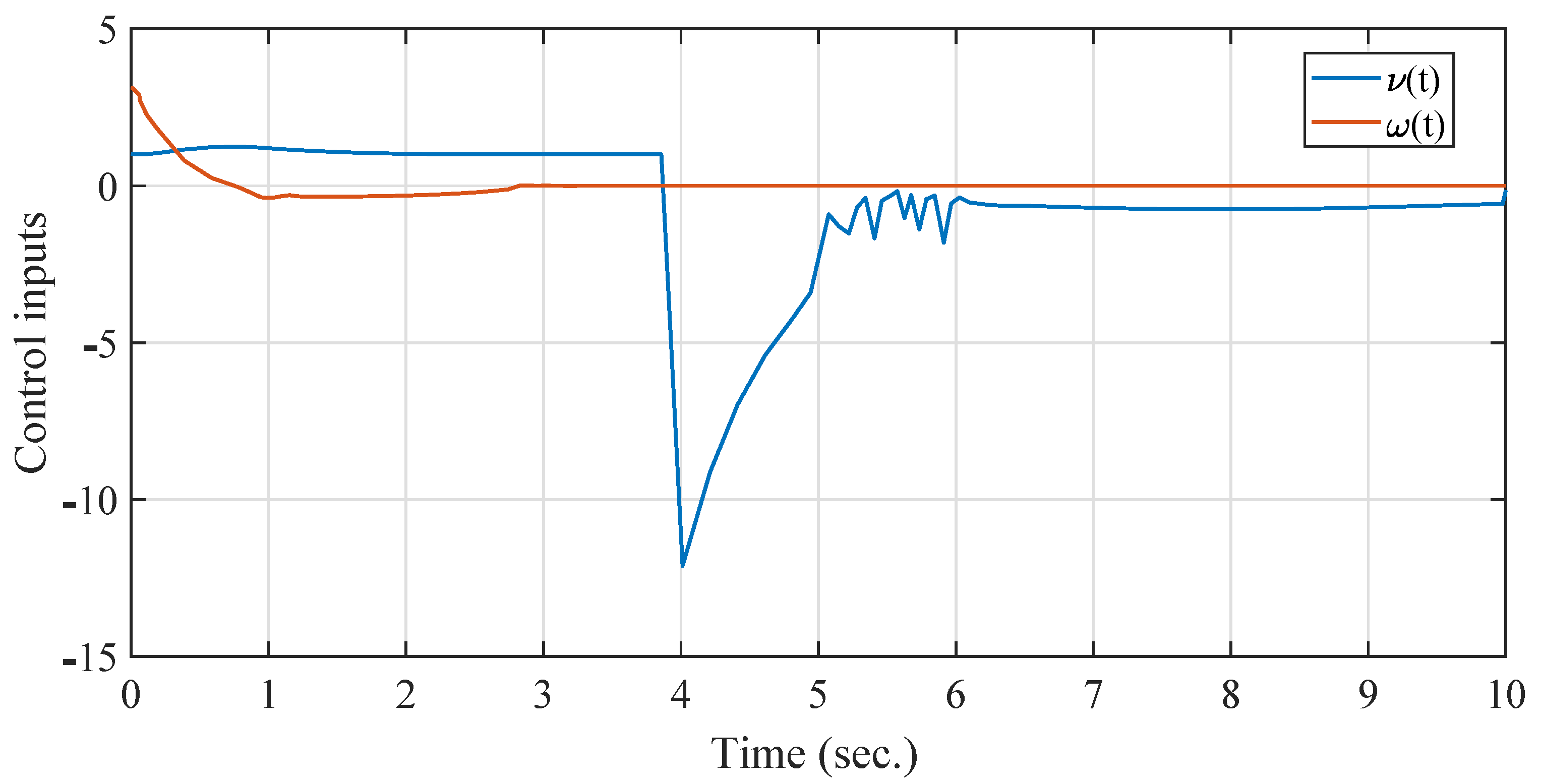
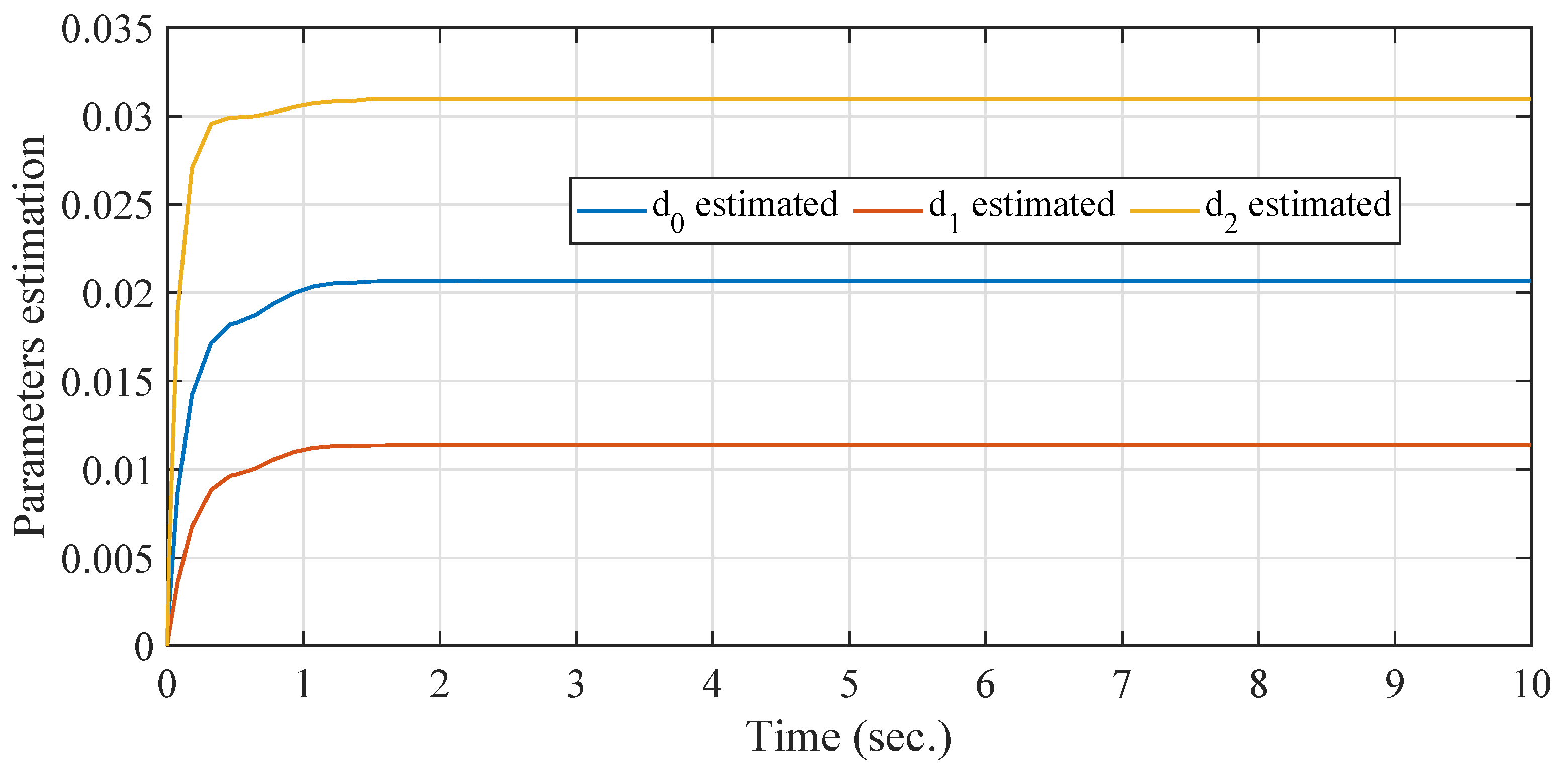
4. Analysis of the Simulation Results

In this section, the simulation studies are presented to explain the control method proposed in this paper. Consider the MR presented in Section 2 with unmatched uncertainties. Its kinematic (7) may be transformed into the system (9). When a robot functions in a constrained environment, as a result, it acts as a system stabilizer (9). The fixed-time stabilization problem of the UTMR is the main control objective. We choose the control parameters for the simulations as A 0 = 1 , α 1 = 1.2 , α 2 = 0.3 , c 0 = 0.78 , c 1 = 0.78 , c 2 = 3 , h 1 = 2 , h 2 = 0.5 , a = 0.1 , b = 1 , β 1 = 5 3 , β 2 = 2 , μ 0 = 0.0118 , μ 1 = 0.01 , and μ 2 = 0.01 . Despite the presence of perturbations, Equation (9) is a fixed-time stable system with a preset time T 1 = 4 s , thanks to the switching strategies (40) and (41).
( i ) D 0 ( t ) = 0.3 S ( 25 t ) + 0.1 C ( 10 t ) D 1 ( t ) = 0.5 S ( t ) + 0.3 C ( 15 t )
( i i ) D 0 ( t ) = 0.2 S ( t ) D 1 ( t ) = 0.3 S ( t )
and
( i i i ) D 0 ( t ) = 0.2 tanh ( 20 t 10 ) + 0.1 C ( 10 t ) D 1 ( t ) = 0.2 tanh ( 25 t 10 ) + 0.3 C ( 15 t )
The results of the proposed control scheme are presented in Figure 4, Figure 5, Figure 6, Figure 7, Figure 8, Figure 9, Figure 10, Figure 11, Figure 12 and Figure 13. As shown in Figure 4, the proposed controller’s convergence time is around 5.4 s, which is nearly constant and considerably below the predetermined duration of 10 s, as the starting value grows.
Figure 4 shows the corresponding linear and angular velocities, and Figure 5 displays the control inputs in the first case. The figures clearly show that the proposed control algorithm stabilizes the outputs of the MR under the perturbations in the fixed-time T = 4 s. The control inputs presented are smooth and have smaller magnitudes during the transients. The parameter adaptations are plotted in Figure 6, which converge to constant values. This demonstrate that all states are stable in the presence of disturbances.
The performance of the proposed controller in a 3D space is shown in Figure 7.
The state variables in the second situation are presented in Figure 8. From these results, we can see that the position and the rolling angle converge to their initial conditions under the external disturbances. From the results presented in Figure 9, we can see that the control inputs are smooth and the ANFTSMC controller is able to reject unknown disturbances. In actuality, this condition is more realistic, and the adaptive control rules are largely responsible for the stabilization of the MR. All of the parameters converge to constant values, as seen in Figure 10.
The results presented in Figure 11 represent, respectively, the state variables, the control inputs, and parameter adaptations in the last case. All state outputs are converged in the fixed-time to their initial conditions under perturbations. The inputs presented in Figure 12 are smooth and have realizable amplitudes, this demonstrates that the MR is more stable in this situation. The estimation parameters plotted in Figure 13 are converged to constant values in short finite-time.
We present the results of Defoort et al. [32] to show the superiority of our proposed approach. This technique is based on a fixed-time strategy. The same conditions are considered for our controller and the controller proposed in [32].
The controller proposed [32] in is
τ 0 = 1 i f t T 1 κ μ 1 | ε 0 | 2 s i g n ( ε 0 ) ( ς μ 1 + κ μ 2 ) s i g n ( ε 0 )
τ 1 = μ 1 + 2 ς μ 2 + 3 μ 2 ε 2 2 s i g n ( s ) s i g ( μ 3 s + μ 4 s i g ( s ) 3 ) 0.5 i f t T 1 υ i s i g n ( ε 2 ) e l s e
For which the sliding mode manifold is given by: s = ε 2 + s i g ( s i g ( ε 2 ) 2 + φ 1 ε 1 + φ 2 s i g ( ε 1 ) 3 ) 0.5 . and κ μ 1 = 0.78 , ς μ 1 = 0.78 , κ μ 2 = 0.1 , μ 1 = 4.2 , μ 2 = 4.2 , μ 3 = 2.1 , μ 4 = 2.1 , ς μ 2 = 0.3 , φ 1 = 4.2 , φ 2 = 4.2 and υ i = 0.3 .
Figure 14, Figure 15 and Figure 16 show Defoort et al.’s pertinent outcomes [32]. Their convergence time estimate is obviously greatly inflated. Additionally, it results in a bigger control magnitude during transients. The control signals have not been smooth either. It is obvious that the proposed controllers in this paper perform better than the switching control method suggested in [32].
In the second scenario, the state variables of the proposed controller are displayed in Figure 17, Figure 18 and Figure 19 [32]. These results show that the position and the rolling angle returns to its initial conditions in the presence of external perturbations. The outcomes shown in Figure 18 show that the control inputs are smooth and that the controller is capable of rejecting unidentified disturbances. This scenario is more accurate in reality, and the control methods are mostly to blame for the MR’s stability and sliding manifold’s convergence to zero.

5. Conclusions

In this paper, the stabilization problem of an NS in CFD is addressed based on fixed-time stability. A new fixed-time control approach using adaptive nonsingular fast terminal SMC is proposed for a unicycle-type mobile system with chained form dynamics under disturbances. Therefore, the adaptive-tuning control rules are used to come up with an approximation for the unknown limits of model disturbance impacting the mobile robot. Based on ANFTSMC, the robust fixed-time stabilization of the mobile robot system has been solved. A switching strategy is designed for both first- and second-order systems to guarantee the fixed-time stability. Three scenarios have shown the effectiveness of the control method proposed in this paper. According to the results, future works focus on the following points:
  • Application of this proposed control strategy in multi-agent systems;
  • Experimental validation of the proposed method.

Author Contributions

Conceptualization, M.L. and S.B.; methodology, M.L.; software, M.L.; validation, M.L., S.B. and S.K.; formal analysis, M.L.; investigation, M.L.; resources, M.L. and F.S.A.; data curation, M.L.; writing—original draft preparation, M.L., S.B. and S.K.; writing—review and editing, M.L., S.B. and S.K.; visualization, M.L., S.B. and S.K.; supervision, M.L., S.B. and S.K.; project administration, S.B. and S.K.; funding acquisition, M.L., S.B., F.S.A. and S.K. All authors have read and agreed to the published version of the manuscript.

Funding

Deputyship for Research & Innovation, Ministry of Education in Saudi Arabia—project number MoE-IF-UJ-22-04220588-1.

Data Availability Statement

The data that support the findings of this study are available from the corresponding author upon reasonable request.

Acknowledgments

The authors extend their appreciation to the Deputyship for Research & Innovation, Ministry of Education in Saudi Arabia for funding this research work through the project number MoE-IF-UJ-22-04220588-1.

Conflicts of Interest

The authors declare no conflict of interest.

References

  1. Lee, W.J.; Kwag, S.I.; Ko, Y.D. Optimal capacity and operation design of a robot logistics system for the hotel industry. Tour. Manag. 2020, 76, 103971. [Google Scholar] [CrossRef]
  2. Dutta, V.; Zielińska, T. Cybersecurity of Robotic Systems: Leading Challenges and Robotic System Design Methodology. Electronics 2021, 10, 2850. [Google Scholar] [CrossRef]
  3. Yaacoub, J.-P.A.; Noura, H.N.; Salman, O.; Chehab, A. Robotics cyber security: Vulnerabilities, attacks, countermeasures, and recommendations. Int. J. Inf. Secur. 2022, 21, 115–158. [Google Scholar] [CrossRef] [PubMed]
  4. Defoort, M.; Murakami, T. Second order sliding mode control with disturbance observer for bicycle stabilization. In Proceedings of the 2008 IEEE/RSJ International Conference on Intelligent Robots and Systems, Nice, France, 22–26 September 2008; pp. 2822–2827. [Google Scholar]
  5. Li, H.; Xie, P.; Yan, W. Receding horizon formation tracking control of constrained underactuated autonomous underwater vehicles. IEEE Trans. Ind. Electron. 2017, 64, 5004–5013. [Google Scholar] [CrossRef]
  6. Muñoz-Vázquez, J.; Parra-Vega, V.; Sánchez-Orta, A.; Sánchez-Torres, J.D. Adaptive Fuzzy Velocity Field Control for Navigation of Nonholonomic Mobile Robots. J. Intell. Robot. Syst. 2021, 101, 38. [Google Scholar] [CrossRef]
  7. Astolfi, A. Discontinuous control of nonholonomic systems. Syst. Control Lett. 1996, 27, 37–45. [Google Scholar] [CrossRef]
  8. Xu, W.L.; Huo, W. Variable structure exponential stabilization of chained systems based on the extended non-holonomic integrator. Syst. Control Lett. 2000, 41, 225–235. [Google Scholar] [CrossRef]
  9. Kolmanovsky, I.; McClamroch, N.H. Hybrid feedback laws for a class of cascade nonlinear control systems. IEEE Trans. Autom. Control 1996, 41, 1271–1282. [Google Scholar] [CrossRef]
  10. Tian, Y.P.; Li, S. Exponential stabilization of nonholonomic dynamic systems by smooth time-varying control. Automatica 2002, 38, 1139–1146. [Google Scholar] [CrossRef]
  11. Yuan, H.L.; Qu, Z.H. Smooth time-varying pure feedback control for chained nonholonomic systems with exponential convergent rate. IET Control Theory Appl. 2010, 4, 1235–1244. [Google Scholar] [CrossRef]
  12. Ge, S.S.; Wang, Z.P.; Lee, T.H. Adaptive stabilization of uncertain nonholonomic systems by state and output feedback. Automatica 2003, 39, 1451–1460. [Google Scholar] [CrossRef]
  13. Yu, J.; Zhao, Y. Global robust stabilization for nonholonomic systems with dynamic uncertainties. J. Frankl. Inst. 2019, 357, 1357–1377. [Google Scholar] [CrossRef]
  14. Gao, F.; Wu, Y.; Liu, Y. Finite-time stabilization for a class of switched stochastic nonlinear systems with dead-zone input nonlinearities. Int. J. Robust Nonlinear Control 2018, 28, 3239–3257. [Google Scholar] [CrossRef]
  15. Gao, F.; Wu, Y.; Huang, J.; Liu, Y. Output feedback stabilization within prescribed finite time of asymmetric time-varying constrained nonholonomic systems. Int. J. Robust Nonlinear Control 2021, 31, 427–446. [Google Scholar] [CrossRef]
  16. Yao, H.; Gao, F.; Huang, J.; Wu, Y. Barrier Lyapunov functions-based fixed-time stabilization of nonholonomic systems with unmatched uncertainties and time-varying output constraints. Nonl. Dyn. 2020, 99, 2835–2849. [Google Scholar] [CrossRef]
  17. Gao, F.; Huang, J.; Shi, X.; Zhu, X. Nonlinear mapping-based fixed-time stabilization of uncertain nonholonomic systems with time-varying state constraints. J. Franklin Inst. 2020, 357, 6653–6670. [Google Scholar] [CrossRef]
  18. Sánchez-Torres, J.D.; Defoort, M.; Muñoz-Vázquez, A.J. Predefined-time stabilisation of a class of nonholonomic systems. Int. J. Control 2020, 93, 2941–2948. [Google Scholar] [CrossRef]
  19. Park, B.S.; Yoo, S.J.; Park, J.B.; Choi, Y.H. Adaptive output-feedback control for trajectory tracking of electrically driven non-holonomic mobile robots. IET Control Theory Appl. 2011, 5, 830–838. [Google Scholar] [CrossRef]
  20. Muñoz-Vázquez, A.J.; Sánchez-Torres, J.D.; Parra-Vega, V.; Sánchez-Orta, A.; Martínez-Reyes, F. Robust contour tracking of nonholonomic mobile robots via adaptive velocity field motion planning scheme. Int. J. Adapt. Control Signal Process. 2019, 33, 890–899. [Google Scholar] [CrossRef]
  21. Huang, J.; Wen, C.; Wang, W.; Jiang, Z.P. Adaptive stabilization and tracking control of a nonholonomic mobile robot with input saturation and disturbance. Syst. Control Lett. 2013, 62, 234–241. [Google Scholar] [CrossRef]
  22. Polyakov, A. Nonlinear feedback design for fixed-time stabilization of linear control systems. IEEE Trans. Autom. Control 2012, 57, 2106–2110. [Google Scholar] [CrossRef]
  23. Bhat, S.; Bernstein, D. Geometric homogeneity with applications to finite time stability. Math. Control Signals Syst. 2005, 17, 101–127. [Google Scholar] [CrossRef]
  24. Yu, S.; Yu, X.; Stonier, R. Continuous finite-time control for robotic manipulators with terminal sliding modes. In Proceedings of the Sixth International Conference of Information Fusion, Cairns, Australia, 8–11 July 2003; pp. 1433–1440. [Google Scholar]
  25. Moulay, E.; Perruquetti, W. Finite time stability and stabilization of a class of continuous systems. J. Math. Anal. Appl. 2006, 323, 1430–1443. [Google Scholar] [CrossRef]
  26. Labbadi, M.; Cherkaoui, M. Robust adaptive nonsingular fast terminal sliding-mode tracking control for an uncertain quadrotor UAV subjected to disturbances. ISA Trans. 2019, 99, 290–304. [Google Scholar] [CrossRef] [PubMed]
  27. Boukattaya, M.; Mezghani, N.; Damak, T. Adaptive nonsingular fast terminal sliding-mode control for the tracking problem of uncertain dynamical systems. ISA Trans. 2018, 77, 1–19. [Google Scholar] [CrossRef] [PubMed]
  28. Lin, P.; Ma, J.; Zheng, Z. Robust adaptive sliding mode control for uncertain nonlinear MIMO system with guaranteed steady state tracking error bounds. J. Frankl. Inst. 2016, 353, 303–321. [Google Scholar]
  29. Zhihong, M.; Yu, X. Adaptive terminal sliding mode tracking control for rigid robotic manipulators with uncertain dynamics. JSME Int. J. Ser. C Mech. Syst. Mach. Elem. Manuf. 1997, 40, 493–502. [Google Scholar] [CrossRef]
  30. Yang, L.; Yang, J. Nonsingular fast terminal sliding-mode control for nonlinear dynamical systems. Int. J. Robust Nonlinear Control 2016, 21, 1865–1879. [Google Scholar] [CrossRef]
  31. Asl, S.B.F.; Moosapour, S.S. Adaptive backstepping fast terminal sliding mode controller design for ducted fan engine of thrust-vectored aircraft. Aerosp. Sci. Technol. 2017, 71, 521–529. [Google Scholar]
  32. Defoort, M.; Demesure, G.; Zuo, Z.; Polyakov, A.; Djemai, M. Fixed-time stabilisation and consensus of non-holonomic systems. IET Control Theory Appl. 2016, 10, 2497–2505. [Google Scholar] [CrossRef]
Figure 1. Indoor logistics application of mobile robots.
Mathematics 11 02287 g001
Figure 2. Last-mile mobile delivery robot (outdoors).
Mathematics 11 02287 g002
Figure 3. The planar graph of a mobile robot.
Mathematics 11 02287 g003
Figure 4. Case 1: State trajectories of the MR type unicycle in the presence of perturbations (42).
Mathematics 11 02287 g004
Figure 5. Case 1: Control inputs of the MR type unicycle.
Mathematics 11 02287 g005
Figure 6. Case 1: Parameter estimations under perturbations (42).
Mathematics 11 02287 g006
Figure 7. Case 1: Three-dimensional performance.
Mathematics 11 02287 g007
Figure 8. Case 2: State trajectories of the MR type unicycle in the presence of perturbations (43).
Mathematics 11 02287 g008
Figure 9. Case 2: Control inputs of the MR type unicycle.
Mathematics 11 02287 g009
Figure 10. Case 2: Parameter estimations under perturbations (43).
Mathematics 11 02287 g010
Figure 11. Case 3: State trajectories of the MR type unicycle in the presence of perturbations (44).
Mathematics 11 02287 g011
Figure 12. Case 3: Control inputs of the MR type unicycle.
Mathematics 11 02287 g012
Figure 13. Case 3: Parameter estimations under perturbations (44).
Mathematics 11 02287 g013
Figure 14. Case 1: State trajectory graphs correspond to the controller in [32].
Mathematics 11 02287 g014
Figure 15. Case 1: Control inputs obtained by the controller in [32].
Mathematics 11 02287 g015
Figure 16. Case 1: Evolution of the sliding manifold using the controller in [32].
Mathematics 11 02287 g016
Figure 17. Case 2: State trajectory graphs that correspond to the controller in [32].
Mathematics 11 02287 g017
Figure 18. Case 2: Control inputs obtained by the controller in [32].
Mathematics 11 02287 g018
Figure 19. Case 2: Evolution of the sliding manifold using the controller in [32].
Mathematics 11 02287 g019
Disclaimer/Publisher’s Note: The statements, opinions and data contained in all publications are solely those of the individual author(s) and contributor(s) and not of MDPI and/or the editor(s). MDPI and/or the editor(s) disclaim responsibility for any injury to people or property resulting from any ideas, methods, instructions or products referred to in the content.

