Adjacent Vertex Distinguishing Coloring of Fuzzy Graphs

Abstract

In this paper, we consider the adjacent vertex distinguishing proper edge coloring (for short, AVDPEC) and the adjacent vertex distinguishing total coloring (for short, AVDTC) of a fuzzy graph. Firstly, this paper describes the development process, the application areas, and the existing review research of fuzzy graphs and adjacent vertex distinguishing coloring of crisp graphs. Secondly, we briefly introduce the coloring theory of crisp graphs and the related theoretical basis of fuzzy graphs, and add some new classes of fuzzy graphs. Then, based on the $\alpha$-cuts of fuzzy graphs and distance functions, we give two definitions of the AVDPEC of fuzzy graphs, respectively. A lower bound on the chromatic number of the AVDPEC of a fuzzy graph is obtained. With examples, we show that some results of the AVDPEC of a crisp graph do not carry over to our set up; the adjacent vertex distinguishing chromatic number of the fuzzy graph is different from the general chromatic number of a fuzzy graph. We also give a simple algorithm to construct a $(d,f)$-extended AVDPEC for fuzzy graphs. After that, in a similar way, two definitions of the AVDTC of fuzzy graphs are discussed. Finally, the future research directions of distinguishing coloring of fuzzy graphs are given.

1. Introduction

As is known to all, graph coloring has always been one of the important problems in graph theory research, and it has important theoretical and practical significance. In our real life, the solution of many practical problems can often be summed up as graph coloring. For example, the points could represent people, with lines joining pairs of friends; or the points might be communication centres, with lines representing communication links; or vertices could represent animals, with lines joining animals with the same properties. Notice that in such diagrams, one is mainly interested in whether two given points are joined by a line; the manner in which they are joined is immaterial. The mathematical abstraction of this situation gave rise to the concept of graphs in classical graph theory. In classical graph theory, the edge of a graph can only indicate whether there is a binary relation, but not the degree of the relation.

Fuzzy-set theory, introduced by Zadeh [1], is a mathematical tool to handle uncertainties, such as vagueness, ambiguity, and imprecision in linguistic variables. The combination of fuzzy theory and graph theory produces fuzzy graphs that solve the problem of describing the degree of relationship. The first definition of fuzzy graph was proposed by Kaufmann [2], from the fuzzy relations introduced by Zadeh. Rosenfeld [3] introduced another elaborated definition, including fuzzy vertices and fuzzy edges. The fuzzy graph solves the problem of describing the relation degree between objects. Subsequently, many scholars have made many generalizations of fuzzy graphs. For instance, Mordeson et al. [4] introduced the operations of Cartesian product, composition, union, and join on fuzzy graphs. The work in [5] investigated the isomorphic properties of direct product, a strong product of complete fuzzy graphs. Mohinta et al. [6] proposed the concepts of fuzzy soft graph, and union and intersection of two fuzzy soft graphs based on soft set theory [7,8], and established some properties related to finite union and intersection of fuzzy soft graphs. Masarwah [9] presented some new concepts of fuzzy soft graphs with the notions of complement and $\mu$-complement fuzzy soft graphs, and also obtained a few properties related to the complement of strong fuzzy soft graphs and complete fuzzy soft graphs. Gong and Wang [10] discussed the operations of fuzzy hypergraphs and strong fuzzy r-uniform hypergraphs, such as Cartesian product, strong product, normal product, lexicographic product, union, and join. Since then, they have proposed a hesitant fuzzy hypergraph model and studied some operations and equivalence relations for hesitant fuzzy hypergraphs in [11]. Recently, Sreenanda et al. [12] investigated a comprehensive study on perpect fuzzy graphs, including the relationship between the chromatic numbers of a fuzzy graph and its complement graph, and the relationship between the perfection of a fuzzy graph and its underlying crisp graph. The readers may refer to [13,14,15] for more detail in the research on fuzzy graphs.

Given that the coloring of fuzzy graphs plays an irreplaceable role in practical problems such as task assignment and conflict coordination, more and more scholars are devoted to the study of fuzzy graph coloring problems. Proper coloring of a crisp graph requires that the same color not be used between adjacent vertices, adjacent edges, and associated vertices and edges. An important objective of coloring is to minimize the number of colors while coloring a graph. Many coloring definitions from classical graph theory have been generalized to fuzzy graphs or fuzzy hypergraphs, such as vertex coloring [16], edge coloring [17], fractional coloring [18], etc. However, there are still many coloring problems in classical graph theory that have not yet found corresponding definitions in fuzzy graphs, such as adjacent vertex distinguishing coloring, circle coloring, relax coloring, etc. Our work will fill this gap. In this paper, we will extend the adjacent vertex distinguishing proper edge coloring and the adjacent vertex distinguishing total coloring to the fuzzy graph in two ways. The following is a review of the two adjacent vertex distinguishing coloring problems in the crisp graph.

The concept that the adjacent vertex distinguishes proper edge coloring (for short, AVDPEC) was introduced by Zhang et al. [19] in 2002; they proposed the AVDPEC conjecture based on the discussion of the adjacent vertex distinguishing proper edge chromatic numbers of trees, circles, complete bipartite graphs, and complete graphs. The research on the adjacent vertex distinguishing proper edge coloring mainly focuses on AVDPEC conjecture.

For regular graphs, there is a close relationship between the adjacent vertex distinguishing proper edge coloring and the proper total coloring. Therefore, with the help of the proper total coloring, it is easy to obtain the adjacent vertex distinguishing proper edge chromatic number of balanced complete multipartite graphs and $k$-cubes. This idea was proposed by Zhang et al. in reference [20]. Vizing [21] and Behzad [22] independently gave the Total Coloring conjecture (TC conjecture). Once a k-regular graph satisfies both AVDPEC conjecture and TC conjecture, then the adjacent vertex distinguishing proper edge chromatic number of the graph is equal to the total chromatic number.

In 2004, on the basis of total coloring of the crisp graphs, Zhang et al. [23] proposed a new concept of distinguishable total staining of adjacent points of graphs, which generated a new interesting topic in the theory of graph coloring, and some valuable results have been obtained. They discussed the adjacent vertex distinguishing (proper) total colouring (for short, AVDTC) of the graphs obtained by deleting an edge of circle, complete graph, complete bipartite graph, fan, wheel, tree and odd-order complete graph, and determined the adjacent vertex distinguishing (proper) total chromatic number of these graphs. At the same time, based on these results, a conjecture $({\chi }_{at}^{\prime }(G)\le \Delta (G)+3$ for a simple connected graph G of order no less than 2, ${\chi }_{at}^{\prime }(G)$ in this formula is the adjacent vertex distinguishing total chromatic number of graph G) is proposed. In reference [24], the adjacent distinguishing coloring number of direct product graph $P_m\times K_n$ of m-order path $P_m$ and n-order complete graph $K_n$ is given. The results of adjacent distinguishing total coloring are more extensive and can be found in [25,26,27].

In 1955, Mycielski [28] constructed a new graph $\mathcal{M}(G)$ from a graph G, now called $\mathcal{M}(G)$ as the Mycielski graph of G, which solved the problem of the existence of non-triangular graphs with large chromatic number but small clique number. The structure of this graph has aroused great interest in many scholars and a series of good results have been obtained. Various staining of the Mycielski graph of a graph is valued. In this paper, besides giving the definitions of fuzzy star, fuzzy fan, and fuzzy wheel, the Mycielski graph is also promoted, and the Mycielski graph of fuzzy graph $\tilde{G}$ and k-multi-Mycielski graphs of fuzzy graph $\tilde{G}$ are obtained.

Following the reference [16], this paper extends the adjacent vertex distinguishing total coloring crisp graphs to fuzzy graphs with crisp vertex set and fuzzy edge set. The AVDPEC and AVDTC of a fuzzy graph are defined by two different approaches. The first approach is based on the successive coloring AVDPEC function ${\phi }_{\alpha }$ (or AVDTC function ${\psi }_{\alpha }$) of the crisp graphs $G_{\alpha }=(V,E_{\alpha })$ represented the $\alpha$-cuts of $\tilde{G}$. The second approach is based on an extension of the concept of AVDPEC-function (or AVDTC-function) by means of a distance defined between colors; an extended coloring function is introduced based on the adjacent vertex distinguishing proper edge coloring of the support graph of a fuzzy graph. Section 3 and Section 4 will discuss the adjacent vertex distinguishing proper edge coloring and the adjacent vertex distinguishing total coloring of fuzzy graphs based on the above two approaches, respectively.

In addition, there is an interesting property of adjacent distinguished total coloring: the adjacent vertex distinguishing total chromatic number of subgraphs is not necessarily smaller than that of parent graphs. For example, G is a 4-order graph obtained by bonding a vertex between the complete graph $K_3$ and $K_2$, where $4={\chi }_{at}(G)<{\chi }_{at}(K_3)=5$. Therefore, Zhang et al. [20] proposed an open question (if H is a subgraph of G, under what circumstances can there be ${\chi }_{at}(H)\le {\chi }_{at}(G)$?). Similarly, the adjacent distinguishing proper edge coloring problem proposed by Zhang et al. [19] has the same characteristics (for example, the adjacent vertex distinguishing proper edge chromatic number of 5-circle $C_5=v_1{v}_2{v}_3{v}_4{v}_5{v}_1$ is equal to 5, add an edge $v_1{v}_3$ to $C_5$, in the newly obtained graph, the number of adjacent distinguishing edge colors is reduced to 4), which fully demonstrates the difficulty of the adjacent distinguishing total coloring and adjacent distinguishing proper edge coloring.

The above interesting property, when extended to a fuzzy graphs, is manifested by the loss of sequence monotonicity, which is different from the coloring of fuzzy graphs defined in [16]. This can be shown by Example 6 and Example 8.

2. Preliminaries

In this section, we first recall some definitions and lemmas in graph theory, fuzzy set theory, and fuzzy graph coloring that will be used in constructing chromatic number of fuzzy graphs. Then, the definitions of some fuzzy graphs are introduced.

2.1. Three Kinds of Coloring of a Crisp Graph

The basic definitions used here are adopted from [28] with little modifications.

A graph G is an ordered pair$(V,E)$ consisting of a set V of vertices and a set E, disjointed from V of edges, together with an incidence function $f_G$ that associates with each edge of G an unordered pair of (not necessarily distinct) vertices of G. If e is an edge and u and v are vertices such that $f_G(e)=uv$ or $f_G(e)=vu$, then e is said to join u and v, and the vertices u and v are called the ends of e. We denote the numbers of vertices and edges in G by $\left|V\right|$ and $\left|E\right|$; these two basic parameters are called the order and size of G, respectively.

An edge with identical ends is called a loop, and two or more links with a pair of ends are said to be parallel edges. The ends of an edge are said to be incident with the edge, and vice versa. Two vertices which are incident with a common edge are adjacent, as are two edges which are incident with a common vertex, and two distinct adjacent vertices are neighbors. For an edge e of a graph G, we call e an isolated edge if it has no neighbors in G. One example of graphs should serve to clarify the above definition.

Example 1. 

(i) Let $G=(V_1,E_1)$ be a crisp graph, where $V_1=\{v_1,v_2,v_3,v_4\}$, $E_1=\{e_1,e_2,e_3,e_4,e_5,e_6,e_7\}$, and $f_G$ is defined by

$$f_G(e_1)=v_1{v}_1,f_G(e_2)=v_1{v}_2,f_G(e_3)=v_2{v}_3,$$

$$f_G(e_4)=v_2{v}_3,f_G(e_5)=v_3{v}_4,f_G(e_6)=v_4{v}_1,f_G(e_7)=v_2{v}_4.$$

(ii) Let $H=(V_2,E_2)$ be a crisp graph, where $V_2=\{u_1,u_2,u_3,u_4\}$, $E_2=\{a,b,c,d,e\}$, and $f_H$ is defined by

$$f_H(l_1)=u_1{u}_2,f_H(l_2)=u_2{u}_3,f_H(l_3)=u_3{u}_4,$$

$$f_H(l_4)=u_4{u}_1,f_H(l_5)=u_2{u}_4,f_H(l_6)=u_5{u}_6.$$

Diagrams of G and H are shown in Figure 1.

In the graph G of Figure 1, the edge $e_1$ is a loop, and the edges $e_3$ and $e_4$ are parallel edges. $l_6$ is an isolated edge because it has no neighbors in H. A graph is simple if it has no loops or parallel edges. The graph H in Example 1(ii) is simple, whereas the graph G in Example 1(i) is not. If we remove the rings in G and keep only one of the parallel edges, we have a simple graph of G.

The graphs involved in this paper are all undirected graphs without rings and parallel edges.

For a crisp graph G, if $\varphi$ is a mapping from $V(G)\cup E(G)$ to $\{1,2,\dots ,k\}$ such that (i) $\varphi (v_i{v}_j)\ne \varphi (v_i{v}_k),\varphi (v_i{v}_j)\ne \varphi (v_l{v}_j)$, for all edge $v_i{v}_j,v_i{v}_k,v_l{v}_j\in E$, (ii) $\varphi (v_i)\ne \varphi (v_j)$, if edge $v_i{v}_j\in E$, then $\phi$ is said to be a total coloring of G. A k-total coloring is a total coloring using at most k colors. Let ${\chi }_t(G)$ be the minimum number of colors in a total-coloring of G. $\Delta (G)$ is the maximum degree of any vertex in G. The edge coloring satisfying condition (i) is called a proper edge coloring, while the vertex coloring satisfying condition (ii) is called a proper vertex coloring. All the coloring mentioned in this paper is proper coloring.

We say a proper edge coloring of G is an adjacent vertex distinguishing proper edge coloring (for short, AVDPEC), if for any pair of adjacent vertices u and v, the set of colors incident to u is not equal to the set of colors incident to v. It is clear that an AVDPEC exists provided G contains no isolated edge. In other words, given a graph $G=(V,E)$, an AVDPEC is a function $\phi :E\to \{1,2,\dots ,k\}$ such that (i) $\phi (v_i{v}_j)\ne \phi (v_i{v}_k),\phi (v_i{v}_j)\ne \phi (v_l{v}_j)$, for all edge $v_i{v}_j,v_i{v}_k,v_l{v}_j\in E$, (ii) the set of colors incident to u denoted by $S_{\phi }(u)$, $S_{\phi }(u)\ne S_{\phi }(v)$ for any pair of adjacent vertices u and v. A k-AVDPEC is an AVDPEC using at most k colors. Let ${\chi }_a^{\prime }(G)$ be the minimum number of colors in an AVDPEC of G.

The adjacent vertex distinguishing total coloring (for short, AVDTC) of G refers to any pair of adjacent vertices u and v; the set of colors incident to u is not equal to the set of colors incident to v. In other words, given a graph $G=(V,E)$, an AVDTC is a function $\psi :V\cup E\to \{1,2,\dots ,k\}$ such that (i) $\psi (v_i{v}_j)\ne \psi (v_i{v}_k),\psi (v_i{v}_j)\ne \psi (v_l{v}_j)$, for all edge $v_i{v}_j,v_i{v}_k,v_l{v}_j\in E$, (ii) $\psi (v_i)\ne \psi (v_j)$, if edge $v_i{v}_j\in E$, (iii) the set of colors incident to u denoted by $S_{\psi }(u)$, $S_{\psi }(u)\ne S_{\psi }(v)$ for any pair of adjacent vertex u and v. A k-AVDTC is an AVDTC using at most k colors. Let ${\chi }_{at}(G)$ be the minimum number of colors in an AVDTC of G.

In the problem of adjacent distinguishable coloring of graphs, it is required that there are no loops, parallel edges, or isolated edges in the graph. This is because the color set of vertices associated with isolated edges and rings must be indistinguishable. The adjacent vertex distinguishing the coloring problem of a graph with multiple edges can be converted to the adjacent vertex distinguishing coloring of its corresponding simple graph.

Lemma 1 

([23]). For the graph G without isolated edges, ${\chi }_a^{\prime }(G)\ge \Delta (G)$.

Lemma 2 

([23]). Let G be a simple connected graph of order not less than 2, then (i) ${\chi }_{at}(G)\ge \Delta (G)+1$, (ii) when two maxima degree vertices in G are adjacent, ${\chi }_{at}(G)\ge \Delta (G)+2$.

From [19], we know some basic facts such as that there must exist an adjacent vertex distinguishing proper edge coloring of connected graphs without isolated edges or an order of at least 3. There are also many examples of graphs for which ${\chi }_a^{\prime }(G)>\Delta (G)+1$, see [19,20,29,30,31,32]. Akbari et al., in reference [33], gave an upper bound on the color number of the adjacent vertex distinguishing proper edge coloring (if graph G contains no isolated edges, then ${\chi }_a^{\prime }(G)\le 3\Delta (G)$). Hatami [34] has recently shown using probabilistic methods that ${\chi }_a^{\prime }(G)\le \Delta (G)+300$ for sufficiently large $\Delta (G)$. In other cases, the upper bound of the chromatic number of graph G can be found in reference [30].

In addition to the upper and lower results for the two adjacent vertices distinguishing chromatic numbers, the corresponding adjacent vertices distinguishing chromatic numbers for a large number of specific crisp graphs are also obtained in [19,20,23,24,31,32,35]. Lemmas 3–8 list some possible results that may be used in this paper.

Lemma 3 

([19]). For a complete graph $K_n$ with $|V(K_n)|\ge 3$, then

$${\chi }_a^{\prime }(K_n)=\left\{\begin{array}{cc}\hfill n+1,& n\equiv 0(\mathit{mod}2),\hfill \\ \hfill n,& n\equiv 1(\mathit{mod}2).\hfill \end{array}\right.$$

Lemma 4 

([19]). For a circle $C_n$ with $|V(C_n)|\ge 3$, then

$${\chi }_a^{\prime }(C_n)=\left\{\begin{array}{cc}\hfill 3,& n\equiv 0(\mathit{mod}3),\hfill \\ \hfill 4,& n\not\equiv 0(\mathit{mod}3),n\ne 5,\hfill \\ \hfill 5,& n=5.\hfill \end{array}\right.$$

Lemma 5 

([19]). For a tree $T_n$ with $|V(T_n)|\ge 3$, (1) if any two vertices of maximum degree are not adjacent, then ${\chi }_a^{\prime }(T_n)=\Delta (T_n)$; (2) if T has two vertices of maximum degree which are adjacent, then ${\chi }_a^{\prime }(T_n)=\Delta (T_n)+1$.

Lemma 6 

([23]). For a compete graph $K_n$ with $|V(K_n)|\ge 3$, then

$${\chi }_{at}(K_n)=\left\{\begin{array}{cc}\hfill n+1,& n\equiv 0(\mathit{mod}2),\hfill \\ \hfill n+2,& n\equiv 1(\mathit{mod}2).\hfill \end{array}\right.$$

Lemma 7 

([23]). For a tree $T_n$ with $|V(T_n)|\ge 3$, (1) if any two vertices of maximum degree are not adjacent, then ${\chi }_{at}(T_n)=\Delta (T_n)+1$; (2) if T has two vertices of maximum degree which are adjacent, then ${\chi }_{at}(T_n)=\Delta (T_n)+2$.

Lemma 8 

([23]). For a circle $C_n$ with $|V(C_n)|\ge 3$, then

$${\chi }_{at}^{\prime }(C_n)=\left\{\begin{array}{cc}\hfill 4,& n\ge 4,\hfill \\ \hfill 5,& n=3.\hfill \end{array}\right.$$

Other terminology and symbols related to the coloring theory of graphs used in this paper can be found in [20].

2.2. Basic Concepts in Fuzzy Sets

We will use the classical definition of fuzzy set A defined on a empty set X as the family $A=\{(x,{\mu }_A(x))\mid x\in X\}$ where ${\mu }_A:X\to [0,1]$ is the membership function and ${\mu }_A(x)$ denotes the degree to which x belongs to A. ${\mu }_A(x)=0$ indicates that x does not belong to A, and any intermediate value represents the degree to which x could belong to A. We denote by $\tilde{F}(X)$ the collection of all fuzzy subsets of X.

Fuzzy sets are generalizations of the classical sets represented by their characteristic functions ${\mu }_{\tilde{A}}:X\to [0,1]$. In our case, $\tilde{A}=1$ means full membership of x in $\tilde{A}$, while $\tilde{A}=0$ express nonmembership, but in contrary to the classical set, other membership degrees are allowed.

Definition 1 

([36]). Let $\tilde{A}:X\to [0,1]$ be a fuzzy set. The level sets of $\tilde{A}$ are defined as the classical sets

$$A_{\alpha }=\{x\in X\mid \tilde{A}\ge \alpha \},0<\alpha \le 1.$$

$$A_1=\{x\in X\mid \tilde{A}=1\}$$

is called the core of the fuzzy set $\tilde{A}$, and 

$$\mathrm{supp}\tilde{A}=\{x\in X\mid \tilde{A}>0\}$$

is called the support of the fuzzy set.

Definition 2 

([36]). Let $\tilde{A},\tilde{B}\in \tilde{F}(X)$. We say that the fuzzy set $\tilde{A}$ is included in $\tilde{B}$ if

$$\tilde{A}(x)\le \tilde{B}(x),\mathit{for}\mathit{all}x,y\in X.$$

We denote $\tilde{A}\subseteq \tilde{B}$.

Definition 3 

([36]). Let σ be a fuzzy subset of a set S and μ be a fuzzy relation on S. The μ is called a fuzzy relation on σ if

$$\mu (x,y)\le \sigma (x)\wedge \sigma (y),\mathit{for}\mathit{all}x,y\in S.$$

A fuzzy relation μ is symmetric if $\mu (x,y)=\mu (y,x)\mathit{for}\mathit{all}x,y\in X$.

Definition 4 

([3]). Let $\tilde{G}(\tilde{V},\tilde{E})$ be a fuzzy graph, where the fuzzy vertex set $\tilde{V}$ is a non-empty set V together with a pair of function $\rho :V\to [0,1]$ and the fuzzy edge set $\tilde{E}$ is characterised by the matrix $\mu ={({\mu }_{ij})}_{v_i,v_j\in V}$:

$${\mu }_{ij}={\mu }_{\tilde{E}}(v_i{v}_j),\forall v_i,v_j\in V,$$

such that $i\ne j$, ${\mu }_{ij}\le \min \{\rho (v_i),\rho (v_j)\}$ and ${\mu }_{\tilde{E}}:V\times V\to [0,1]$ is the membership function.

In this paper, we consider a fuzzy graph in which $\rho (v)=1$ for any $v\in V$. Hence, a fuzzy graph can be denoted by $\tilde{G}(V,\tilde{E})$ or $\tilde{G}(V,\mu )$. The fuzzy graph $\tilde{G}$ becomes a crisp graph if matrix $\mu$ defined as

$${\mu }_{ij}=\left\{\begin{array}{cc}\hfill 1,& \mathrm{if}{v}_i{v}_j\in \tilde{E},\hfill \\ \hfill 0,& \mathrm{otherwise},\hfill \end{array}\right.$$

for all $v_i,v_j\in V.$

In order to define more precisely the adjacent vertex distinguishing coloring of the fuzzy graphs, we need to extend the concepts of adjacent vertices, adjacent edges, degrees of vertices, and isolated edges in the crisp graphs to the fuzzy graphs.

Definition 5. 

(Adjacent vertices in fuzzy graph) Let $\tilde{G}(V,\tilde{E})$ be a fuzzy graph, μ be the membership function of $\tilde{E}$. For a given vertex u in vertex set V, the vertex v is said to be the adjacent fuzzy vertex when ${\mu }_{\tilde{E}}(uv)>0$, for all $v\in V$.

Definition 6. 

(Adjacent fuzzy edge) Let $\tilde{G}(V,\tilde{E})$ be a fuzzy graph, μ be the membership function of $\tilde{E}$. For a given fuzzy edge $v_i{v}_j({\mu }_{ij}>0)$ in fuzzy edge set $\tilde{E}$, the fuzzy edge $\{v_i{v}_l\mid {\mu }_{il}>0\}$ and $\{v_k{v}_j\mid {\mu }_{kj}>0\}$ are called the adjacent fuzzy edge of fuzzy edge $v_i{v}_j$.

Definition 7. 

(The degree of a vertex in a fuzzy graph) Let $\tilde{G}(V,\tilde{E})$ be a fuzzy graph and μ be the membership function of $\tilde{E}$. The degree of a vertex u in the graph $\tilde{G}$ is the number of elements in the fuzzy edges set $\{uv\mid \forall v\in V,{\mu }_{\tilde{E}}(uv)>0\}$, denoted by $d_{\tilde{G}}(u)$.

Remark 1. 

Let $\tilde{G}=(V,\tilde{E})$ be a fuzzy graph, and if we call the crisp graph graph $G=(V,\mathrm{supp}\tilde{E})$ a support graph of $\tilde{G}=(V,\tilde{E})$, then many concepts on classical graph theory can be automatically applied to fuzzy graphs. For example, if we call $\tilde{G}$ a simple graph, it means that its support graph is a simple graph, i.e., a graph without multiple edges and rings; similarly, if $\tilde{G}$ is an empty graph, it means that $\tilde{G}$ has neither vertices nor fuzzy edges; if $\tilde{G}$ does not contain isolated edges, it means that its support graph G does not contain isolated edges, etc. The terminology of classical graph theory can be transferred to fuzzy graphs without the definite term “Fuzzy” in the name.

Alternatively, the isolated edges contained in the fuzzy graph $\tilde{G}$ can also be inscribed by the degree of the vertices in the fuzzy graph given in Definition 8.

Definition 8. 

(The isolated edge of a fuzzy graph) Let $\tilde{G}=(V,\tilde{E})$ be a fuzzy graph. A fuzzy edge $uv$ is called an isolated edge of a fuzzy graph $\tilde{G}$ if $uv\in \tilde{E}$ and $d_{\tilde{G}}(u)=d_{\tilde{G}}(v)=1$.

Definition 9 

([37]). Let $\tilde{G}(V,\tilde{E})$ and ${\tilde{G}}_1(V_1,{\tilde{E}}_1)$ be two fuzzy graphs; the fuzzy graph ${\tilde{G}}_1(V_1,{\tilde{E}}_1)$ is called fuzzy subgraph of $\tilde{G}$, if $V_1\subseteq V$ and ${\tilde{E}}_1\subseteq \tilde{E}$, denoted by ${\tilde{G}}_1(V_1,{\tilde{E}}_1)\subseteq \tilde{G}(V,\tilde{E})$.

Definition 10 

([37]). Let ${\tilde{G}}_1(V_1,{\tilde{E}}_1)$ and ${\tilde{G}}_2(V_2,{\tilde{E}}_2)$ be two fuzzy graphs; ${\mu }_1$ and ${\mu }_2$ be the membership functions of ${\tilde{E}}_1$ and ${\tilde{E}}_2$, respectively. We will say that ${\tilde{G}}_1$ and ${\tilde{G}}_2$ are isomorphic, denoted by ${\tilde{G}}_1\cong {\tilde{G}}_2$, if there exists a bijection $h:V_1\to V_1$ such that ${\mu }_1(uv)={\mu }_2(h(u)h(v))$ for any $u,v\in V_1$.

Theorem 1. 

Let ${\tilde{G}}^1(V_1,{\tilde{E}}_1)$ and ${\tilde{G}}^2(V_2,{\tilde{E}}_2)$ be two fuzzy graphs where the membership functions of ${\tilde{E}}_1$ and ${\tilde{E}}_2$ are ${\mu }_1$ and ${\mu }_2$, respectively. ${\tilde{G}}_{\alpha }^1$ and ${\tilde{G}}_{\alpha }^2$ ($\alpha \in [0,1]$) be the $\alpha$-cut of ${\tilde{G}}^1$ and ${\tilde{G}}^2$, respectively. If ${\tilde{G}}^1\cong {\tilde{G}}^2$, then ${\tilde{G}}_{\alpha }^1\cong {\tilde{G}}_{\alpha }^2$.

Proof. 

Since ${\tilde{G}}^1\cong {\tilde{G}}^2$, there exists a bijection $h:V_1\to V_2$ such that ${\mu }_1(u,v)={\mu }_2(h(u),h(v))$ for any $u,v\in V_1$. Because of $V_1=V({\tilde{G}}_{\alpha }^1)$ and $V_2=V({\tilde{G}}_{\alpha }^2)$, there exists a bijection $h^{*}:V({\tilde{G}}_{\alpha }^1)\to V({\tilde{G}}_{\alpha }^2)$ such that ${\mu }_1(uv)={\mu }_2(h^{*}(u)h^{*}(v))$ for any $u,v\in V({\tilde{G}}_{\alpha }^1)$, i.e., ${\tilde{G}}_{\alpha }^1\cong {\tilde{G}}_{\alpha }^2$, $\alpha \in [0,1]$.    □

2.3. Some Particular Fuzzy Graph

The concepts of fuzzy graphs such as fuzzy trees, fuzzy forests, and fuzzy circles were introduced in [38], and some new fuzzy graphs are added in this part.

Definition 11. 

(Mycielski graph of fuzzy graph $\tilde{G}$) Let $\tilde{G}(V,\tilde{E})$ be a fuzzy graph, μ be the membership function of $\tilde{E}$. $\mathcal{M}(\tilde{G})$ is called a Mycielski graph if $V(\mathcal{M}(\tilde{G}))=\{v_0,v_1,\dots ,v_{n-1}\}\cup \left\{u\right\}$, $\tilde{E}(\mathcal{M}(G))=\tilde{E}(\tilde{G})\cup \{v_{j}u\mid j=0,1,\dots ,n-1,{\mu }_{\tilde{E}}(v_{j}u)>0\}$.

Definition 12. 

(k-multi-Mycielski graphs of fuzzy graph $\tilde{G}$) Let $\tilde{G}(V,\tilde{E})$ be a fuzzy graph, μ be the membership function of $\tilde{E}$. ${\mathcal{M}}^k(\tilde{G})$ is called a k-multi-Mycielski graph, if  (1) $V({\mathcal{M}}^k(\tilde{G}))=\{v_{00},v_{01},\dots ,v_{0,n-1};v_{10},v_{11},\dots ,v_{1,n-1};\dots ;v_{k0},v_{k1},\dots ,v_{k,n-1}\}\cup \left\{u\right\}$,

(2) $\tilde{E}({\mathcal{M}}^k(\tilde{G}))=\tilde{E}(\tilde{G})\cup \{v_{ij}{v}_{i+1,l}\mid v_{0j}{v}_{0l}\in \tilde{E}(\tilde{G}),{\mu }_{\tilde{E}({\mathcal{M}}^k(\tilde{G}))}(v_{ij}{v}_{i+1,l})={\mu }_{\tilde{E}(G)}(v_{0j}{v}_{0l}),0\le i,k\le n-1,i=0,1,\dots ,k-1\}\cup \{v_{kj}u\mid j=0,1,\dots ,n-1,{\mu }_{\tilde{E}({\mathcal{M}}^k(\tilde{G}))}(v_{kj}u)>0\}$.

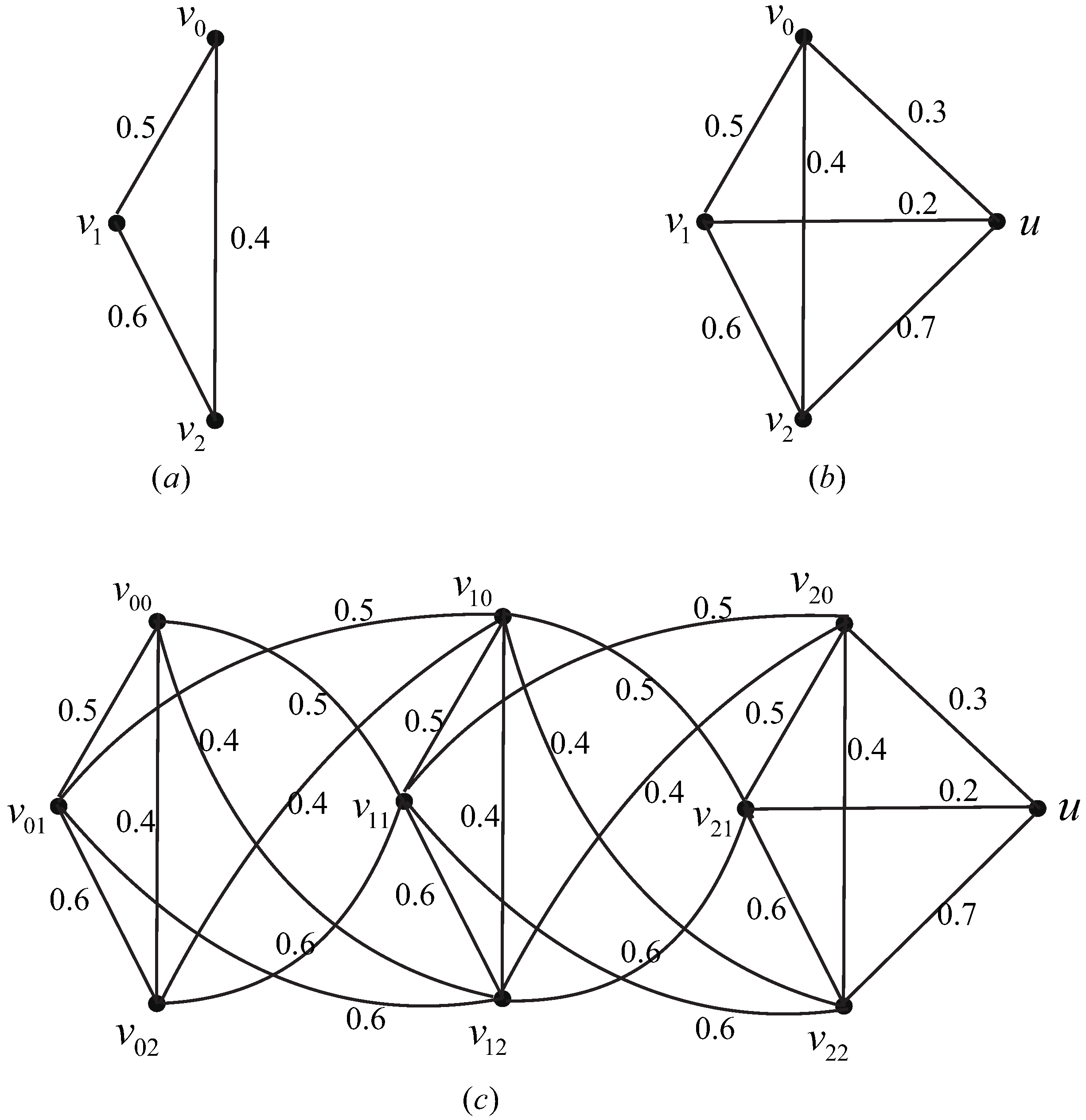
Example 2. 

Given a fuzzy graph $\tilde{G}=(V,\tilde{E})$, where $V=\{v_1,v_2,v_3\}$,  the membership function of $\tilde{E}$ is μ as follows.

$$\mu =\left[\begin{array}{ccc}-& 0.5& 0.4\\ 0.5& -& 0.6\\ 0.4& 0.6& -\end{array}\right].$$

By Definitions 11 and 12, we can obtain a Mycielski graph of fuzzy graph $\mathcal{M}(\tilde{G})(V_1,{\tilde{E}}_1)$ and a 2-multi-Mycielski graph of fuzzy graph ${\mathcal{M}}^k(\tilde{G})(V_2,{\tilde{E}}_2)$, where $V_1=\{v_1,v_2,v_3,u\}$, $V_2=\{v_{00},v_{01},v_{02};v_{10},v_{11},v_{12};v_{20},v_{21},\dots ,v_{22};u\}$; the membership functions of ${\tilde{E}}_1$ and ${\tilde{E}}_2$ are ${\mu }_1$ and ${\mu }_2$, respectively.

$${\mu }_1=\left[\begin{array}{cccc}-& 0.5& 0.4& 0.3\\ 0.5& -& 0.6& 0.2\\ 0.4& 0.6& -& 0.7\\ 0.3& 0.2& 0.7& -\end{array}\right],$$

$${\mu }_2=\left[\begin{array}{cccccccccc}-& 0.5& 0.4& -& 0.5& 0.4& -& -& -& -\\ 0.5& -& 0.6& 0.5& -& 0.6& -& -& -& -\\ 0.4& 0.6& -& 0.4& 0.6& -& -& -& -& -\\ -& 0.5& 0.4& -& 0.5& 0.4& -& 0.5& 0.4& -\\ 0.5& -& 0.6& 0.5& -& 0.6& 0.5& -& 0.6& -\\ 0.4& 0.6& -& 0.4& 0.6& -& 0.4& 0.6& -& -\\ -& -& -& -& 0.5& 0.4& -& 0.5& 0.4& -\\ -& -& -& 0.5& -& 0.6& 0.5& -& 0.6& 0.3\\ -& -& -& 0.4& 0.6& -& 0.4& 0.6& -& 0.2\\ -& -& -& -& -& -& -& 0.3& 0.2& 0.7\end{array}\right].$$

For simplicity, we show only the computing of ${\mu }_2(v_{0j}{v}_{1l})$. By Definition 12, we have

$${\mu }_2(v_{00}{v}_{11})={\mu }_2(v_{00}{v}_{01})=0.5,{\mu }_2(v_{00}{v}_{12})={\mu }_2(v_{00}{v}_{02})=0.4,$$

$${\mu }_2(v_{01}{v}_{10})={\mu }_2(v_{01}{v}_{00})=0.5,{\mu }_2(v_{01}{v}_{12})={\mu }_2(v_{01}{v}_{02})=0.6,$$

$${\mu }_2(v_{02}{v}_{10})={\mu }_2(v_{02}{v}_{00})=0.4,{\mu }_2(v_{02}{v}_{11})={\mu }_2(v_{01}{v}_{02})=0.6.$$

Fuzzy graphs $\tilde{G}$, Mycielski graph of fuzzy graph $\tilde{G}$, and k-multi-Mycielski graphs of fuzzy graph $\tilde{G}$ are shown as $(a),(b)$, and $(c)$ in Figure 2, respectively.

Definition 13. 

(Fuzzy star) A fuzzy graph $\tilde{G}(V,\tilde{E})$ is a fuzzy star, if there exists only one vertex $u\in V$ such that ${\mu }_{\tilde{E}(G)}(u{v}_i)>0$ and ${\mu }_{\tilde{E}}(v_j{v}_l)=0$, for any $v_i,v_j,v_l\in V\backslash \left\{u\right\}$.

Definition 14. 

(Fuzzy wheel) Let $\tilde{G}(V,\tilde{E})$ be a fuzzy graph, where $V=\{v_0,v_1,v_2,\dots ,v_{n-1}\}$ and μ is a membership function of $\tilde{E}$. The fuzzy graph $\tilde{G}$ is called a fuzzy wheel, if $\tilde{E}(\tilde{G})=\{v_0{v}_i\mid {\mu }_{\tilde{E}(G)}(v_0{v}_i)>0,i=1,2,\dots ,n-1\}\cup \{v_1{v}_{n-1}\mid {\mu }_{\tilde{E}}(v_1{v}_{n-1})>0\}\cup \{v_j{v}_{j+1}\mid {\mu }_{\tilde{E}}(v_j{v}_{j+1})>0,j=1,2,\dots ,n-2\}$.

Definition 15. 

(Fuzzy fan) Let $\tilde{G}(V,\tilde{E})$ be a fuzzy graph, where $V=\{v_0,v_1,v_2,\dots ,v_{n-1}\}$ and μ is a membership function of $\tilde{E}$. The fuzzy graph $\tilde{G}$ is called a fuzzy fan, if $\tilde{E}(\tilde{G})=\{v_0{v}_i\mid {\mu }_{\tilde{E}}(v_0{v}_i)>0,i=1,2,\dots ,n-1\}\cup \{v_j{v}_{j+1}\mid {\mu }_{\tilde{E}}(v_j{v}_{j+1})>0,j=1,2,\dots ,n-2\}$.

Example 3. 

Let ${\tilde{G}}_3(V_3,{\tilde{E}}_3)$, ${\tilde{G}}_2(V_4,{\tilde{E}}_4)$ and ${\tilde{G}}_5(V_5,{\tilde{E}}_5)$ be a fuzzy star, a fuzzy wheel, and a fuzzy fan, respectively. $V_i=\{v_0,v_1,v_2,v_3\}$ and the membership function of ${\tilde{E}}_i$ is ${\mu }_i$ ($i=3,4,5$) as follows.

$${\mu }_3=\left[\begin{array}{cccc}-& 0.4& 0.5& 0.6\\ 0.4& -& -& -\\ 0.5& -& -& -\\ 0.6& -& -& -\end{array}\right],{\mu }_4=\left[\begin{array}{cccc}-& 0.4& 0.5& 0.6\\ 0.4& -& 0.3& 0.9\\ 0.5& 0.3& -& 0.7\\ 0.6& 0.9& 0.7& -\end{array}\right],{\mu }_5=\left[\begin{array}{cccc}-& 0.4& 0.5& 0.6\\ 0.4& -& -& 0.9\\ 0.5& -& -& 0.7\\ 0.6& 0.9& 0.7& -\end{array}\right].$$

Then, the fuzzy star ${\tilde{G}}_3(V_3,{\tilde{E}}_3)$, the fuzzy wheel ${\tilde{G}}_4(V_4,{\tilde{E}}_4)$, and the fuzzy fan ${\tilde{G}}_5(V_5,{\tilde{E}}_5)$ are as shown in Figure 3, respectively.

Remark 2. 

If the membership function values of fuzzy edges whose membership function values are greater than zero in Figure 2 and Figure 3 are changed to 1, then these fuzzy graphs degenerate into Mycielski graphs, k-multi-Mycielski graphs, stars, wheels, and fans in classical graph theory. Thus, the fuzzy graphs in Definitions 11–15 can also be defined in terms of support sets. Let $\tilde{G}=(V,\tilde{E})$ be a fuzzy graph and the crisp graph $G=(V,\mathrm{supp}\tilde{E})$ be its base graph. The above definition can be rewritten and expressed as follows.

(i) $\tilde{G}$ is a fuzzy Mycielski graph if and only if $G=(V,\mathrm{supp}\tilde{E})$ is a Mycielski graph.

(ii) $\tilde{G}$ is a fuzzy k-multi-Mycielski graph if and only if $G=(V,\mathrm{supp}\tilde{E})$ is a k-multi-Mycielski graph.

(iii) $\tilde{G}$ is a fuzzy star if and only if $G=(V,\mathrm{supp}\tilde{E})$ is a star.

(iv) $\tilde{G}$ is a fuzzy wheel if and only if $G=(V,\mathrm{supp}\tilde{E})$ is a wheel.

(v) $\tilde{G}$ is a fuzzy fan if and only if $G=(V,\mathrm{supp}\tilde{E})$ is a fan.

The fuzzy graphs in Definitions 11–15 can also be weakened conditionally to obtain the following class of fuzzy graphs.

Definition 16. 

Let $\tilde{G}(V,\tilde{E})$ be a fuzzy graph. The fuzzy graph ${\tilde{G}}_1(V_1,{\tilde{E}}_1)$ is a fuzzy subgraph of $\tilde{G}$ and satisfies $V_1=V$ and ${\tilde{E}}_1\subseteq \tilde{E}$. Then

(i) $\tilde{G}(V,\tilde{E})$ is called a weak Mycielski graph if ${\tilde{G}}_1(V_1,{\tilde{E}}_1)$ is a Mycielski graph;

(ii) $\tilde{G}(V,\tilde{E})$ is called a weak k-multi-Mycielski graph if ${\tilde{G}}_1(V_1,{\tilde{E}}_1)$ is a k-multi-Mycielski graph;

(iii) $\tilde{G}(V,\tilde{E})$ is called a weak fuzzy star if ${\tilde{G}}_1(V_1,{\tilde{E}}_1)$ is a fuzzy star;

(iv) $\tilde{G}(V,\tilde{E})$ is called a weak fuzzy wheel if ${\tilde{G}}_1(V_1,{\tilde{E}}_1)$ is a fuzzy wheel;

(v) $\tilde{G}(V,\tilde{E})$ is called a weak fuzzy fan if ${\tilde{G}}_1(V_1,{\tilde{E}}_1)$ is a fuzzy fan.

Take the fuzzy wheel as an example, and show the fuzzy graph after the weakening condition in the following example.

Example 4. 

Let ${\tilde{G}}_6(V_6,{\tilde{E}}_6)$ be a fuzzy graph. ${\tilde{G}}_7(V_7,{\tilde{E}}_7)$ is a fuzzy subgraph of ${\tilde{G}}_6$, where $V_6=V_7=\{v_0,v_1,v_2,v_3,v_4\}$, the membership functions of ${\tilde{E}}_6$ and ${\tilde{E}}_7$ are ${\mu }_6$ and ${\mu }_7$, respectively.

$${\mu }_6=\left[\begin{array}{ccccc}-& 0.3& 0.5& 0.6& 0.4\\ 0.3& -& 0.6& 0& 0.9\\ 0.5& 0.6& -& 0.7& 0.3\\ 0.6& 0& 0.7& -& 0.3\\ 0.4& 0.9& 0.3& 0.3& -\end{array}\right],{\mu }_7=\left[\begin{array}{ccccc}-& 0.3& 0.5& 0.4& 0.4\\ 0.3& -& 0.6& 0& 0.8\\ 0.5& 0.6& -& 0.6& 0\\ 0.4& 0& 0.6& -& 0.3\\ 0.4& 0.8& 0& 0.3& -\end{array}\right].$$

Then, the fuzzy graph ${\tilde{G}}_6$ and its fuzzy subgraph ${\tilde{G}}_7$ are as shown in Figure 4.

According to Definition 14, ${\tilde{G}}_7$ is a fuzzy wheel. According to Definition 16, ${\tilde{G}}_6$ is a weak fuzzy wheel but not a fuzzy wheel. Example 4 shows that a fuzzy graph is defined to be a wheel in the fuzzy sense if its main part is a wheel and the rest of the edges have weaker weights in some sense.

The definitions in this section can all be extended to fuzzy graphs with fuzzy vertices and fuzzy edges, provided that the membership functions of the fuzzy edges satisfy the conditions of Definition 4.

3. The AVDPEC of a Fuzzy Graph

3.1. The AVDPEC Function of a Fuzzy Graph

A fuzzy set A defined on X can be characterized from its $\alpha$-cuts family $A_{\alpha }=\{x\in X\mid {\mu }_A(x)\ge \alpha \}$, $\alpha \in I$. This family of sets is monotone, i.e., it verifies $A_{\alpha }\subseteq A_{\beta }$ for any $\alpha ,\beta \in [0,1]$ satisfying $\alpha \ge \beta$.

Let $\{G_{\alpha }=(V,E_{\alpha })\mid \alpha \in I\}$ be the family of $\alpha$-cuts set of $\tilde{G}$, where the $\alpha$-cut of a fuzzy graph is the crisp graph $G_{\alpha }=(V,E_{\alpha })$ with $E_{\alpha }=\{v_i{v}_j\mid v_i,v_j\in V,\mu (v_i{v}_j)\ge \alpha \}$. In particular, $G_0=(V,E_0)$ with $E_0=\{v_i{v}_j\mid v_i,v_j\in V,\mu (v_i{v}_j)>0\}$, $E_0$ is the support set of the fuzzy edge set $\tilde{E}$, i.e., $E_0=\mathrm{supp}\tilde{E}$. $G_0$ can be called the support graph of the fuzzy graph $\tilde{G}$.

Based on the family of $\alpha$-cuts set of $\tilde{G}$, the definition of the adjacent vertex distinguishing proper edge coloring of fuzzy graph $\tilde{G}$ is given as follows.

Definition 17. 

Given a fuzzy graph $\tilde{G}=(V,\tilde{E})$. Let $\{G_{\alpha }=(V,E_{\alpha })\mid \alpha \in [0,1]\}$ be the family of $\alpha$-cuts set of $\tilde{G}$, and for all $\alpha \in [0,1]$, $G_{\alpha }$ is a simple graph with no isolated edge. An adjacent vertex distinguishing proper edge coloring of $\tilde{G}$ is a family of functions $\{{\phi }_{\alpha }:E_{\alpha }\to \{1,2,\dots ,k\}\mid \alpha \in [0,1]\}$ satisfied ${\phi }_{\alpha }$ is the AVDPEC function of the crisp graph $G_{\alpha }=(V,E_{\alpha })$.

In other words, the AVDPEC of fuzzy graph $\tilde{G}$ can be expressed as $\{({\phi }_{\alpha },x_{\alpha })\mid x_{\alpha }\in X\}$, where $X=\{1,2,\dots ,k\}$, $x_{\alpha }={\chi }_a^{\prime }(G_{\alpha })$. From the results in [33,34,35,39,40,41,42,43], k is a positive integer related to $\Delta (G_{\alpha })$. For example, when $G_{\alpha }$ has neither isolated edges nor triangular subgraphs, $k(\Delta (G_{\alpha }))\le 3\Delta (G_{\alpha })$; when $G_{\alpha }$ has no isolated edges and $\Delta (G_{\alpha })>{10}^{20}$, $k(\Delta (G_{\alpha }))\le \Delta (G_{\alpha })+300$.

A k-AVDPEC is an adjacent vertex distinguishing proper edge coloring using at most k colors.

Definition 18. 

Given a fuzzy graph $\tilde{G}=(V,\tilde{E})$, $\{G_{\alpha }=(V,E_{\alpha })\mid \alpha \in [0,1]\}$ be the family of $\alpha$-cuts set of $\tilde{G}$, an adjacent vertex distinguishing proper edge chromatic number of $\tilde{G}$ is ${\chi }_a^{\prime }(\tilde{G})=\sup \{x_{\alpha }\mid \alpha \in [0,1]\}$.

The adjacent vertex distinguishing proper edge chromatic number of $\tilde{G}$ is ${\chi }_a^{\prime }(\tilde{G})$. This means that when k is less than ${\chi }_a^{\prime }(\tilde{G})$, there is at least one $\alpha$ such that $G_{\alpha }$ has no k-AVDPEC. Similar to the notation of symbols in a crisp graph, for a k-AVDPEC of $\tilde{G}$, the set of colors incident to v denoted by $S_{\phi }^{\alpha }(v)$ of the vertex v. Hence, k-AVDPEC function ${\phi }_{\alpha }^k$ can be defined on $G_{\alpha }$. The k-AVDPEC function of $\tilde{G}$ is defined through this sequence.

Remark 3. 

We note that the fuzzy graph $\tilde{G}=(V,\tilde{E})$ degenerates to a crisp graph Z called a zero graph when the membership function μ of $\tilde{E}$ is a zero matrix. Any two vertices in the graph Z are not adjacent, so its chromatic number can be defined as 0. In addition, if there are isolated edges in the fuzzy graph $\tilde{G}$, or a $G_{\alpha }$ in the $\alpha$-cuts set of $\tilde{G}$ contains isolated edges, the fuzzy graph $\tilde{G}$ does not have the adjacent vertex distinguishing proper edge coloring mentioned in Definition 17. For fuzzy graphs containing rings and parallel edges, the discussion of adjacent vertex distinguishing coloring is consistent with the case of distinct graphs. Therefore, the adjacent vertex distinguishing coloring is only discussed for simple fuzzy graphs without isolated edges.

Example 5. 

A fuzzy graph $\tilde{G}=(V,\tilde{E})$ is depicted in Figure 5, where $V=\{v_1,v_2,v_3,v_4,v_5\}$ and the membership function of $\tilde{E}$ is μ as follows.

$$\mu =\left[\begin{array}{ccccc}-& n& l& h& l\\ n& -& n& m& h\\ l& n& -& n& n\\ h& m& n& -& h\\ l& h& n& h& -\end{array}\right].$$

In some sense, the traffic light problem can be modeled as the above vertex coloring of $\tilde{G}$; refer to [16]. $n,l,m,h$ and t denote the incompatibility null, low, medium, high and total, respectively, $n<l<m<h<t$, $n,l,m,h,t\in [0,1]$. For an adjacent vertex distinguishing proper edge coloring of fuzzy graph, the vertex in graph $\tilde{G}$ can be interpreted as the object that the artificial intelligence equipment needs to recognize, such as chicken, duck, dog, goose, and wild goose. If two objects have some common properties, connect an edge between them; we can refer to graph $\tilde{M}$ in Figure 4. The image of edge $v_i{v}_j$ represents the attribute difference between $v_i$ and $v_j$.

The fuzzy coloring problem consists of determining the chromatic number of a fuzzy graph and an associated coloring function. In our approach, for any level α, the minimum number of colors needed to color the crisp graph $G_{\alpha }$ will be computed. In this way, the adjacent vertex distinguishing proper edge fuzzy chromatic number will be defined through its $\alpha$-cuts.

In fuzzy graph $\tilde{G}$, five crisp graphs $G_{\alpha }=(V,E_{\alpha })$ are obtained by considering the values $\alpha \in I$. For each $\alpha \in I$,

Table 1. The chromatic number ${\chi }_{a_{\alpha }}^{\prime }$ of graph $G_{\alpha }$ and the color set $S_{\phi }^{\alpha }(v)$ of vertices in graph $G_{\alpha }$.

$\mathit{\alpha }$	${\mathit{G}}_{\mathit{\alpha }}$	${\mathit{\chi }}_{{\mathit{a}}_{\mathit{\alpha }}}^{\prime }$	${\mathit{S}}_{\mathit{\phi }}^{\mathit{\alpha }}({\mathit{v}}_1)$	${\mathit{S}}_{\mathit{\phi }}^{\mathit{\alpha }}({\mathit{v}}_2)$	${\mathit{S}}_{\mathit{\phi }}^{\mathit{\alpha }}({\mathit{v}}_3)$	${\mathit{S}}_{\mathit{\phi }}^{\mathit{\alpha }}({\mathit{v}}_4)$	${\mathit{S}}_{\mathit{\phi }}^{\mathit{\alpha }}({\mathit{v}}_5)$
n	$G_n$	5	{2,3,4,5}	{1,3,4,5}	{1,2,4,5}	{1,2,3,5}	{1,2,3,4}
l	$G_l$	4	{1,2,3}	{1,3}	{3}	{1,2,4}	{1,3,4}
m	$G_m$	3	{1}	{1,3}	$\varphi$	{1,2,3}	{1,2}
h	$G_h$	3	$\varphi$	{1,3}	$\varphi$	{2,3}	{1,2}
t	$G_t$	0	$\varphi$	$\varphi$	$\varphi$	$\varphi$	$\varphi$

shows the adjacent vertex distinguishing proper edge chromatic number ${\chi }_{a_{\alpha }}^{\prime }$ of $G_{\alpha }$, and the color set $S_{\phi }^{\alpha }(v)$ of vertex v under the coloring function ${\phi }_{\alpha }$.

Crisp graph $G_{\alpha }$ in column 2 of Table 1 and its specific coloring method (or coloring function ${\phi }_{\alpha }$) are shown in Figure 6.

The crisp graph $G_n$ is a 5 order complete graph with ${\chi }_a^{\prime }(G_n)=5$ by Lemma 3. The crisp graph $G_h$ is a 3 order odd circle with ${\chi }_a^{\prime }(G_h)=5$ by Lemma 4. The adjacent vertex distinguishing proper edge chromatic number of $G_l$ and $G_m$ are both the lower bounds in Lemma 1. $G_t$ is the zero graph. Therefore, the adjacent vertex distinguishing proper edge coloring of $\tilde{G}$ is a family of functions $\{({\phi }_n^5,5)$,$({\phi }_l^4,4)$,$({\phi }_m^3,3)$,$({\phi }_h^3,3),({\phi }_t^0,0)\}$. It can be shown that the adjacent vertex distinguishing proper edge chromatic number of $\tilde{G}$ is ${\chi }_a^{\prime }(G)=5$.

Consider an artificial intelligence recognition problem for animals represented by vertices $v_1,v_2,v_3,v_4,v_5$ of the fuzzy graph $\tilde{G}$ in Figure 5. Let the edges represent the conflicting nature of the same attribute between pairs of vertices, and the degree of membership of fuzzy edge indicates the degree of conflict. Depending on the objective attributes of different animals, the degree of conflict of edges is assigned as High (h), Low (l), and Medium (m). Let the following fuzzy graph $\tilde{M}$ in Figure 5 represents the situation. The color number ${\chi }_a^{\prime }(\tilde{G})=\max \{{\chi }_a^{\prime }(G_{\alpha })\mid \alpha \in [0,1]\}$ of the fuzzy graph $\tilde{G}$ can be interpreted as: lower values of $\alpha$ are associated with lower attribute difference between two animals; artificial intelligence equipment needs more information (i.e., color) to distinguish them and the chromatic number is high. On the other hand, for higher values of $\alpha$, the higher the difference between the two animals when the chromatic number is lower, the less information is needed to distinguish them.

In order to solve the fuzzy adjacent vertex distinguishing proper edge coloring problem, any algorithm which computes the chromatic number of every crisp graph $G_{\alpha }$ can be used. For the graph with fixed order, an exact algorithm can be used, see [44].

In Example 5, we observe that the adjacent vertex distinguishing proper edge chromatic number of $G_{\alpha }$ seems to decrease with the increase in $\alpha$, which is true for the point staining of fuzzy graphs in [16], but not necessarily for the adjacent vertex distinguishing proper edge coloring of the fuzzy graph. We illustrate this with Example 6; it is constructed based on the interesting properties of the adjacent vertex distinguishing proper edge coloring of crisp graph that we mentioned in the introduction.

Example 6. 

Let $\tilde{D}(V,\tilde{E})$ be a fuzzy graph. $V=\{v_1,v_2,v_3,v_4,v_5\}$ and the membership function of $\tilde{E}$ is defined as

$$\mu =\left[\begin{array}{ccccc}-& m& l& n& m\\ m& -& m& n& n\\ l& m& -& m& n\\ n& n& m& -& m\\ m& n& n& m& -\end{array}\right],$$

and $\tilde{D}$ is shown in Figure 7.

In our approach, for any level $\alpha$, the minimum number of colors needed to color the crisp graph $G_{\alpha }$ will be computed. In this way, the adjacent vertex distinguishing proper edge chromatic number of a fuzzy graph will be defined through its $\alpha$-cuts set. For each $\alpha \in I$,

Table 2. The chromatic number ${\chi }_{a_{\alpha }}^{\prime }$ of graph $D_{\alpha }$ and the color set $S_{\phi }^{\alpha }(v)$ of vertices in graph $D_{\alpha }$.

$\mathit{\alpha }$	${\mathit{D}}_{\mathit{\alpha }}$	${\mathit{\chi }}_{{\mathit{a}}_{\mathit{\alpha }}}^{\prime }$	${\mathit{S}}_{\mathit{\phi }}^{\mathit{\alpha }}({\mathit{v}}_1)$	${\mathit{S}}_{\mathit{\phi }}^{\mathit{\alpha }}({\mathit{v}}_2)$	${\mathit{S}}_{\mathit{\phi }}^{\mathit{\alpha }}({\mathit{v}}_3)$	${\mathit{S}}_{\mathit{\phi }}^{\mathit{\alpha }}({\mathit{v}}_4)$	${\mathit{S}}_{\mathit{\phi }}^{\mathit{\alpha }}({\mathit{v}}_5)$
n	$D_n$	5	{2,3,4,5}	{1,3,4,5}	{1,2,4,5}	{1,2,3,5}	{1,2,3,4}
l	$D_l$	4	{1,3,4}	{1,2}	{1,2,3}	{1,2}	{2,4}
m	$D_m$	5	{1,5}	{1,2}	{2,3}	{3,4}	{4,5}
t	$D_t$	0	$\varphi$	$\varphi$	$\varphi$	$\varphi$	$\varphi$

shows the adjacent vertex distinguishing proper edge chromatic number ${\chi }_{a_{\alpha }}^{\prime }$ of $D_{\alpha }$, and the color set $S_{\phi }^{\alpha }(v)$ of vertex v in $V(D_{\alpha })$ under the coloring function ${\phi }_{\alpha }$.

Crisp graph $D_{\alpha }$ in column 2 of Table 2 and its specific coloring method (or coloring function ${\phi }_{\alpha }$) are shown in Figure 8.

The crisp graph $D_n$ is a 5 order complete graph with ${\chi }_a^{\prime }(D_n)=5$ by Lemma 3. The crisp graph $D_m$ is a 5 order odd circle with ${\chi }_a^{\prime }(D_m)=5$ by Lemma 4. The adjacent vertex distinguishing proper edge chromatic number of $D_l$ reaches the lower bounds in Lemma 1. $D_t$ is a zero graph. From the above process, we can get that the adjacent vertex distinguishing proper edge coloring of $\tilde{D}$ is a family of functions $\{({\phi }_n^5,5)$,$({\phi }_l^4,4)$,$({\phi }_m^5,5),({\phi }_t^0,0)\}$. It can be shown that the adjacent vertex distinguishing proper edge chromatic number of $\tilde{D}$ is ${\chi }_a^{\prime }(\tilde{D})=5$. Obviously, the adjacent vertex distinguishing proper edge chromatic number of the crisp graph $D_{\alpha }$ does not decrease with the increase in $\alpha$. Therefore, for two fuzzy graphs ${\tilde{G}}_1(V_1,{\tilde{E}}_1)$ and $\tilde{G}(V_2,{\tilde{E}}_2)$, it is not necessarily true that ${\chi }_a^{\prime }({\tilde{G}}_1)\le {\chi }_a^{\prime }({\tilde{G}}_2)$ when ${\tilde{G}}_1\subseteq {\tilde{G}}_2$.

Based on the family of $\alpha$-cuts set of $\tilde{G}$, the definition of the maximum degree of $\tilde{G}$ can be defined naturally.

Definition 19. 

Let $\tilde{G}(V,\tilde{E})$ be a fuzzy graph, and ${\tilde{G}}_0$ be the support graph of $\tilde{G}$. The maximum degree of $\tilde{G}$ is the number $\Delta (\tilde{G})=\Delta (G_0)$.

Based on Definition 17, some of the conclusions in the crisp graph can be naturally generalized to the fuzzy graphs with crisp vertices and fuzzy edges. As shown in Theorems 2 and 3, an adjacent vertex distinguishing proper edge chromatic number of two isomorphic fuzzy graphs is equal, and  an adjacent vertex distinguishing proper edge chromatic number of either fuzzy graph is not less than its maximum degree.

Theorem 2. 

Let ${\tilde{G}}_1(V_1,{\tilde{E}}_1)$ and ${\tilde{G}}_2(V_2,{\tilde{E}}_2)$ be two fuzzy graphs. If ${\tilde{G}}_1\cong {\tilde{G}}_2$, then ${\chi }_a^{\prime }({\tilde{G}}_1)={\chi }_a^{\prime }({\tilde{G}}_2)$.

Proof. 

Obviously, this theorem can be obtained by Theorem 1 and the definition of the adjacent vertex distinguishing proper edge chromatic number of fuzzy graphs.    □

Theorem 3. 

Given a fuzzy graph $\tilde{G}(V,\tilde{E})$. Let $\{G_{\alpha }=(V,E_{\alpha })\mid \alpha \in [0,1]\}$ be the family of $\alpha$-cuts set of $\tilde{G}$. If crisp graph $G_{\alpha }$ without isolated edges for all $\alpha \in [0,1]$, then ${\chi }_a^{\prime }(\tilde{G})\ge \Delta (\tilde{G})$.

Proof. 

According to Definition 19, $\Delta (\tilde{G})=\Delta (G_0)=\max \{\Delta (G_{\alpha })\mid \alpha \in [0,1]\}$. By the Lemma 1 and the definition of the adjacent vertex distinguishing proper edge chromatic number of fuzzy graph, it is obvious that ${\chi }_a^{\prime }(\tilde{G})\ge \Delta (\tilde{G})$.    □

3.2. The ($d,f$)-Extended AVDPEC Function of Fuzzy Graph

  Consider an examination scheduling problem with exams represented as vertices of a fuzzy graph. Fuzzy edges indicate that at least one student takes the two exams corresponding to the vertices. The exam scheduling problem is usually solved by transforming it into a vertex coloring problem for graphs, while satisfying the constraint that no student is required to write two examinations at the same time, and some other constraints, such as that certain groups of exams may be required to take place at the same time, the priority of different exam limits, exam ordering, etc. There are dozens of such constraints summarized in reference [45], but these constraints do not include the case of avoiding students taking multiple consecutive exams. In order to deal effectively with this new constraint, Susana Muñoz et al. [16] gave a new definition of ($d,f$)-extended coloring for fuzzy graphs by introducing a dissimilarity measure d defined on the color set and a scale function f. In the following, we restrict this new coloring problem to the edge coloring problem, and we obtain the second method for graph coloring in fuzzy graph by the distance description. Moreover, the adjacent vertex distinguishing proper edge coloring of the fuzzy graph defined in this way can avoid some of the cases mentioned in Remark 3. Since the fuzzy graphs containing isolated edges do not have an adjacent vertex distinguishing proper edge coloring, Definition 17 cannot be performed for the fuzzy graphs containing isolated edges in the cuts set, while the $(d,f)$-extended adjacent vertex distinguishing proper edge coloring of fuzzy graphs can avoid this situation.

Definition 20 

([16]). Let N be the available color set. d is a distance measure defined by $d:N\times N\to [0,\infty )$ with the following properties.

(i) $d(r,s)\ge 0$, $\forall r,s\in N$,

(ii) $d(r,s)=0\iff r=s,\forall r,s\in N$,

(iii) $d(r,s)=0,\forall r,s\in N$.

The basic idea of the graph coloring problem is to group edges or vertices in a graph as little as possible. Edges or vertices subject to different constraints are called incompatible, and these incompatible objects will not appear in the same group eventually. The distance measure function d can reflect the degree of incompatibility of adjacent fuzzy edges, that is, the more incompatible two edges are, the farther away their related colors are. In this way, an extended coloring function is introduced.

Given $I\subseteq [0,1]$, the image of the membership function of a fuzzy graph $\tilde{G}=(V,\tilde{E})$. We assume that there is an order < defined on the elements of I to give the definition of the scale function.

Definition 21. 

Let $I\subseteq [0,1]$. The function $f:I\to [0,\infty )$ is called a scale function if $f(\mu )\le f({\mu }^{\prime }),\forall \mu ,{\mu }^{\prime }\in I,\mathit{such}\mathit{that}\mu <{\mu }^{\prime }.$

The distance measure and scale function introduced above lead to the following definition.

Definition 22. 

Given a fuzzy graph $\tilde{G}=(V,\tilde{E},N,d,f)$, where the membership function of $\tilde{E}$ is μ. A $(d,f)$-extended AVDPEC function of $\tilde{G}$, denoted by $C_{d,f}$ is a mapping $C_{d,f}:E\to S$ satisfying the following conditions.

(i) $d(C_{d,f}(v_i{v}_j),C_{d,f}(v_i{v}_l))\ge \wedge \{f({\mu }_{ij}),f({\mu }_{il})\}$ for all edges $v_i{v}_j$ and $v_i{v}_l$,

(ii) $S_{C_{d,f}}(v_i)\ne S_{C_{d,f}}(v_j)$ if ${\mu }_{ij}>0$.

The minimum value k for which a $(d,f)$-extended k-AVDPEC of $\tilde{G}$ exists is the $(d,f)$-extended adjacent vertex distinguishing proper edge chromatic number of $\tilde{G}$ and it is denoted by ${\chi }_{a_{d,f}}^{\prime }(\tilde{G})$.

Remark 4. 

It should also be noted that the two ways of writing the same fuzzy edge in the fuzzy graph $\tilde{G}=(V,\tilde{E})$ are not distinguished, i.e., for all $u,v\in V(\tilde{G})$, $uv$ and $vu$ indicate the same fuzzy edge. Both $uv,uw$ and $vu,wu$ indicate that two fuzzy edges $uv$ and $uw$ are adjacent to each other. Therefore, condition (i) in Definition 21 can also be written in the following form.

(ii)${}^{\prime }$ $d(C_{d,f}(v_i{v}_j),C_{d,f}(v_l{v}_j))\ge \wedge \{f({\mu }_{ij}),f({\mu }_{lj})\}$ for all edges $v_i{v}_j$ and $v_l{v}_j$.

A $(d,f)$-extended AVDPEC function $C_{d,f}^t$ is a $(d,f)$-extended AVDPEC function which takes maximum t different colors. In other words, $C_{d,f}^t:E\to N$ where $N=\{1,2,\dots ,t\}$ which satisfies the following conditions.

(i) $d(C_{d,f}^t(v_i{v}_j),C_{d,f}^t(v_i{v}_l))\ge \wedge \{f({\mu }_{ij}),f({\mu }_{il})\} \mathrm{for} \mathrm{all} \mathrm{edges}{v}_i{v}_j \mathrm{and} v_i{v}_l,$

(ii) $S_{C_{d,f}^t}(v_i)\ne S_{C_{d,f}^t}(v_j) \mathrm{if} {\mu }_{ij}>0.$

The $(d,f)$-extended AVDPEC of a fuzzy graph $\tilde{G}=(V,\tilde{E})$ can be considered as a generalization of the AVDPEC of a crisp graph $G=(V,E)$. Take $I=\{0,1\}$, $f(0)=0$, $f(1)=1$, and $d=d_0$ where $d_0$ is defined as

$$d_0(r,s)=\left\{\begin{array}{cc}\hfill 1,& \mathrm{if}r\ne s,\hfill \\ \hfill 0,& \mathrm{if}r=s.\hfill \end{array}\right.$$

The coloring given in Definition 22 differs from the adjacent vertex distinguishing proper edge coloring of a crisp graph in the following sense. In the classical graph coloring theory, any color that does not exceed its corresponding chromatic number is used. However, this does not necessarily hold in a $(d,f)$-extended adjacent vertex distinguishing proper edge coloring, as we illustrate by the following Example 7.

Example 7. 

Let $I=\{n,l,m,h\}$, where $n<l<m<h$. Let $\tilde{T}(V,\tilde{E},N,d,f)$ be a fuzzy graph where $V=\{v_1,v_2,v_3,v_4\}$ and the membership function of $\tilde{E}$ is

$$\mu =\left[\begin{array}{cccc}-& h& m& m\\ h& -& n& n\\ m& n& -& n\\ m& n& n& -\end{array}\right].$$

Let $N=\{1,2,3\}$ be color set and d be a distance measure defined as $d(r,s)=|r-s|$. Let the scale function be defined as follows (

Table 3. Scale function.

I	n	l	m	h
$f(I)$	0	1	2	3

).

The fuzzy graph $\tilde{T}$ is shown in Figure 9. Crisp graph T is a connected acyclic graph, which we call a tree. From Lemma 5, the adjacent vertex distinguishing proper edge chromatic number of tree T is 3.

Consider the following cases for $\tilde{T}$.

Case 1. $C_{d,f}^3(v_1{v}_2)=1$ and $C_{d,f}^3(v_1{v}_3)=3$.

This assignment is possible because

$$d(C_{d,f}^3(v_1{v}_2),C_{d,f}^3(v_1{v}_3))=|1-3|=2,$$

whereas $\wedge (f({\mu }_{12}),f({\mu }_{13}))=2$. It is not possible to color $v_1{v}_4$ with 2 because of

$$d(C_{d,f}^3(v_1{v}_2),C_{d,f}^3(v_1{v}_4))=|1-2|=1, \wedge (f({\mu }_{12}),f({\mu }_{14}))=2,$$

Therefore, we notice that the constraint (i) in Definition 22 is not satisfied.

Case 2. When $C_{d,f}^3(v_1{v}_2)=3$ and $C_{d,f}^3(v_1{v}_3)=1$, it is exactly the same as Case 1.

Case 3. There are four assignment methods.

(i) $C_{d,f}^3(v_1{v}_2)=1$ and $C_{d,f}^3(v_1{v}_3)=2$;

(ii) $C_{d,f}^3(v_1{v}_2)=2$ and $C_{d,f}^3(v_1{v}_3)=1$;

(iii) $C_{d,f}^3(v_1{v}_2)=2$ and $C_{d,f}^3(v_1{v}_3)=3$;

(iv) $C_{d,f}^3(v_1{v}_2)=3$ and $C_{d,f}^3(v_1{v}_3)=2$.

Above assignments of colors are not possible because in each case $d(C_{d,f}^3(v_1{v}_2),C_{d,f}^3(v_1{v}_3))=1$ whereas $\wedge (f({\mu }_{12}),f({\mu }_{13}))=2$. Thus, it is not possible to color the above graph.

Similarly, it can be proved that there is no 4-$(d,f)$-extended adjacent vertex distinguishing proper edge coloring for $\tilde{T}$ when color set $N=\{1,2,3,4\}$. If color set $N=\{1,2,3,4,5\}$, we can obtain a 5-$(d,f)$-extended AVDPEC function $C_{d,f}^5$ of $\tilde{T}=(V,\tilde{E},N,d,f)$.

A 5-$(d,f)$-extended AVDPEC function $C_{d,f}^5$ is

$$C_{d,f}^5(v_1{v}_2)=1, C_{d,f}^5(v_1{v}_3)=3, C_{d,f}^5(v_1{v}_4)=5,$$

and $d(C_{d,f}^5(v_1{v}_2)$, $C_{d,f}^5(v_1{v}_3))=|3-1|=2$ whereas $\wedge (f({\mu }_{12}),f({\mu }_{13}))=2$. Therefore, ${\chi }_{a_{d,f}}^{\prime }(\tilde{T})=5$.

From the example above, we note that k-$(d,f)$-extended adjacent vertex distinguishes proper edge coloring; unlike the classical adjacent vertices distinguishing proper edge coloring, there can be some colors that are not assigned to any vertices, such as $d(C_{d,f}^5(v_i{v}_j))\ne 2$, $d(C_{d,f}^5(v_i{v}_j))\ne 4$. In other words, color 2 and color 4 are not assigned to any edges of $\tilde{T}$.

3.3. An Simple Algorithm

The algorithm given in reference [44] can rapidly and efficiently calculate the adjacent vertex distinguishing proper edge chromatic number of crisp graphs with fixed order. Calling the adjacent vertex distinguishing proper edge coloring algorithm in [43], adjacency matrix $C\left[\right]\left[\right]$ of the adjacent vertex distinguishing proper edge coloring of a crisp graph G can be output. The different distance functions d and the scale functions f define a new $(d,f)$-extended AVDTC function. From the properties of the adjacency matrix, it is clear that the matrix $C\left[\right]\left[\right]$ is a symmetric matrix. On the basis of this matrix, for the given distance function $d(r,s)=|r-s|$ and scale function $f:I\to \{1,2,\dots ,k\}$ satisfying Definitions 20 and 21, respectively, the k-$(d,f)$-extended adjacent vertex distinguishing proper edge coloring of the fuzzy graph and its chromatic number can be obtained according to the following algorithm.

According to Definition 22, a k-$(d,f)$-extended adjacent vertex distinguishing proper edge coloring of $\tilde{G}$ should satisfy the following two constraint conditions: (i) The distance function value of adjacent fuzzy edges is not less than its scale function value; (ii) the color sets of two adjacent vertices are not equal. The basic idea of this algorithm is to transform the adjacent vertex distinguishing proper edge coloring of the support graph $G_0$ of the fuzzy graph $\tilde{G}$ so that they satisfy the constraint (i). In this paper, we design a $(d,f)$-extended adjacent vertex distinguishing proper edge coloring algorithm for any fuzzy graph with no isolated edge and also give the algorithm steps, and a simple example is used to demonstrate the results. Implementing Algorithm 1 has the following ideas.

Algorithm 1: The algorithm for k-$(d,f)$-extended AVDPEC of fuzzy graphs.

Input: Adjacency matrix of AVDPEC;  Output: Adjacency matrix of k-$(d,f)$-extended AVDPEC.  Step 1: We input the adjacency matrix $C\left[\right]\left[\right]$ of the adjacent vertex distinguishing    proper edge coloring of the support graph $G_0$ of the fuzzy graph $\tilde{G}$, then we store    the maximum value of the elements in the matrix $C\left[\right]\left[\right]$ in k;  Step 2: Check the matrix $C\left[i\right]\left[\right]$,           For $i=1$ to $|V(\tilde{G})|$ begin            For $j=1$ to $|V(\tilde{G})|-1$ begin             For $l=j+1$ to $|V(\tilde{G})|$ begin              When $C\left[i\right]\left[j\right]>0,C\left[i\right]\left[l\right]>0$, compute $d(C[i\left]\right[j],C[i\left]\right[l])$,               If $d(C\left[i\right]\left[j\right],C\left[i\right]\left[l\right])<\wedge \{f({\mu }_{ij}),f({\mu }_{il})\}$               then $C\left[i\right]\left[j\right]\leftarrow k+1,C\left[j\right]\left[i\right]\leftarrow k+1$ while $C\left[i\right]\left[j\right]>C\left[i\right]\left[l\right]$               else $C\left[i\right]\left[l\right]\leftarrow k+1,C\left[l\right]\left[i\right]\leftarrow k+1$,               $k\leftarrow k+1$             End            End           End  Step 3: Step 2 is re-implemented until the elements of the new matrix $C\left[\right]\left[\right]$ all    satisfy condition (i);  Step 4: $k=\max (\max (C\left[\right]\left[\right]))$;  Step 5: Output $C\left[\right]\left[\right]$, k.

Remark 5. 

The above algorithm uses only the latest color for each coloring change, so it can be guaranteed that the final output coloring is still distinguishable by adjacent vertices, i.e., the color sets of any pair of adjacent fuzzy edges satisfy constraint (ii).

For the above algorithm, we choose the fuzzy tree in Example 7 as the experimental object to demonstrate. The adjacency matrix of the adjacent vertex distinguishing proper edge coloring of the fuzzy graph $\tilde{T}$ is shown in

Table 4. The initial coloring results of graph $\tilde{T}$.

	${\mathit{v}}_1$	${\mathit{v}}_2$	${\mathit{v}}_3$	${\mathit{v}}_4$
$v_1$	0	1	3	2
$v_2$	1	0	0	0
$v_3$	3	0	0	0
$v_4$	2	0	0	0

below, where $k=3$.

Execute Step 2 in the algorithm, calculate $d(C_1\left[v_1\right]\left[v_2\right],C_1\left[v_1\right]\left[v_4\right])=|1-2|=1$ and $\wedge (f({\mu }_{12}),f({\mu }_{14}))=2$. Since $d(C_1\left[v_1\right]\left[v_2\right],C_1\left[v_1\right]\left[v_4\right])<\wedge (f({\mu }_{12}),f({\mu }_{14}))$ and $C_1\left[v_1\right]\left[v_2\right]<C_1\left[v_1\right]\left[v_4\right]$, we rewrite the color of the fuzzy edge $v_1{v}_4$ as $k+1=4$. After the first adjustment, the coloring result of $\tilde{T}$ is shown in

Table 5. The coloring result of graph $\tilde{T}$ after first adjustment.

	${\mathit{v}}_1$	${\mathit{v}}_2$	${\mathit{v}}_3$	${\mathit{v}}_4$
$v_1$	0	1	3	4
$v_2$	1	0	0	0
$v_3$	3	0	0	0
$v_4$	4	0	0	0

.

Check the adjacency matrix in Table 5 again, where $k=4$. Calculate $d(C_1\left[v_1\right]\left[v_3\right],C_1\left[v_1\right]\left[v_4\right])=|3-4|=1$ and $\wedge (f({\mu }_{13}),f({\mu }_{14}))=2$. Since $d(C_1\left[v_1\right]\left[v_3\right],C_1\left[v_1\right]\left[v_4\right])<\wedge (f({\mu }_{13}),f({\mu }_{14}))$ and $C_1\left[v_1\right]\left[v_3\right]<C_1\left[v_1\right]\left[v_4\right]$, the color of the fuzzy edge $v_1{v}_4$ needs to be rewritten to $k+1=5$ (shown in

Table 6. The coloring results of graph $\tilde{T}$ after the second adjustment.

	${\mathit{v}}_1$	${\mathit{v}}_2$	${\mathit{v}}_3$	${\mathit{v}}_4$
$v_1$	0	1	3	5
$v_2$	1	0	0	0
$v_3$	3	0	0	0
$v_4$	5	0	0	0

).

It can be computed to verify that the adjacency matrix in Table 6 satisfies constraint (ii) and $k=5$. Thus, we get 5-$(d,f)$-extended adjacent vertex distinguishing proper edge coloring of fuzzy graph $\tilde{T}$, i.e.,

$$C_{d,f}^5(v_1{v}_2)=1,C_{d,f}^5(v_1{v}_3)=3,C_{d,f}^5(v_1{v}_4)=5.$$

The color set of each vertex is $S_{C_{d,f}}(v_1)=\{1,3,5\},S_{C_{d,f}}(v_2)=\left\{1\right\},S_{C_{d,f}}(v_3)=\left\{3\right\},S_{C_{d,f}}(v_4)=\left\{5\right\}$, respectively.

The factors that mainly affect the time complexity of the algorithm can be classified as two aspects: one is to generate the adjacency matrix for a fuzzy graph of order n; the worst time complexity is $O(n^2)$. The other is to adjust the color, the worst complexity about finishing adjacent vertex distinguishing proper edge coloring is $O(n^3)$, Therefore, the time complexity of the algorithm in Section 3.3 is $O(n^3)$.

Remark 6. 

The above algorithm has the disadvantage that it can only ensure that $k\ge {\chi }_{a_{d,f}}^{\prime }(\tilde{G})$, not equal to ${\chi }_{a_{d,f}}^{\prime }(\tilde{G})$. This defect comes from two aspects: on the one hand, for a crisp graph with no isolated edge, there is no algorithm that can calculate accurately its adjacent vertex distinguishing proper edge chromatic number until now. Unfortunately, as the number of vertices of the fuzzy graph increases, there is a large gap between the theoretical results and the number of colors simulated with the algorithm. On the other hand, in Step 2 of the above algorithm, each time the color is rewritten, only the new color is used and the old color is not fully utilized, which also leads to the algorithm outputting a larger number of colors than the theoretical result.

4. The AVDTC of a Fuzzy Graph

4.1. The AVDTC Function of a Fuzzy Graph

The AVDTC of the fuzzy graph is achieved by defining a mapping of the vertices and the fuzzy edges of a fuzzy graph to the set of colors, i.e., the AVDTC function of the fuzzy graph. Following the way of Definition 17, we give the definition of an adjacent vertex distinguishing total coloring of a fuzzy graph $\tilde{G}$ as follows.

Definition 23. 

Given a fuzzy graph $\tilde{G}=(V,\tilde{E})$. Let $\{G_{\alpha }=(V,E_{\alpha })\mid \alpha \in [0,1]\}$ be the family of $\alpha$-cuts set of $\tilde{G}$, an adjacent vertex distinguishing total coloring of $\tilde{G}$ is a family of functions $\{{\psi }_{\alpha }:E_{\alpha }\to \{1,2,\dots ,k\}\mid \alpha \in [0,1]\}$ satisfied ${\psi }_{\alpha }$ is the AVDTC function of the crisp graph $G_{\alpha }=(V,E_{\alpha })$.

In other words, the AVDTC function of fuzzy graph $\tilde{G}$ can be expressed as $\{({\psi }_{\alpha },x_{\alpha })\mid x_{\alpha }\in X\}$, where $X=\{1,2,\dots ,k\}$, $x_{\alpha }={\chi }_{at}(G_{\alpha })$. From the results in [23,24], k is also a positive integer related to $\Delta (G_{\alpha })$.

A k-AVDTC is an adjacent vertex distinguishing total coloring using at most k colors.

Definition 24. 

Given a fuzzy graph $\tilde{G}=(V,\tilde{E})$. Let $\{G_{\alpha }=(V,E_{\alpha })\mid \alpha \in [0,1]\}$ be the family of $\alpha$-cuts set of $\tilde{G}$. An adjacent vertex distinguishing total chromatic number of $\tilde{G}$ is ${\chi }_{at}(\tilde{G})=\sup \{x_{\alpha }\mid \alpha \in [0,1]\}$.

The adjacent vertex distinguishing total chromatic number of $\tilde{G}$ is ${\chi }_{at}(\tilde{G})$; this means that when k is less than ${\chi }_{at}^{\prime }(\tilde{G})$, there is at least one $\alpha$ such that $G_{\alpha }$ has no k-AVDTC. Similar to the notation of symbols in a crisp graph, for a k-AVDTC of $\tilde{G}$, the set of colors incident to v is denoted by $S_{\psi }^{\alpha }(v)$ of the vertex v.

Hence, k-AVDTC function ${\psi }_{\alpha }^k$ can be defined on $G_{\alpha }$. The k-AVDTC function of $\tilde{G}$ is defined through this sequence.

Example 8. 

The adjacent distinguishing total coloring was performed on the fuzzy graph $\tilde{G}=(V,\tilde{E})$ in Example 5 according to Definition 23.

In our approach, for any level α, the minimum number of colors needed to color the crisp graph $G_{\alpha }$ will be computed. In this way, the adjacent vertex distinguishing total chromatic number of a fuzzy graph will be defined through its $\alpha$-cuts set.

In fuzzy graph $\tilde{G}$, five crisp graphs $G_{\alpha }=(V,E_{\alpha })$ are obtained by considering the values $\alpha \in I$. For each $\alpha \in I$,

Table 7. The chromatic number ${\chi }_{a{t}_{\alpha }}^{\prime }$ of graph $G_{\alpha }$ and the color set $S_{\psi }^{\alpha }(v)$ of vertices in graph $G_{\alpha }$.

$\mathit{\alpha }$	${\mathit{G}}_{\mathit{\alpha }}$	${\mathit{\chi }}_{{\mathbf{at}}_{\mathit{\alpha }}}^{\prime }$	${\mathit{S}}_{\mathit{\psi }}^{\mathit{\alpha }}({\mathit{v}}_1)$	${\mathit{S}}_{\mathit{\psi }}^{\mathit{\alpha }}({\mathit{v}}_2)$	${\mathit{S}}_{\mathit{\psi }}^{\mathit{\alpha }}({\mathit{v}}_3)$	${\mathit{S}}_{\mathit{\psi }}^{\mathit{\alpha }}({\mathit{v}}_4)$	${\mathit{S}}_{\mathit{\psi }}^{\mathit{\alpha }}({\mathit{v}}_5)$
n	$G_n$	7	{1,3,4,6,7}	{1,2,3,5,6}	{1,2,4,6,7}	{1,3,5,6,7}	{1,2,4,5,6}
l	$G_l$	5	{1,2,3,5}	{1,2,5}	{2,4}	{2,3,4,5}	{1,2,3,4}
m	$G_m$	4	{1,2}	{1,3,4}	{4}	{1,2,3,4}	{1,2,3}
h	$G_h$	5	{1}	{2,4,5}	{4}	{2,3,4}	{1,2,3}
t	$G_t$	1	{1}	{1}	{1}	{1}	{1}

contains the crisp graphs $G_{\alpha }$, the chromatic number ${\chi }_{a{t}_{\alpha }}^{\prime }$ and ${\chi }_{a{t}_{\alpha }}$-AVDTC set $S_{\psi }^{\alpha }(v)$ of the vertex v.

Crisp graph $G_{\alpha }$ in column 2 of Table 7 and its specific coloring method (or coloring function ${\psi }_{\alpha }$) are shown in Figure 10.

The crisp graph $G_n$ is a 5 order complete graph with ${\chi }_{at}(G_n)=7$ by Lemma 6. The crisp graph $G_h$ is a 3 order odd circle with ${\chi }_{at}(G_h)=5$ by Lemma 8. The adjacent vertices distinguishing proper edge chromatic number of $G_l$ and $G_m$ are both the lower bounds in Lemma 2. $G_t$ is the zero graph. Therefore, an adjacent vertex distinguishing total coloring of $\tilde{G}$ is also a family of functions $\{({\psi }_n^7,7)$, $({\psi }_l^5,5),({\psi }_m^4,4)$,$({\psi }_h^5,5),({\psi }_t^0,1)\}$. It can be shown that ${\chi }_{at}(\tilde{G})=7$.

Obviously, the adjacent vertex distinguishing total chromatic number of the crisp graph $G_{\alpha }$ also does not decrease with the increase in $\alpha$. Therefore, for the two fuzzy graphs ${\tilde{G}}_1(V_1,{\tilde{E}}_1)$ and $\tilde{G}(V,\tilde{E})$, it is not necessarily true that ${\chi }_{at}({\tilde{G}}_1)\le {\chi }_{at}({\tilde{G}}_2)$ when ${\tilde{G}}_1\subseteq {\tilde{G}}_2$.

Similar to the first definition of the adjacent vertex distinguishing proper edge coloring of fuzzy graphs, some conclusions about the adjacent vertex distinguishing total chromatic number in a crisp graph can be naturally extended to fuzzy graphs with distinguished vertices and fuzzy edges. As shown in Theorem 4 and Theorem 5, two isomorphic fuzzy graphs have equal numbers of the adjacent vertex distinguishing total coloring, and the adjacent vertex distinguishing total chromatic number of either fuzzy graph is strictly greater than its maximum degree.

Theorem 4. 

Let ${\tilde{G}}_1(V_1,{\mu }_1)$ and ${\tilde{G}}_2(V_2,{\mu }_2)$ be two fuzzy graphs. If ${\tilde{G}}_1\cong {\tilde{G}}_2$, then ${\chi }_{at}({\tilde{G}}_1)={\chi }_{at}({\tilde{G}}_2)$.

Proof. 

Obviously, this theorem can be obtained by Theorem 1 and the definition of adjacent vertex distinguishing total chromatic number of fuzzy graphs. □

Theorem 5. 

Given a fuzzy graph $\tilde{G}=(V,\tilde{E},N,d,f)$, where the membership function of $\tilde{E}$ is μ. Let $\{G_{\alpha }=(V,E_{\alpha })\mid \alpha \in [0,1]\}$ be the family of $\alpha$-cuts set of $\tilde{G}$, if crisp graph $G_{\alpha }$ is a simple connected graph of order not less than 2 for all $\alpha \in [0,1]$, then (i) ${\chi }_{at}(\tilde{G})\ge \Delta (\tilde{G})+1$, (ii) When two maxima degree vertices in $G_0$ are adjacent, ${\chi }_{at}(\tilde{G})\ge \Delta (\tilde{G})+2$.

Proof. 

According to Definition 19, $\Delta (\tilde{G})=\Delta (G_0)=\max \{\Delta (G_{\alpha })\mid \alpha \in [0,1]\}$. By the Lemma 2 and the definition of adjacent vertex distinguishing total chromatic number of fuzzy graph, it is obvious that ${\chi }_{at}(\tilde{G})\ge \Delta (\tilde{G})+1$, when two maxima degree vertices in $G_0$ are adjacent, ${\chi }_{at}(\tilde{G})\ge \Delta (\tilde{G})+2$. □

4.2. The ($d,f$)-Extended AVDTC Function of Fuzzy Graph

The distance measures and scaling functions introduced in Section 3.2 can also be defined with the following new extended coloring.

Definition 25. 

Given a fuzzy graph $\tilde{G}=(V,\mu ,N,d,f)$, a $(d,f)$-extended AVDTC function of $\tilde{G}$, denoted by $C_{d,f}$ is a mapping $C_{d,f}:E\to S$ satisfying the following conditions.

(i) $d(C_{d,f}(v_i),C_{d,f}(v_j))\ge f({\mu }_{ij})$ for all edges $v_i{v}_j$,

(ii) $d(C_{d,f}(v_i{v}_j),C_{d,f}(v_i{v}_l))\ge \wedge \{f({\mu }_{ij}),f({\mu }_{il})\}$ for all edges $v_i{v}_j$ and $v_i{v}_l$,

(iii) $S_{C_{d,f}}(v_i)\ne S_{C_{d,f}}(v_j)$ if ${\mu }_{ij}>0$.

The minimum value k for which a $(d,f)$-extended k-AVDTC of $\tilde{G}$ exists is the $(d,f)$-extended AVDT-chromatic number of $\tilde{G}$ and it is denoted by ${\chi }_{a{t}_{d,f}}(\tilde{G})$.

With the same principle as in Remark 4, condition (ii) in Definition 24 can also be written in the following form.

(ii)${}^{\prime }$ $d(C_{d,f}(v_i{v}_j),C_{d,f}(v_l{v}_j))\ge \wedge \{f({\mu }_{ij}),f({\mu }_{lj})\}$ for all edges $v_i{v}_j$ and $v_l{v}_j$.

A $(d,f)$-extended AVDTC function $C_{d,f}^t$ is a $(d,f)$-extended AVDTC function which takes maximum t different colors. In other words,

$C_{d,f}^t:E\to N$ where $N=\{1,2,\dots ,t\}$ which satisfies the following conditions.

(i) $d(C_{d,f}^t(v_i),C_{d,f}^t(v_j))\ge f({\mu }_{ij}) \mathrm{for} \mathrm{all} \mathrm{edges} v_i{v}_j$,

(ii) $d(C_{d,f}^t(v_i{v}_j),C_{d,f}^t(v_i{v}_l))\ge \wedge \{f({\mu }_{ij}),f({\mu }_{ij})\} \mathrm{for} \mathrm{all} \mathrm{edges}{v}_i{v}_j \mathrm{and} v_i{v}_l$,

(iii) $S_{C_{d,f}^t}(v_i)\ne S_{C_{d,f}^t}(v_j) \mathrm{if} {\mu }_{ij}>0$.

The coloring given in Definition 25 differs from the adjacent vertex distinguishing total coloring of a crisp graph, similar to the discussion of Section 3.2; for the k-$(d,f)$-extended AVDTC function of fuzzy graph $\tilde{G}$, not all k colors are used. Since the processes discussed have a high degree of similarity, they are not repeated in the text.

Many practical problems can be translated into an adjacent vertex distinguishing total coloring model of the graph. Suppose we must schedule a set of jobs that interfere with each other, then we must determine when to execute each job. Let fuzzy graph $\tilde{G}$ be a conflict graph of jobs: the vertices in the fuzzy graph correspond to jobs, and if the corresponding two jobs cannot be executed simultaneously (e.g., they use shared resources or otherwise interfere), the two vertices are connected by a fuzzy edge; the membership function of fuzzy edges represents the degree of resource sharing or interference. The colors correspond to the available time slots, and each job requires one time slot. There is a one-to-one correspondence between the feasible scheduling of jobs and the coloring of the fuzzy graph; the vertex receives the color j if and only if the corresponding job is executed in the j-th time slot. Consider jobs that require multiple time slots. Each vertex has a demand x, and we must assign a set of x colors to each vertex so that adjacent vertices receive disjoint sets of colors. The set of colors assigned to a vertex corresponds to x time points at the time of the job. In preemptive multicolor, we assume that the job can be interrupted, so the set of colors assigned to a vertex can be arbitrary; it does not have to be continuous. The chromatic number of the graph is equal to the minimum of the maximum span of the scheduling problem, i.e., the minimum time required to complete the task. A more typical application problem is the cognitive radio spectrum allocation technology model. Each vertex in the fuzzy graph represents a cognitive user, and the fuzzy edges in the graph represent interference or conflict in communication between cognitive users (vertices). The graph coloring theory model belongs to cooperative distributed spectrum allocation, where cognitive users have to consider mutual influence, and if two vertices in the graph are connected by edges, it means that interference occurs when two cognitive users use the same spectrum. The membership function of fuzzy edges represents the degree of interference or conflict. Each vertex in the graph, i.e., a cognitive user, is associated with a set (the color set of vertices) that represents the available spectrum resources in the region where the cognitive user is located, which differs from vertex to vertex region and thus the available frequency bands. Among the available spectrum resources, users with high interference or conflict use signal channels (colors) with large differences, which can be controlled by defining appropriate distance function d. The $(d,f)$-extended adjacent vertex distinguishing total chromatic number of the fuzzy graph is equal to the number of signal channels needed in the technical problem of cognitive radio spectrum allocation.

5. Summary and Conclusions

In this paper, two approaches to the adjacent vertex distinguishing coloring of fuzzy graphs with crisp vertices and fuzzy edges have been introduced. The associated chromatic number ${\chi }_{a_{\alpha }}^{\prime }(\tilde{G})$ or ${\chi }_{a{t}_{\alpha }}(\tilde{G})$ can be defined interpreted according to the meaning of the fuzzy edges of the fuzzy graph. The second approach extends the concept of a crisp adjacent vertex distinguishing proper edges coloring function allowing the separation of colored edges through a distance measure defined on the color set and a scale function. Unfortunately, a general upper bound on the adjacent vertex distinguishing chromatic number of the fuzzy graphs has not been obtained.

Numerous coloring problems of the graph and its generalizations are useful tools in modelling a wide variety of scheduling and assignment problems; a discussion of the coloring theory of graphs will help us to better solve many practical problems. In the next research topics, it can also be advanced in the following two aspects. On the one hand, for some specific fuzzy graph classes, such as fuzzy wheel, fuzzy fan, fuzzy star, and k-multi-Mycielski graphs of a fuzzy graph, determine the quantitative relationship between the adjacent vertex distinguishing chromatic number of these specific fuzzy graphs and the characteristic indicators of fuzzy graphs (such as the maximum degree of fuzzy graphs, etc.). Further discussion of adjacent vertex distinguishing proper edge coloring of fuzzy graphs can include inscribing the properties of special graphs such as fuzzy regular graphs. We aim to make a breakthrough in the algorithmic problem of determining the optimal number of colored vertices. On the other hand, it is possible to extend the vertex distinguishing coloring and $D(\beta )$-distinguishing coloring of the crisp graphs to the fuzzy graphs.

References

- Zadeh, L.A. Similarity relations and fuzzy ordering. Inf. Sci. 1971, 3, 177–200. [Google Scholar] [CrossRef]
- Kaufmann, A. Introduction to the Theory of Fuzzy Subsets; Academic Press: Orlando, FL, USA, 1973. [Google Scholar]
- Rosenfeld, A. Fuzzy Sets and Their Applications to Cognitive and Decision Processes; Academic Press: New York, NY, USA, 1975; pp. 77–95. [Google Scholar]
- Mordenson, J.N.; Peng, C.S. Operations on fuzzy graphs. Inf. Sci. 1994, 79, 159–170. [Google Scholar] [CrossRef]
- Alhawary, T. Complete fuzzy graphs. Int. J. Math. Comb. 2011, 4, 26–34. [Google Scholar]
- Mohinta, S.; Samantv, T.K. An introduction to fuzzy soft graph. Math. Morav. 2015, 19, 35–48. [Google Scholar] [CrossRef]
- Molodtsov, D. Soft sets theory-first results. Comput. Math. Appl. 1999, 37, 19–31. [Google Scholar] [CrossRef]
- Maji, P.K.; Biswas, R.; Roy, A.R. Soft sets theory. Comput. Math. Appl. 2003, 45, 555–562. [Google Scholar] [CrossRef]
- Masarwah, A.A.; Qamar, M.A. Some new concepts of fuzzy soft graphs. Fuzzy Inf. Eng. 2016, 8, 427–438. [Google Scholar] [CrossRef]
- Gong, Z.T.; Wang, Q. Some operations on fuzzy hypergraphs. Ars Comb. 2017, 132, 203–217. [Google Scholar]
- Gong, Z.T.; Wang, Q. Hesitant fuzzy graphs, hesitant fuzzy hypergraphs and fuzzy graph decisions. J. Intell. Fuzzy Syst. 2020, 40, 865–875. [Google Scholar] [CrossRef]
- Raut, S.; Pal, M. On chromatic number and perfectness of fuzzy graph. Inf. Sci. 2022, 597, 392–411. [Google Scholar] [CrossRef]
- Bhutani, K.R.; Rosenfeld, A. Fuzzy end nodes in fuzzy graphs. Inf. Sci. 2003, 152, 323–326. [Google Scholar] [CrossRef]
- Rashmanlou, H.; Pal, M. Antipodal interval-valued fuzzy graphs. Int. J. Appl. Fuzzy Sets Artif. Intell. 2013, 3, 107–130. [Google Scholar]
- Sebastian, A.; Mathew, S.; Mordeson, J.N. A new fuzzy graph parameter for the comparison of human trafficking chains. Fuzzy Sets Syst. 2022, 450, 27–46. [Google Scholar] [CrossRef]
- Muñoz, S.; Ortuño, M.T.; Ramírez, J.; Yáñez, J. Coloring fuzzy graphs. Omega 2005, 33, 211–221. [Google Scholar]
- Ramaswamy, V. Edgecoloring of a Fuzzy Graph. Adv. Fuzzy Math. 2009, 4, 49–58. [Google Scholar]
- Gao, W.; Wang, W.F. Overview on fuzzy fractional coloring. Int. J. Cogn. Comput. Eng. 2021, 2, 196–201. [Google Scholar] [CrossRef]
- Zhang, Z.F.; Liu, L.Z.; Wang, J.F. Adjacent strong edge coloring of graphs. Appl. Math. Lett. 2002, 15, 623–626. [Google Scholar] [CrossRef]
- Zhang, Z.F.; Woodall, D.R.; Yao, B. Adjacent strong edge colorings and total colorings of regular graphs. Sci. China Ser. A 2009, 52, 973–980. [Google Scholar] [CrossRef]
- Vizing, V.G. On an estimate of the chromatic class of a p-graph. Metod. Diskret. Anal. 1964, 3, 25–30. [Google Scholar]
- Behzad, M. Graphs and Their Chromatic Mumber. Ph.D. Dissertation, Michigan State University, East Lansing, MI, USA, 1965. [Google Scholar]
- Zhang, Z.F.; Chen, X.E. On adjacent-vertex-distinguishing total coloring of graphs. Sci. China Ser. A 2005, 48, 289–299. [Google Scholar] [CrossRef]
- Chen, X.E.; Zhang, Z.F. Adjacent-vertex-distinguishing total chromatic number of Pm × Kn. J. Math. Res. Expos. 2006, 26, 489–494. [Google Scholar]
- Chen, X.E.; Zhang, Z.F. AVDTC Numbers of Generalized Halin Graphs with Maxi- mum Degree at least 6. Acta Math. Appl. Sin. Engl. Ser. 2008, 24, 55–58. [Google Scholar] [CrossRef]
- Hulgan, J. Concise proofs for adjacent vertex distinguishing total colorings. Discret. Math. 2009, 309, 2548–2550. [Google Scholar] [CrossRef]
- Wang, Y.Q.; Wang, W.F. Adjacent vertex-distinguishing total colorings of outerplanar graphs. J. Comb. Optim. 2010, 19, 123–133. [Google Scholar] [CrossRef]
- Bondy, J.A.; Murty, U.S.R. Graph Theory with Applications; The Macmillan Press: London, UK, 1976. [Google Scholar]
- Baril, J.L.; Kheddouci, H.; Togni, O. Adjacent vertex distinguishing edge colorings of meshes. Australas. J. Combin. 2006, 35, 89–102. [Google Scholar]
- Balister, P.N.; Gyori, E.; Lehel, J.; Schelp, R.H. Adjacent vertex distinguishing edge-colorings. SIAM J. Discret. Math. 2007, 21, 237–250. [Google Scholar] [CrossRef]
- Chen, X.E.; Li, Z.P. Adjacent-Vertex-Distinguishing Proper Edge Colorings of Planar Bipartite Graphs with Δ = 9, 10, 11. Inform. Process. Lett. 2015, 115, 263–268. [Google Scholar] [CrossRef]
- Chen, X.; Liu, S. Adjacent Vertex Distinguishing Proper Edge Colorings of Bicyclic Graphs. Int. J. Appl. Math. 2018, 48, 401–411. [Google Scholar]
- Akbari, S.; Bidkhori, H.; Nosrati, N. r-Strong edge colorings of graphs. Discret. Math. 2006, 306, 3005–3010. [Google Scholar] [CrossRef]
- Hatami, H. Δ + 300 is a bound on the adjacent vertex distinguishing edge chromatic number. J. Combin. Theory Ser. B 2005, 95, 246–256. [Google Scholar] [CrossRef]
- Bu, Y.; Li, K.W.; Wang, W.; Wozniak, M. Adjacent vertex-distinguishing edge-coloring of planar graphs with girth at least six. Discuss. Math. Graph Theory 2011, 31, 429–439. [Google Scholar] [CrossRef]
- Zadeh, L.A. Fuzzy sets. Inf. Control 1965, 33, 338–353. [Google Scholar] [CrossRef]
- Gong, Z.T.; Zhang, J. Chromatic number of fuzzy operation graphs: Operations, fuzzy graph coloring, and applications. Axioms 2022, 11, 697. [Google Scholar] [CrossRef]
- Mathew, S.; Mordeson, J.N.; Malik, D.S. Fuzzy Graph Theory; Springer: Berlin/Heidelberg, Germany, 2018. [Google Scholar]
- Edwards, K.; Hornak, M.; Wozniak, M. On the neighbour distinguishing index of graph. Graphs Comb. 2006, 22, 341–350. [Google Scholar] [CrossRef]
- Hocquard, H.; Montassier, M. Adjacent vertex distinguishing edge coloring of graphs with maximum degree Δ. J. Comb. Optim. 2013, 26, 152–160. [Google Scholar] [CrossRef]
- Bonamy, M.; Bousquet, N.; Hocquard, H. Adjacent vertex-distinguishing edge coloring of graphs. Euro Comb. 2013, 16, 313–318. [Google Scholar]
- Li, J.W.; Wang, C.; Wang, Z.W. On the adjacent vertex-distinguishing equitable edge coloring of graphs. Acta Math. Appl. Sin. 2013, 29, 615–622. [Google Scholar] [CrossRef]
- Huang, D.J.; Miao, Z.K.; Wang, W.F. Adjacent vertex distinguishing indices of planar graphs without 3-cycles. Discret. Math. 2015, 338, 139–148. [Google Scholar] [CrossRef]
- Li, J.W.; Wei, F. The algorithm for adjacent vertex distinguishing proper edge coloring of graphs. Discret. Math. Algorithms Appl. 2015, 7, 1–13. [Google Scholar] [CrossRef]
- Bullnheimer, B. An examination-scheduling model to maximize students’ study time. Lect. Notes Comput. Sci. 1998, 1408, 78–91. [Google Scholar]
Figure 1.
Diagrams of the crisp graphs G and H.
Figure 2.
(a) , (b) , (c) .
Figure 3.
(a) the fuzzy star , (b) the fuzzy wheel , (c) the fuzzy fan .
Figure 4.
(a) The fuzzy graph , and (b) the fuzzy subgraph of in Example 4.
Figure 5.
(a) The fuzzy graph and (b) the fuzzy graph in Example 5.
Figure 6.
Crisp graph and the AVDPEC function of in Example 5.
Figure 7.
Fuzzy graph for Example 6.
Figure 8.
Crisp graph and the AVDPEC function of in Example 6.
Figure 9.
Fuzzy graph and Crisp graph T.
Figure 10.
Crisp graph and the AVDTC function of in Example 8.