
IC-SNN: Optimal ANN2SNN Conversion at Low Latency
Abstract
:1. Introduction
- We theoretically analyze the error of ANN2SNN, which explains why information is lost at low time steps to a certain extent. We propose an algorithm to initialize membrane potential to eliminate the error term at low latency.
- We analyze the coding methods and propose a coding compensation method combined with the membrane potential. The novel coding compensation method can reduce information loss.
- Experiments are conducted on datasets based on two traditional network models. Experimental results demonstrate the validity of the new algorithm. The results show that our approach can effectively reduce the conversion error and obtain a high accuracy at low latency.
2. Related Work
2.1. Learning Algorithms Based on Synaptic Plasticity
2.2. Surrogate Gradient-Based Backpropagation
2.3. ANN-to-SNN Conversion
3. Method
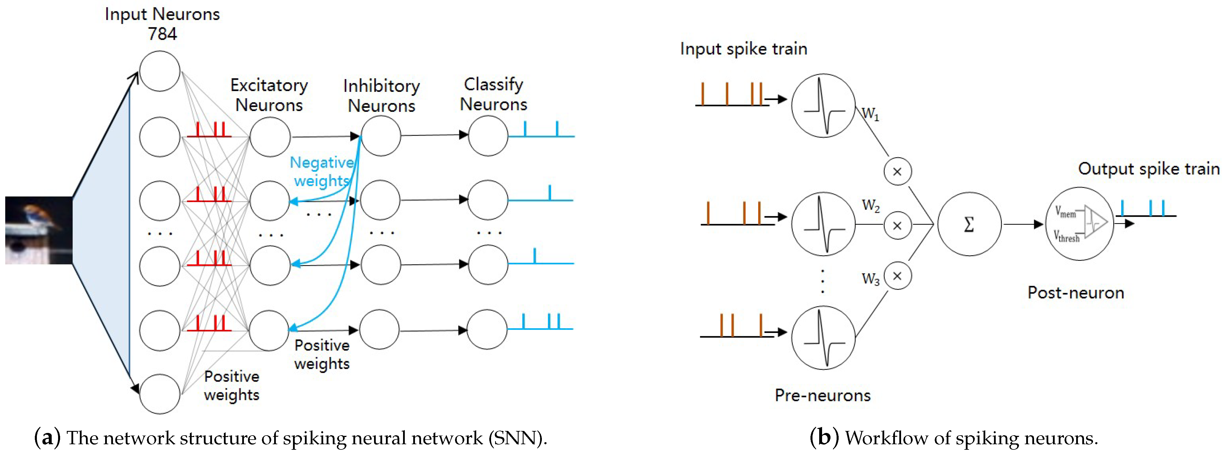
3.1. Neuron Model
3.2. Error Analysis
3.3. Initialize Membrane Potential
| Algorithm 1 Initialized membrane potential based on a trained ANN. |
|
| Algorithm 2 Initialized membrane potential based on training set. |
|
3.4. Coding Compensation
| Algorithm 3 Coding compensation. |
|
4. Experiments
4.1. Experiment Preparation
4.1.1. Experiment Environment
4.1.2. Pre-Processing
4.1.3. Hyper-Parameters
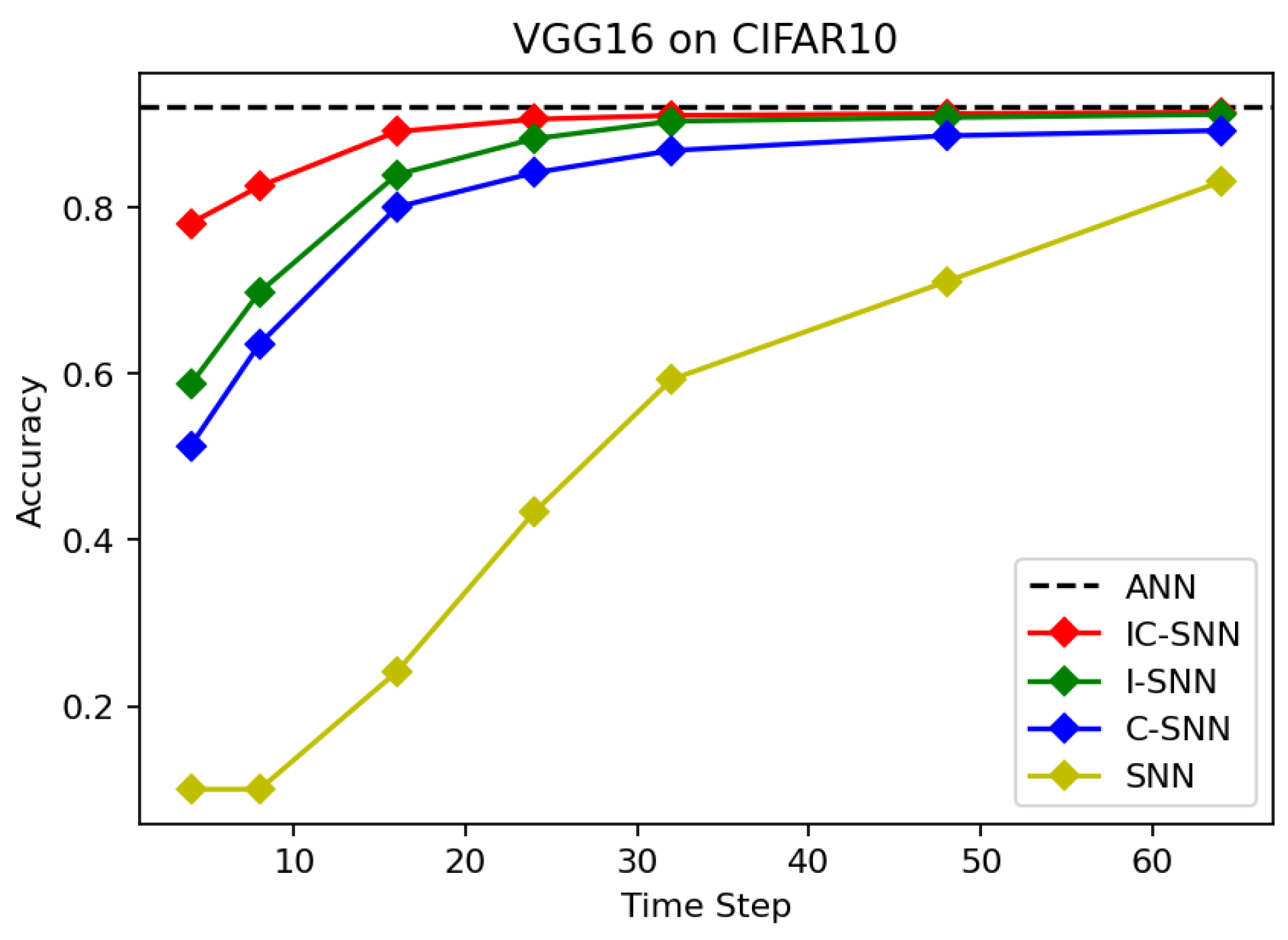
4.2. Validity Verification
4.2.1. Accuracy
4.2.2. Fire Time
4.2.3. Output
4.3. Contrast Experiment
5. Conclusions
Author Contributions
Funding
Institutional Review Board Statement
Informed Consent Statement
Data Availability Statement
Conflicts of Interest
References
- Guo, Y.; Yao, A.; Chen, Y. Dynamic network surgery for efficient dnns. arXiv 2016, arXiv:1608.04493. [Google Scholar]
- Gong, Y.; Liu, L.; Yang, M.; Bourdev, L. Compressing deep convolutional networks using vector quantization. arXiv 2014, arXiv:1412.6115. [Google Scholar]
- Han, S.; Mao, H.; Dally, W.J. Deep compression: Compressing deep neural networks with pruning, trained quantization and huffman coding. arXiv 2015, arXiv:1510.00149. [Google Scholar]
- Gerstner, W.; Kistler, W.M. Spiking Neuron Models: Single Neurons, Populations, Plasticity; Cambridge University Press: Cambridge, UK, 2002. [Google Scholar] [CrossRef] [Green Version]
- Attwell, D.; Laughlin, S.B. An energy budget for signaling in the grey matter of the brain. J. Cereb. Blood Flow Metab. 2001, 21, 1133–1145. [Google Scholar] [CrossRef]
- Maass, W.; Markram, H. On the computational power of circuits of spiking neurons. J. Comput. Syst. Sci. 2004, 69, 593–616. [Google Scholar] [CrossRef] [Green Version]
- Song, S.; Miller, K.D.; Abbott, L.F. Competitive Hebbian learning through spike-timing-dependent synaptic plasticity. Nat. Neurosci. 2000, 3, 919–926. [Google Scholar] [CrossRef]
- Hebb, D.O. The Organization of Behavior: A Neuropsychological Theory; Psychology Press: New York, NY, USA, 2005. [Google Scholar] [CrossRef]
- Zhang, T.; Cheng, X.; Jia, S.; Poo, M.m.; Zeng, Y.; Xu, B. Self-backpropagation of synaptic modifications elevates the efficiency of spiking and artificial neural networks. Sci. Adv. 2021, 7, eabh0146. [Google Scholar] [CrossRef]
- Rumelhart, D.E.; Hinton, G.E.; Williams, R.J. Learning representations by back-propagating errors. Nature 1986, 323, 533–536. [Google Scholar] [CrossRef]
- Bohte, S.M.; Kok, J.N.; La Poutre, H. Error-backpropagation in temporally encoded networks of spiking neurons. Neurocomputing 2002, 48, 17–37. [Google Scholar] [CrossRef] [Green Version]
- Wu, Y.; Deng, L.; Li, G.; Zhu, J.; Shi, L. Spatio-temporal backpropagation for training high-performance spiking neural networks. Front. Neurosci. 2018, 12, 331. [Google Scholar] [CrossRef] [Green Version]
- Cao, Y.; Chen, Y.; Khosla, D. Spiking deep convolutional neural networks for energy-efficient object recognition. Int. J. Comput. Vis. 2015, 113, 54–66. [Google Scholar] [CrossRef]
- Bu, T.; Fang, W.; Ding, J.; Dai, P.; Yu, Z.; Huang, T. Optimal ANN-SNN Conversion for High-accuracy and Ultra-low-latency Spiking Neural Networks. In Proceedings of the International Conference on Learning Representations, Vienna, Austria, 30 April–3 May 2021. [Google Scholar]
- Wang, Z.; Lian, S.; Zhang, Y.; Cui, X.; Yan, R.; Tang, H. Towards Lossless ANN-SNN Conversion under Ultra-Low Latency with Dual-Phase Optimization. arXiv 2022, arXiv:2205.07473. [Google Scholar]
- Masquelier, T.; Thorpe, S.J. Unsupervised learning of visual features through spike timing dependent plasticity. PLoS Comput. Biol. 2007, 3, e31. [Google Scholar] [CrossRef] [PubMed] [Green Version]
- Legenstein, R.; Pecevski, D.; Maass, W. A learning theory for reward-modulated spike-timing-dependent plasticity with application to biofeedback. PLoS Comput. Biol. 2008, 4, e1000180. [Google Scholar] [CrossRef] [Green Version]
- Ruf, B.; Schmitt, M. Learning temporally encoded patterns in networks of spiking neurons. Neural Process. Lett. 1997, 5, 9–18. [Google Scholar] [CrossRef]
- Wade, J.J.; McDaid, L.J.; Santos, J.A.; Sayers, H.M. SWAT: An unsupervised SNN training algorithm for classification problems. In Proceedings of the 2008 IEEE International Joint Conference on Neural Networks (IEEE World Congress on Computational Intelligence), Hong Kong, China, 1–6 June 2008; pp. 2648–2655. [Google Scholar] [CrossRef]
- Diehl, P.U.; Cook, M. Unsupervised learning of digit recognition using spike-timing-dependent plasticity. Front. Comput. Neurosci. 2015, 9, 99. [Google Scholar] [CrossRef] [Green Version]
- Tavanaei, A.; Maida, A.S. Bio-inspired spiking convolutional neural network using layer-wise sparse coding and STDP learning. arXiv 2016, arXiv:1611.03000. [Google Scholar]
- Zhang, T.; Zeng, Y.; Zhao, D.; Xu, B. Brain-inspired Balanced Tuning for Spiking Neural Networks. In Proceedings of the IJCAI, Stockholm, Swede, 13–19 July 2018; pp. 1653–1659. [Google Scholar]
- Wu, Y.; Deng, L.; Li, G.; Zhu, J.; Xie, Y.; Shi, L. Direct training for spiking neural networks: Faster, larger, better. In Proceedings of the AAAI Conference on Artificial Intelligence, Honolulu, HI, USA, 8–12 October 2019; Volume 33, pp. 1311–1318. [Google Scholar] [CrossRef] [Green Version]
- Zhang, W.; Li, P. Temporal spike sequence learning via backpropagation for deep spiking neural networks. Adv. Neural Inf. Process. Syst. 2020, 33, 12022–12033. [Google Scholar] [CrossRef]
- Fang, W.; Yu, Z.; Chen, Y.; Masquelier, T.; Huang, T.; Tian, Y. Incorporating learnable membrane time constant to enhance learning of spiking neural networks. In Proceedings of the IEEE/CVF International Conference on Computer Vision, Montreal, QC, Canada, 10–17 October 2021; pp. 2661–2671. [Google Scholar] [CrossRef]
- Xiao, M.; Meng, Q.; Zhang, Z.; Wang, Y.; Lin, Z. Training feedback spiking neural networks by implicit differentiation on the equilibrium state. Adv. Neural Inf. Process. Syst. 2021, 34, 14516–14528. [Google Scholar]
- Diehl, P.U.; Neil, D.; Binas, J.; Cook, M.; Liu, S.C.; Pfeiffer, M. Fast-classifying, high-accuracy spiking deep networks through weight and threshold balancing. In Proceedings of the 2015 International Joint Conference on Neural Networks (IJCNN), Killarney, Ireland, 12–17 July 2015; pp. 1–8. [Google Scholar] [CrossRef]
- Rueckauer, B.; Lungu, I.A.; Hu, Y.; Pfeiffer, M.; Liu, S.C. Conversion of continuous-valued deep networks to efficient event-driven networks for image classification. Front. Neurosci. 2017, 11, 682. [Google Scholar] [CrossRef]
- Sengupta, A.; Ye, Y.; Wang, R.; Liu, C.; Roy, K. Going deeper in spiking neural networks: VGG and residual architectures. Front. Neurosci. 2019, 13, 95. [Google Scholar] [CrossRef] [PubMed] [Green Version]
- Kim, S.; Park, S.; Na, B.; Yoon, S. Spiking-yolo: Spiking neural network for energy-efficient object detection. In Proceedings of the AAAI Conference on Artificial Intelligence, New York, NY, USA, 7–12 February 2020; Volume 34, pp. 11270–11277. [Google Scholar] [CrossRef]
- Park, S.; Kim, S.; Na, B.; Yoon, S. T2FSNN: Deep spiking neural networks with time-to-first-spike coding. In Proceedings of the 2020 57th ACM/IEEE Design Automation Conference (DAC), Virtual Event, 20–24 July 2020; pp. 1–6. [Google Scholar] [CrossRef]
- Han, B.; Roy, K. Deep spiking neural network: Energy efficiency through time based coding. In Proceedings of the European Conference on Computer Vision; Springer: Berlin/Heidelberg, Germany, 2020; pp. 388–404. [Google Scholar] [CrossRef]
- Stöckl, C.; Maass, W. Optimized spiking neurons can classify images with high accuracy through temporal coding with two spikes. Nat. Mach. Intell. 2021, 3, 230–238. [Google Scholar] [CrossRef]
- Han, B.; Srinivasan, G.; Roy, K. Rmp-snn: Residual membrane potential neuron for enabling deeper high-accuracy and low-latency spiking neural network. In Proceedings of the IEEE/CVF Conference on Computer Vision and Pattern Recognition, Seattle, WA, USA, 13–19 June 2020; pp. 13558–13567. [Google Scholar]
- Deng, S.; Gu, S. Optimal conversion of conventional artificial neural networks to spiking neural networks. arXiv 2021, arXiv:2103.00476. [Google Scholar]
- Ding, J.; Yu, Z.; Tian, Y.; Huang, T. Optimal ann-snn conversion for fast and accurate inference in deep spiking neural networks. arXiv 2021, arXiv:2105.11654. [Google Scholar]
- Rathi, N.; Srinivasan, G.; Panda, P.; Roy, K. Enabling deep spiking neural networks with hybrid conversion and spike timing dependent backpropagation. arXiv 2020, arXiv:2005.01807. [Google Scholar]
- Bu, T.; Ding, J.; Yu, Z.; Huang, T. Optimized Potential Initialization for Low-latency Spiking Neural Networks. arXiv 2022, arXiv:2202.01440. [Google Scholar] [CrossRef]
- Delorme, A.; Gautrais, J.; Van Rullen, R.; Thorpe, S. SpikeNET: A simulator for modeling large networks of integrate and fire neurons. Neurocomputing 1999, 26, 989–996. [Google Scholar] [CrossRef]
- Simonyan, K.; Zisserman, A. Very deep convolutional networks for large-scale image recognition. arXiv 2014, arXiv:1409.1556. [Google Scholar]
- He, K.; Zhang, X.; Ren, S.; Sun, J. Deep residual learning for image recognition. In Proceedings of the IEEE Conference on Computer Vision and Pattern Recognition, Las Vegas, NV, USA, 27–30 June 2016; pp. 770–778. [Google Scholar] [CrossRef]


| Symbol | Definition |
|---|---|
| l | Layer index |
| Input in ANN | |
| Weight in ANN and SNN | |
| Bias in ANN and SNN | |
| Activation function in ANN | |
| t | Time step |
| T | Simulation time step |
| The spike sequence, consisting of 0 and 1 | |
| Temporary membrane potential at time t | |
| Membrane potential at time t | |
| Threshold | |
| The spiking state of neurons at time t | |
| Spike fire rate |
| [28] | − | ||||||
| [29] | − | − | − | − | − | ||
| [37] | − | − | − | − | |||
| [34] | − | − | |||||
| [32] | − | − | − | ||||
| [35] | − | − | |||||
| [36] | − | ||||||
| [29] | − | − | − | − | − | ||
| [34] | − | − | − | − | |||
| [32] | − | − | − | − | |||
| [35] | − | − | |||||
Disclaimer/Publisher’s Note: The statements, opinions and data contained in all publications are solely those of the individual author(s) and contributor(s) and not of MDPI and/or the editor(s). MDPI and/or the editor(s) disclaim responsibility for any injury to people or property resulting from any ideas, methods, instructions or products referred to in the content. |
© 2022 by the authors. Licensee MDPI, Basel, Switzerland. This article is an open access article distributed under the terms and conditions of the Creative Commons Attribution (CC BY) license (https://creativecommons.org/licenses/by/4.0/).
Share and Cite
Li, C.; Shang, Z.; Shi, L.; Gao, W.; Zhang, S. IC-SNN: Optimal ANN2SNN Conversion at Low Latency. Mathematics 2023, 11, 58. https://doi.org/10.3390/math11010058
Li C, Shang Z, Shi L, Gao W, Zhang S. IC-SNN: Optimal ANN2SNN Conversion at Low Latency. Mathematics. 2023; 11(1):58. https://doi.org/10.3390/math11010058
Chicago/Turabian StyleLi, Cuixia, Zhiquan Shang, Li Shi, Wenlong Gao, and Shuyan Zhang. 2023. "IC-SNN: Optimal ANN2SNN Conversion at Low Latency" Mathematics 11, no. 1: 58. https://doi.org/10.3390/math11010058