Article

Motion-Compensated PET Image Reconstruction via Separable Parabolic Surrogates

by
Nicholas E. Protonotarios
1,*,
George A. Kastis
2,3,
Andreas D. Fotopoulos
4,
Andreas G. Tzakos
5,
Dimitrios Vlachos
6 and
Nikolaos Dikaios
2
1
Department of Applied Mathematics and Theoretical Physics, University of Cambridge, Cambridge CB3 0WA, UK
2
Mathematics Research Center, Academy of Athens, 11527 Athens, Greece
3
Institute of Nuclear and Radiological Science and Technology, Energy and Safety (INRASTES), National Center for Scientific Research “Demokritos”, 15310 Agia Paraskevi, Greece
4
Neurosurgical Institute, University of Ioannina, 45500 Ioannina, Greece
5
Section of Organic Chemistry and Biochemistry, Department of Chemistry, University of Ioannina, 45110 Ioannina, Greece
6
Department of Economics, University of Peloponnese, 22100 Tripoli, Greece
*
Author to whom correspondence should be addressed.
Mathematics 2023, 11(1), 55; https://doi.org/10.3390/math11010055
Submission received: 11 November 2022 / Revised: 13 December 2022 / Accepted: 20 December 2022 / Published: 23 December 2022
(This article belongs to the Topic Mathematical Modeling in Physical Sciences)

Abstract

:
The effective resolution of positron emission tomography (PET) can be significantly degraded by patient motion during data acquisition. This is especially true in the thorax due to respiratory motion. This study concentrates on the improvement of motion correction algorithms both in terms of image quality and computational cost. In this paper, we present a novel motion-compensated image reconstruction (MCIR) algorithm based on a parabolic surrogate likelihood function instead of the loglikelihood function of the expectation maximization (EM) algorithm. The theoretical advantage of the parabolic surrogate algorithm lies within the fact that its loglikelihood is upper bounded by the EM loglikelihood, thus it will converge faster than EM. This is of particular importance in PET motion correction, where reconstructions are very computationally demanding. Relaxation parameters were also introduced to converge closer to the maximum likelihood (ML) solution and achieve lower noise levels. Image reconstructions with embedded relaxation parameters actually converged to better solutions than the corresponding ones without relaxation. Motion-compensated parabolic surrogates were indeed shown to accelerate convergence compared to EM, without reaching a limit cycle. Nonetheless, with the incorporation of ordered subsets in the reconstruction setting, the improvement was less evident.

1. Introduction

In positron emission tomography (PET) image reconstruction, patient motion, particularly due to respiration, frequently causes significant image degradation and blurring [1]. In the course of respiration, air is inhaled and exhaled, resulting in the contraction and expansion of the patient’s lungs, as well as the movement of other organs in the thoracic region. Furthermore, respiration leads to a potential loss of contrast in the images, often accounting for the failure to detect lesions and the degradation of accuracy of image quantification [2]. Since the amplitude of respiratory motion can be up to 30 mm, respiratory motion may dominate PET images, whereas the spatial resolution of commercial whole-body PET scanners utilizing silicon photomultipliers is typically 3–4 mm [3].
To overcome the above limitations, there exist several motion correction techniques [4,5,6,7]. These techniques include respiratory-gated PET acquisition protocols [8], especially focusing on motion blurring, and motion compensation and correction methods prior to image reconstruction, for the gated data acquired [9,10]. However, the incorporation of motion within the algorithm itself occurs in the “motion-compensated image reconstruction” (MCIR) algorithms [11,12,13]. In this direction, it is quite common to co-register reconstructed images by employing post-reconstruction registration (PRR), i.e., by splitting the projection data, depending on the motion phase, into gated data (sinograms). The resulting gated sinograms are reconstructed separately and the images are registered to a reference phase and are subsequently averaged [14,15,16,17]. MCIR methods include joint estimation of image and deformation parameters [18], model-based image reconstruction for four-dimensional PET [19], motion-incorporated reconstructions for gated PET [20], lesion detectability in respiratory-gated PET/CT (computed tomography) [21], the incorporation of non-rigid body transformations [22], respiratory motion compensation [23], and expectation maximization (EM) algorithms [24], proven to form the basis of MCIR.
MCIR is often employed to alleviate motion in several clinical applications. This is especially true with the recent integration of PET with magnetic resonance imaging (MRI), where motion is measured jointly with PET and MRI [25]. In this case, MCIR techniques are utilized for respiratory motion correction [26,27,28] and for several other types of motion correction [29,30]. Furthermore, some researchers have focused on PET motion correction via convolutional neural networks [31] and adversarial networks [32], and several others on the noise properties of MCIR [33].
A significant drawback involved in EM reconstruction is the associated computational expense. However, the application of iterative EM algorithms in PET image reconstruction is prevalent. There exist several EM-based reconstruction techniques, including ordered subsets EM (OSEM) [34], one-step-late expectation maximization [35], space-alternating generalized expectation maximization (SAGE) [36], and separable parabolic surrogates (SPS) [37]. The parabolic surrogate algorithm was shown to converge faster than maximum likelihood EM (MLEM) and SAGE [37].
In this paper, following the works by Fessler and Erdogan [37] and Dikaios [38], we investigate the use of motion-compensated image reconstruction, based on an SPS likelihood function instead of the usual loglikelihood function of the EM algorithm. The loglikelihood of the proposed SPS algorithm is upper bounded by the EM loglikelihood, thus it will converge faster. Furthermore, we extended our technique by incorporating the notion of ordered subsets (OS) and relaxation parameters. The research gap that this article fills is the improvement of the convergence rate, which is crucial in order to reduce the computational cost involved in PET image reconstruction.
The current paper is organized as follows: in Section 2, we describe the basics of EM image reconstruction. In Section 3, we illustrate parabolic surrogates image reconstruction, whereas in Section 4 we highlight motion-compensated EM image reconstruction. Furthermore, in Section 5 we present our proposed framework, namely motion-compensated SPS image reconstruction. In Section 6, we present the numerical implementation and the results of our novel method and in Section 7 we discuss our results. Finally, in Section 8 we provide our conclusions.

2. Maximum Likelihood Expectation Maximization Image Reconstruction

EM algorithms adopt iterative approaches to compute maximum likelihood (ML) estimates of unknown parameters ( λ ), given the measured data (y) [39]. ML estimates aim to find the parameters for which the measured data are the most likely. However, missing or unobserved data (x) may be included in the EM scheme. The terms “missing data” or “unobserved data” imply that there exist sample spaces X and Y, and a mapping x y ( x ) from X to Y. The measured data y consist of a realization from space Y, whereas the missing data x are observed indirectly through the mapping y = y ( x ) . If we assume that the conditional probability of the missing data x given λ is P ( x | λ ) , then we are able to calculate the conditional probability of the observed data P ( y | λ ) . It is important to note that there might be more than one realization x X that will generate P ( y | λ ) .
In EM algorithms, we aim to maximize P ( y | λ ) , which, via the definition of conditional probability, may be rewritten as:
P ( y | λ ) = x P ( y | x , λ ) P ( x | λ ) .
As it is quite often in these cases, instead of the likelihood P ( y | λ ) , given in Equation (1), the loglikelihood function L ( y | λ ) is employed, namely,
L ( y | λ ) = ln P ( y | λ ) ,
since the loglikelihood is usually more convenient to maximize. The natural logarithm is monotonically increasing, hence, if λ * denotes the estimate that maximizes P ( y | λ ) , it follows that it will also maximize L ( y | λ ) , i.e.,
λ * = arg max λ P ( y | λ ) = arg max λ L ( y | λ ) .
In order to converge to the maximum likelihood solution, each updated EM estimate, denoted by λ n , must monotonically increase the loglikelihood function, in the sense that:
L ( y | λ ) > L ( y | λ n ) , n .
To this end, EM algorithms usually consist of two steps per iteration, namely: (i) the expectation step (E-step), estimating the missing data with their expected values, given the current value of λ and y; (ii) the maximization step (M-step), calculating the ML estimates of the unknown parameters, and subsequently utilizing them in the next E-step.
In the context of PET imaging, the aim is to reconstruct the radioactivity distribution which is the most likely. Following data acquisition, a PET scanner provides projection (observed) data, y, of the radioactivity distribution. Then, the EM algorithm is employed in order to determine a radioactivity distribution λ that maximizes the conditional expectation Q ( y | λ n ) , i.e.,
Q ( y | λ n ) = E L ( x | λ ) | y , λ n ,
as in [37,40,41]. Since the reconstruction is performed in a discrete setting, the projection data are modeled as geometrically ordered arrays (usually referred to as sinograms), denoted by y b , where b represents the bin corresponding to a line of response [42]. In a similar fashion, the radioactivity distribution function is represented as the radioactivity concentration λ v , in each voxel v [43].
The probability of detecting y b photons according to Poisson statistics is
P ( y b | λ v ) = e y ¯ b y ¯ b y b y b ! ,
where the estimated (mean) projection data, y ¯ b is represented by
y ¯ b = v p b v λ v ,
where p b v denotes the probability that a photon from image voxel v is actually detected in the sinogram bin b. Given the observed data y b , the likelihood function of the radioactivity distribution λ v is given by
P ( y | λ ) = b P ( y b | λ ) ,
in the sense of [40,41]. Incorporating the loglikelihood ( L ) into Equation (8) yields
L ( y | λ ) = b y b ln y ¯ b y ¯ b ln y ¯ b ! .
In Equation (9), we omit the term ln y ¯ b ! , as it contributes nothing in the loglikelihood maximization process, i.e.,
L ( y | λ ) = b y b ln y ¯ b y ¯ b .
PET projection data ( y b ) contain insufficient information regarding the exact location, along the projection line, the photon annihilation event has occurred, hence they do not correspond to the complete dataset. To adequately define the EM algorithm [39], we must estimate a conditional expectation of the complete data ( x b v ), namely E ( x b v | y b , λ v ) , where x b v denotes the number of photons in voxel v detected in detector b. The complete data have an expected (mean) value of:
E ( x b v ) = p b v λ v ,
whereas the estimated observed projection data is calculated via the sum of the expectations given in Equation (11), over the voxels (v):
y ¯ b = v E ( x b v ) .

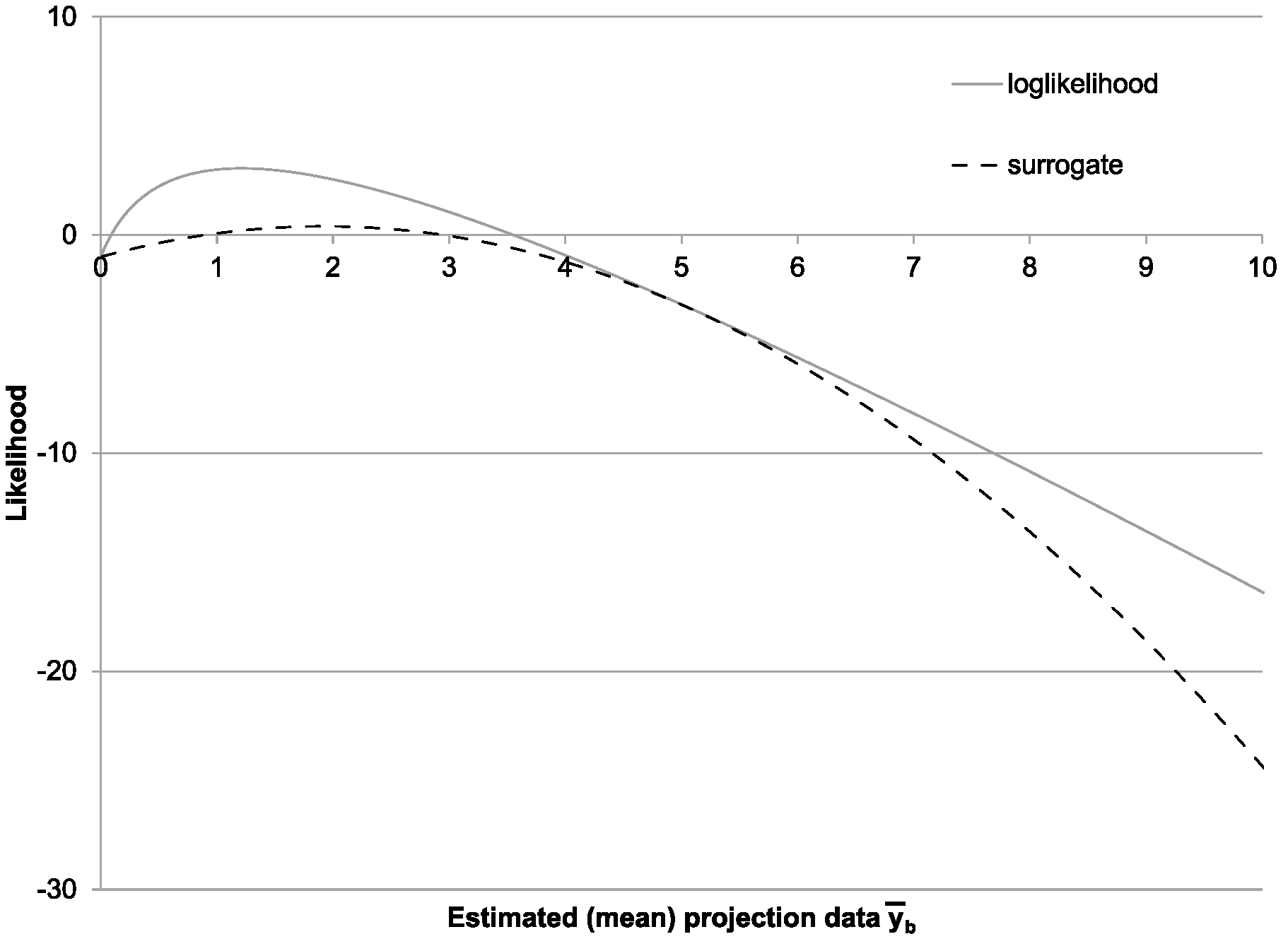
3. Parabolic Surrogates Image Reconstruction

SPS algorithms [37] are conceptually similar to SAGE algorithms [36], aiming for fast global convergence. In SAGE, convergence is achieved via a less informative, complete data set to the likelihood function [36]. The updated likelihood function in SAGE can be taken into account as a so-called “surrogate function”. In this direction, SPS algorithms replace the EM likelihood function with a parabolic surrogate function that is guaranteed to be monotonic even with non-zero background ( m b ).
Given the measured data y b , the loglikelihood function of the estimated parameters λ v is
L ( y | λ ) = b y b ln v p b v λ v + m b v p b v λ v m b .
Equation (13) may be rewritten in the following form:
L ( y | λ ) = b L b ( y b | λ ) ,
where
L b ( y b | λ ) = y b ln y ¯ b + m b y ¯ b + m b ,
and the mean projected data, y ¯ b , are defined in Equation (7).
The function L b ( y b | λ ) satisfies the following five conditions:
L b ( y b | λ ) y b ln y b y b , y ¯ b 0 ,
L b ( y b | λ ) increases monotonically in [ , y b ] ,
L b ( y b | λ ) decreases monotonically in ( y b , ) ,
L b ( y b | λ ) is concave in [ 0 , ) ,
L b ( y b | λ ) y b is convex in [ 0 , ) .
Conditions (16) imply, via Equation (14), that the loglikelihood function L ( y | λ ) is monotonically increasing.
Initially, the one-dimensional parabolic surrogate functions, denoted by ϕ b ( y ¯ b | y ¯ b n ) , are calculated as follows:
ϕ b ( y ¯ b | y ¯ b n ) = L b ( y ¯ b | λ n ) + y ¯ b y ¯ b n L b ( y ¯ b | λ n ) y ¯ b n 1 2 c b ( y ¯ b n ) y ¯ b y ¯ b n 2 ,
where c b ( y ¯ b n ) represents the curvature, as in [37], i.e.,
c b ( y ¯ b n ) = 2 y ¯ b 2 L b ( y b | λ ) y b ln m b + m b y ¯ b L b ( y b | λ ) y ¯ b , y ¯ b > 0 , 2 L b ( y b | λ ) y ¯ b 2 , y ¯ b = 0 .
The sum of the one-dimensional parabolic surrogate functions ϕ b ( y ¯ b | y ¯ b n ) gives the total parabolic surrogate function, denoted by Φ :
Φ ( λ | λ n ) = b ϕ b ( y ¯ b | y ¯ b n ) .
In the M-step of the EM algorithm, the parabolic surrogate function Φ is maximized:
λ n + 1 = arg max λ Φ ( λ | λ n ) .
In Equation (20), in order for the updated λ to monotonically increase the loglikelihood function L ( y | λ ) , the one-dimensional parabolic surrogate functions must satisfy the following three conditions, namely
ϕ b ( y ¯ b | y ¯ b n ) = L b ( y b , λ n ) ,
ϕ b ( y ¯ b | y ¯ b n ) y ¯ b n = L b ( y b | λ n ) y ¯ b n ,
ϕ b ( y ¯ b | y ¯ b n ) L b ( y b , λ ) , y ¯ b 0 .
As shown in Figure 1, Equation (19) and conditions (21) imply that the parabolic surrogate function Φ : (i) is bounded above by the typical loglikelihood function L , and (ii) has the same value and the same slope with L only when y ¯ b = y ¯ b n .

4. Motion-Compensated Expectation Maximization Image Reconstruction

Depending on the motion phase (m), in gated sinograms y m , the probability of detecting y b m events (photons) in projection element b for gate m from a radioactivity distribution λ v is governed by Poisson statistics, as in Equation (6), namely:
P ( y b m | λ v ) = e y ¯ b m y ¯ b m y b m y b m ! ,
where y ¯ b m denotes the estimated (mean) projection data of a projection element b for gate m.
In PRR, the reconstructed image of each gate m, denoted by λ m , is deformed by its corresponding transformation operator, T. Then, an average image of the M deformed and resampled images is formed. The motion of the radioactivity distribution from its initial position, i.e., gate 1, to gate m is represented by
λ v m = v d v v 1 m λ v ,
where d 1 m denotes the elements of the transformation matrix T that transform the image from respiratory gate 1 to gate m. Therefore, the estimated (mean) projection data for gate m will be
y ¯ b m = v p b v v d v v 1 m λ v ,
where p b v is the probability that a photon from image voxel v is detected in sinogram bin b. For the calculation of the estimated projection data that are consistent with the measured data, we assume perfect deformation for each gate. We adapt the loglikelihood function given by Shepp and Vardi [40], and rewrite the motion-gated case as:
L ( y | λ ) = m b y b m ln y ¯ b m y ¯ b m .
Using Equation (24), Equation (25) may be written as [19]
L ( y | λ ) = m b y b m ln v p b v v d v v 1 m λ v v p b v v d v v 1 m λ v .
For the determination of the E-step of the EM algorithm, we must estimate the conditional expectation of the complete data, x b v m , denoted by E ( x b v m | y b m , λ v ) , as in [39]. Since x b v m are independent Poisson variables with mean values p b v λ v m , it follows that
E ( x b v m | y b m , λ v ) = y b m p b v λ v m v p b v λ v m = y b m p b v v d v v 1 m λ v v p b v λ v m .
The conditional expectation, Q ( λ v | λ v n ) , where λ v n denotes the value of λ v at iteration n of the EM algorithm, is given by
Q ( λ v | λ v n ) = E L ( x , λ ) | y , λ n = m b p b v v d v v 1 m λ v + E x b v m | y b m , λ v n ln p b v v d v v 1 m λ v .
Furthermore, we assume that the deformation of the probability matrix can replace the deformation of the radioactivity distribution, i.e.,
λ v v d v v 1 m p b v = p b v v d v v 1 m λ v .
Therefore, Equation (28) may be rewritten as
Q ( λ v | λ v n ) = m b λ v v d v v m 1 p b v + E x b v m | y b m , λ v n ln λ v v d v v m 1 p b v .
For the determination of the M-step of the EM algorithm, we seek the image for which the conditional expectation is maximized, i.e.,
Q ( λ v | λ v n ) λ v = 0 ,
which, via Equation (30), implies that
m b v d v v m 1 p b v + E x b v m | y b m , λ v n λ v = 0 .
Therefore, the image update equation will be
λ v n + 1 = m b E x b v m | y b m , λ v n m b v d v v m 1 p b v .
Substituting Equation (29) into the numerator of Equation (27) yields
E ( x b v m | y b m , λ v n ) = λ v n y b m v d v v m 1 p b v v p b v v d v v 1 m p b v λ v n .
Further substitution of Equation (34) into Equation (33) implies that the image update equation will have the following form:
λ v n + 1 = λ v n 1 m v d v v m 1 b p b v m v d v v m 1 b y b m v p b v v d v v 1 m λ v .
The term inside the brackets in the right-hand-side of Equation (35) will be referred to as the image estimate update factor. This update factor is the product of the sensitivity correction term and the back-projected ratio. If we consider to include photon attenuation, in the form of an attenuation factor matrix denoted by A b m , and ordered subsets, denoted by S i , then Equation (35) becomes
λ v n + 1 = λ v n 1 m v d v v m 1 b S i p b v A b m m v d v v m 1 b S i y b m v p b v v d v v 1 m λ v .
Equation (36) represents the image update equation for MCIR, taking into account photon attenuation (in the form of an attenuation factor matrix denoted by A b m , and ordered subsets, denoted by S i ). This means that the updated image λ v n + 1 is λ v n multiplied by the “update factor”, i.e., the product of the sensitivity correction term and the back-projected ratio.

5. Motion-Compensated Separable Parabolic Surrogates Image Reconstruction

MCIR methods, described in the previous section, are usually computationally costly. In order for an MCIR method to be clinically applicable, the computational cost must be reduced. Ordered subsets may accelerate the convergence significantly, however, this occurs at the expense of reaching a limit cycle at early iterations. As mentioned in the introduction, there exist several methods that are able to accelerate the EM process and maintain convergence to the maximum likelihood solution. One of these methods is SPS, proposed by Erdogan and Fessler [37]. SPS improves the convergence rate while maintaining the important monotonic properties of the EM algorithm. In SPS, the loglikelihood function is replaced by a separable parabolic surrogate.
Given that SPS was proven to converge faster than the SAGE algorithm [36,37], in this section we introduce two motion-compensated parabolic surrogates reconstruction methods, namely MC-SPS (motion-compensated SPS) and MC-OSSPS (motion-compensated, ordered-subsets SPS). In both reconstruction methods, the motion model is embedded within the parabolic surrogate function.

5.1. MC-SPS: Motion-Compensated Separable Parabolic Surrogates Image Reconstruction

Following the notions of SPS and MCIR, as scrutinized above, we modify the one-dimensional parabolic surrogate functions ϕ b , given in Equation (17), in order to obtain ϕ b m for each gate m, as follows:
ϕ b m ( y ¯ b m | y ¯ b m n ) = L b m ( y ¯ b m | λ n ) + ( y ¯ b m y ¯ b m n ) L b m ( y ¯ b m | λ n ) y ¯ b m n 1 2 c b m ( y ¯ b m n ) ( y ¯ b m y ¯ b m n ) 2 ,
where c b m ( y ¯ b m n ) denotes the curvature, initially defined in [37], and modified from Equation (18) for gate m, namely:
c b m ( y ¯ b m n ) = 2 ( y ¯ b m ) 2 L b m ( y b m | λ ) y b m ln m b + m b y ¯ b m L b m ( y b m | λ ) y ¯ b m , y ¯ b m > 0 , 2 L b m ( y b m | λ ) ( y ¯ b m ) 2 , y ¯ b = 0 ,
y ¯ b m denotes the estimated projection data for gate m, i.e.,
y ¯ b m = v p b v λ v m ,
and L b m denotes the component of the loglikelihood function L b m corresponding to gate m:
L b m ( y m | λ ) = b y b m ln y ¯ b m y ¯ b m .
In order to obtain a surrogate function that is separable in v for all possible λ v , we applied the approach of De Pierro et al. [44]. For convenience, y ¯ b m via Equation (39) may be rewritten as
y ¯ b m = v p b v ( λ v m λ v m n ) + y ¯ b m n .
Furthermore, we assume that the deformation of the probability matrix can replace the corresponding deformation of the radioactivity distribution, as in Equation (23), i.e.,
p b v λ v m = p b v v d v v 1 m λ v λ v v d v v 1 m p b v .
Equation (42) implies that
p b v λ v m p b v λ v ,
hence, via Equation (43), Equation (41) is rewritten in the following form:
y ¯ b m = v p b v m p b m p b m ( λ v m λ v m n ) + y ¯ b m n ,
where
p b m = v p b v m .
However, given that ϕ b m ( y ¯ b m | y ¯ b m n ) is concave, hence
ϕ b m ( y ¯ b m | y ¯ b m n ) v p b v m p b m ϕ b m ( p b m ( λ v m λ v m n ) + y ¯ b m n | y ¯ b m n ) ,
due to the fact that Equations (44) and (45) define an affine combination, since
v p b v m p b m = 1 .
Inequality (47) yields a surrogate function Φ ˜ that is not only quadratic, but also separable in v:
Φ ˜ ( λ | λ n ) = m b v p b v m p b m ϕ b m ( p b m ( λ v m λ v m n ) + y ¯ b m n | y ¯ b m n ) .
For the M-step of our SPS algorithm, we must maximize these one-dimensional parabolas with respect to λ v :
ϕ ( λ | λ n ) λ v = m b p b v m L b m ( y b m | λ n ) y ¯ b m n + γ v n ( λ v λ v n ) = 0 ,
where γ v n is defined as
γ v n = m b p b v m p b m c b m ( y ¯ b m n ) ,
and the curvature c b m ( y ¯ b m n ) may be approximated via the Newton curvature [37,45], namely
c b m ( y ¯ b m ) = 2 L b m ( y b m | λ ) ( y ¯ b m ) 2 , y ¯ b m > 0 , 0 , otherwise .
Condition (49) implies
λ v n + 1 = λ v n 1 γ v n m b p b v m L b m ( y b m | λ n ) y ¯ b m n .
Under the above assumptions, the approximation provided by the MC-SPS algorithm is not guaranteed to be monotonic. However, as it will become apparent in the next subsection, the monotonicity violation will occur anyway, even when ordered subsets are introduced.

5.2. MC-OSSPS: Motion-Compensated Ordered-Subsets Separable Parabolic Surrogates Image Reconstruction

In order to further accelerate the convergence of MC-SPS, we employed the OS formulation [46], as we did in Equation (36), however, at the expense of global convergence. The resulting motion-compensated ordered subsets SPS algorithm (MC-OSSPS) is represented by:
λ v n + 1 = λ v n 1 γ v n m b S i p b v m L b m ( y b m | λ n ) y ¯ b m n ,
where OS are denoted by S i , as in Equation (36).
OS algorithms tend to converge faster than MLEM. However, in order to achieve acceleration, they employ an approximate gradient computed from a block of the projection data per iteration. OS-based methods are shown to reach a similar solution as MLEM, if the subsets are balanced and the degree of the projection subset subdivision is relatively low [38]. Given that the approximate gradient is not accurate, OS algorithms exhibit limit cycle behavior, producing periodic solutions. Hence they do not converge to the maximum likelihood solution, i.e., they violate global convergence. Since the magnitude of the limit cycle behavior is closely related to the step size, Browne and De Pierro [44] suggested the use of a relaxation parameter, corresponding to a diminishing step size, and proved that the new algorithm is indeed globally convergent. To this end, and in order to achieve better convergence we introduced a diminishing step size per iteration. The resulting, relaxed motion-compensated OSSPS (R-MC-OSSPS) algorithm is
λ v n + 1 = λ v n a n γ v n m b S i p b v m L b m ( y b m | λ n ) y ¯ b m n ,
where a n denotes the relaxation parameter. The diminishing nature of the step size requires that a n tends to zero, but not too rapidly:
lim n a n = 0 and n = 0 a n = .
If n = 0 a n < and the starting point of the OS algorithm is not close enough to the ML solution, the algorithm will never converge given that
λ v n + 1 λ v n 2 = O ( a n ) .
The notion of the relaxation parameter within the OS SPS framework was first introduced in [47], where Ahn and Fessler proved that global convergence is ensured when the following conditions are satisfied, namely,
n = 0 a n = ,
n = 0 a n 2 < ,
and
λ v n B o ,
where B o denotes the interior of the bounded set of solutions. The set B is such that B Λ , where Λ is given by:
Λ = λ v R + : L ( λ v ) > 0 ) .
In the present work, the preferred relaxation parameters were of the form:
a n = a 0 β n + 1 ,
with a 0 , β > 0 .

6. Numerical Implementation and Results

The proposed motion-compensated parabolic surrogates method was implemented on a desktop personal computer with a 2.50 GHz Intel® CoreTM i7-4710HQ CPU processor and 16 GB RAM operating memory, running Windows 10 Professional Edition. For the numerical implementation of our proposed algorithms, we employed a four-dimensional (4D), non-uniform rational B-spline cardiac-torso digital phantom (NCAT) [48]. The transformation operator for respiratory motion consisted of an affine and a non-rigid transformation to account for local deformations. For the non-rigid transformation, cubic B-splines were used because of their ability to model local deformations. The cost function minimized was mutual information, with the marginal and joint probability distributions determined using a Parzen window. To penalize local discontinuities in the transformation, a bending energy regularization term was included in the cost function. The algorithm used to minimize the cost function was the gradient descent. The optimization started with a sparse grid and moved to two finer resolutions. The NCAT CT images were registered, with the algorithm above [13] implemented using the ITK library [49] to determine seven deformation fields and their inverses. The motion gate used as a reference corresponded to the midpoint of the respiratory cycle to minimize the average motion between the reference gate and the rest of the gates.
Utilizing the NCAT phantom, motion-compensated SPS converged faster than motion-compensated MLEM; however, when combined with OS, the advantage was lost, namely the convergence of MC-OSSPS was similar to that of MC-OSEM. In order to ensure convergence of the MC-OSSPS case while avoiding the limit cycle, we investigated the use of a diminishing step size per iteration (relaxation).
Since SPS algorithms employ additive updates, the choice of the initial estimate may affect the convergence performance [47]. For the comparison of MC-OSSPS and R-MC-OSSPS, instead of a uniform initial estimate, we employed a reference gate image reconstructed using 60 MLEM iterations. Since the reference gate image was produced using data from a single gate, it was noisy, and subsequently it was smoothed with a 6 mm full width at half maximum (FWHM) Gaussian.
The motion-compensated SPS algorithms presented above were implemented within the SPS framework of STIR (Software for Tomographic Image Reconstruction) [50]. All images were reconstructed from span 3 data with a maximum ring difference of 11 into a 128 × 128 × 35 array, and with a voxel size of 3.125 × 3.125 × 4.25 mm. The approximate tube-of-response [13] back projector was employed for all algorithms in conjunction with line-of-response forward projection. Twelve subsets were utilized for all reconstructions and attenuation factors were applied in the corresponding probability matrix during the calculation of the sensitivity to correct for photon attenuation. Images with and without 6 mm FWHM Gaussian post-smoothing were produced. Furthermore, the relaxation parameters involved in Equation (59) for R-MC-OSSPS were chosen with the values of a 0 = 1 and β = 0.1 .
For the quality assessment of the images produced and for the examination of the convergence of the proposed algorithms, loglikelihood, and normalized loglikelihood functions were applied. Lesion percentage bias and contrast-to-noise ratio (CNR) were also employed for the evaluation of the algorithms.

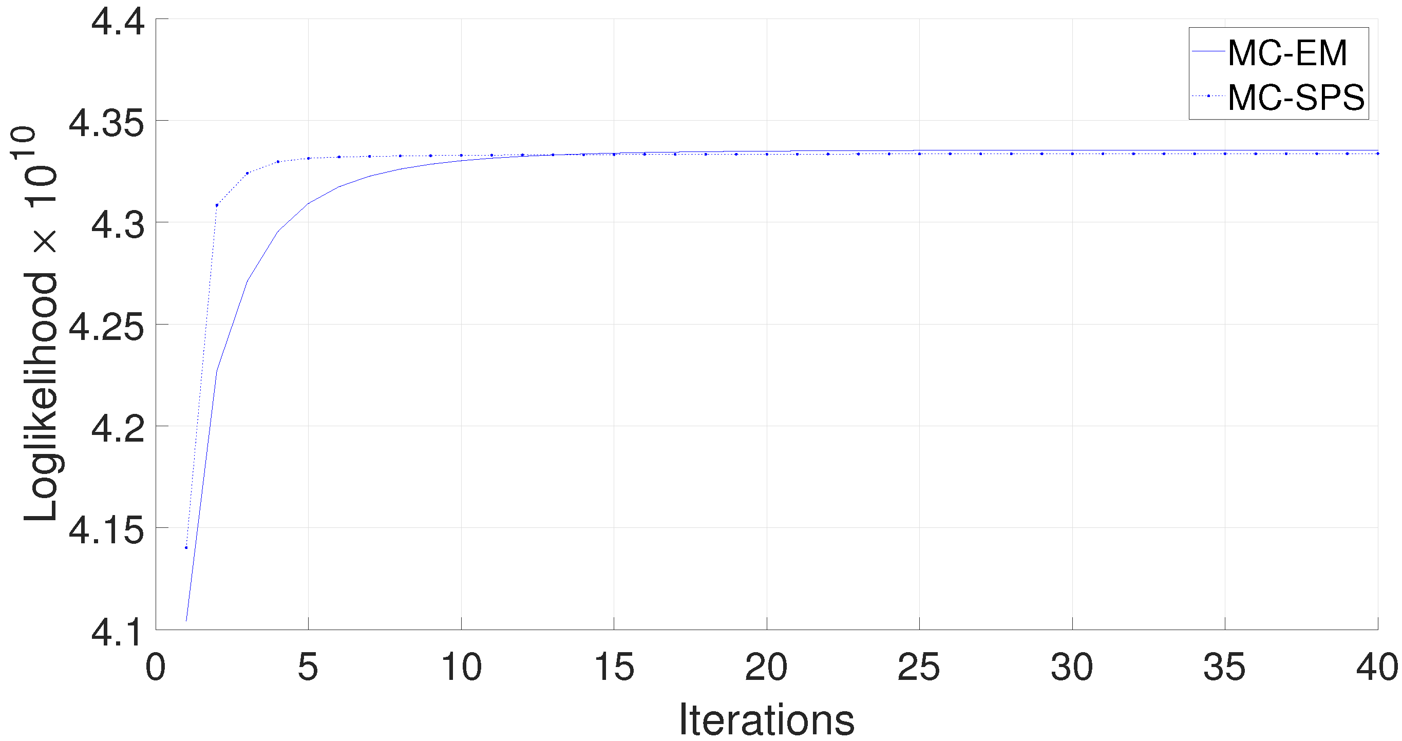
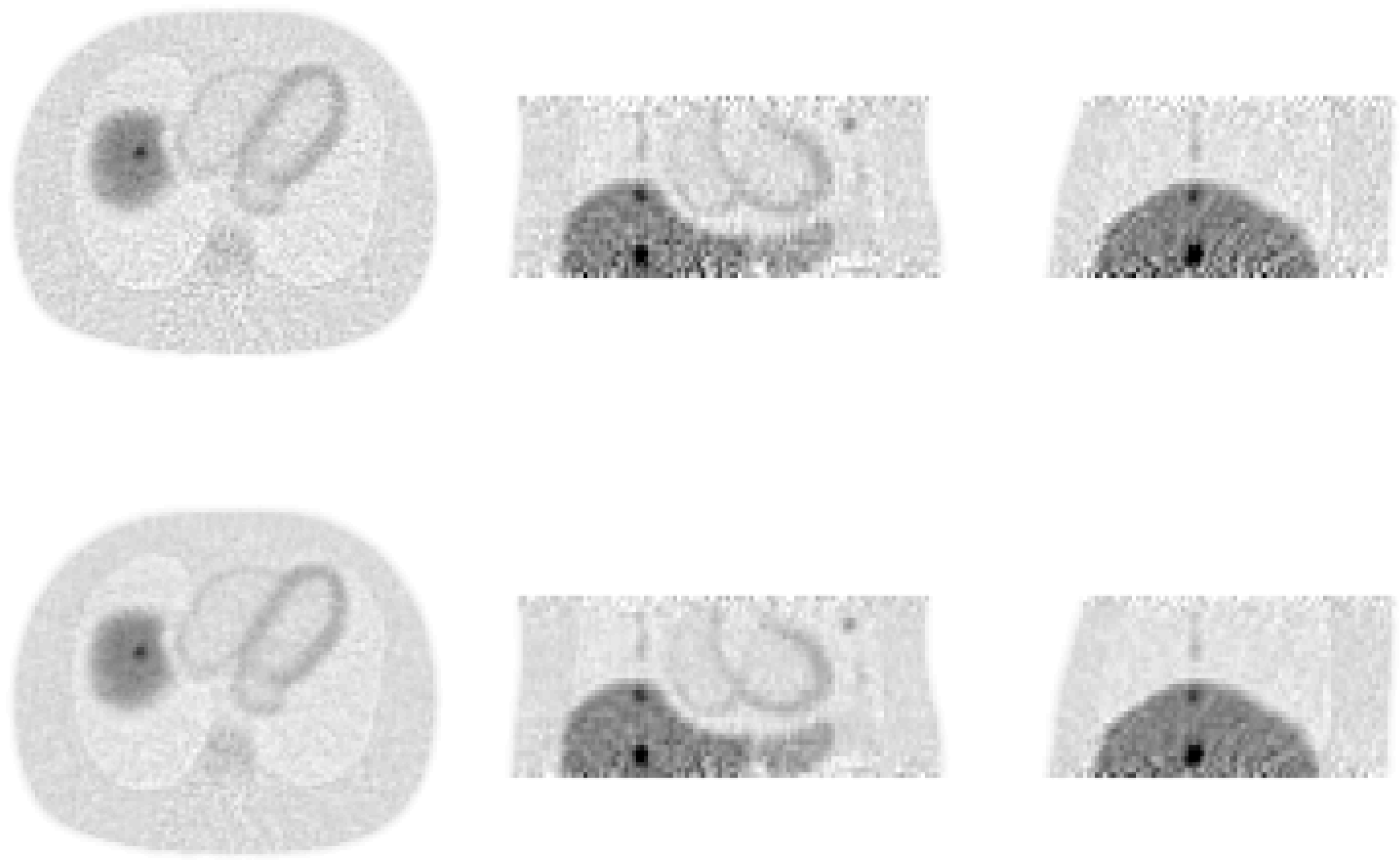
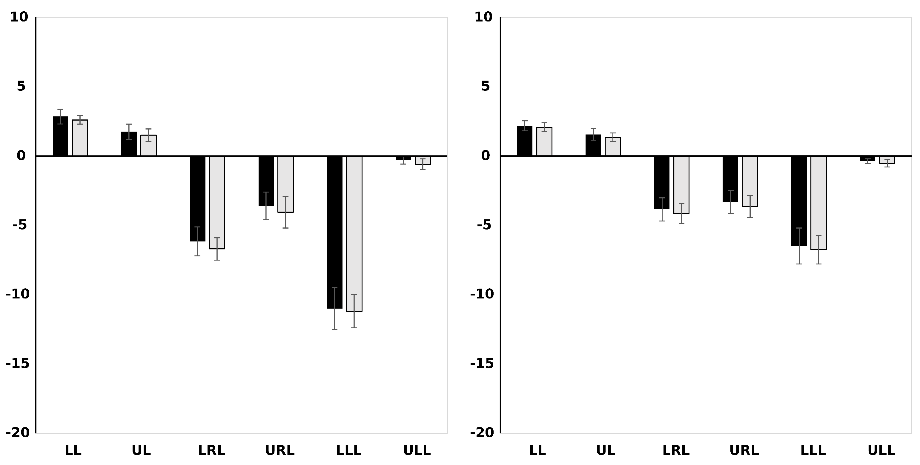
6.1. Comparison of Motion-Compensated SPS and EM Algorithms

Figure 2 illustrates the convergence for motion-compensated SPS (MC-SPS) and the corresponding motion-compensated EM (MC-EM) algorithm, represented by Equation (35), incorporating photon attenuation. The parabolic surrogate function increased the loglikelihood more rapidly; this fact is in agreement with [37]. MC-OSSPS converged slightly faster than MC-OSEM, considering the same number of subsets (in this case 12); however, the acceleration advantage was negligible; see Figure 3. Both algorithms reached a limit cycle at a relatively low iteration number.

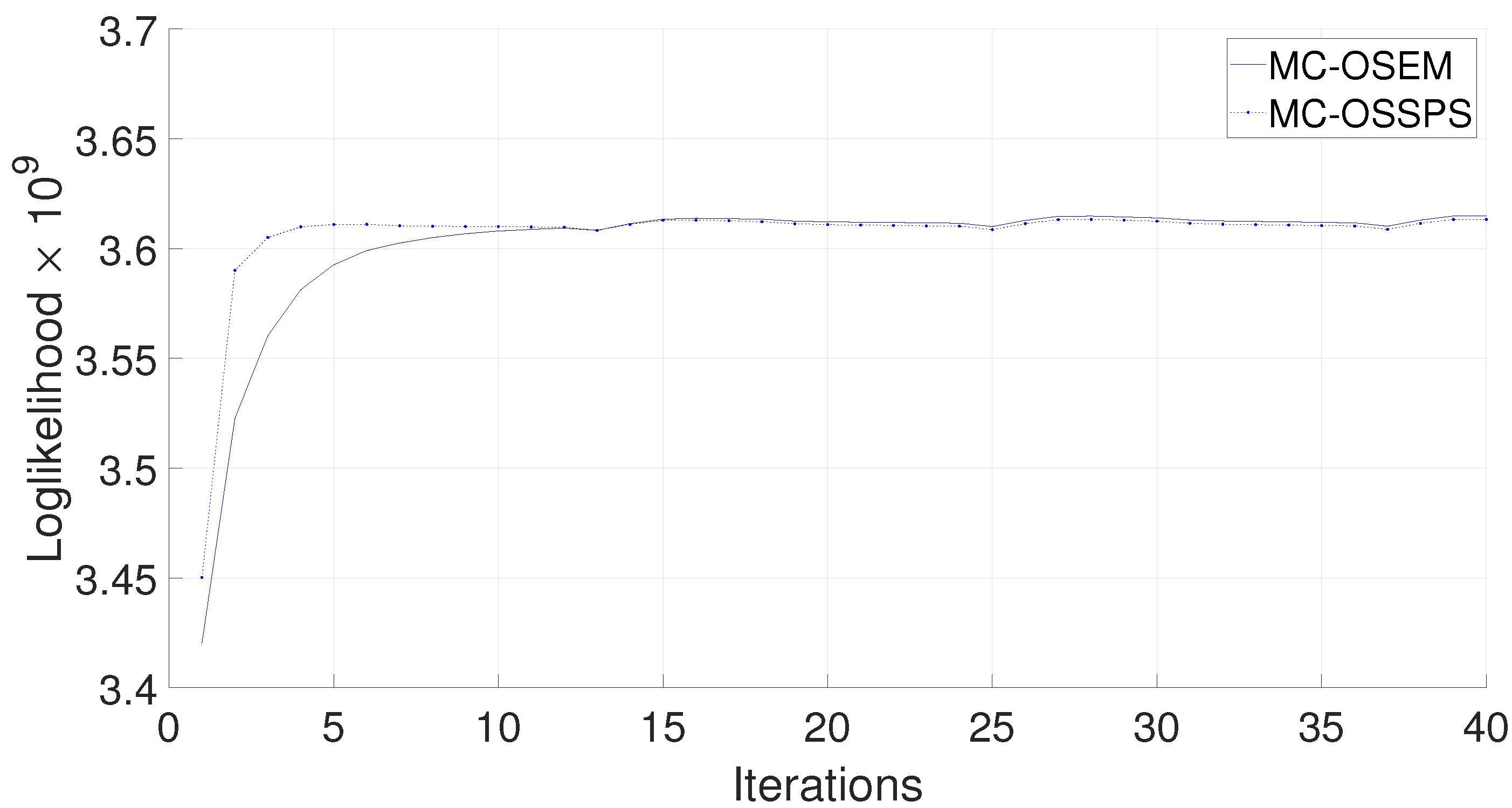
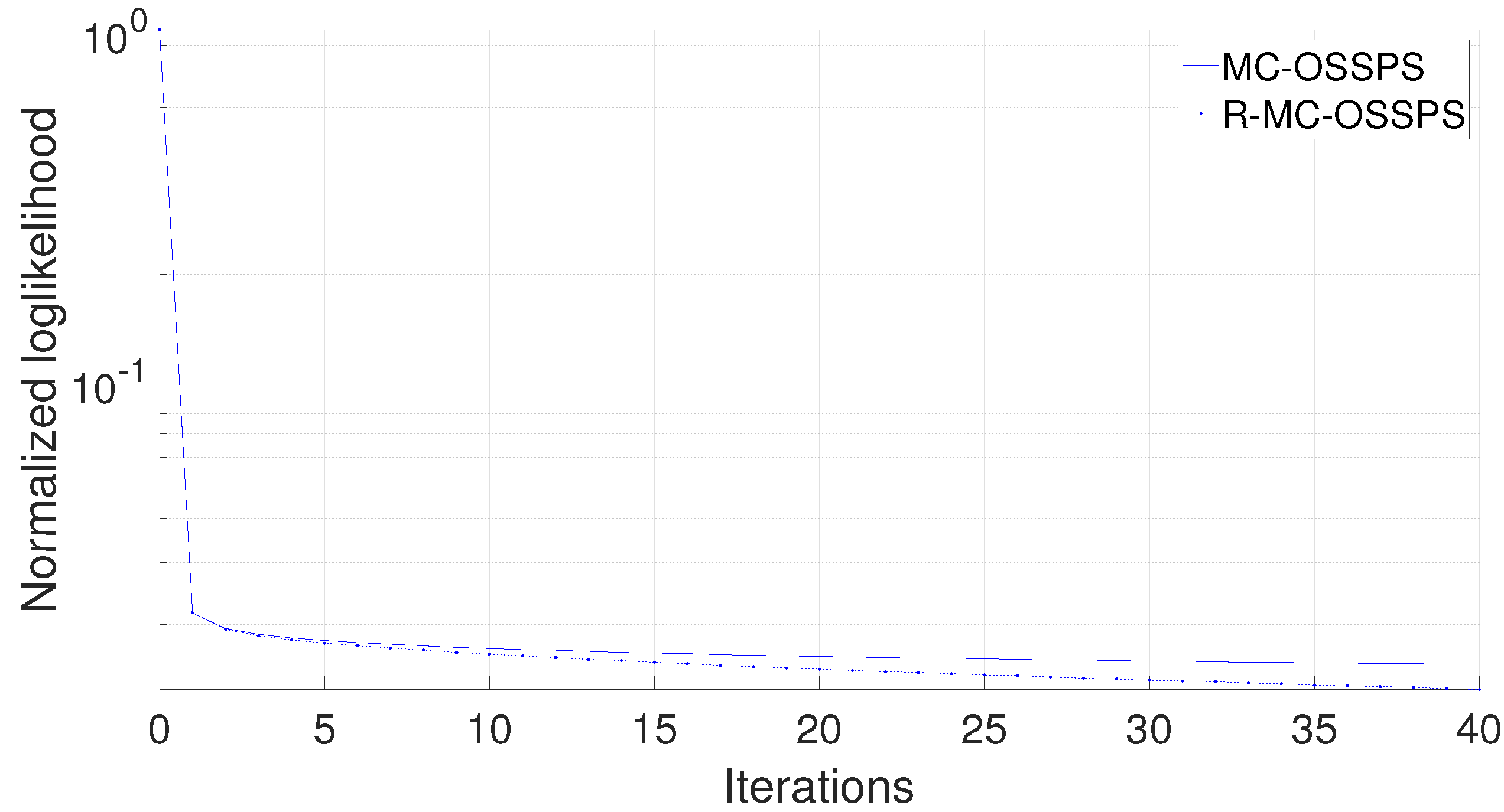
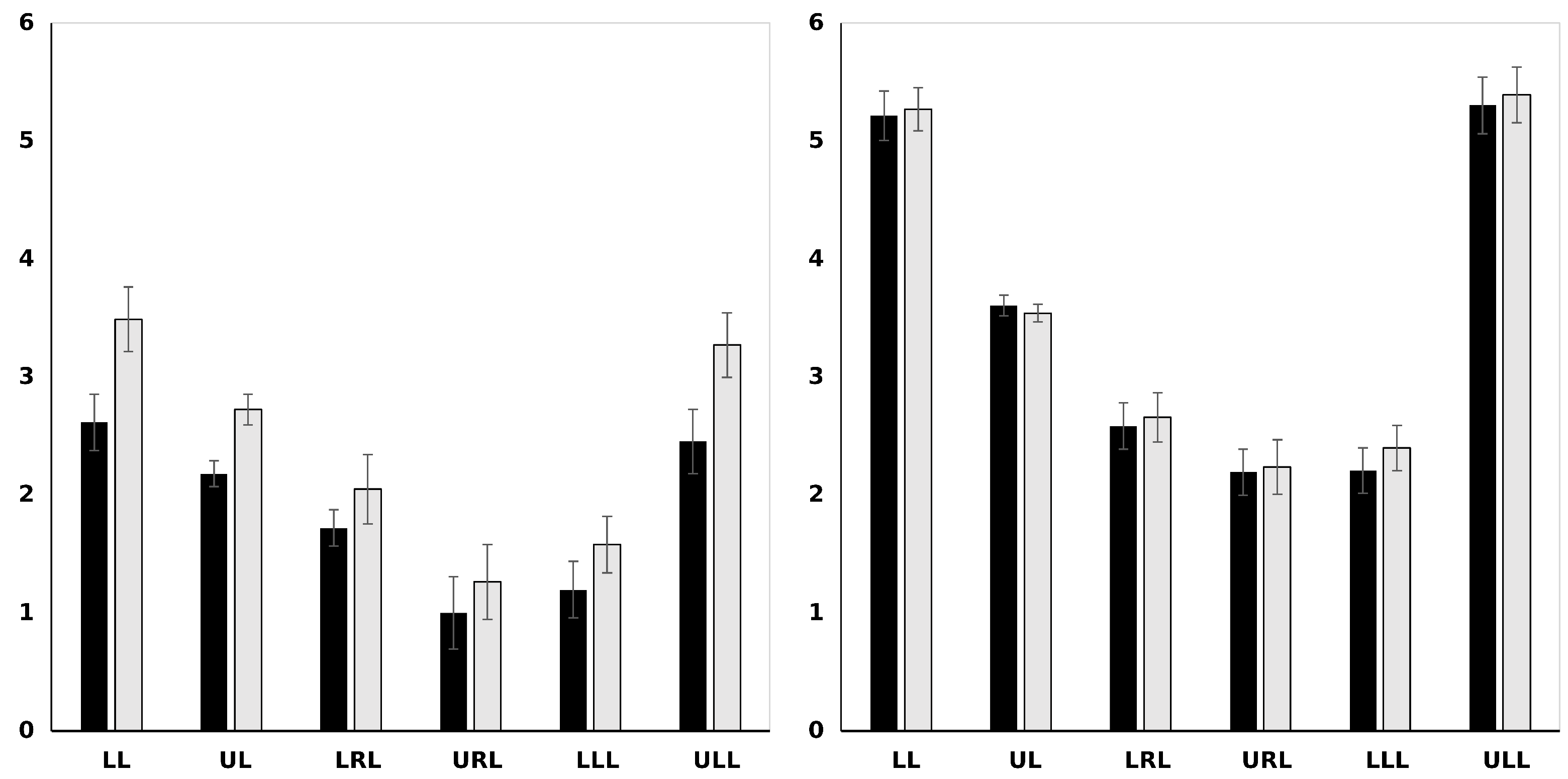
6.2. Comparison of MC-OSSPS and R-MC-OSSPS

As presented in Figure 3, the MC-OSSPS algorithm reached a limit cycle at a low iteration number. Figure 4 demonstrates the fact that R-MC-OSSPS converged to a better solution than MC-OSSPS; the ML solution ( λ M L ) used to calculate the normalized loglikelihood was found for the MC-EM algorithm after 200 iterations.
Figure 5 shows images produced from the same noisy data set by MC-OSSPS and R-MC-OSSPS, respectively. The image reconstructed via R-MC-OSSPS has a lower noise level; however, this advantage is lost following post-smoothing, as in Figure 6. MC-OSSPS and R-MC-OSSPS were also compared in terms of lesion percentage bias (see Figure 7) and CNR (see Figure 8). Without post-smoothing, MC-OSSPS had a marginally superior percentage bias; however, R-MC-OSSPS had higher CNR. These differences were reduced with post-smoothing.

7. Discussion

Motion-compensated SPS was shown to accelerate convergence compared to motion-compensated EM, without reaching a limit cycle, as illustrated in Figure 2. Nonetheless, with the incorporation of ordered subsets in the reconstruction setting, the motion-compensated SPS and EM algorithms produced similar convergence rates (Figure 3). Furthermore, both MC-OSEM and MC-OSSPS algorithms depicted in Figure 3 reached a limit cycle at early iterations.
The introduction of relaxation parameters, i.e., diminishing step size, led to a solution closer to the ML solution calculated from the MC-EM algorithm, as shown in Figure 4. R-MC-OSSPS is expected to converge slower than MC-OSSPS due to the relaxation parameters. This leads to lower noise levels for the same number of iterations. This fact is clearly illustrated in Figure 5, explaining the noticeable improvement in CNR (demonstrated in Figure 8) for images without post-smoothing. The CNR advantage of R-MC-OSSPS over MC-OSSPS was eliminated with the application of post-smoothing, resulting in CNR values comparable to the corresponding ones of MC-OSEM. Finally, both MC-OSSPS and R-MC-OSSPS demonstrated positive percentage bias for some of the lesions, as in Figure 7. This is probably due to super-resolution, provided that the sampling of the underlying distribution of multi-gate data is improved, as in [51].

8. Conclusions

Employing SPS likelihood functions instead of the loglikelihood functions usually adopted in expectation maximization algorithms was proven to be beneficial compared to the classic MC-EM and MC-OSEM. Our study concentrated on the improvement of motion correction algorithms, both in terms of image quality and computational cost, by introducing, for the first time, the separable parabolic surrogate functions framework. The theoretical basis of our novel SPS-based motion correction algorithm lies within the fact that its loglikelihood is upper bounded by the standard EM loglikelihood, thus it will converge faster than EM. This is of particular importance in PET motion correction, where reconstructions are very computationally demanding. In future studies, we intend to include the clinical translation of our proposed reconstruction methods, aiming to improve motion-compensation PET image reconstruction.

Author Contributions

Conceptualization, N.E.P. and N.D.; methodology, N.E.P., G.A.K. and N.D.; software and validation, N.E.P., G.A.K., A.D.F., A.G.T., D.V. and N.D.; writing—original draft preparation, N.E.P.; writing—review and editing, N.E.P., G.A.K., A.D.F., A.G.T., D.V. and N.D.; visualization, N.E.P., G.A.K. and N.D.; supervision, N.D. All authors have read and agreed to the published version of the manuscript.

Funding

This research was partially supported by the research programme No. 200/977 of the Research Committee of the Academy of Athens. Furthermore, this work has been co-financed by the European Union and Greek national funds through the Operational Program Competitiveness, Entrepreneurship and Innovation, under the call RESEARCH-CREATE-INNOVATE (project code: TAEDK-06189).

Institutional Review Board Statement

Not applicable.

Informed Consent Statement

Not applicable.

Data Availability Statement

The data presented in this study are available on request from the corresponding author.

Conflicts of Interest

The authors declare no conflict of interest.

References

  1. Sommer, K.; Saalbach, A.; Brosch, T.; Hall, C.; Cross, N.; Andre, J. Correction of motion artifacts using a multiscale fully convolutional neural network. Am. J. Neuroradiol. 2020, 41, 416–423. [Google Scholar] [CrossRef] [PubMed]
  2. Papathanassiou, D.; Becker, S.; Amir, R.; Menéroux, B.; Liehn, J.C. Respiratory motion artefact in the liver dome on FDG PET/CT: Comparison of attenuation correction with CT and a caesium external source. Eur. J. Nucl. Med. Mol. Imaging 2005, 32, 1422–1428. [Google Scholar] [CrossRef] [PubMed]
  3. Vandenberghe, S.; Moskal, P.; Karp, J.S. State of the art in total body PET. EJNMMI Phys. 2020, 7, 1–33. [Google Scholar] [CrossRef] [PubMed]
  4. Manjeshwar, R.; Tao, X.; Asma, E.; Thielemans, K. Motion compensated image reconstruction of respiratory gated PET/CT. In Proceedings of the 3rd IEEE International Symposium on Biomedical Imaging: Nano to Macro, Arlington, VA, USA, 6–9 April 2006; pp. 674–677. [Google Scholar] [CrossRef]
  5. Kyme, A.Z.; Fulton, R.R. Motion estimation and correction in SPECT, PET and CT. Phys. Med. Biol. 2021, 66, 18TR02. [Google Scholar] [CrossRef]
  6. Chen, S.; Fraum, T.J.; Eldeniz, C.; Mhlanga, J.; Gan, W.; Vahle, T.; Krishnamurthy, U.B.; Faul, D.; Gach, H.M.; Binkley, M.M.; et al. MR-assisted PET respiratory motion correction using deep-learning based short-scan motion fields. Magn. Reson. Med. 2022, 88, 676–690. [Google Scholar] [CrossRef]
  7. Sun, T.; Wu, Y.; Wei, W.; Fu, F.; Meng, N.; Chen, H.; Li, X.; Bai, Y.; Wang, Z.; Ding, J.; et al. Motion correction and its impact on quantification in dynamic total-body 18F-Fluorodeoxyglucose PET. EJNMMI Phys. 2022, 9, 1–16. [Google Scholar] [CrossRef]
  8. Nehmeh, S.A.; Erdi, Y.E.; Ling, C.C.; Rosenzweig, K.E.; Schoder, H.; Larson, S.M.; Macapinlac, H.A.; Squire, O.D.; Humm, J.L. Effect of respiratory gating on quantifying PET images of lung cancer. J. Nucl. Med. 2002, 43, 876–881. [Google Scholar]
  9. Thielemans, K.; Mustafovic, S.; Schnorr, L. Image reconstruction of motion corrected sinograms. In Proceedings of the 2003 IEEE Nuclear Science Symposium. Conference Record (IEEE Cat. No.03CH37515), Portland, OR, USA, 19–25 October 2003; Volume 4, pp. 2401–2406. [Google Scholar] [CrossRef]
  10. Zhou, V.; Kyme, A.; Meikle, S.R.; Fulton, R. Reducing event losses in sinogram-based PET motion correction by extending the axial field of view. In Proceedings of the 2013 IEEE Nuclear Science Symposium and Medical Imaging Conference (2013 NSS/MIC), Seoul, Republic of Korea, 27 October–2 November 2013; pp. 1–4. [Google Scholar] [CrossRef]
  11. Rahmin, A. Advanced motion correction methods in PET. Iran. J. Nucl. Med. 2005, 13, 24–33. [Google Scholar]
  12. Dikaios, N.; Fryer, T.D. Registration-weighted motion correction for PET. Med. Phys. 2012, 39, 1253–1264. [Google Scholar] [CrossRef]
  13. Dikaios, N.; Fryer, T.D. Improved motion-compensated image reconstruction for PET using sensitivity correction per respiratory gate and an approximate tube-of-response backprojector. Med. Phys. 2011, 38, 4958–4970. [Google Scholar] [CrossRef]
  14. Picard, Y.; Thompson, C.J. Motion correction of PET images using multiple acquisition frames. IEEE Trans. Med. Imaging 1997, 16, 137–144. [Google Scholar] [CrossRef] [PubMed] [Green Version]
  15. Dawood, M.; Lang, N.; Jiang, X.; Schafers, K.P. Lung motion correction on respiratory gated 3-D PET/CT images. IEEE Trans. Med. Imaging 2006, 25, 476–485. [Google Scholar] [CrossRef] [PubMed]
  16. Dawood, M.; Buther, F.; Jiang, X.; Schafers, K.P. Respiratory motion correction in 3-D PET data with advanced optical flow algorithms. IEEE Trans. Med. Imaging 2008, 27, 1164–1175. [Google Scholar] [CrossRef] [PubMed]
  17. Bai, W.; Brady, M. Regularized B-spline deformable registration for respiratory motion correction in PET images. Phys. Med. Biol. 2009, 54, 2719. [Google Scholar] [CrossRef] [PubMed]
  18. Jacobson, M.; Fessler, J. Joint estimation of image and deformation parameters in motion-corrected PET. In Proceedings of the 2003 IEEE Nuclear Science Symposium. Conference Record (IEEE Cat. No.03CH37515), Portland, OR, USA, 19–25 October 2003; Volume 5, pp. 3290–3294. [Google Scholar] [CrossRef] [Green Version]
  19. Li, T.; Thorndyke, B.; Schreibmann, E.; Yang, Y.; Xing, L. Model-based image reconstruction for four-dimensional PET. Med. Phys. 2006, 33, 1288–1298. [Google Scholar] [CrossRef] [PubMed]
  20. Qiao, F.; Pan, T.; Clark, J.W.; Mawlawi, O.R. A motion-incorporated reconstruction method for gated PET studies. Phys. Med. Biol. 2006, 51, 3769. [Google Scholar] [CrossRef]
  21. Thielemans, K.; Manjeshwar, R.M.; Tao, X.; Asma, E. Lesion detectability in motion compensated image reconstruction of respiratory gated PET/CT. In Proceedings of the 2006 IEEE Nuclear Science Symposium Conference Record, San Diego, CA, USA, 29 October–1 November 2006; Volume 6, pp. 3278–3282. [Google Scholar] [CrossRef]
  22. Lamare, F.; Carbayo, M.L.; Cresson, T.; Kontaxakis, G.; Santos, A.; Le Rest, C.C.; Reader, A.; Visvikis, D. List-mode-based reconstruction for respiratory motion correction in PET using non-rigid body transformations. Phys. Med. Biol. 2007, 52, 5187. [Google Scholar] [CrossRef]
  23. Reyes, M.; Malandain, G.; Koulibaly, P.M.; González-Ballester, M.A.; Darcourt, J. Model-based respiratory motion compensation for emission tomography image reconstruction. Phys. Med. Biol. 2007, 52, 3579. [Google Scholar] [CrossRef] [Green Version]
  24. Dikaios, N.; Fryer, T. Acceleration of motion-compensated PET reconstruction: Ordered subsets-gates EM algorithms and a priori reference gate information. Phys. Med. Biol. 2011, 56, 1695. [Google Scholar] [CrossRef]
  25. Polycarpou, I.; Soultanidis, G.; Tsoumpas, C. Synergistic motion compensation strategies for positron emission tomography when acquired simultaneously with magnetic resonance imaging. Philos. Trans. R. Soc. 2021, 379, 20200207. [Google Scholar] [CrossRef]
  26. Guérin, B.; Cho, S.; Chun, S.Y.; Zhu, X.; Alpert, N.; El Fakhri, G.; Reese, T.; Catana, C. Nonrigid PET motion compensation in the lower abdomen using simultaneous tagged-MRI and PET imaging. Med. Phys. 2011, 38, 3025–3038. [Google Scholar] [CrossRef] [PubMed]
  27. Manber, R.; Thielemans, K.; Hutton, B.F.; Barnes, A.; Ourselin, S.; Arridge, S.; O’Meara, C.; Wan, S.; Atkinson, D. Practical PET respiratory motion correction in clinical PET/MR. J. Nucl. Med. 2015, 56, 890–896. [Google Scholar] [CrossRef] [PubMed] [Green Version]
  28. Ippoliti, M.; Lukas, M.; Brenner, W.; Schatka, I.; Furth, C.; Schaeffter, T.; Makowski, M.R.; Kolbitsch, C. Respiratory motion correction for enhanced quantification of hepatic lesions in simultaneous PET and DCE-MR imaging. Phys. Med. Biol. 2021, 66, 095012. [Google Scholar] [CrossRef] [PubMed]
  29. Petibon, Y.; Huang, C.; Ouyang, J.; Reese, T.G.; Li, Q.; Syrkina, A.; Chen, Y.L.; El Fakhri, G. Relative role of motion and PSF compensation in whole-body oncologic PET-MR imaging. Med. Phys. 2014, 41, 042503. [Google Scholar] [CrossRef] [Green Version]
  30. Huang, C.; Ackerman, J.L.; Petibon, Y.; Normandin, M.D.; Brady, T.J.; El Fakhri, G.; Ouyang, J. Motion compensation for brain PET imaging using wireless MR active markers in simultaneous PET–MR: Phantom and non-human primate studies. NeuroImage 2014, 91, 129–137. [Google Scholar] [CrossRef] [Green Version]
  31. Guo, X.; Zhou, B.; Pigg, D.; Spottiswoode, B.; Casey, M.E.; Liu, C.; Dvornek, N.C. Unsupervised inter-frame motion correction for whole-body dynamic PET using convolutional long short-term memory in a convolutional neural network. Med. Image Anal. 2022, 80, 102524. [Google Scholar] [CrossRef] [PubMed]
  32. Zhou, B.; Tsai, Y.J.; Chen, X.; Duncan, J.S.; Liu, C. MDPET: A unified motion correction and denoising adversarial network for low-dose gated PET. IEEE Trans. Med. Imaging 2021, 40, 3154–3164. [Google Scholar] [CrossRef]
  33. Lamare, F.; Bousse, A.; Thielemans, K.; Liu, C.; Merlin, T.; Fayad, H.; Visvikis, D. PET respiratory motion correction: Quo vadis? Phys. Med. Biol. 2022, 67, 03TR02. [Google Scholar] [CrossRef]
  34. Hudson, H.M.; Larkin, R.S. Accelerated image reconstruction using ordered subsets of projection data. IEEE Trans. Med. Imaging 1994, 13, 601–609. [Google Scholar] [CrossRef] [Green Version]
  35. Green, P.J. Bayesian reconstructions from emission tomography data using a modified EM algorithm. IEEE Trans. Med. Imaging 1990, 9, 84–93. [Google Scholar] [CrossRef] [Green Version]
  36. Fessler, J.A.; Hero, A.O. Penalized maximum-likelihood image reconstruction using space-alternating generalized EM algorithms. IEEE Trans. Med. Imaging 1995, 4, 1417–1429. [Google Scholar] [CrossRef] [PubMed]
  37. Fessler, J.; Erdogan, H. A paraboloidal surrogates algorithm for convergent penalized-likelihood emission image reconstruction. In Proceedings of the 1998 IEEE Nuclear Science Symposium Conference Record. 1998 IEEE Nuclear Science Symposium and Medical Imaging Conference (Cat. No.98CH36255), Toronto, ON, Canada, 8–14 November 1998; Volume 2, pp. 1132–1135. [Google Scholar] [CrossRef] [Green Version]
  38. Dikaios, N. Respiratory Motion Correction for Positron Emission Tomography. Ph.D. Thesis, Wolfson College, University of Cambridge, Cambridge, UK, 2011. [Google Scholar]
  39. Dempster, A.P.; Laird, N.M.; Rubin, D.B. Maximum likelihood from incomplete data via the EM algorithm. J. R. Stat. Soc. Ser. B Methodol. 1977, 39, 1–22. [Google Scholar] [CrossRef]
  40. Shepp, L.A.; Vardi, Y. Maximum likelihood reconstruction for emission tomography. IEEE Trans. Med. Imaging 1982, 1, 113–122. [Google Scholar] [CrossRef]
  41. Lange, K.; Carson, R. EM reconstruction algorithms for emission and transmission tomography. J. Comput. Assist. Tomogr. 1984, 8, 306–316. [Google Scholar] [PubMed]
  42. Moskal, P.; Zoń, N.; Bednarski, T.; Białas, P.; Czerwiński, E.; Gajos, A.; Kamińska, D.; Kochanowski, A.; Korcyl, G.; Kowal, J.; et al. A novel method for the line-of-response and time-of-flight reconstruction in TOF-PET detectors based on a library of synchronized model signals. Nucl. Instrum. Methods. Phys. Res. B 2015, 775, 54–62. [Google Scholar] [CrossRef] [Green Version]
  43. Lin, H.; Guo, X.; Jing, J.; Mao, X.; Yang, Y.; Hu, M. An automatic method to generate voxel-based absorbed doses from radioactivity distributions for nuclear medicine using generative adversarial networks: A feasibility study. Phys. Eng. Sci. Med. 2022, 45, 971–980. [Google Scholar] [CrossRef]
  44. Browne, J.; De Pierro, A. A row-action alternative to the EM algorithm for maximizing likelihood in emission tomography. IEEE Trans. Med. Imaging 1996, 15, 687–699. [Google Scholar] [CrossRef]
  45. Erdogan, H.; Fessler, J. Monotonic algorithms for transmission tomography. In Proceedings of the 5th IEEE EMBS International Summer School on Biomedical Imaging, Berder Island, France, 15–23 June 2002; p. 14. [Google Scholar] [CrossRef] [Green Version]
  46. Erdogan, H.; Fessler, J.A. Ordered subsets algorithms for transmission tomography. Phys. Med. Biol. 1999, 44, 2835. [Google Scholar] [CrossRef]
  47. Ahn, S.; Fessler, J.A. Globally convergent image reconstruction for emission tomography using relaxed ordered subsets algorithms. IEEE Trans. Med. Imaging 2003, 22, 613–626. [Google Scholar] [CrossRef] [Green Version]
  48. Segars, W.P.; Lalush, D.S.; Tsui, B.M. Modeling respiratory mechanics in the MCAT and spline-based MCAT phantoms. IEEE Trans. Med. Imaging 2001, 48, 89–97. [Google Scholar] [CrossRef]
  49. Ibanez, L.; Schroeder, W.; Ng, L.; Cates, J. The ITK Software Guide: The Insight Segmentation and Registration Toolkit; Kitware, Inc.: New York, NY, USA, 2005. [Google Scholar]
  50. Thielemans, K.; Tsoumpas, C.; Mustafovic, S.; Beisel, T.; Aguiar, P.; Dikaios, N.; Jacobson, M.W. STIR: Software for tomographic image reconstruction release 2. Phys. Med. Biol. 2012, 57, 867. [Google Scholar] [CrossRef] [PubMed] [Green Version]
  51. Kennedy, J.A.; Israel, O.; Frenkel, A.; Bar-Shalom, R.; Azhari, H. Super-resolution in PET imaging. IEEE Trans. Med. Imaging 2006, 25, 137–147. [Google Scholar] [CrossRef] [PubMed]
Figure 1. Loglikelihood, L b ( y b | λ n ) , and the parabolic surrogate function, ϕ b ( y ¯ b | y ¯ b n ) .
Mathematics 11 00055 g001
Figure 2. Loglikelihood vs. iteration number for MC-EM and MC-SPS.
Mathematics 11 00055 g002
Figure 3. Loglikelihood vs. iteration number for MC-OSEM and MC-OSSPS. In both cases 12 subsets were employed.
Mathematics 11 00055 g003
Figure 4. Normalized loglikelihood L ( y | λ L M ) L ( y | λ n ) L ( y | λ L M ) L ( y | λ 0 ) vs. iteration number for R-MC-OSSPS and MC-OSSPS. Note that the y-axis is in logarithmic scale.
Mathematics 11 00055 g004
Figure 5. Transverse, coronal, and sagittal planes for PET images of the NCAT phantom reconstructed from noisy data with MC-OSSPS (top row) and R-MC-OSSPS (bottom row). Both images used 40 iterations with 12 subsets. Post-smoothing was not applied. The linear greyscale is thresholded at a standardized uptake value (SUV) equal to 6.
Mathematics 11 00055 g005
Figure 6. Post-smoothed images (6 mm FWHM Gaussian) of the NCAT phantom, resulting from the reconstructions in Figure 5.
Mathematics 11 00055 g006
Figure 7. Lesion percentage bias for the six lesions for MC-OSSPS and R-MC-OSSPS. Left: without post-smoothing; right: with 6 mm Gaussian post-smoothing. Solid and hollow bars show the mean values for noisy data (10 noise realizations) with MC-OSSPS and R-MC-OSSPS, respectively. The error bars denote the standard deviation of the percentage bias values over the 10 noise realizations. The lesions are lower liver (LL), upper liver (UL), lower right lung (LRL), upper right lung (URL), lower left lung (LLL), and upper left lung (ULL).
Mathematics 11 00055 g007
Figure 8. Lesion contrast-to-noise ratio (CNR) for the six lesions for MC-OSSPS and R-MC-OSSPS. Left: without post-smoothing; right: with 6 mm Gaussian post-smoothing. Solid and hollow bars show the mean values for noisy data (10 noise realizations) of MC-OSSPS and R-MC-OSSPS, respectively. The error bars denote the standard deviation of the percentage bias values over the 10 noise realizations. The lesions are lower liver (LL), upper liver (UL), lower right lung (LRL), upper right lung (URL), lower left lung (LLL), and upper left lung (ULL).
Mathematics 11 00055 g008
Disclaimer/Publisher’s Note: The statements, opinions and data contained in all publications are solely those of the individual author(s) and contributor(s) and not of MDPI and/or the editor(s). MDPI and/or the editor(s) disclaim responsibility for any injury to people or property resulting from any ideas, methods, instructions or products referred to in the content.

