Article

Design of Finite Time Reduced Order H∞ Controller for Linear Discrete Time Systems

1
Industrial Technologies and Services Laboratory, Higher School of Technology, Sidi Mohammed Ben Abdellah University, Fez 30000, Morocco
2
LRDSI Laboratory, Department of Physics, Faculty of Sciences and Technology, Abdelmalek Essaâdi University, Al Hoceima 32000, Morocco
3
Department of Physics, Khalifa University, Abu Dhabi P.O. Box 127788, United Arab Emirates
4
Faculty of Sciences, Ibn Tofail University, Kenitra 14000, Morocco
5
LISAC Laboratory, Department of Physics, Faculty of Sciences Dhar El Mehraz, Sidi Mohammed Ben Abdellah University, Fez 30000, Morocco
6
Department of Mathematics, Khalifa University, Abu Dhabi P.O. Box 127788, United Arab Emirates
*
Authors to whom correspondence should be addressed.
Mathematics 2023, 11(1), 31; https://doi.org/10.3390/math11010031
Submission received: 7 November 2022 / Revised: 9 December 2022 / Accepted: 13 December 2022 / Published: 21 December 2022

Abstract

:
The current article gives a new approach that is efficient for the design of a low-order H∞ controller over a finite time interval. The system under consideration is a linear discrete time system affected by norm bounded disturbances. The proposed method has the advantage that takes into account both robustness aspects and desired closed-loop characteristics, reducing the number of variables in Linear Matrix Inequalities (LMIs). Thus, reduced order H∞ controller parameters are given to guarantee a finite time H∞ bound (FTB-H∞) for a closed-loop system. The method of the finite time stability, that is proven in this paper by the Lyapunov theory, can be applied to a wide range of process models. Numerical examples demonstrating the effectiveness of the results developed are presented at the end of this paper.

1. Introduction

Stability is the most important characteristic to be maintained in theoretical and practical control systems [1,2,3,4,5]. Stabilization using full-state feedback gains is studied by many researchers [6,7,8,9,10] thanks to the closed-loop control, which is the simplest and can be realized in practice. In these design approaches, it is taken into account that all states can be determined by direct measurement. However, in most practical situations, it can be very expensive, if not impossible, to set up suitable sensors to directly measure missing system variables. Therefore, the state variables of a dynamic system are often not all available. This problem has gained high interest in real-world systems, such as fault diagnosis and supervision; for this reason, much research discusses the observer design due to the fact that the state cannot be measured frequently [11,12,13,14]. Then, observer-based fault control approaches have been introduced to provide a state-of-the-art overview on the existing fault diagnosis and prognosis to improve the resiliency of control systems against faults and failures. An active fault control is generally more efficient in dealing with different types of faults; however, a controller’s performance is primarily dependent on its fault detection and isolation unit in providing timely and accurate fault information. Many of these ideal results are obtained thanks to pioneering works [15,16]. In addition, many other works discussed the observer-based controller design using these references. Then, the observer-based fuzzy controller for a class of nonlinear systems is considered in [17,18]. In [19], the novel Lyapunov–Krasovskii functional (LKF) is used to present an observer-based controller design method for linear systems with varying state delays over time intervals. On the other hand, the paper [20] introduces integral-based triggering conditions to design the observer-based controller for linear systems with disturbances. Therefore, a model-based format is used to generate control signals. In daily life, disturbances are very common. In control processes, not only can the reference input influence the output, but the disturbances can also have a negative impact on the output. So in the observer design, disturbances are taken into account by many authors [7,21,22,23]. Moreover, most of the processes are described by state-space systems which can be either nonlinear or linear in form; usually, a real system or process is described by a nonlinear model, whereas in order to estimate and control the system, most mathematical tools are more accessible to a linear model. The results for linearized models are easy to reproduce using the usual numerical tools, as there are clear rules to tune these controllers where an equilibrium point is configured, and then high levels of performance and reliability can be achieved. However, these results treat the observer-based controllers in the full order, in which all cases are estimated. Then, the implementation of this observer in complex systems is difficult, which is unnecessary in many studies when the case’s unavailability is partial. To overcome these weaknesses in such types of systems, the solution is to use a reduced-order observer-based controller in order to compensate for a specific unavailable portion of the system states.
In this sense, new observer-based controllers are developed to ensure a certain level of performance that includes the reduced order H∞ parameters. Then, the problem of the optimal reduced-order filter for linear descriptor systems is considered in [24], where necessary and sufficient conditions are obtained for the existence of unbiased causal filters. In [25], a reduced-order disturbances observer is proposed to reduce the after-effects caused by the friction on the output of the traditional PD-type control scheme, rather than to compensate for the initial friction mechanics. The paper [26] discusses the design of reduced-order observer-based controllers for the stabilization of large discrete-time linear control systems. This design is achieved by deriving a reduced order model for the given linear factory using the dominant state of the linear factory. Additionally, a novel reference compensation technique is presented in [27] to attenuate the after-effects caused by the friction. A linear control law based on a low-order observer has been proposed to realize this strategy. Most of these studies deal with observation systems in an infinite period of time. This means that you can obtain the estimated state, but in some cases you will get a large value, which may not be feasible from a practical point of view, and this is unacceptable. For this reason, the concepts of Finite Time Stability (FTS) and FTB are introduced. On the other hand, it is important to note that FTS and Lyapunov asymptotic stability are two independent concepts; in fact, the system can be FTS but not asymptotically stable, and vice versa.
The FTS and the finite time H∞ control problems attracted great attention from both the academic and industrial communities [28,29,30,31]. The contributions of the paper [10] indicate that the new controller can achieve a finite time convergence, loosen the constraint conditions according to which non-affine functions must be derived and strictly positive or negative, and significantly reduce the load of computation. The study [29] also addresses the finite time tracking control problem for switched nonlinear systems with random switching and hysteresis inputs. The authors in [23] develop a fast convergence output feedback control algorithm based on back-stepping finite time command filtering. On the other hand, the observer-based finite time H∞ control problem is studied in [30,31] for a class of discrete-time Markovian jump systems with time-varying norm-bounded disturbances. In order to simplify the estimation error, the unbiasedness concept is used to reduce the complexity and computational burden of the real time filtering process. The previous results have some limits of applicability for complex systems because of the observer-based model order that is the same as that of the system. Then, we investigate in this paper the FTB-H∞ problem where the observer-based filter is used to estimate the control law and not the state vector, as it is given in the literature. There are not many results related to the reduced order H∞ controller in finite time, especially for discrete linear systems; but for continuous systems, we can find some works [32,33,34,35] dealing with the FTB-H∞ problem where the unbiasedness conditions of the estimation error are explicitly taken into account. Thus, the proposed approach is inspired by the previous results, but the discrete linear systems, which is still an open problem for many types of systems, are discussed here. The various issues addressed in this paper bring our approach closer to reality compared to what has been presented in the literature; therefore, this work is more realistic and represents a major step forward to address many problems. The significance of the proposed approach lies not only in solving the studied problems, but also in reducing the number of variables in LMIs by making all parameters dependent on a single matrix variable. Thus, this strategy is effective to reduce the computational cost of the real process.
When studying a system, modeling is a very necessary step because it defines the methods that will then be used to analyze its properties. Therefore, in order to get closer to the behavior of real processes, better modeling consists in studying the systems taking into account certain information, which previous studies are unable to do. Motivated by these observations, this paper deals with the problems that these types of systems face theoretically before moving on to address them practically. Then, a new form of a robust reduced order H∞ controller is investigated. The purpose is to determine controller parameters in order to guarantee the FTB-H∞ and stability of the closed-loop system. Additionally, the order of the designed controller is the same as the controller input u k . On the other hand, disturbances in the system components are among the main reasons for instability and degraded control performance. Thus, finite time convergence, robustness, systems dynamics and near-zero error are the advantages of the proposed technique. From the algebraic constraints arising from the analysis of the estimation error, a parameterization of the filter matrices is obtained. Based on the parametrization results, the design problem is solved in two steps, and these steps permit the determination of the controller parameters via a solution of an LMI optimization problem. Finally, the less conservative LMI-based design conditions of the controller are proposed and can be solved by the LMI tools of MATLAB. Then, a thorough comparison of several different aspects is conducted to understand the advantages and disadvantages of various techniques to motivate researchers to further develop approaches for designing robust reduced order H∞ controllers.
The paper is organized as follows. The FTB-H∞ problem is formulated in Section 2. In Section 3, some results are derived and given by Theorem 1 to synthesize the FTB-H∞ filter-based controller. Theorem 2 is then presented to solve the design problem. The proposed controller design procedure is presented in Section 4. In Section 5, numerical examples are provided to illustrate the efficiency of the proposed approach. Finally, some conclusions are drawn in Section 6.

2. Preliminaries and Problem Definition

The following notations are used throughout the paper: n is the n dimensional Euclidean space; r a n k Υ is the rank of matrix Υ ; λ m i n P and λ m a x P are the minimum and maximum eigenvalues, respectively, of the matrix P ; I and 0 are, respectively, the identity and zero matrices of appropriate dimensions; 1 is the inverse of a matrix; is the symmetric block in a matrix; and the superscript T is the matrix transposition. Then, consider the following linear time-invariant system:
x k + 1 = A x k + B u k + D x w k z k     = C z x k + D z w k y k     = C y x k + D y w k
where x k n is the state space vector, u k m   m n is the control input vector, z k q is the controller output, and y k p is the measured output. Additionally, w k r is the disturbances vector of finite energy which belongs to the following set:
W = w k ,   k 0 , N   : k = 0 N w T k w k < d 2
Now, we recall an assumption and some definitions on the FTS and the FTB.
Assumption 1. 
A , B and A , C y are controllable and observable.
Definition 1 
[24,36]. The linear system
x k + 1 = A x k ,       x 0 = x 0  
is said to be FTS with respect to c 1 , c 2 , N , R , where   c 2 > c 1 > 0   and   R > 0 , if
x T 0 R x 0 < c 1 2     x T k R x k < c 2 2 ,       k 1 , N
Definition 2 
[37,38]. The linear system
x k + 1 = A x k + D x w k ,       x 0 = x 0
is said to be FTB with respect to c 1 , c 2 , d , N , R , where   c 2 > c 1 > 0   and   R > 0 , if
x T 0 R x 0 < c 1 2     x T k R x k < c 2 2 ,     k 1 , N
Definition 3 
[38]. The linear system
x k + 1 = A x k + D x w k ,       x 0 = x 0 z k       = C z x k + D z w k
is said to be FTB-H∞, with respect to c 1 , c 2 , d , N , R , γ , if there is a FTB with respect to c 1 , c 2 , d , N , R  and under the zero-initial condition. Then, the output z k satisfies:
k = 0 N z T k z k γ 2 k = 0 N w T k w k
Lemma 1. 
The system (7) is said to be FTB-H∞, with respect to 0 , c 2 , d , N , R , γ , if there exist a scalar α 1 and a symmetric positive definite matrix P such that:
α P ˜ 0 A T P ˜ C z T γ 2 α N I D x T P ˜ D z T P ˜ 0 I < 0 ,
γ 2 d 2 < λ m i n P c 2 2
where P ˜ = R 1 2 P R 1 2 .
Proof. 
The proof of this lemma can be completed in the same way as described in the papers [32,33,34]. □
Remark 1. 
It is important to note that the FTB of the estimation error means that the dynamic output generated by the controller does not necessarily converge to the static output at a specific time, and then the difference between them does not cause any problem. Thus, this difference does not exceed certain limits for a finite interval of time. On the other hand, the FTS concept of the estimation error can bring us back to a new concept called finite time estimation. Then, the dynamic output u k of the functional filter is said to be finite time H∞ estimation (FTE-H∞) of the static output if the estimation error is FTB-H∞.
Remark 2. 
There are reduced order H∞ controllers in finite time that are designed for continuous systems in [32,33,34,35]. Then, there is no continuity of works to design controllers for discrete linear systems that are near to the process in real life. Thus, due to the difficulty of designing controllers in this type of system, we do not find much research on this subject despite its importance, so we decided to dive into this subject.

3. Main Results

3.1. FTB-H∞ Filter-Based Controller Synthesis

Based on Lemma 1, some results are now derived using the control law u k = K u x k . Then, the system (1) can be rewritten as follows:
x k + 1 = A + B K u x k + D x w k z k     = C z x k + D z w k
Theorem 1. 
The system (11) is said to be FTB-H∞, with respect to 0 , c 2 , d , N , R , γ , if there exists a scalar α 1 , a symmetric positive definite matrix X , and an appropriately sized matrix Y such that ( X ˜ = R 1 2 X R 1 2 ); the conditions
α X 0 X A T + Y T B T X C z T γ 2 α N I D x T D z T X 0 I < 0 ,
λ m a x X ˜ γ 2 d 2 < c 2 2
are satisfied where the feedback controller is K u = Y X 1 .
Proof. 
Pre- and post-multiplying the matrix (9) by d i a g P ˜ 1 , I , P ˜ 1 , I , we have:
α P ˜ 1 0 P ˜ 1 A T P ˜ 1 C z T γ 2 α N I D x T D z T P ˜ 1 0 I < 0
Then, replacing the matrix A by A + B K u and choosing X = P ˜ 1 , Y = K u X , the result of Theorem 1 is obtained.
Now consider the FTB-H∞ functional filter-based controller of the form
x ^ k + 1 = A f x ^ k + L f y k + G u k u k   = x ^ k + K y k
where   x ^ k m is the controller state, which has the same dimension as the control input. A f , L f , G , and K are matrices of appropriate dimensions that will be determined. Then it is clear that the order of the observer-based controller is reduced since dim x ^ k = m n . □
Remark 3. 
The objective of this paper is to determine the matrices A f , L f , G ,   and   K of the proposed filter such that:
  • The filter is unbiased: the error  e k   does not depend explicitly on  x k   and   u k   if  w k = 0 ;
  • The effect of disturbances on controlled output is minimized if w k 0 ;
  • The FTB-H∞ of the closed-loop system is guaranteed.
Remark 4. 
From Theorem 1, the state feedback gain K u is obtained by seeking the matrix (12), so the system (11) is FTB-H∞ with respect to 0 , c 2 , d , N , R , γ . In the following, to use the functional filter-based controller (14) and estimate the control law u k = K u x k , we assume that the whole space is not measurable. This paper proposes a standard reduced Kalman filter that takes into account the unbiasedness of the estimation error [39].
Then, the estimation error is given by:
e k = K u x k u k = K u x k x ^ k K y k = K u x k x ^ k K C y x k + D y w k
Thus, we obtain:
e k = ψ x k x ^ k K D y w k
where
ψ = K u K C y
Letting   ε k = ψ x k x ^ k , the Equation (15) can be rewritten as
ε k = ψ x k x ^ k   e k = ε k K D y w k
Considering (1) and (14), we have:
ε k + 1 = A f ε k + ψ A A f ψ L f C y x k + ψ B G u k + ψ D x L f D y w k
From the paper [24], the necessary and sufficient condition for filter unbiasedness is given by
ψ A A f ψ L f C y = 0
ψ B G = 0
Using (1), (16), (17), and (14), we have:
x k + 1 = A x k + B u k + D x w k = A x k + B x ^ k + K y k + D x w k = A x k + B ψ x k ε k + B K C y x k + D y w k + D x w k = A + B K u x k B ε k + B K D y + D x w k
Under the unbiasedness conditions, we can rewrite the Equations (18) and (21) as follows:
x k + 1 = A + B K u x k B ε k + B K D y + D x w k ε k + 1 = A f ε k + ψ D x L f D y w k   e k     = ε k K D y w k
On the other hand, we obtain the following equation using (16) in (19):
K u A K C y A A f K u + A f K L f C y = 0
and so
A f K u + J C y + K C y A = K u A
where
J = L f A f K
Equation (23) can be rewritten as
Χ Υ = Λ
where
Χ = A f J K
Υ = K u C y C y A
Λ = K u A
Thus, the Equation (25) has a solution if and only if
r a n k Υ Λ = r a n k Υ
The general solution of (25) has the form (30) where Υ +   is the generalized inverse of matrix   Υ i.e. ,   Υ = Υ Υ + Υ   and   Ζ   is an arbitrary matrix with appropriate dimension.
Χ = Λ Υ + + Ζ I Υ Υ +
Using (26)–(28), and (30), we obtain:
A f = Χ I 0 0 = E 11 + Z F 11
J = Χ 0 I 0 = E 22 + Z F 22
K = Χ 0 0 I = E 33 + Z F 33
where
E 11 = Λ Υ + I 0 0
F 11 = I Υ Υ + I 0 0
E 22 = Λ Υ + 0 I 0
F 22 = I Υ Υ + 0 I 0
  E 33 = Λ Υ + 0 0 I
F 33 = I Υ Υ + 0 0 I
Thus, we can write the following equation using (24), (31)–(33):
L f D y = J + A f K D y = E 22 + Z F 22 + E 11 + Z F 11 E 33 + Z F 33 D y
To overcome the bilinearity problem, due to the product   Z F 11 Z F 33   in the Equation (40), we can choose one of the following conditions:
Z F 33 D y = 0
Z F 33 = 0  
  Z F 11 = 0
Then, the solution of each equation is given by:
Z = Z 1 I F 33 D y F 33 D y +
Z = Z 2 I F 33 F 33 +
Z = Z 4 I F 11 F 11 +
These solutions ((44)–(46)) can have the form:
Z = Z ¯ I V V +
Thus, the matrices   A f ,  J , and   K   are obtained by:
A f = E 11 + Z ¯ F ¯ 11
J = E 22 + Z ¯ F ¯ 22
K = E 33 + Z ¯ F ¯ 33
where
F ¯ 11 = I V V + F 11
F ¯ 22 = I V V + F 22
F ¯ 33 = I V V + F 33
Remark 5. 
The matrices (48)–(50) are obtained using the Equation (47), where the conditions Z F 33 D y , Z F 33 , and Z F 11 are set to zero, to simplify the numerical solution: although this makes the solution only slightly more conservative, it significantly reduces the computational cost.
Remark 6. 
The Equation (40) can take two forms:
  • If we choose the condition (41), the Equation (40) becomes:
    L f D y = E 22 + Z F 22 + E 11 + Z F 11 E 33 D y
  • Now, either we use the condition (42) or the condition (43). Choosing the last condition, the Equation (40) becomes:
    L f D y = E 22 + Z F 22 + E 11 E 33 + Z F 33 D y
Then, in order to make the extraction of the variable   Z   simple, we decided to use the Equation (54) in the future proofs.
Taking into account of (41) or (42), the system (22) becomes as follows:
x k + 1 = A + B K u x k B ε k + B E 33 D y + D x w k ε k + 1 = A f ε k + F ¯ ε w k           e k     = ε k E 33 D y w k
where
F ¯ ε = F ¯ ε 1 Z ¯ F ¯ ε 2
and
F ¯ ε 1 = K u E 33 C y D x E 22 + E 11 E 33 D y
F ¯ ε 2 = F ¯ 33 C y D x + F ¯ 22 + F ¯ 11 E 33 D y
Remark 7. 
New sufficient conditions involving LMIs, which could be solved by employing Matlab LMI toolbox, are established to deal with the FTB-H∞ problem and minimize the effect of disturbances. These conditions are dependent on the parametrization results of algebraic constraints obtained from the unbiasedness conditions of the estimation error.

3.2. LMI Synthesis Conditions

Now, sufficient conditions involving LMIs are given in this paper by Theorem 2 to deal with the FTB-H∞ problem.
Theorem 2. 
The system (56) is said to be FTB-H∞, with respect to 0 , c 2 , d , N , R , γ , if there exist a scalar α 1 , symmetric positive definite matrices P , Q , and an appropriately sized matrix Y such that:
α P ˜ 0 0 A + B K u T P ˜ 0 0 Q 0 B T P ˜ E 11 T Q + F ¯ 11 T Y T I γ 2 α N I B E 33 D y + D x T P ˜ F ¯ ε 1 T Q F ¯ ε 2 T Y T D y T E 33 T P ˜ 0 0 Q 0 I < 0 ,  
d 2 γ 2 < λ m i n P c 2 2
where P ˜ = R 1 2 P R 1 2 .
Proof. 
Consider the following LKF:
V x k = x T k P ˜ x k + ε T k Q ε k
From the LKF (62), we obtain:
V x k + 1 V x k = ξ T k Ω ξ k
where
ξ k = x T k ε T k w T k T
and
Ω = A + B K u T P ˜ A + B K u P ˜ A + B K u T P ˜ B A + B K u T P ˜ B E 33 D y + D x B T P ˜ B + A f T Q A f Q B T P ˜ B E 33 D y + D x + A f T Q F ¯ ε B E 33 D y + D x T P ˜ B E 33 D y + D x + F ¯ ε T Q F ¯ ε
Using the system (56), we have:
e T k e k = ε k w k T I E 33 D y D y T E 33 T E 33 D y ε k w k
Then, it is easy to see that:
V x k + 1 V x k = ξ T k Π ξ k + ξ T k α 1 P ˜ 0 0 0 0 0 0 0 γ 2 α N I ξ k   e T k e k
where
Π = A + B K u T P ˜ A + B K u α P ˜ A + B K u T P ˜ B B T P ˜ B + A f T Q A f Q + I A + B K u T P ˜ B E 33 D y + D x B T P ˜ B E 33 D y + D x + A f T Q F ¯ ε E 33 D y B E 33 D y + D x T P ˜ B E 33 D y + D x + F ¯ ε T Q F ¯ ε γ 2 α N I + D y T E 33 T E 33 D y
Using the Schur complement, we obtain:
α P ˜ 0 0 A + B K u T P ˜ A f T Q A f Q + I A f T Q F ¯ ε E 33 D y B T P ˜ F ¯ ε T Q F ¯ ε γ 2 α N I + D y T E 33 T E 33 D y B E 33 D y + D x T P ˜ P ˜ < 0
Now, applying the Schur complement, the Equations (48) and (57), and Y = Q Z ¯ , we obtain the condition (60).
On the other hand, from the Equation (63), we have:
V x k + 1 V x k < α 1 x T k P ˜ x k + γ 2 α N w T k w k e T k e k α 1 V x k + γ 2 α N w T k w k e T k e k
Then, the following inequality is obtained:
V x k < α k V x 0 + γ 2 α N i = 0 k 1 α k i 1 w T i w i i = 0 k 1 α k i 1 e T i e i
Under the zero-initial condition ( V x 0 = 0 ), the Equation (66) is given by:
V x k < γ 2 α N i = 0 k 1 α k i 1 w T i w i d 2 γ 2
From the system (56), we can write: V x k x T k P ˜ x k λ m i n P x T k R x k .
And therefore we obtain the following inequality using (67):
x T k R x k < 1 λ m i n P d 2 γ 2 < c 2 2
Thus, the Equation (61) is obtained.
On another side, since   V x k 0 ,   k > 0 , the inequality (66) leads to
0 < γ 2 α N i = 0 N 1 α N i 1 w T i w i i = 0 N 1 α N i 1 e T i e i   γ 2 i = 0 N 1 α N i 1 w T i w i i = 0 N 1 α N i 1 e T i e i = i = 0 N 1 α N i 1 [   γ 2 w T i w i e T i e i ]   α N i = 0 N [   γ 2 w T i w i e T i e i ]
Using the zero initial condition, we obtain: i = 0 N e T i e i γ 2 i = 0 N w T i w i which means that the ratio between the norm of the estimation error and that of the disturbances is less than the specified value γ 2 . Finally, the proof is completed. □
Remark 8. 
The effectiveness of the proposed approach is not only to provide a solution to the treated problems, but also to reduce the number of variables in LMIs by making all observer parameters dependent on one matrix variable. Then, this strategy is effective in reducing the computational cost of the actual operation.

4. Design Algorithm

In Theorem 1 and Theorem 2, we have a tuning parameter α to be chosen. However, an arbitrary choice of α may lead to infeasibility. Then, in order to simplify the test of both theorems and consequently the construction of the filter-based controller, we present an algorithm that can be easily implemented.
The steps of this algorithm are given as follows:
  • Set appropriate values for the parameters c 2 , N , R , d ,   γ , and α where α 1 .
  • Solve the matrices (12) and (13), and deduce X , Y , and K u = Y X 1 .
  • If these results are derived, then solve the matrices (60) and (61) for the given values of parameters c 2 , N , R , d ,   γ ,   and α .
  • Next, if the result is feasible, go then to Step 5; otherwise go back to Step 2.
  • Finally, compute Z ¯ = Q 1 Y .
  • Furthermore, the parameters A f , G , L f ,   and   K are computed using (34)–(39), (50)–(52), (53)–(55), (24), and (20).
Remark 9. 
Generally, the concept of unbiasedness is used to simplify the estimation error in order to reduce the complexity and computational burden of the real time filtering process. Then, there are many results in the literature that discuss infinite time stability using this strategy [24,39,40,41,42,43]. Additionally, the FTS problem is studied in [30] for Markovian jump singular systems with norm-bounded disturbances using the same strategy. The results of these references have some limits of applicability for complex systems because the order of the model based on the observer is the same as that of the system. Then, we investigate in this paper the FTB-H∞ problem where the observer-based filter is used to estimate the control law and not the state vector, as it is given in the literature.

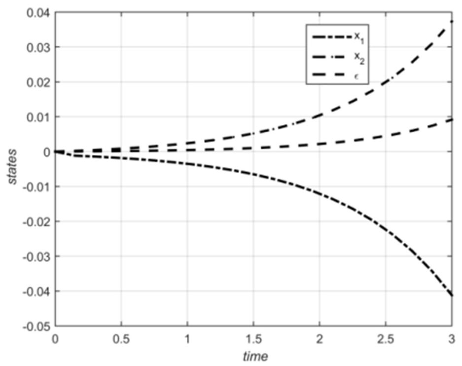
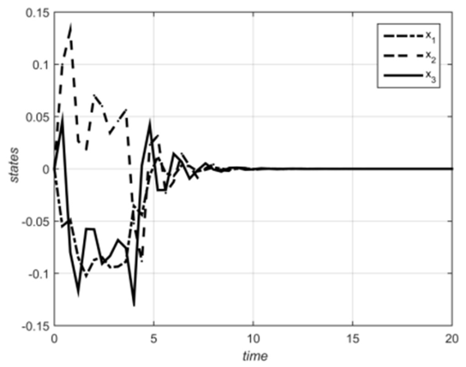
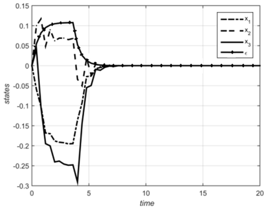
5. Numerical Examples

The applicability of the finite time reduced order H∞ controller design approach proposed in this paper is shown in this section by three numerical examples.
Example 1. 
In this example, the magnetic-tape-drive servo system in the paper [44] is used to verify the proposed approach. Let the sampling rate T s = 0.05 , and with the assumption that the disturbance is constant during each sampling period, we have the discretized system (1) with the following matrices:
A = 0.9599           0.0401     0.4861 0.0139 0.0401           0.9599       0.0139 0.4861 0.1566   0.1566             0.9321 0.0679 0.1566 0.1566 0.0679               0.9321 ,   B = D x = 0.1049             0.0017 0.0017               0.1049 0.4148   0.0118 0.0118             0.4148
Applying the stability results presented in the proposed approach and [44], the corresponding state-feedback gains are obtained. In this paper, we found that the controller gain is
K u = 0.0561 0.0724 0.0724 0.0561
while its value in the paper [42] is
K = 0.2717 0.2810 0.2810 0.2717
Then, it is clear that the control law gain obtained in this paper is less than that obtained in [42]. Consequently, the approach proposed in this paper is less conservative in stabilizing the closed-loop system compared to [44].
Finally, it is illustrated how, by using the proposed approach, a control law can be obtained which is simple to implement in a control system using state variables x k , which provides stability in many cases, with good transient responses and feasible control signals.
Example 2. 
Let us consider now the following matrices:
A = 1.5 0.2 0 1.2 ,     B = 0.25 0 , C y = 1 1 ,     C z = 1 1 ,   D x = 0.001 3 2 ,     D y = 0.01 ,     D z = 0.01
Then, the application of the proposed algorithm allows us to have:
R = 1 0 0 1 ,     c 2 = 1.18 ,     γ = 0.99 ,   d = 1 ,     N = 3 ,     α = 1.45
Using the LMI tools of MATLAB, applying the conditions obtained in this article, and solving the matrices (12) and (13), we obtain:
X = 1.0016 0.3121 0.3121 0.3051 , Y = 4.2175 0.1236
where w k = 0.1 ,   k 1 , N , and so we obtain:
K u = 5.9961 5.7296
On the other hand, we have:
P = 17.0503 17.4008 17.4008 46.3613 ,   Q = 46.9138 , Y = 55.8461 113.8726 156.2189
Thus, the gain matrix Z ¯ = Q 1 Y is applied where
Z ¯ = 1.1904 2.4273 3.3299
In the end, the values of A f , K , G , and L f are given by:
A f = 1.233 ,     K = 5.9082 , G = 0.0220 , L f = 0.0235
Then, the H∞ performance is verified where
k = 0 N z T k z k = 1.6574 × 10 5 γ 2 k = 0 N w T k w k = 0.1960
Finally, the trajectories evolution of the states’ variables are given in Figure 1. Thus, the system is not asymptotically stable, simply because it has been represented for a prescribed time interval and then the studied system can be said to be stable for a limited time using the H∞ reduced order controller parameters of the proposed approach.
Then, it can be seen from Figure 1 that the state responses of the considered system converge to the equilibrium point as it reaches the desired tracking performance. Then, it is confirmed that the equilibrium point of this system is stable over a finite time interval. Therefore, this figure proves that the FTB-H∞ of the closed-loop system is guaranteed, and the effectiveness of our results is verified. Consequently, the simulation results show the accuracy and the effectiveness of the proposed approach for which the closed-loop system is asymptotically stable.
Example 3. 
The matrices considered in this example are given by:
A = 0.1032 0.1096 0.9374 0.8785 0.6190 0.6571 0.8668 0.4123 0.8172 ,   B = 1 0 1 T
D x = 0 1 1 T ,   D y = 1 ,     D z = 0 0 1 T ,     C y = 0 1 1 ,     C z = I
Then, let R = I ,   d = 1 ,   N = 20 ,   α = 1.001 , and c 2 = 1.18 .
Applying the adopted algorithm, we obtain the following filter-based controller matrices:
A f = 0.4889 ,     K = 0.5943 ,   G = 0.4854 ,     L f = 0.3115
In order to study the convergence performance of the proposed approach, some simulation results are presented in Figure 2 where
w k = 0.1           i f             k 4 0                   i f             k > 4  
Also, the H∞ performance is verified in this case with
k = 0 N z T k z k = 0.6095 γ 2 k = 0 N w T k w k = 0.8100
It is then observed that these trajectories rapidly converge towards the operating point and that the disturbances are correctly decoupled. Thus, the simulation results demonstrate the efficiency of the proposed controller, for which the control loop system is asymptotically stable despite significant disturbances; therefore, the desired responses are obtained.
In order to compare the performance of the proposed approach with that reported in the literature, the simulation results of [40] are given in Figure 3 where γ = 0.286 .
From these figures, we can clearly see that our methodology provides better performance with shorter convergence time and rejects the disturbances faster compared to [15]. Using our new approach, the best controller parameters are obtained compared to the reference [15] which guarantees the FTB-H∞ and the robust stability of the closed-loop system despite the significant disturbances. In general, the results are significantly improved in this paper, and therefore they are better compared to those obtained in the paper [15].
Finally, we can say that the developed results show a high agreement with theoretical predictions to attain the specified performance and a big improvement over previous efforts within the literature.
Remark 10. 
Despite the presence of external disturbances during the interval 0 , N , efficient conditions are provided to achieve the desired performance, where the studied closed-loop system is stabilized by an H∞ reduced order controller in finite time. It follows that the sum of errors from 0 to N is the same as from 0 to (i.e, i = 0 N e T i e i = i = 0 e T i e i ).
Remark 11. 
Based on what has been mentioned (Remark 8, Example 1, Example 2, Example 3, …), we can say that our results, although endowed with FTS, are less restrictive than those with finite time and infinite time stability presented in the literature.On the other hand, the obtained results do not make us lose sight of other issues and challenges that need to be taken into account, among them delays and saturated inputs.

6. Conclusions

In this paper, a new approach to designing a reduced-order H∞ controller is given for discrete-time systems. The aim is to guarantee the FTS despite external disturbances. The resulting conditions, which are given in the form of LMIs, depend on the results of parametrization of the algebraic constraints easily obtained from the conditions of unbiased estimation error. Similarities and differences between this paper and those given in the literature, as well as illustrative examples, were given to best understand the approach. The obtained results show a high agreement with the theoretical expectations, thus reaching the required performances and obtaining significant improvement compared to previous efforts mentioned in the literature. In fact, very good transient responses were obtained. On the other hand, the proposed methodology opens up new topics for research: the future lines of research are to extend the adopted approach to other systems closely related to what we are studying, such as nonlinear, data samples, etc. Additionally, the approach has significant results for future research and we can now solve practical control problems. Moreover, the description and modeling of the process is more realistic because it presents a more interesting control problem and can then provide insight for future research on the same topic. This is an important step to frame this type of problem in a more formal, yet realistic context, enabling it to address important service directives.

Author Contributions

Conceptualization, M.T.; methodology, M.T. and N.E.F.; software, N.E.A.; validation, M.T. and A.B.; formal analysis, M.T. and N.E.F.; investigation, M.T.; resources, M.T.; data curation, M.T.; writing—original draft preparation, M.T.; writing—review and editing, A.B., R.F. and M.A.-A.; visualization, E.H.T.; supervision, E.H.T., N.E.F., A.B. and M.A.-A.; project administration, M.T.; funding acquisition, M.A.-A. All authors have read and agreed to the published version of the manuscript.

Funding

This research received no external funding.

Institutional Review Board Statement

Not applicable.

Informed Consent Statement

Not applicable.

Data Availability Statement

Not applicable.

Conflicts of Interest

The authors declare no conflict of interest.

References

  1. Baleanu, D.; Sajjadi, S.S.; Jajarmi, A.; Defterli, Ö. On a nonlinear dynamical system with both chaotic and nonchaotic behaviors: A new fractional analysis and control. Adv. Differ. Equ. 2021, 34, 1–17. [Google Scholar] [CrossRef]
  2. Baleanu, D.; Sajjadi, S.S.; Asad, J.H.; Jajarmi, A.; Estiri, E. Hyperchaotic behaviors, optimal control, and synchronization of a nonautonomous cardiac conduction system. Adv. Differ. Equ. 2021, 157, 1–24. [Google Scholar] [CrossRef]
  3. Baleanu, D.; Zibaei, S.; Namjoo, M.; Jajarmi, A. A nonstandard finite difference scheme for the modeling and nonidentical synchronization of a novel fractional chaotic system. Adv. Differ. Equ. 2021, 308, 1–19. [Google Scholar] [CrossRef]
  4. Jajarmi, A.; Baleanu, D.; Vahid, K.Z.; Mobayen, S. A general fractional formulation and tracking control for immunogenic tumor dynamics. Math. Methods Appl. Sci. 2022, 45, 667–680. [Google Scholar] [CrossRef]
  5. Jajarmi, A.; Pariz, N.; Effati, S.; Kamyad, A.V. Infinite horizon optimal control for nonlinear interconnected large-scale dynamical systems with an application to optimal attitude control. Asian J. Control 2012, 14, 1239–1250. [Google Scholar] [CrossRef]
  6. El Fezazi, N.; El Fakir, Y.; Bender, F.A.; Idrissi, S. AQM congestion controller for TCP/IP networks: Multiclass traffic. J. Control Autom. Electr. Syst. 2020, 31, 948–958. [Google Scholar] [CrossRef]
  7. El Fezazi, N.; Frih, A.; Lamrabet, O. New H∞ dynamic observer design for time-delay systems subject to disturbances. Int. J. Syst. Sci. 2020, 51, 2610–2624. [Google Scholar]
  8. El Fezazi, N.; Tissir, E.H.; El Haoussi, F.; Bender, F.A.; Husain, A.R. Controllersynthesisforsteer-by-wiresystemperformanceinvehicle. Iran. J. Sci. Technol. Trans. Electr. Eng. 2019, 43, 813–825. [Google Scholar] [CrossRef]
  9. Lamrabet, O.; El Fezazi, N.; El Haoussi, F.; Tissir, E.H.; Alvarez, T. Congestion control in TCP/IP routers based on sampled-data systems theory. J. Control Autom. Electr. Syst. 2020, 31, 588–596. [Google Scholar] [CrossRef]
  10. Yi, X.; Guo, R.; Qi, Y. Stabilization of chaotic systems with both uncertainty and disturbance by the UDE-based control method. IEEE Access 2020, 8, 62471–62477. [Google Scholar] [CrossRef]
  11. Gao, N.; Darouach, M.; Alma, M. Dynamic observer design for a class of nonlinear systems. In Proceedings of the 3rd Advanced Information Technology, Electronic and Automation Control Conference, Chongqing, China, 12–14 October 2018; pp. 373–376. [Google Scholar]
  12. Xiong, X.; Pal, A.K.; Liu, Z.; Kamal, S.; Huang, R.; Lou, Y. Discrete-timeadaptivesuper-twistingobserverwithpredefinedarbitraryconvergencetime. IEEE Trans. Circuits Syst. II Express Briefs 2020, 68, 2057–2061. [Google Scholar]
  13. Zang, J.; Chen, X.; Hao, F. Observer-based event-triggered bipartite consensus of linear multi-agent systems. Int. J. Control Autom. Syst. 2021, 19, 1291–1301. [Google Scholar] [CrossRef]
  14. Zare, K.; Shasadeghi, M.; Izadian, A.; Niknam, T.; Asemani, M.H. Switching TS fuzzy model-based dynamic sliding mode observer design for non-differentiable nonlinear systems. Eng. Appl. Artif. Intell. 2020, 96, 103990. [Google Scholar] [CrossRef]
  15. Kalman, R.E. A new approach to linear filtering and prediction problems. J. Basic Eng. 1960, 82, 35–45. [Google Scholar] [CrossRef] [Green Version]
  16. Luenberger, D. An introduction to observers. IEEE Trans. Autom. Control 1971, 16, 596–602. [Google Scholar] [CrossRef]
  17. Li, H.; Wu, C.; Yin, S.; Lam, H.K. Observer-based fuzzy control for nonlinear networked systems under unmeasurable premise variables. IEEE Trans. Fuzzy Syst. 2016, 24, 1233–1245. [Google Scholar] [CrossRef] [Green Version]
  18. Qiu, J.; Sun, K.; Wang, T.; Gao, H. Observer-based fuzzy adaptive event-triggered control for pure-feedback nonlinear systems with prescribed performance. IEEE Trans. Fuzzy Syst. 2019, 27, 2152–2162. [Google Scholar] [CrossRef]
  19. Venkatesh, M.; Patra, S.; Ray, G. Observer-based controller design for linear time-varying delay systems using a new Lyapunov-Krasovskii functional. Int. J. Autom. Control 2021, 15, 99–123. [Google Scholar] [CrossRef]
  20. Wang, X.; Yu, H.; Hao, F. Observer-based disturbance rejection for linear systems by aperiodical sampling control. IET Control Theory Appl. 2017, 11, 1561–1570. [Google Scholar] [CrossRef]
  21. Boutat-Baddas, L.; Osorio-Gordillo, G.L.; Darouach, M. H∞ dynamic observers for a class of nonlinear systems with unknown inputs. Int. J. Control 2021, 94, 558–569. [Google Scholar] [CrossRef]
  22. Gao, N.; Darouach, M.; Voos, H.; Alma, M. New unified H∞ dynamic observer design for linear systems with unknown inputs. Automatica 2016, 65, 43–52. [Google Scholar] [CrossRef]
  23. Wang, L.; Wang, H.; Liu, P.X.; Ling, S.; Liu, S. Fuzzy finite-time command filtering output feedback control of nonlinear systems. IEEE Trans. Fuzzy Syst. 2020, 30, 97–107. [Google Scholar] [CrossRef]
  24. Darouach, M.; Zasadzinski, M. Optimal unbiased reduced order filtering for discrete-time descriptor systems via LMI. Syst. Control Lett. 2009, 58, 436–444. [Google Scholar] [CrossRef] [Green Version]
  25. Kim, K.S.; Rew, K.H. Reduced order disturbance observer for discrete-time linear systems. Automatica 2013, 49, 968–975. [Google Scholar] [CrossRef]
  26. Vaidyanathan, S.; Madhavan, K. Reduced order linear functional observers for large scale linear discrete-time control systems. In Proceedings of the 4th International Conference on Computing, Communications and Networking Technologies, Tiruchengode, India, 4–6 July 2013; pp. 1–7. [Google Scholar]
  27. Wang, Y.; Sun, M.; Wang, Z.; Liu, Z.; Chen, Z. A novel disturbance-observer based friction compensation scheme for ball and plate system. ISA Trans. 2014, 53, 671–678. [Google Scholar] [CrossRef]
  28. Chen, L.; Wang, Q. Finite-time adaptive fuzzy command filtered control for nonlinear systems with indifferentiable non-affine functions. Nonlinear Dyn. 2020, 100, 493–507. [Google Scholar] [CrossRef]
  29. Fu, C.; Wang, Q.G.; Yu, J.; Lin, C. Neural network-based finite-time command filtering control for switched nonlinear systems with backlash-like hysteresis. IEEE Trans. Neural Netw. Learn. Syst. 2020, 32, 3268–3273. [Google Scholar] [CrossRef]
  30. Zhang, Y.; Shi, P.; Nguang, S.K. Observer-based finite-time H∞ control for discrete singular stochastic systems. Appl. Math. Lett. 2014, 38, 115–121. [Google Scholar] [CrossRef]
  31. Zhang, Y.; Shi, P.; Nguang, S.K.; Karimi, H.R. Observer-based finite-time control for discrete fuzzy jump nonlinear systems with time delays. In Proceedings of the American Control Conference, Washington, DC, USA, 17–19 June 2013; pp. 6394–6399. [Google Scholar]
  32. Bhiri, B.; Delattre, C.; Zasadzinski, M.; Abderrahim, K. A descriptor system approach for finite-time control via dynamic output feedback of linear continuous systems. IFAC-Pap. 2017, 50, 15494–15499. [Google Scholar] [CrossRef]
  33. Bhiri, B.; Delattre, C.; Zasadzinski, M.; Abderrahim, K. Results on finite-time boundedness and finite-time control of non-linear quadratic systems subject to norm-bounded disturbances. IET Control Theory Appl. 2017, 11, 1648–1657. [Google Scholar] [CrossRef]
  34. Bhiri, B.; Delattre, C.; Zasadzinski, M.; Souley-Ali, H.; Zemouche, A.; Abderrahim, K. Finite time H∞ controller design based on finite time H∞ functional filter for linear continuous systems. In Proceedings of the 4th International Conference on Systems and Control, Sousse, Tunisia, 28–30 April 2015; pp. 460–465. [Google Scholar]
  35. Delattre, C.; Bhiri, B.; Zemouche, A.; Souley-Ali, H.; Zasadzinski, M.; Abderrahim, K. Finite-time H∞ functional filter design for a class of descriptor linear systems. In Proceedings of the 22nd Mediterranean Conference on Control and Automation, Palermo, Italy, 16–19 June 2014; pp. 1572–1577. [Google Scholar]
  36. Amato, F.; Carbone, M.; Ariola, M.; Cosentino, C. Finite-time stability of discrete-time systems. In Proceedings of the 2004 American Control Conference, Boston, MA, USA, 30 June–2 July 2004; Volume 2, pp. 1440–1444. [Google Scholar]
  37. Amato, F.; Ariola, M. Finite-time control of discrete-time linear systems. IEEE Trans. Autom. Control 2005, 50, 724–729. [Google Scholar] [CrossRef]
  38. Cheng, J.; Zhu, H.; Zhong, S.; Zhang, Y. Finite-time boundness of H∞ filtering for switching discrete-time systems. Int. J. Control. Autom. Syst. 2012, 10, 1129–1135. [Google Scholar] [CrossRef]
  39. Darouach, M. H∞ Unbiased Filtering for Linear Descriptor Systems via LMI. IEEE Trans. Autom. Control 2009, 54, 1966–1972. [Google Scholar] [CrossRef] [Green Version]
  40. Du, X.; Yang, G. Improved LMI conditions for H∞ output feedback stabilization of linear discrete-time systems. Int. J. Control Autom. Syst. 2010, 10, 163–168. [Google Scholar] [CrossRef]
  41. Lee, Y.S.; Han, S.H.; Kwon, W.H. H2/H∞FIR Filters for Discrete-time State Space Models. Int. J. Control Autom. Syst. 2006, 4, 645–652. [Google Scholar]
  42. O’Brien, R.T., Jr.; Kiriakidis, K. Reduced-order H∞ filtering for discrete-time, linear, time-varying systems. In Proceedings of the American Control Conference, Boston, MA, USA, 30 June–2 July 2004; pp. 4120–4125. [Google Scholar]
  43. Xu, D.; Wu, D.; Hu, A.; Wu, S. Robust Unbiased Filtering for System with Unknown System Noise Input. J. Comput. Inf. Syst. 2012, 8, 3867–3877. [Google Scholar]
  44. Zhang, J.; Shi, P.; Xia, Y.; Yang, H. Discrete-time sliding mode control with disturbance rejection. IEEE Trans. Ind. Electron. 2018, 66, 7967–7975. [Google Scholar] [CrossRef]
Figure 1. Trajectories of the closed-loop system states.
Mathematics 11 00031 g001
Figure 2. Trajectories of the states (the proposed approach).
Mathematics 11 00031 g002
Figure 3. Trajectories of the states.
Mathematics 11 00031 g003
Disclaimer/Publisher’s Note: The statements, opinions and data contained in all publications are solely those of the individual author(s) and contributor(s) and not of MDPI and/or the editor(s). MDPI and/or the editor(s) disclaim responsibility for any injury to people or property resulting from any ideas, methods, instructions or products referred to in the content.

