Robust Stability Analysis of Filtered PI and PID Controllers for IPDT Processes

Abstract

The paper discusses the stability and robustness of the proportional-integral (PI), proportional-integral-derivative (PID), and proportional-integral-derivative-accelerative (PIDA) controller for the integral-plus-dead-time (IPDT) plants. To enable the implementation and measurement of noise attenuation, binomial low-pass filters are added to the traditional design of controllers with ideal transfer functions, and the impact of the low-pass filters on the robust stability of the circuit is studied in detail. The proposed controller tuning, which integrates the suboptimal controller and filter design, is based on explicit tuning formulas derived by using the multiple real dominant pole (MRDP) method. It is shown that by combining derivative actions with possibly higher-order low-pass filters, it is possible to either accelerate the transients or increase the closed loop robustness and that the problem of defining the robust stability area should be addressed at the stage of determining the process model. In addition, if wishing to maintain the closed loop robustness of unfiltered PI control, while increasing the degree of the derivative components, one needs to increase the filtering properties of the low-pass filter used accordingly. Simple analytical relations for setting filtered PI, PID, and PIDA controllers with equivalent robustness are derived.

1. Introduction

PID controllers remain the most widely used technology for industrial process control. However, some aspects of controller design deserve even more attention. For example, the design of derivative filters, which are required to implement proportional-integral-derivative (PID) control in practice, can prove to be found a troublesome problem, leading to a trivial solution of eliminating derivative action and using only the simplest PI control. Since the design of a filtered controller requires much more effort than the design of an ideal controller without a filter, textbooks are flooded with sentences such as that the derivative part is the most difficult to tune [1], or that the derivative action is not appropriate for noisy and time-delayed processes [2]. On the other hand, signal filtering becomes very important not only for controllers with derivative action [3,4,5,6,7,8,9]. Indeed, the measurement noise also has significant effects on the control accuracy, energy consumption, heat dissipation, actuator wear, unwanted vibration, acoustic noise, etc.

Through simulation and experiments on real processes, it was possible to show that the design of filters can be included in the task of optimal tuning of controllers using the method of multiple real poles [10,11]. From the point of view of damping the noise, optimal results were given by filters with a higher order than the order of the used derivative term. However, with respect to filtering, some authors object that using higher-order filters is not practical from a discrete-time perspective, and similar results can be obtained by using a first-order low-pass filter and ensuring that a good sensor is used for control. Despite technological advances, until today, low-pass filters only attenuate noise, they cannot remove noise, even though higher-orders are used. As a counter-argument, it can be argued that the higher speed of microprocessors and A/D converters is narrowing the gap between analog and digital implementations. Moreover, digital controllers are still not the only possible approach and in addition to traditional analog controllers (especially for fast processes), newer approaches, such as Field Programmable Analog Arrays (FPAA) [12,13,14] show promising results for analog implementations. By considering higher-order filters, we open the space for the use of controllers with higher-order derivative components [15,16]. When proposing to use sensors with the lowest possible measurement noise, it should be noted that such a solution is either costly or increases the sensor time constant. Control solutions should be provided for the existing non-ideal measurement devices.

As indicated by quotations of older references from one of the first textbooks of automatic control [17], the multiple real dominant pole (MRDP) method belongs to the oldest methods of optimal adjustment of controllers for time-delayed systems [18,19,20,21,22]. Although even with the help of a simple performance portrait method [23,24,25] it is possible to show that from the point of view of the resulting dynamics of the circuit, slightly better results can be achieved based on complex conjugate poles. More rigorously, similar problems have also been treated by the latest research in the field of the maximum decay rate of the closed-loop response for linear time-invariant time-delay systems [26,27], also giving a more detailed review of the latest research from this area. However, the ease of use of the MRDP method is a great advantage, especially in the case of the analytical design of controllers with higher order derivatives [15], which can further be modified for constrained control design based on the series PID controllers [28], including an explicit observer of input disturbances [29,30,31]. Recently, it was shown that a new integrated filter and controller tuning allows one to deal with filters of an arbitrarily chosen order n, which gives much better results than the traditional derivative filter design. It allowed tuning of filtered PI and PID controllers [19]; the less common PIDD${}^2$ (PIDA) or PIDD${}^2$D${}^3$ controllers with higher order derivative actions, up to the general-order controller using the simple notation of PID${}_n^m$ control. By applying the derivative actions up to a degree $m;m=0,1,2,\cdots ;m\le n$ the excessive control effort is simultaneously reduced and the transient speed increased while the control signals remain sufficiently smooth [15,32,33]. By consistently using integer, possibly higher-order derivatives and filters, the presented design differs from fractional-order PIDs [34]. With them, it is possible to use non-integer operators of derivation and integration, and the designed controllers are finally approximated by filters of higher orders.

In this paper, we extend the design of filtered PI, PID, and PIDA controllers for the integral plus time delay (IPDT) plant from [15,35] with robust stability evaluation considering $m=0,1,2$. In evaluating robustness, while taking into account the arguments given in [36,37,38], the article avoids the calculations based on peak sensitivity functions typically used in PID control or other advanced studies (such as treated in [39]), and focuses instead on robust stability, which is explained, for example, in [40].

In this context, the paper is organized as follows. Section 2 summarizes the main results of the ideal PID${}^m$ controller design for the IPDT plant for $m=0,1$ and 2 from [15]. The controller extension by binomial filters of the order $n\ge m$ is also described to obtain fully implementable, proper, or strictly proper controllers. Section 3 presents the robust stability problem, which is solved in Section 4 for unfiltered and filtered PI control. The robust stability analysis of the filtered PID and PIDA controllers is then addressed in Section 5 and Section 6. The main results of the work and future developments are summarized in the conclusions.

2. PI, PID, and PIDA Controller for the IPDT Plant Tuned with the MRDP Method

In this paper, the velocity of the transients is evaluated using the absolute integral error

$$IAE={\int }_0^{\infty }\left|e\left(t\right)\right|dt;e=w-y$$

(1)

To keep the paper short, the evaluation deals only with the step responses of the input disturbance, with all corresponding performance values denoted by the subscript “d”.

For the process output $y\left(t\right)$ and the controller output $u\left(t\right)$, the robustness analysis will focus on an IPDT process model described by the transfer function

$$S\left(s\right)=\frac{Y\left(s\right)}{U\left(s\right)}=S_0\left(s\right)e^{-T_{dp}s};S_0\left(s\right)=\frac{K_{sp}}{s};K_{sp}\ne 0;T_{dp}\ge 0$$

(2)

with a gain $K_{sp}$ and a dead time $T_{dp}$. In the “optimal” controller tuning, the omitted plant model index “p” corresponds to the “nominal” model parameters $K_s$ and $T_d$.

2.1. Optimal “Ideal” Controller Design

To illustrate problems of the process modeling mentioned (without some deeper analysis) already in [28], in the following, we start with summarizing the main results of deriving the optimal parameters of PI, PID, and PIDA controllers from [15], which will later be used to evaluate the robustness of the filtered PI, PID and PIDA controllers tuned by the MRDP method. Where appropriate, we will refer to these controllers simply as PI, PID, and PIDA, but in the case of efficiency (mainly in the treatment of filtered control), we will also use the more detailed generalized designation of these controllers from the article [15] in the form of $PI{D}_n^m$. Controllers with higher derivatives $m>2$ will be treated in a special article.

Parallel PI, PID, and PIDA control can be specified by a transfer function

$$\begin{array}{c}PI{D}^m\left(s\right)=K_c\left[{\displaystyle \frac{1+T_{im}s}{T_{im}s}}+T_{D1}s+T_{D2}^2{s}^2\right]=K_{cm}+{\displaystyle \frac{K_{im}}{s}}+K_{D1m}s+K_{D2m}{s}^2;\hfill \\ m=0,1,2\hfill \end{array}$$

(3)

For $m\ge 1$ such a controller needs a filter, which will be treated later. For the nominal plant parameters and the most complex controller $PI{D}^2\left(s\right)=C\left(s\right)$ corresponding to $m=2$ (for the sake of simplicity, the index m has been omitted), the disturbance-to-output transfer function is

$$\begin{array}{c}{F}_{dy}\left(s\right)=Y\left(s\right)/D_i\left(s\right)={\displaystyle \frac{S\left(s\right)}{1+C\left(s\right)S\left(s\right)]}}=\hfill \\ ={\displaystyle \frac{K_s{T}_{i}s}{T_i{s}^2{e}^{T_{d}s}+K_c{K}_s[1+s{T}_i(1+T_{D1}s+T_{D2}^2{s}^2)]}}\hfill \end{array}$$

(4)

Similarly, for example in [41], a simplified system expression can be based on dimensionless parameters

$$\begin{array}{c}p=s{T}_d;K=K_c{K}_s{T}_d;{\tau }_i={\displaystyle \frac{T_i}{T_d}};{\tau }_1={\displaystyle \frac{T_{D1}}{T_d}};{\tau }_2={\left({\displaystyle \frac{T_{D2}}{T_d}}\right)}^2\hfill \end{array}$$

(5)

For (4) it yields

$$\begin{array}{c}{F}_{dy}\left(p\right)={\displaystyle \frac{1}{K_c}}{\displaystyle \frac{K{\tau }_{i}p}{{\tau }_i{p}^2{e}^p+K[1+s{\tau }_i(1+{\tau }_{1}p+{\tau }_2^2{p}^2)]}}\hfill \end{array}$$

(6)

This means that, in addition to dimensionless parameters (5), the standardized disturbance response also depends on the current value of $K_s$ or $K_c=K/\left(K_s{T}_d\right)$. For PID control ${\tau }_2=0$ and for PI ${\tau }_1={\tau }_2=0$.

Optimal controller parameters determined by the MRDP method guarantee the $(m+2)$-tuple real dominant pole $p_o$

$$\begin{array}{c}{p}_o=s_o{T}_d=\sqrt{m+2}-(m+2)\hfill \end{array}$$

(7)

Thereby, the $(m+2)$ controller parameters of the normed quasi-polynomial

$$P\left(p\right)={\tau }_i{p}^2{e}^p+K_o[1+p{\tau }_i(1+{\tau }_{1}p+{\tau }_2{p}^2)]$$

(8)

are determined to get an $(m+2)$-tuple real dominant pole $p_o$ fulfilling equations

$$\begin{array}{c}{\left[P\left(p\right)=0;{\displaystyle \frac{dP\left(p\right)}{dp}}=0;\cdots ;{\displaystyle \frac{d^{m+2}P\left(p\right)}{d{p}^{m+2}}}=0\right]}_{p=p_o}\hfill \end{array}$$

(9)

From ${\displaystyle \frac{d^{m+2}P\left(p\right)}{d{p}^{m+2}}}=\left(p^2+2(m+2)p+(m+2)(m+1)\right)$ the dominant pole is chosen as the solution of $d^{m+2}P\left(p\right)/d{p}^{m+2}=0$ which is the closest to the origin.

The use of the dimensionless parameters (5) simplifies the optimal controller calculation, especially the differentiation of $P\left(p\right)$. For $m\in [0,2]$ the corresponding values $K,{\tau }_i,{\tau }_1,{\tau }_2$ are summarized in

Table 1. Optimal PID${}^m$ parameters corresponding to (5) and (7), $m\in [0,2]$.

	$\mathit{m}=0$	$\mathit{m}=1$	$\mathit{m}=2$
K	0.4612	0.78361	1.08268
${\tau }_i$	5.8284	3.73205	3.00000
${\tau }_1$	0	0.26289	0.37500
${\tau }_2$	0	0	0.04167

. For a more detailed derivation see [15] (or also [42]).

Reasons for using the derivative action may be demonstrated by the optimal integral of error ($IE$) values equal for the considered case to the integral of absolute error ($IAE$)

$$IA{E}_d=T_i/K_c=K_s{T}_d^2{\overline{IAE}}_d$$

(10)

As expressed by the index “d”, they are corresponding to unit input disturbance step responses. Under the assumption of a not changing sign of the control error, they may be derived as $IAE=IE$.

Obviously, with increasing parameter m the $IA{E}_d$ values decrease.

By increasing m from 0 to 1, the dimensionless value ${\overline{IAE}}_d$ (see

Table 2. Optimal normed ${\overline{IAE}}_d=IA{E}_d/\left(K_s{T}_d^2\right)$ values corresponding to unit input disturbance step responses for PID${}^m$ from Table 1.

-	$\mathit{m}=0$	$\mathit{m}=1$	$\mathit{m}=2$
${\overline{IAE}}_d$	12.639	4.763	2.771

) decreases more than 2 times and from 0 to 2 more than $4.5$ times.

When wishing to examine the most important question, how far such improvements can be achieved in real situations, we have to replace ideal PID${}^m$ controllers with a filtered PID${}_n^m$ control. The total loop delay, including filtration, will be expressed in terms of the plant dead time $T_{dp}$ increased by the equivalent amount $T_e$ spent on filtration.

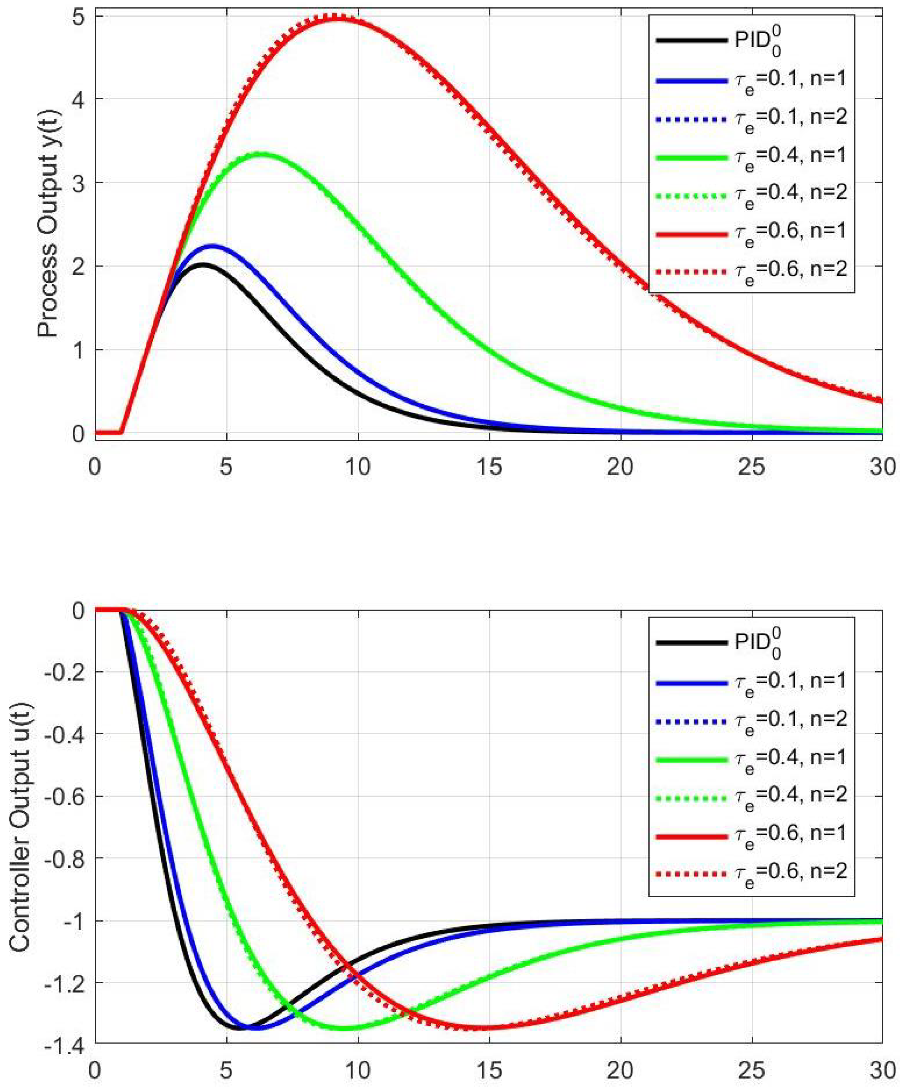
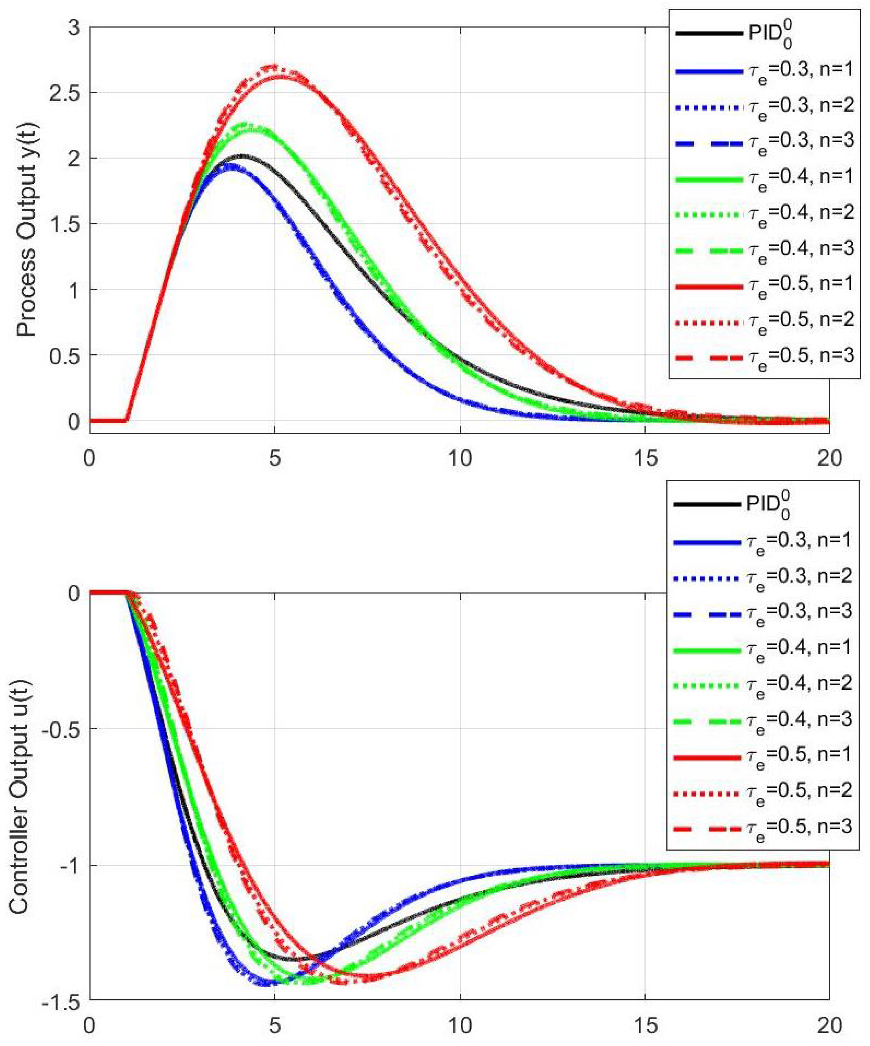
2.2. PID Controllers with Proper Transfer Functions and the Delay Equivalence

To get implementable solutions, the above derived “ideal” controllers can be simply augmented by an nth order binomial filter

$$Q_n\left(s\right)=1/{\left(T_{f}s+1\right)}^n;n=1,2,\cdots ;n\ge m$$

(11)

The resulting transfer function $PI{D}_n^m\left(s\right)=PI{D}^m\left(s\right)Q_n\left(s\right)$ becomes proper for $n=m$. However, the measurement noise is significantly more attenuated for $n>m$. Of course, we will pay for a better smoothing of the noise by slowing down the transient responses. However, an important question will be how the selection of different filters in combination with the derivative action will affect the robustness of the circuit.

For a long time, one of the most important reasons leading to the already mentioned textbook comments [1,2] on the PID derivative action was given by the absence of simple and reliable methods for its filter tuning. Even the newest works in this area consider different filters for different components of the control signal, which further complicates their optimal setting [9,43,44].

One possible solution to include the filter design in the optimal controller tuning is based on the equivalence of n time constants $T_f$ of $Q_n\left(s\right)$ with an equivalent dead time $T_e$, which can then be added to the process dead-time $T_{dp}$, i.e., when the considered dead-time $T_d$ consists of an estimate of the loop delay $T_{dp}$ (representing the sum of the process, actuator, and measurement sensor delays with a communication and computation delay) and an intentionally introduced equivalent filter delay estimate $T_e$

$$T_d=T_{dp}+T_e$$

(12)

$T_e$ can be approximated as (see e.g., [45])

$$T_e=nN{T}_f$$

(13)

The coefficient N can be specified by values ranging from $N=0.5$ (equivalence based on “half rule”) to $N=1$ (equivalence based on “average residence time”).

3. Robustness Issues

As documented by numerous approaches, the integral models represent more general and cruder linear approximations allowing simple robust control design of a broad class of non-linear, time-varying, and uncertain systems (see e.g., the controller tuning by Ziegler and Nichols [46], the “model-free control” by Fliess and coworkers [47], the “active-disturbance-rejection-control” developed by Han and Gao [48], the robust control proposed by Mercader and coworkers [49], or the design in [50] to mention just a few of them). Regardless of whether known or not, the system’s internal feedback gets here into the role of an uncertainty compensated together with external input disturbances, which significantly simplifies the controller design. Next, we will analyze, how a possible mismatch of the plant and model parameters influences the closed-loop stability.

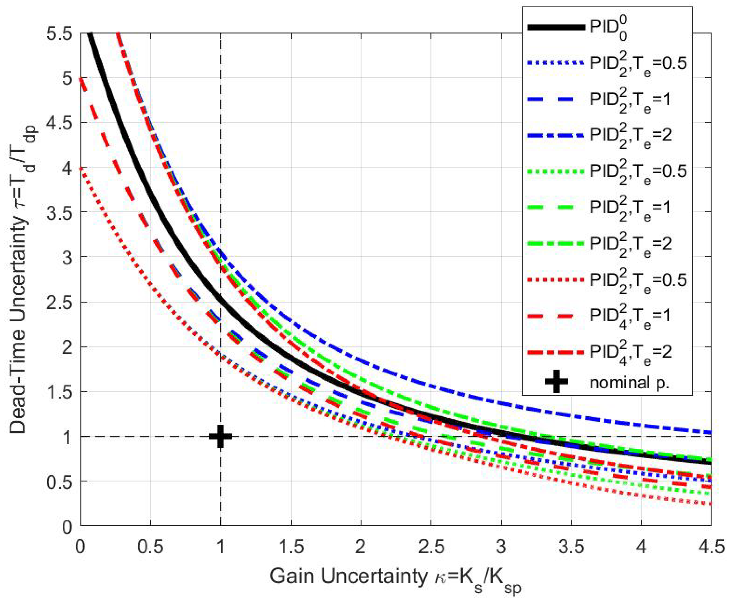
Robust Stability Analysis

The stability analysis will be based on the characteristic quasi-polynomial of the loop, and a modification of the D-decomposition [51], or the parameter space method [40]. It is looking for critical controller parameters corresponding to a pole $p=j\Omega ,\Omega \in [0,\infty )$ at the imaginary axis

$$P(j\Omega )=-T_i{\Omega }^2{(1+j\Omega T_f)}^n{e}^{j\Omega T_d}+K_c{K}_s[1+j\Omega T_i(1+j\Omega T_{D1}-{\Omega }^2{T}_{D2}^2)]$$

(14)

it allows one to split a complex characteristic equation into two simpler real equations.

For the controller tuning

$$\begin{array}{c}{T}_d=T_{dp}+T_e;K_c=\frac{K}{K_{sp}(T_{dp}+T_e)};\hfill \\ T_i={\tau }_i(T_{dp}+T_e);T_{D1}={\tau }_1(T_{dp}+T_e);T_{D2}={\tau }_2{(T_{dp}+T_e)}^2\hfill \end{array}$$

(15)

and the positive dimensionless variables

$$\begin{array}{c}\omega =\Omega (T_{dp}+T_e);{\tau }_e={\displaystyle \frac{T_e}{T_{dp}+T_e}};{\tau }_f={\displaystyle \frac{T_f}{T_{dp}+T_e}}\hfill \\ \tau ={\displaystyle \frac{T_d}{T_{dp}}};\overline{\tau }={\displaystyle \frac{T_d}{T_{dp}+T_e}}={\displaystyle \frac{\tau T_{dp}}{T_{dp}+T_e}};\hfill \\ \kappa ={\displaystyle \frac{K_s}{K_{sp}}};{\tau }_1={\displaystyle \frac{T_{D1}}{T_{dp}+T_e}};{\tau }_2={\left({\displaystyle \frac{T_{D2}}{T_{dp}+T_e}}\right)}^2\hfill \end{array}$$

(16)

the quasi-polynomial (14) can be expressed as

$$\begin{array}{c}P\left(j\omega \right)=-{\tau }_i{\omega }^2{(1+j\omega {\tau }_f)}^n{e}^{j\omega \overline{\tau }}+\kappa [1+j\omega {\tau }_i(1+j\omega {\tau }_1-{\omega }^2{\tau }_2)]\hfill \end{array}$$

(17)

4. Robust Stability of PI Controllers

4.1. Unfiltered PI Controllers

In the simplest case of an unfiltered PI controller with $m=n=0$, ${\tau }_e=0$ and $\overline{\tau }=\tau$ it will be

$$P\left(j\omega \right)=-{\tau }_i{\omega }^2{e}^{j\omega \tau }+\kappa K(1+j\omega {\tau }_i)$$

(18)

This complex quasi-polynomial can be used to formulate two real equations corresponding to the stability border

$$\begin{array}{c}-{\tau }_i{\omega }^{2}cos\left(\omega \tau \right)+\kappa K=0\hfill \\ -{\tau }_i{\omega }^{2}sin\left(\omega \tau \right)+\kappa K\omega {\tau }_i=0\hfill \end{array}$$

(19)

For $\omega =0$, we get the expression of the stability limit in the form of the first of the equations

$$\kappa =0$$

(20)

defining in the plane $(\kappa ,\tau )$ a critical line. By eliminating $\kappa K$ from the Equation (19), one gets for $\omega >0$ the equation

$$cos\left(\omega \tau \right)\omega {\tau }_i=sin\left(\omega \tau \right),$$

(21)

and

$$\omega {\tau }_i=tg\left(\omega \tau \right)$$

(22)

Thus, one coordinate of the critical curve can then be expressed as

$$\tau =\frac{1}{\omega }arctg\left(\omega {\tau }_i\right)$$

(23)

Its limit value for $\omega \to 0$ is

$$\tau ={\tau }_i$$

(24)

For $\omega \to \infty$

$$\tau =0$$

(25)

By expressing the characteristic equation $P\left(j\omega \right)=0$ corresponding for $m=n=0$ to (17) by means of absolute values, one gets the second coordinate of the critical curve as

$$\kappa =\frac{1}{K}\frac{{\omega }^2{\tau }_i}{\sqrt{1+{\omega }^2{\tau }_i^2}}$$

(26)

By changing $\omega \in (0,\infty )$, we get $\kappa \in (0,\infty )$ and the stability boundary $(\kappa ,\tau )$ drawn in Figure 1 has boundary points

$$\begin{array}{c}B{P}_{00}^0=(0,{\tau }_i),\mathrm{for}\omega \to 0\hfill \\ B{P}_{0\infty }^0=(\infty ,0),\mathrm{for}\omega \to \infty .\hfill \end{array}$$

(27)

This curve, together with the critical lines $\kappa =0$ and $\tau =0$, delimits the region of stable $PI{D}_0^0$ settings around the nominal point (1,1).

Definition 1 

(Gain margin and dead-time margin). For an easier quantification of robustness, it is also appropriate to introduce the concept of gain margin as amplification $K_s$, where a circuit with a value of $\tau =1$ is placed at the limit of stability. By the term dead-time margin, we will again understand the value $T_d$, at which the circuit with the value $\kappa =1$ reaches the limit of stability.

Thus, the gain and time margin defines two important boundary points of the $PI{D}_0^0$ controller

$$\begin{array}{c}B{P}_{0\kappa }^0=({\kappa }_m,1)\hfill \\ B{P}_{0\tau }^0=(1,{\tau }_m).\hfill \end{array}$$

(28)

For PI controller, the value $\tau =1$ corresponds (according to (21))

$$\omega {\tau }_i=tan\left(\omega \right)\to \omega =1.45329$$

(29)

From (26) then follows

$${\kappa }_m=3.129$$

(30)

Similarly, from $\kappa =1$ one gets according to (26) $\omega =0.4888$ and after substituting this value into to (23) the dead-time margin

$${\tau }_m=2.523$$

(31)

4.2. Filtered PI Controller with the First-Order Filter

Application of the first order filter ($n=1$) to PI controller with $m=0$ already requires to choose some ${\tau }_e>0$ and to consider $\overline{\tau }=\tau /(1+{\tau }_e)$, which yields the characteristic quasi-polynomial

$$P\left(j\omega \right)=-{\tau }_i{\omega }^2(1+j\omega {\tau }_f)e^{j\omega \overline{\tau }}+\kappa K(1+j\omega {\tau }_i)$$

(32)

It can be split into two real equations

$$\begin{array}{c}-{\tau }_i{\omega }^2[cos\left(\omega \overline{\tau }\right)-\omega {\tau }_{f}sin\left(\omega \overline{\tau }\right)]+\kappa K=0\hfill \\ -{\tau }_i{\omega }^2[sin\left(\omega \overline{\tau }\right)+\omega {\tau }_{f}cos\left(\omega \overline{\tau }\right)]+\kappa K\omega {\tau }_i=0\hfill \end{array}$$

(33)

For $\omega =0$, we get again the stability limit in form of the critical line $\kappa =0$ (20).

By eliminating $\kappa K$ from the Equation (33), one gets for $\omega >0$ the equation

$$cos\left(\omega \overline{\tau }\right)-\omega {\tau }_{f}sin\left(\omega \overline{\tau }\right)=\frac{sin\left(\omega \overline{\tau }\right)+\omega {\tau }_{f}cos\left(\omega \overline{\tau }\right)}{\omega {\tau }_i},$$

(34)

$$\overline{\tau }=\frac{1}{\omega }arctg\left(\frac{\omega ({\tau }_i-{\tau }_f)}{1+{\omega }^2{\tau }_i{\tau }_f}\right),$$

(35)

and with respect to $\tau =(T_{dp}+T_e)\overline{\tau }/T_{dp}=(1+{\tau }_e/(1-{\tau }_e))\overline{\tau }$

$$\tau ={\displaystyle \frac{1+{\displaystyle \frac{{\tau }_e}{1-{\tau }_e}}}{\omega }}arctg\left(\frac{\omega ({\tau }_i-{\tau }_f)}{1+{\omega }^2{\tau }_i{\tau }_f}\right).$$

(36)

By expressing the characteristic equation $P\left(j\omega \right)=0$ corresponding for $m=0$ to (17) by means of absolute values, one gets the second coordinate of the critical curve as

$$\kappa =\frac{1}{K}\frac{{\omega }^2{\tau }_i{\left(\sqrt{1+{\omega }^2{\tau }_f}\right)}^n}{\sqrt{1+{\omega }^2{\tau }_i^2}}$$

(37)

Depending on the choice of $T_{dp}=1$ and the tuning equivalence $T_e=n{T}_f$ with $n=1$ corresponding to the $PI{D}^{0}1$ controller, (36) and (37) then yield the stability borders in the parameter plane $(\kappa ,\tau )$ in Figure 1. The segments corresponding to different $T_e$ values have boundary points

$$\begin{array}{c}B{P}_{10}^0={\displaystyle \frac{{\tau }_i-{\tau }_f}{1-{\tau }_e}}={\displaystyle \frac{{\tau }_i-{\tau }_e}{1-{\tau }_e}}\mathrm{for}\omega \to 0\hfill \\ B{P}_{1\infty }^0=(\infty ,0)\mathrm{for}\omega \to \infty .\hfill \end{array}$$

(38)

Again, it can be interesting to deal with the stability boundary points $B{P}_{1\kappa }^0=({\kappa }_m,1)$ and $B{P}_{1\tau }^0=(1,{\tau }_m)$ defining the dead-time and gain margins. For $PI{D}_1^0$, i.e. filtered PI controller, the values ${\omega }_{\tau 1}$ corresponding to $\tau =1$ (according to (36)) can be calculated numerically e.g., by Newton–Raphson method [52]. For $T_{dp}=1$ and different $T_e=T_f$ the results are to find in Figure 2.

Similarly, according to (36) the values ${\tau }_{\kappa 1}$ corresponding to $\tau =1$ can be derived. The calculated values are in Figure 3.

4.3. Filtered PI Controller with the Second-Order Filter

Application of the second order filter ($n=2$) to PI controller with $m=0$ already requires to choose some ${\tau }_e>0$ and to consider $\overline{\tau }=\tau /(1+{\tau }_e)$, which yields the characteristic quasi-polynomial

$$P\left(j\omega \right)=-{\tau }_i{\omega }^2{(1+j\omega {\tau }_f)}^2{e}^{j\omega \overline{\tau }}+\kappa K(1+j\omega {\tau }_i)$$

(39)

It can be split into two real equations

$$\begin{array}{c}-{\tau }_i{\omega }^2[(1-{\tau }_f^2{\omega }^2)cos\left(\omega \overline{\tau }\right)-2\omega {\tau }_{f}sin\left(\omega \overline{\tau }\right)]+\kappa K=0\hfill \\ -{\tau }_i{\omega }^2[(1-{\tau }_f^2{\omega }^2)sin\left(\omega \overline{\tau }\right)+2\omega {\tau }_{f}cos\left(\omega \overline{\tau }\right)]+\kappa K\omega {\tau }_i=0\hfill \end{array}$$

(40)

For $\omega =0$, we get again the stability limit in form of the critical line $\kappa =0$ (20).

By eliminating $\kappa K$ from the Equation (40), one gets for $\omega >0$ the equation

$$\begin{array}{c}(1-{\tau }_f^2{\omega }^2)cos\left(\omega \overline{\tau }\right)-2\omega {\tau }_{f}sin\left(\omega \overline{\tau }\right)={\displaystyle \frac{(1-{\tau }_f^2{\omega }^2)sin\left(\omega \overline{\tau }\right)+2\omega {\tau }_{f}cos\left(\omega \overline{\tau }\right)}{\omega {\tau }_i}}.\hfill \end{array}$$

(41)

This can be rewritten as

$$\begin{array}{c}\left({\displaystyle \frac{(1-{\tau }_f^2{\omega }^2)}{\omega {\tau }_i}}+2\omega {\tau }_f\right)tg\left(\omega \overline{\tau }\right)=(1-{\tau }_f^2{\omega }^2)-{\displaystyle \frac{2{\tau }_f}{{\tau }_i}}\hfill \end{array}$$

(42)

which yields

$$\overline{\tau }=\frac{1}{\omega }arctg\left(\omega {\displaystyle \frac{(1-{\tau }_f^2{\omega }^2){\tau }_i-2{\tau }_f}{1+{\omega }^2(2{\tau }_i{\tau }_f-{\tau }_f^2)}}\right).$$

(43)

Finally, with respect to $\tau =(1+{\tau }_e/(1-{\tau }_e))\overline{\tau }$

$$\tau =\frac{1+{\displaystyle \frac{{\tau }_e}{1-{\tau }_e}}}{\omega }arctg\left(\omega {\displaystyle \frac{(1-{\tau }_f^2{\omega }^2){\tau }_i-2{\tau }_f}{1+{\omega }^2(2{\tau }_i{\tau }_f-{\tau }_f^2)}}\right).$$

(44)

By expressing the characteristic equation $P\left(j\omega \right)=0$ corresponding for $m=0$ and $n=2$ by means of absolute values (17), one gets from (37) the second coordinate of the critical curve.

Depending on the choice of $T_{dp}=1$ and the tuning equivalence $T_e=2T_f$, the stability borders in the parameter plane $(\kappa ,\tau )$ are again illustrated in Figure 1. The stability border segments corresponding to $PI{D}_2^0$ have the boundary points

$$\begin{array}{c}B{P}_{20}^0={\displaystyle \frac{{\tau }_i-2{\tau }_f}{1-{\tau }_e}}={\displaystyle \frac{{\tau }_i-{\tau }_e}{1-{\tau }_e}}\mathrm{for}\omega \to 0\hfill \\ B{P}_{2\infty }^0=(\infty ,0)\mathrm{for}\omega \to \infty .\hfill \end{array}$$

(45)

Comparison with $PI{D}_1^0$ controller shows lower limits of stability in the area of large $\kappa =K_s/K_{sp}$ values. Even here, however, the robustness of the circuit set on the basis of the controller tuning derived by the MRDP method for the IPDT model is better than with the unfiltered $PI{D}_0^0$ controller.

Again, it can be interesting to deal with the stability boundary points $B{P}_{2\kappa }^0=({\kappa }_m,1)$ and $B{P}_{2\tau }^0=(1,{\tau }_m)$ defining the dead-time and gain margins. Dependence of dead-time and gain margins on ${\tau }_e=T_e/(T_{dp}+T_e)$ and comparisons of both considered filtration options are shown in Figure 2 and Figure 3.

4.4. Discussion on the Filtered PI Control

Figure 1 shows that by increasing the equivalent dead-time, $T_e$ used for filter tuning, the corresponding areas of stability expand - the use of filters increases the robustness of the PI control. It can e.g., be demonstrated by the dependencies in Figure 2 and Figure 3, which indicate that by increasing the value of $T_e$, resp. ${\tau }_e=T_e/(T_{dp}+T_e)$, when they are adjusted in the controller settings according to (15), the values of gain margin and dead-time margin increase - the circuit is stable in a larger range of uncertainty of the model parameters than a circuit with an unfiltered PI controller ($PI{D}_0^0$), which yields the values ${\kappa }_m=3.129$ (30) and ${\tau }_m=2.523$ (31). Therefore, although the PI controller does not need low-pass filters for implementation, in addition to smoothing the measurement noise, their presence improves the robustness of the circuit against model parameter uncertainties. However, the adverse consequence is the slowing down of transients, which can be compensated by accelerating the transients by using controllers with a derivative action.

However, due to the uncertainty of the individual model parameters $K_{sp}$ and $T_{dp}$ and the order n of filters used, the increase in robustness is uneven, which can be documented by particular boundary points. Whereas the boundary points $B{P}_{20}^0=(0,({\tau }_i-{\tau }_e)/(1-{\tau }_e))$ of the $PI{D}_2^0$ controller are the same as for the $PI{D}_1^0$ controller (38), the boundary points $B_{1\tau }^0=(1,{\tau }_m)$ corresponding to the dead-time margin already indicate slightly higher robustness of the $PI{D}_1^0$ controller (see Figure 3). In contrast, from the boundary points $B_{1\kappa }^0=({\kappa }_m,1)$ corresponding to the gain margin, the robustness of the $PI{D}_1^0$ controller with the first-order filter is clearly higher (see Figure 2).

To clarify the issue of evaluating robust stability, we will add two notes.

Remark 1 

(The question of the accuracy of the determined limits of stability). Although the optimal setting of the parameters of the considered filtered PI controllers ($PI{D}_n^0$) is based on simplified relationships, the determination of the stability limits already takes into account the real dynamic elements of the circuit and therefore gives the exact values of the critical loop parameters in relation to the parameters of the model considered during the setting. The courses of the simulation from Figure 4 corresponding to $PI{D}_2^0$ controller confirm the critical values determined according to Figure 1.

Remark 2 

(The effect of filtering on the amplitudes of input and output of the process). As shown by the input and output responses of the systems in Figure 5, by filtering the signals, the amplitudes of the controller output responses change only slightly after a disturbance step. However, by increasing $T_e$, due to the increase in the total loop delay $T_{dp}+T_e$ also, the amplitude of the process output increases significantly. At a given equivalence, the filter degree itself only slightly affects the output and input responses of the process.

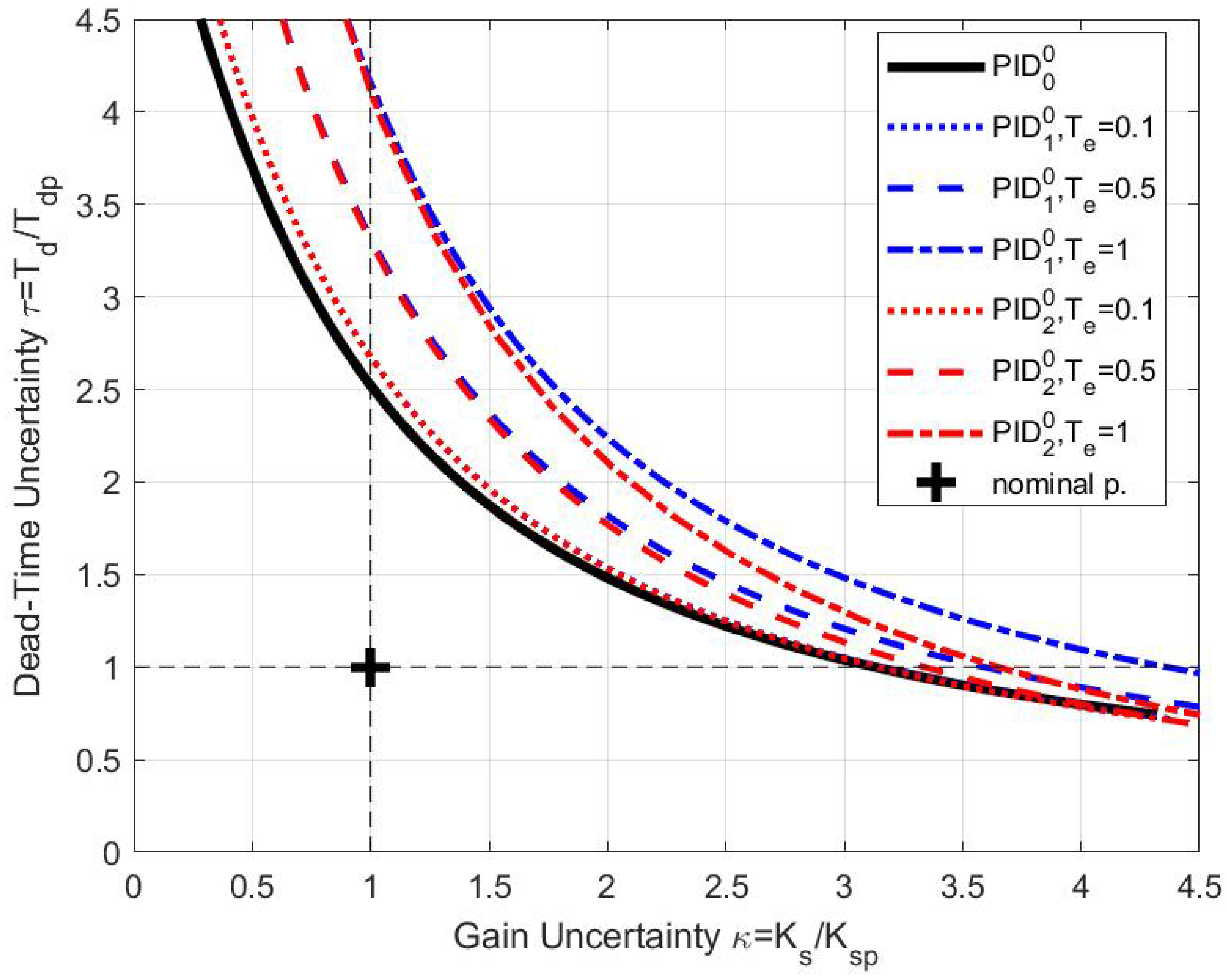
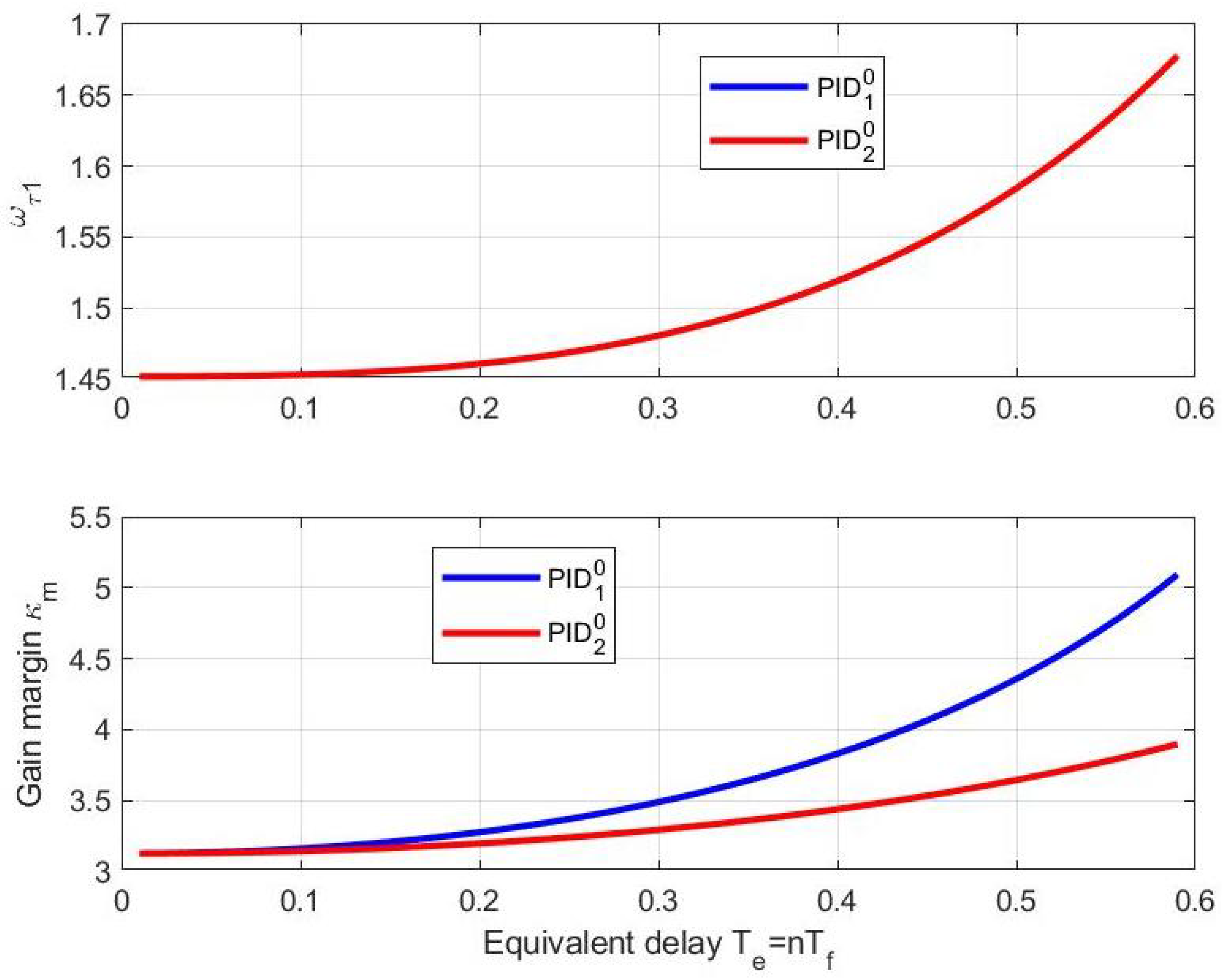
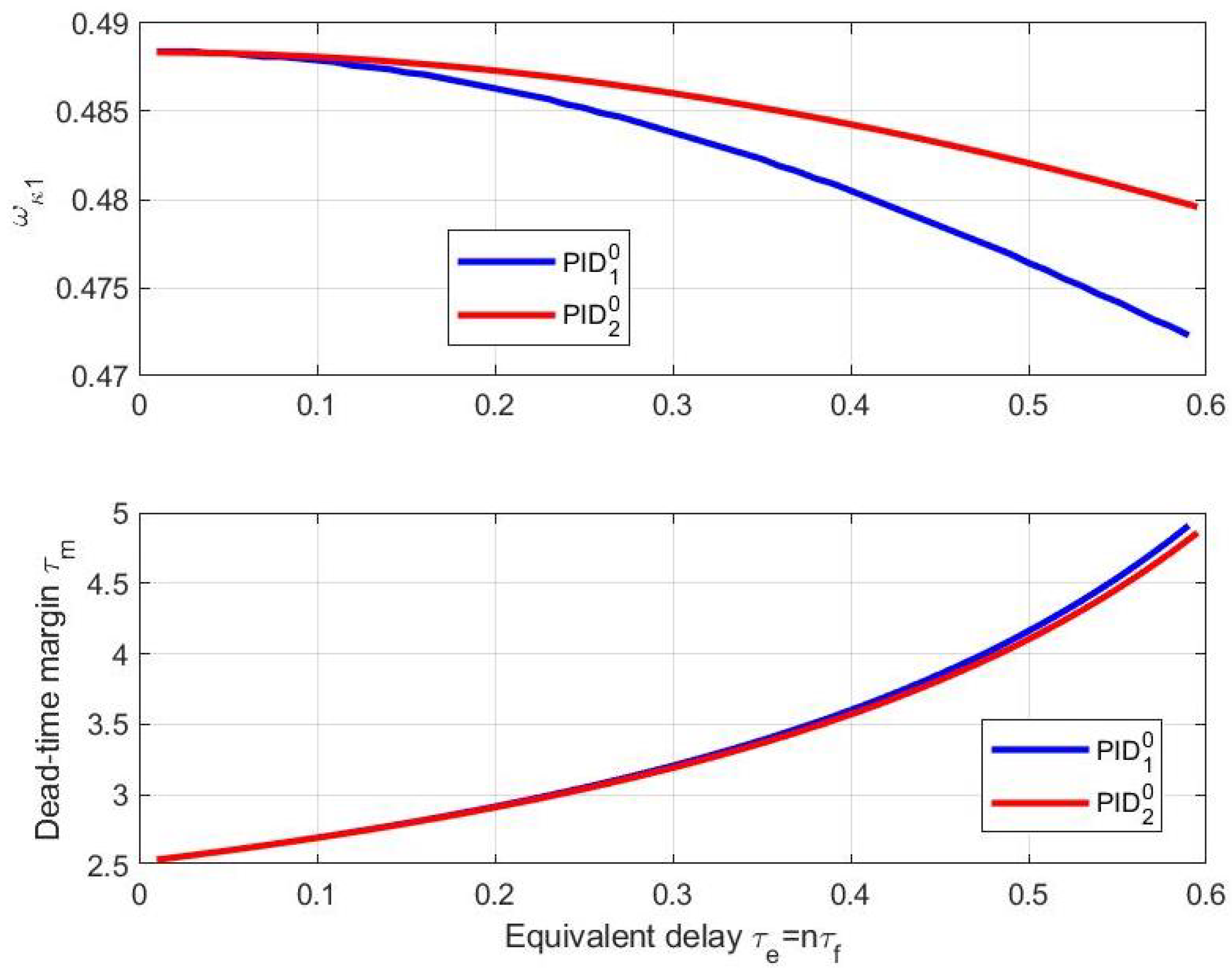
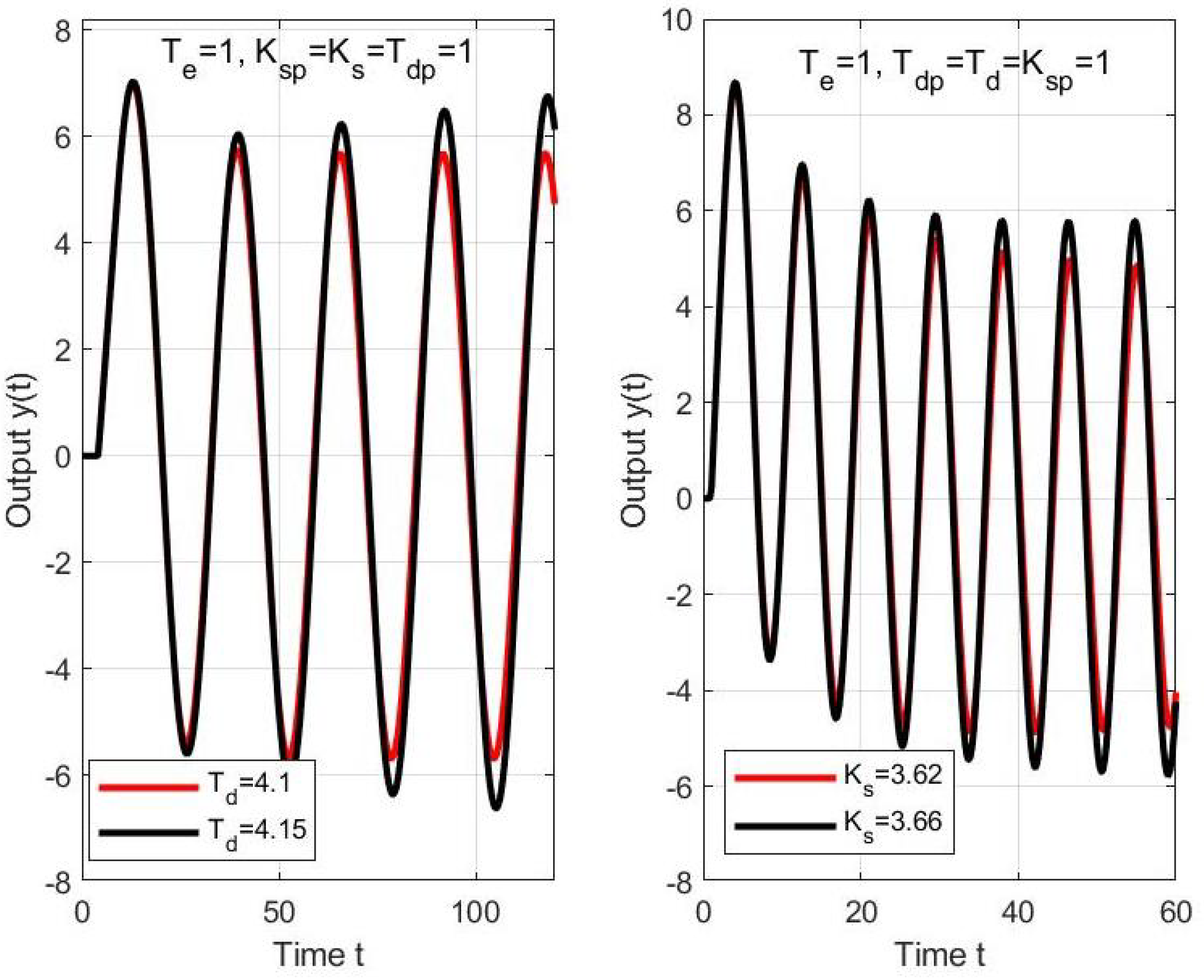
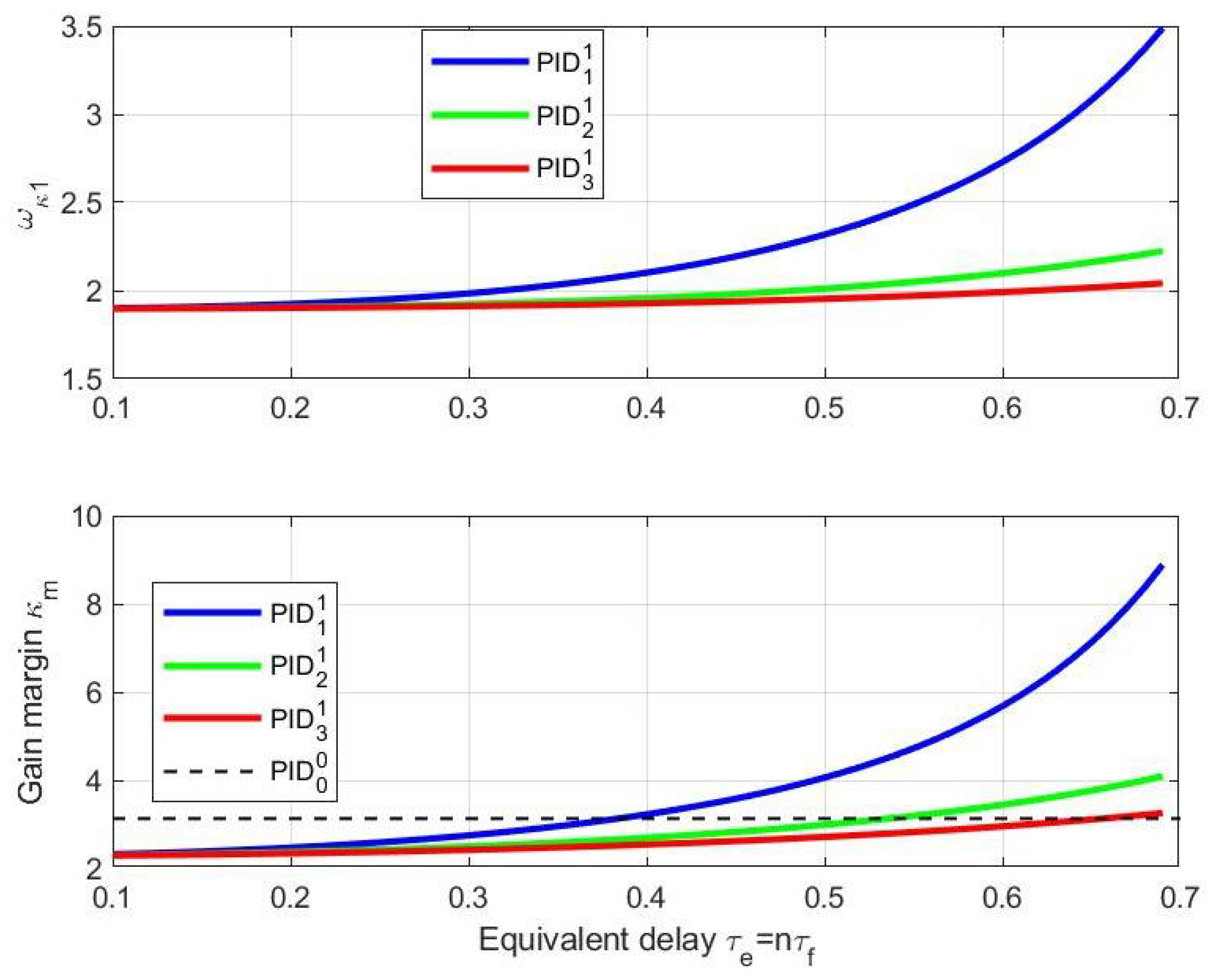
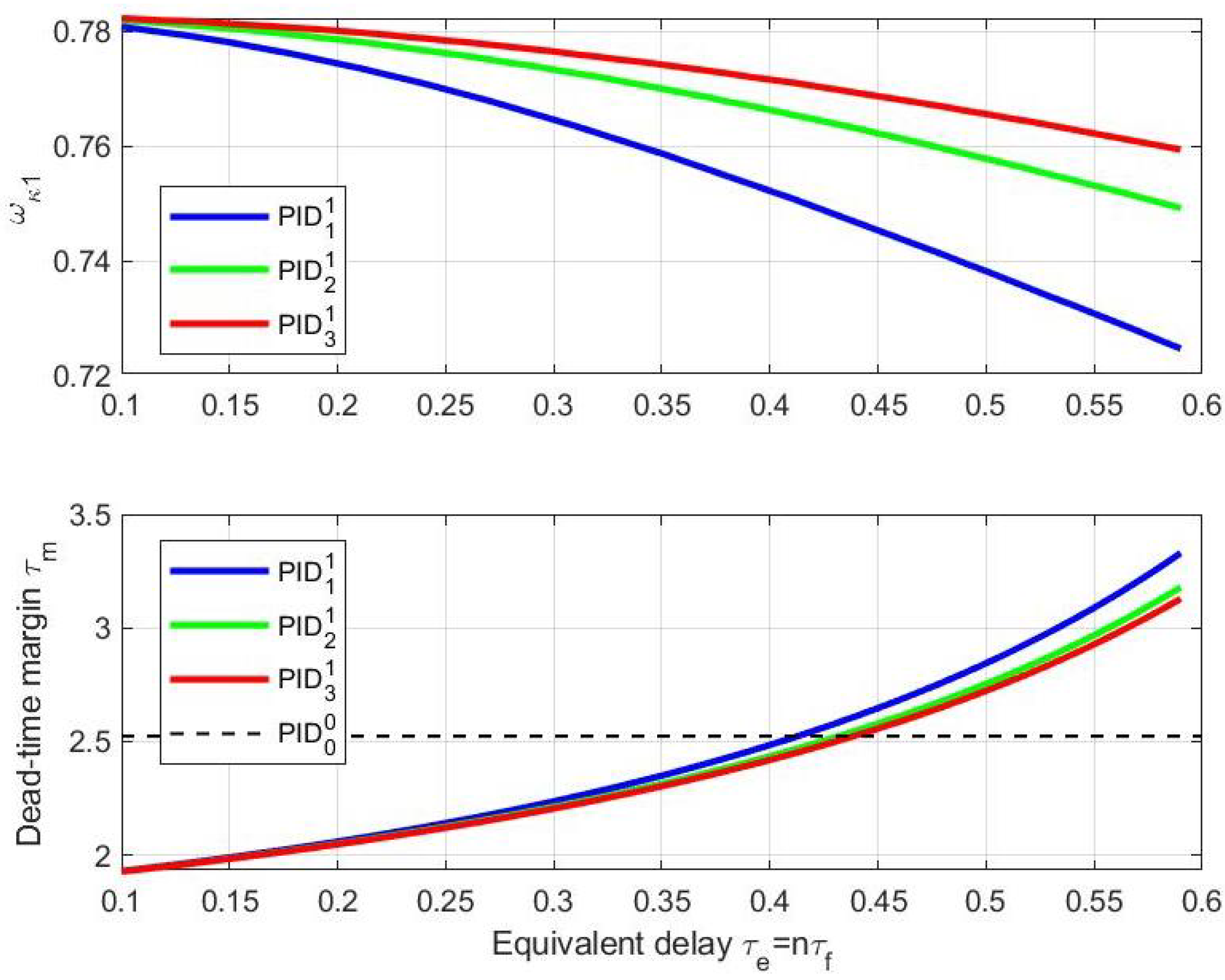
5. Robust Stability of Filtered PID Control

While the low-pass filter is optional for PI controllers, it is already necessary for PID controllers and can significantly reduce the resulting performance if the chosen filter is inappropriate. This is one of the reasons for the lower application of PID controllers compared to PI controllers.

For the nth-order filters, the characteristic polynomial corresponding to the controller designated as $PI{D}_n^1$ is

$$\begin{array}{c}P(j\Omega )=-T_i{\Omega }^2{(1+j\Omega T_f)}^n{e}^{j\Omega T_d}+K_c{K}_s[1+j\Omega T_i(1+j\Omega T_{D1})]\hfill \end{array}$$

(46)

For the nominal case, the controller parameters are given in Tab. Table 1 and

$$\begin{array}{c}{T}_d=T_{dp}+T_e;K_c={\displaystyle \frac{K_o}{K_{sp}(T_{dp}+T_e)}};\hfill \\ T_i={\tau }_i(T_{dp}+T_e);T_{D1}={\tau }_1(T_{dp}+T_e);\hfill \\ {\tau }_i=3.73204;K=0.78361;{\tau }_1=0.2628.\hfill \end{array}$$

(47)

For stability analysis, it is more convenient to work with dimensionless variables (16), when the system at the stability boundary is described by the following complex quasi-polynomial

$$\begin{array}{c}P\left(j\omega \right)=-{\tau }_i{\omega }^2{(1+j\omega {\tau }_f)}^n{e}^{j\omega \overline{\tau }}+\kappa K[1+j\omega {\tau }_i(1+j\omega {\tau }_1)]\hfill \end{array}$$

(48)

To determine the critical controller parameters, Equation (48) can be transformed into the equation with absolute values

$${\tau }_i{\omega }^2{\left(\sqrt{1+{\omega }^2{\tau }_f^2}\right)}^n=\kappa K\sqrt{{(1-{\omega }^2{\tau }_i{\tau }_D)}^2+{\omega }^2{\tau }_i^2}$$

(49)

or in two equations for real and imaginary parts. Again, the investigation is divided according to the chosen filter order n.

5.1. PID with the First-Order Filters

For $n=1$, two real equations can be formulated on the basis of (48)

$$\begin{array}{c}-{\tau }_i{\omega }^2[cos\left(\omega \overline{\tau }\right)-\omega {\tau }_{f}sin\left(\omega \overline{\tau }\right)]+\kappa K(1-{\omega }^2{\tau }_i{\tau }_D)=0\hfill \\ -{\tau }_i{\omega }^2[sin\left(\omega \overline{\tau }\right)+\omega {\tau }_{f}cos\left(\omega \overline{\tau }\right)]+\kappa K\omega {\tau }_i=0\hfill \end{array}$$

(50)

For $\omega =0$, according to the first equation, the stability limit is $\kappa =0$ (20).

Eliminating $\kappa K$ from Equation (50), we obtain for $\omega >0$ the equation

$${\displaystyle \frac{cos\left(\omega \overline{\tau }\right)-\omega {\tau }_{f}sin\left(\omega \overline{\tau }\right)}{1-{\omega }^2{\tau }_i{\tau }_D}}=\frac{sin\left(\omega \overline{\tau }\right)+\omega {\tau }_{f}cos\left(\omega \overline{\tau }\right)}{\omega {\tau }_i},$$

(51)

from which we finally obtain

$$\tau ={\displaystyle \frac{1+{\displaystyle \frac{{\tau }_e}{1-{\tau }_e}}}{\omega }}arctg\left(\omega {\displaystyle \frac{{\tau }_i-(1-{\tau }_i{\tau }_D{\omega }^2){\tau }_f}{1+{\omega }^2({\tau }_i{\tau }_f-{\tau }_i{\tau }_D)}}\right).$$

(52)

Considering (49) and $n=1$, it is possible to plot the curves corresponding to the robust stability border in Figure 6. The segments of the stability border corresponding to $PI{D}_1^1$ have the boundary points

$$\begin{array}{c}B{P}_{10}^1={\displaystyle \frac{{\tau }_i-{\tau }_f}{1-{\tau }_e}}={\displaystyle \frac{{\tau }_i-{\tau }_e}{1-{\tau }_e}}\mathrm{for}\omega \to 0\hfill \\ B{P}_{1\infty }^1=(\infty ,0)\mathrm{for}\omega \to \infty .\hfill \end{array}$$

(53)

5.2. PID with the Second-Order Filter

For $n=2$, two equations can be formulated based on (48)

$$\begin{array}{c}-{\tau }_i{\omega }^2[(1-{\omega }^2{\tau }_f^2)cos\left(\omega \overline{\tau }\right)-2\omega {\tau }_{f}sin\left(\omega \overline{\tau }\right)]+\kappa K(1-{\omega }^2{\tau }_i{\tau }_D)=0\hfill \\ -{\tau }_i{\omega }^2[(1-{\omega }^2{\tau }_f^2)sin\left(\omega \overline{\tau }\right)+2\omega {\tau }_{f}cos\left(\omega \overline{\tau }\right)]+\kappa K\omega {\tau }_i=0\hfill \end{array}$$

(54)

For $\omega =0$, it follows from the first equation that the stability limit is defined by the critical line $\kappa =0$ (20).

Eliminating $\kappa K$ from (50), for $\omega >0$ we obtain

$$\begin{array}{c}{\displaystyle \frac{(1-{\omega }^2{\tau }_f^2)cos\left(\omega \overline{\tau }\right)-2\omega {\tau }_{f}sin\left(\omega \overline{\tau }\right)}{1-{\omega }^2{\tau }_i{\tau }_D}}=\hfill \\ ={\displaystyle \frac{(1-{\omega }^2{\tau }_f^2)sin\left(\omega \overline{\tau }\right)+2\omega {\tau }_{f}cos\left(\omega \overline{\tau }\right)}{\omega {\tau }_i}},\hfill \end{array}$$

(55)

from which we finally get

$$\tau ={\displaystyle \frac{1+{\displaystyle \frac{{\tau }_e}{1-{\tau }_e}}}{\omega }}arctg\frac{(1-{\omega }^2{\tau }_f^2)\omega {\tau }_i-2\omega {\tau }_f(1-{\omega }^2{\tau }_i{\tau }_D)}{(1-{\omega }^2{\tau }_f^2)\omega {\tau }_i+2{\omega }^2{\tau }_i{\tau }_f}.$$

(56)

The stability boundary segments corresponding to $PI{D}_2^1$ have the boundary points

$$\begin{array}{c}B{P}_{20}^1={\displaystyle \frac{{\tau }_i-2{\tau }_f}{1-{\tau }_e}}={\displaystyle \frac{{\tau }_i-{\tau }_e}{1-{\tau }_e}}\mathrm{for}\omega \to 0\hfill \\ B{P}_{2\infty }^1=(\infty ,0)\mathrm{for}\omega \to \infty .\hfill \end{array}$$

(57)

Considering (49) and $n=2$, it is then possible to draw curves corresponding to the robust stability border in Figure 6.

5.3. PID with the Third-Order Filter

For $n=3$, the following two equations can be formulated based on (48)

$$\begin{array}{c}-{\tau }_i{\omega }^2[(1-3{\omega }^2{\tau }_f^2)cos\left(\omega \overline{\tau }\right)-\omega {\tau }_f(3-{\omega }^2{\tau }_f^2)sin\left(\omega \overline{\tau }\right)]+\kappa K(1-{\omega }^2{\tau }_i{\tau }_D)=0\hfill \\ -{\tau }_i{\omega }^2[(1-3{\omega }^2{\tau }_f^2)sin\left(\omega \overline{\tau }\right)+\omega {\tau }_f(3-{\omega }^2{\tau }_f^2)cos\left(\omega \overline{\tau }\right)]+\kappa K\omega {\tau }_i=0\hfill \end{array}$$

(58)

For $\omega =0$, the stability limit according to the first equation is again the critical line $\kappa =0$ (20).

Eliminating $\kappa K$ from Equation (50), we obtain for $\omega >0$ the equation

$$\begin{array}{c}{\displaystyle \frac{(1-3{\omega }^2{\tau }_f^2)cos\left(\omega \overline{\tau }\right)-\omega {\tau }_f(3-{\omega }^2{\tau }_f^2)sin\left(\omega \overline{\tau }\right)}{1-{\omega }^2{\tau }_i{\tau }_D}}=\hfill \\ ={\displaystyle \frac{(1-3{\omega }^2{\tau }_f^2)sin\left(\omega \overline{\tau }\right)+\omega {\tau }_f(3-{\omega }^2{\tau }_f^2)cos\left(\omega \overline{\tau }\right)}{\omega {\tau }_i}},\hfill \end{array}$$

(59)

from which we finally get

$$\begin{array}{c}\overline{\tau }={\displaystyle \frac{1}{\omega }}arctg{\displaystyle \frac{(1-3{\omega }^2{\tau }_f^2)\omega {\tau }_i-\omega {\tau }_f(3-{\omega }^2{\tau }_f^2)(1-{\omega }^2{\tau }_i{\tau }_D)}{(1-3{\omega }^2{\tau }_f^2)(1-{\omega }^2{\tau }_i{\tau }_D)+\omega {\tau }_f(3-{\omega }^2{\tau }_f^2)\omega {\tau }_i}},\hfill \\ \tau =(1+{\displaystyle \frac{{\tau }_e}{1-{\tau }_e}})\overline{\tau }.\hfill \end{array}$$

(60)

Combining (49) and $n=3$, it is then possible to draw the curves corresponding to the robust stability border in Figure 6.

The segments of the stability border corresponding to $PI{D}_3^1$ have the following boundary points

$$\begin{array}{c}B{P}_{30}^1={\displaystyle \frac{{\tau }_i-3{\tau }_f}{1-{\tau }_e}}={\displaystyle \frac{{\tau }_i-{\tau }_e}{1-{\tau }_e}}\mathrm{for}\omega \to 0\hfill \\ B{P}_{3\infty }^1=(\infty ,0)\mathrm{for}\omega \to \infty .\hfill \end{array}$$

(61)

5.4. Discussion about Filtered PID Control

For all values n considered, it may be interesting to study the stability boundary points $B{P}_{n\kappa }^1=({\kappa }_m,1)$ and $B{P}_{n\tau }^1=(1,{\tau }_m)$ that define the dead-time margins and the gain margins.

The dependence of the dead-time and the gain margins on ${\tau }_e=T_e/(T_{dp}+T_e)$ and the comparison of the two considered filter options are shown in Figure 7 and Figure 8.

When using the PID control with $T_e<Tdp$ (${\tau }_e<0.5$), the performed analysis shows a slight deterioration of the robust stability compared to PI without filtering. For small values of $\kappa =K_s/K_{sp}$ when $T_e=n{T}_f$ is applied, the robust stability practically does not depend on the filter order n. For higher values of $\kappa$, the stability decreases with increasing filter order n. It is, therefore, reasonable to choose a model identification method that yields the largest possible absolute estimate of $K_{sp}$.

The asymmetry of robust stability with respect to the uncertainties of the individual model parameters and the filter degrees n used is also evident in the calculation of the gain and dead-time margins ${\kappa }_m$ and ${\tau }_m$ (see Figure 7 and Figure 8). For the dead-time margin ${\tau }_m$, stability is almost not dependent on n, and improvements over the unfiltered PI control can be approximately achieved for $t_e\ge 0.4$. However, for $n=3$ and $T_e=n{T}_f$, the gain margin ${\kappa }_m=3.129$ of the unfiltered PI control (30) is achieved at ${\tau }_e\approx 0.66$, which is nearly twice as long as ${\tau }_e\approx 0.38$ for $n=1$. Thus, the suitability of using higher-order filters cannot be affirmed or rejected in a blanket manner but depends on the specific application.

Let us note that all considered boundary points $B_{n0}^m,m=0,1$ are formally given by the same relation. If we assign the index m to the considered values ${\tau }_i$ and ${\tau }_e$ and search for a value for ${\tau }_e^1$ that leads to a dynamics corresponding to the unfiltered PI ($PI{D}_0^0$) with ${\tau }_e^0=0$, we have to solve the following equation

$${\displaystyle \frac{{\tau }_i^0-{\tau }_e^0}{1-{\tau }_e^0}}={\displaystyle \frac{{\tau }_i^1-{\tau }_e^1}{1-{\tau }_e^1}}$$

(62)

This gives

$${\tau }_e^1={\displaystyle \frac{{\tau }_i^0-{\tau }_i^1}{{\tau }_i^0-1}}=0.4342$$

(63)

This result is in good agreement with the graphical solution of the equivalence based on the dead-time span curves in Figure 8.

Similarly, it would be possible to estimate the values of ${\tau }_e$ that ensure the equivalence of the filtered PID controller with the filtered PI controller.

The use of one or more derived terms should also be justified in terms of robustness. For the chosen value of the parameter ${\tau }_e$, which provides at least the same gain and stability margins as the unfiltered PI, in the nominal case with exactly known parameters of the model, we obtain the input and output responses of the closed loop as shown in Figure 9. The maximum amplitudes of the disturbance responses at the input and output of the process can also be higher than for unfiltered PI. This is due to the fact that adding $T_e$ to the process delay $T_{dp}$ increases the total delay. Therefore, after a disturbance step, the maximum deviations at the input and output of the system increase.

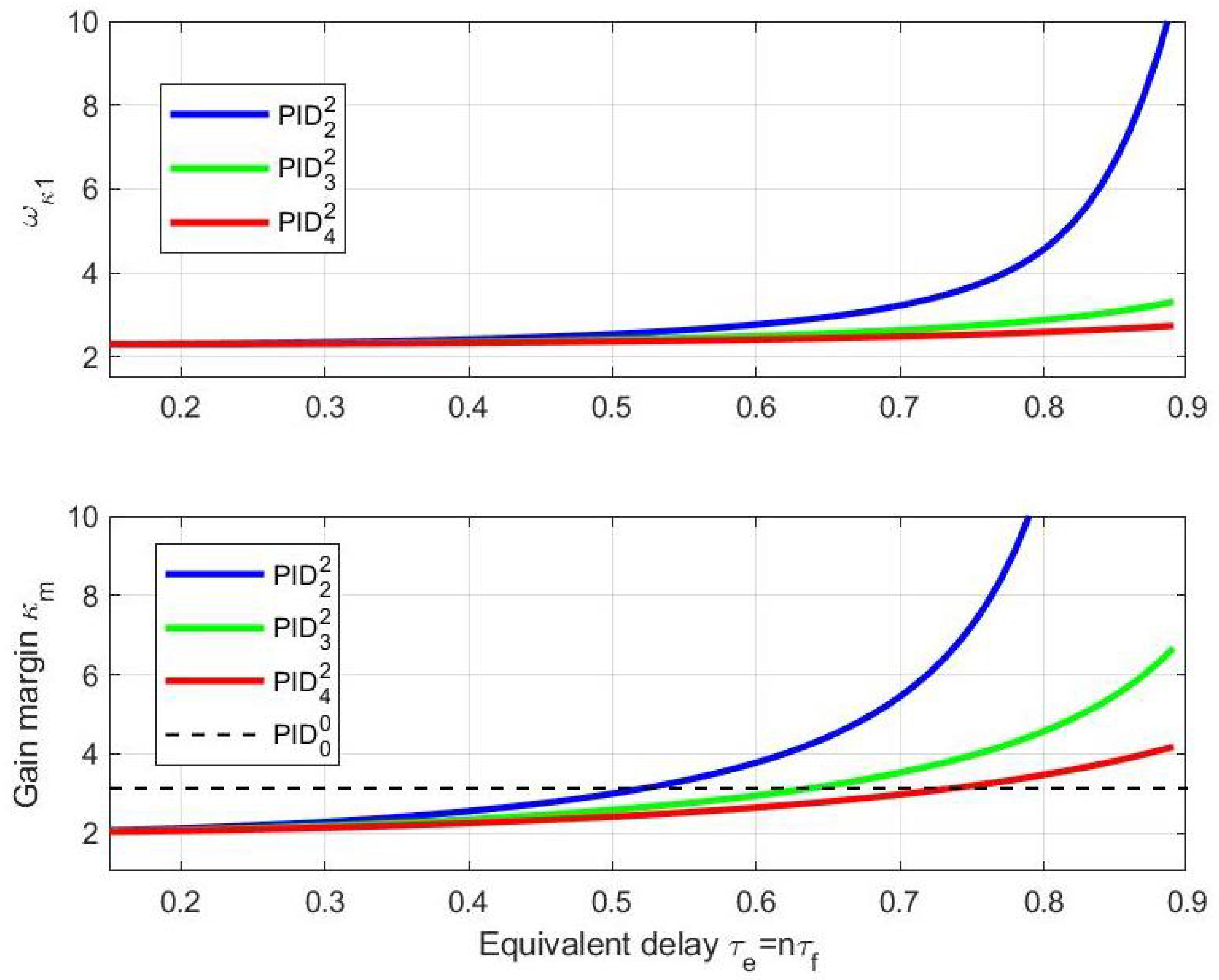
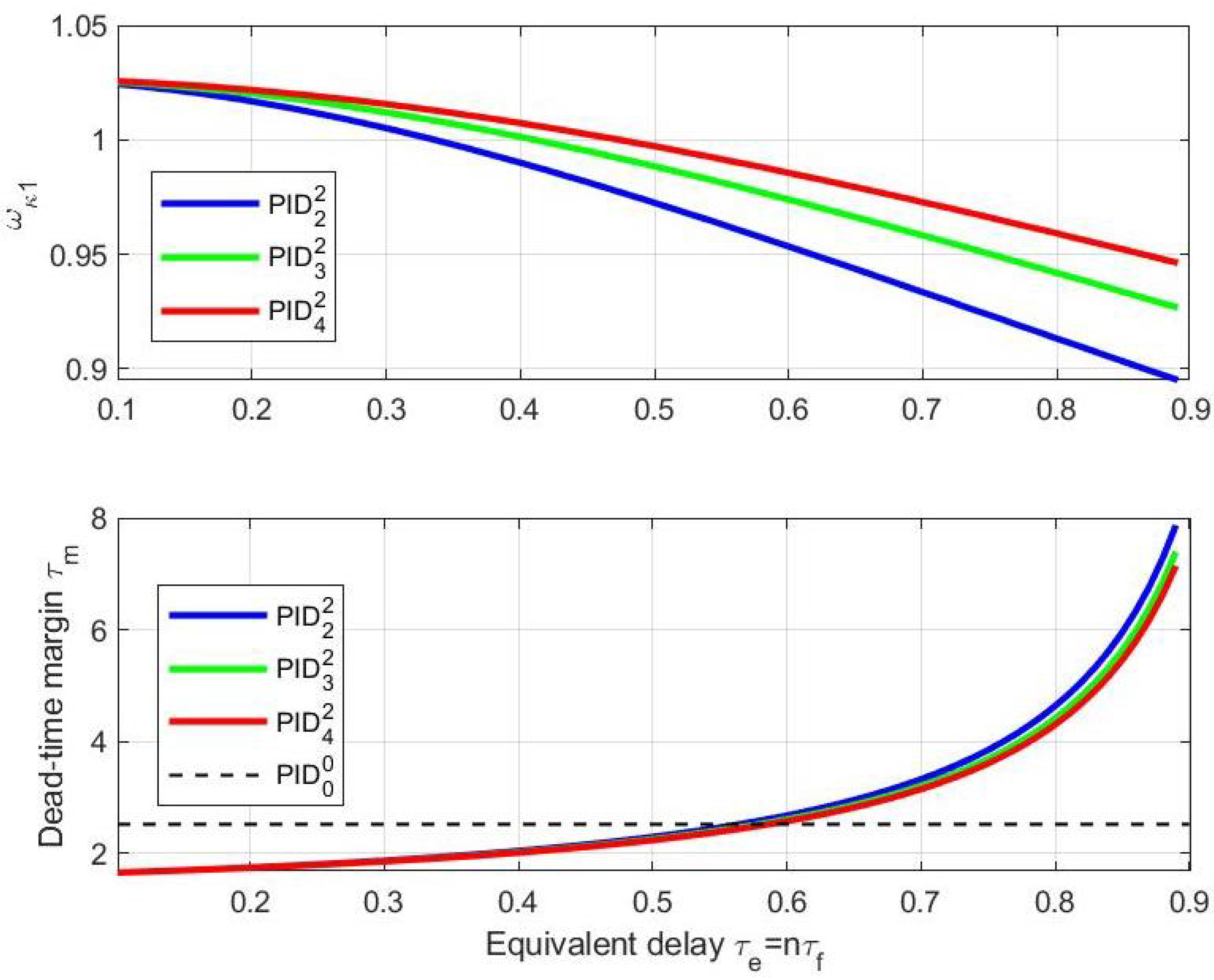
6. Robust Stability of PIDA Controller

Similar to the PID controller, the implementation of the PIDA controller requires at least a 2nd order filter. For the nth-order filters, the characteristic polynomial corresponding to the controller denoted as $PI{D}_n^2$ is

$$\begin{array}{c}P(j\Omega )=-T_i{\Omega }^2{(1+j\Omega T_f)}^n{e}^{j\Omega T_d}+K_c{K}_s[1+j\Omega T_i(1+j\Omega T_{D1}-{\Omega }^2{T}_{D2}^2)]\hfill \end{array}$$

(64)

For the nominal case, the controller parameters are given in Table 1 and

$$\begin{array}{c}{T}_d=T_{dp}+T_e;K_c={\displaystyle \frac{K}{K_{sp}(T_{dp}+T_e)}};\hfill \\ T_i={\tau }_i(T_{dp}+T_e);T_{D1}={\tau }_1(T_{dp}+T_e);T_{D2}^2={\tau }_2{(T_{dp}+T_e)}^2;\hfill \\ {\tau }_i=3.0;K=1.08268;{\tau }_1=0.37500;{\tau }_2=0.04167.\hfill \end{array}$$

(65)

For stability analysis, it is more convenient to work with dimensionless variables (16), when the system at the stability limit is described by the complex quasi-polynomial

$$\begin{array}{c}P\left(j\omega \right)=-{\tau }_i{\omega }^2{(1+j\omega {\tau }_f)}^n{e}^{j\omega \overline{\tau }}+\kappa K[1+j\omega {\tau }_i(1-{\omega }^2{\tau }_2+j\omega {\tau }_1)]\hfill \end{array}$$

(66)

When determining the critical controller tuning, it can be converted into the equation with absolute values

$${\tau }_i{\omega }^2{\left(\sqrt{1+{\omega }^2{\tau }_f^2}\right)}^n=\kappa K\sqrt{{(1-{\omega }^2{\tau }_i{\tau }_1)}^2+{\omega }^2{\tau }_i^2{(1-{\omega }^2{\tau }_2)}^2}$$

(67)

or in two equations for real and imaginary parts. Again, we will treat the conditions for the different orders n separately.

6.1. PIDA with the Second-Order Filters

For $n=2$, the following two equations can be formulated based on (48):

$$\begin{array}{c}-{\tau }_i{\omega }^2[(1-{\omega }^2{\tau }_f^2)cos\left(\omega \overline{\tau }\right)-2\omega {\tau }_{f}sin\left(\omega \overline{\tau }\right)]+\kappa K(1-{\omega }^2{\tau }_i{\tau }_1)=0\hfill \\ -{\tau }_i{\omega }^2[(1-{\omega }^2{\tau }_f^2)sin\left(\omega \overline{\tau }\right)+2\omega {\tau }_{f}cos\left(\omega \overline{\tau }\right)]+\kappa K\omega {\tau }_i(1-{\omega }^2{\tau }_2)=0\hfill \end{array}$$

(68)

For $\omega =0$, the first equation provides the stability limit in the form of the critical line $\kappa =0$ (20).

Eliminating $\kappa K$ from Equation (68), we obtain (for $\omega >0$) the expression

$${\displaystyle \frac{(1-{\omega }^2{\tau }_f^2)cos\left(\omega \overline{\tau }\right)-2\omega {\tau }_{f}sin\left(\omega \overline{\tau }\right)}{1-{\omega }^2{\tau }_i{\tau }_1}}=\frac{(1-{\omega }^2{\tau }_f^2)sin\left(\omega \overline{\tau }\right)+2\omega {\tau }_{f}cos\left(\omega \overline{\tau }\right)}{\omega {\tau }_i(1-{\omega }^2{\tau }_2)},$$

(69)

from which we finally get

$$\tau ={\displaystyle \frac{1+{\displaystyle \frac{{\tau }_e}{1-{\tau }_e}}}{\omega }}arctg\left({\displaystyle \frac{\omega {\tau }_i(1-{\omega }^2{\tau }_2)(1-{\omega }^2{\tau }_f^2)-2\omega {\tau }_f(1-{\omega }^2{\tau }_i{\tau }_1)}{2\omega {\tau }_f{\tau }_i(1-{\omega }^2{\tau }_2)+(1-{\omega }^2{\tau }_2)(1-{\omega }^2{\tau }_i{\tau }_1)}}\right).$$

(70)

The stability boundary segments corresponding to $PI{D}_2^2$ have the boundary points

$$\begin{array}{c}B{P}_{20}^2={\displaystyle \frac{{\tau }_i-2{\tau }_f}{1-{\tau }_e}}={\displaystyle \frac{{\tau }_i-{\tau }_e}{1-{\tau }_e}}\mathrm{for}\omega \to 0\hfill \\ B{P}_{2\infty }^2=(\infty ,0)\mathrm{for}\omega \to \infty .\hfill \end{array}$$

(71)

In combination with (67), it is then possible to draw curves corresponding to the robust stability border in Figure 10.

6.2. PIDA with the Third-Order Filters

For $n=3$, two equations can be formulated based on (48)

$$\begin{array}{c}-{\tau }_i{\omega }^2[(1-3{\omega }^2{\tau }_f^2)cos\left(\omega \overline{\tau }\right)-\omega {\tau }_f(3-{\omega }^2{\tau }_f^2)sin\left(\omega \overline{\tau }\right)]+\kappa K(1-{\omega }^2{\tau }_i{\tau }_1)=0\hfill \\ -{\tau }_i{\omega }^2[(1-3{\omega }^2{\tau }_f^2)sin\left(\omega \overline{\tau }\right)+\omega {\tau }_f(3-{\omega }^2{\tau }_f^2)cos\left(\omega \overline{\tau }\right)]+\kappa K\omega {\tau }_i(1-{\omega }^2{\tau }_2)=0\hfill \end{array}$$

(72)

For $\omega =0$, the first equation provides the stability limit in terms of the critical line $\kappa =0$ (20).

Eliminating $\kappa K$ from Equation (72), for $\omega >0$ we obtain the equation

$$\begin{array}{c}{\displaystyle \frac{(1-3{\omega }^2{\tau }_f^2)cos\left(\omega \overline{\tau }\right)-\omega {\tau }_f(3-{\omega }^2{\tau }_f^2)sin\left(\omega \overline{\tau }\right)}{1-{\omega }^2{\tau }_i{\tau }_1}}=\hfill \\ ={\displaystyle \frac{(1-3{\omega }^2{\tau }_f^2)sin\left(\omega \overline{\tau }\right)+\omega {\tau }_f(3-{\omega }^2{\tau }_f^2)cos\left(\omega \overline{\tau }\right)}{\omega {\tau }_i(1-{\omega }^2{\tau }_2)}},\hfill \end{array}$$

(73)

from which we finally get

$$\tau ={\displaystyle \frac{1+{\displaystyle \frac{{\tau }_e}{1-{\tau }_e}}}{\omega }}arctg\left({\displaystyle \frac{\omega {\tau }_i(1-{\omega }^2{\tau }_2)(1-3{\omega }^2{\tau }_f^2)-\omega {\tau }_f(1-{\omega }^2{\tau }_i{\tau }_1)(3-{\omega }^2{\tau }_f^2)}{(1-3{\omega }^2{\tau }_f^2)(1-{\omega }^2{\tau }_i{\tau }_1)+{\omega }^2{\tau }_i{\tau }_f(1-{\omega }^2{\tau }_2)(3-{\omega }^2{\tau }_f^2)}}\right).$$

(74)

The stability boundary segments of $PI{D}_3^2$ have the boundary points

$$\begin{array}{c}B{P}_{30}^2={\displaystyle \frac{{\tau }_i-3{\tau }_f}{1-{\tau }_e}}={\displaystyle \frac{{\tau }_i-{\tau }_e}{1-{\tau }_e}}\mathrm{for}\omega \to 0\hfill \\ B{P}_{3\infty }^{2}1=(\infty ,0)\mathrm{for}\omega \to \infty .\hfill \end{array}$$

(75)

In combination with (67), it is then possible to draw curves corresponding to the robust stability border in Figure 10.

6.3. PIDA with the Fourth-Order Filters

For $n=4$, two equations can be formulated based on (48):

$$\begin{array}{c}-{\tau }_i{\omega }^2[(1-6{\omega }^2{\tau }_f^2+{\omega }^4{\tau }_f^4)cos\left(\omega \overline{\tau }\right)-4\omega {\tau }_f(1-{\omega }^2{\tau }_f^2)sin\left(\omega \overline{\tau }\right)]+\kappa K(1-{\omega }^2{\tau }_i{\tau }_1)=0\hfill \\ -{\tau }_i{\omega }^2[(1-6{\omega }^2{\tau }_f^2+{\omega }^4{\tau }_f^4)sin\left(\omega \overline{\tau }\right)+4\omega {\tau }_f(1-{\omega }^2{\tau }_f^2)cos\left(\omega \overline{\tau }\right)]+\kappa K\omega {\tau }_i(1-{\omega }^2{\tau }_2)=0\hfill \end{array}$$

(76)

For $\omega =0$, the first equation provides the stability limit in the form of the critical line $\kappa =0$ (20).

Eliminating $\kappa K$ from Equation (72), for $\omega >0$, we obtain

$$\begin{array}{c}{\displaystyle \frac{(1-6{\omega }^2{\tau }_f^2+{\omega }^4{\tau }_f^4)cos\left(\omega \overline{\tau }\right)-4\omega {\tau }_f(1-{\omega }^2{\tau }_f^2)sin\left(\omega \overline{\tau }\right)}{1-{\omega }^2{\tau }_i{\tau }_1}}=\hfill \\ ={\displaystyle \frac{(1-6{\omega }^2{\tau }_f^2+{\omega }^4{\tau }_f^4)sin\left(\omega \overline{\tau }\right)+4\omega {\tau }_f(1-{\omega }^2{\tau }_f^2)cos\left(\omega \overline{\tau }\right)}{\omega {\tau }_i(1-{\omega }^2{\tau }_2)}},\hfill \end{array}$$

(77)

from which we finally get

$$\tau ={\displaystyle \frac{1+{\displaystyle \frac{{\tau }_e}{1-{\tau }_e}}}{\omega }}arctg\left({\displaystyle \frac{(1-6{\omega }^2{\tau }_f^2+{\omega }^4{\tau }_f^4)\omega {\tau }_i(1-{\omega }^2{\tau }_2)-4\omega {\tau }_f(1-{\omega }^2{\tau }_f^2)(1-{\omega }^2{\tau }_i{\tau }_1)}{(1-6{\omega }^2{\tau }_f^2+{\omega }^4{\tau }_f^4)(1-{\omega }^2{\tau }_i{\tau }_1)+4{\omega }^2{\tau }_f{\tau }_i(1-{\omega }^2{\tau }_f^2)(1-{\omega }^2{\tau }_2)}}\right).$$

(78)

The stability boundary segments corresponding to $PI{D}_4^2$ have the boundary points

$$\begin{array}{c}B{P}_{40}^2={\displaystyle \frac{{\tau }_i-4{\tau }_f}{1-{\tau }_e}}={\displaystyle \frac{{\tau }_i-{\tau }_e}{1-{\tau }_e}}\mathrm{for}\omega \to 0\hfill \\ B{P}_{4\infty }^{2}1=(\infty ,0)\mathrm{for}\omega \to \infty .\hfill \end{array}$$

(79)

In combination with (67), it is then possible to draw curves corresponding to the robust stability border in Figure 10.

The dependence of the stability and gain margins on ${\tau }_e=T_e/(T_{dp}+T_e)$ and the comparison of the considered filtration options are shown in Figure 11 and Figure 12, respectively.

6.4. Discussion on the Filtered PIDA Control

The analysis of the robust stability of the PIDA controller allows to formulate similar conclusions as for the PID controller. When applying higher- order filters $n>2$, the $K_{sp}$ should be chosen so that the process is well approximated with variable (non-zero) gain $K_s$ at the highest determined absolute values of $K_s$.

Again, all boundary points $B_{n0}^2$ considered are formally given by the same relation as for $m=0$ or $m=1$. Therefore, for $m=2$ we can find ${\tau }_e^2$ leading to the dynamics corresponding to the unfiltered PI ($PI{D}_0^0$) with ${\tau }_e^0=0$. By solving the equation

$${\displaystyle \frac{{\tau }_i^0-{\tau }_e^0}{1-{\tau }_e^0}}={\displaystyle \frac{{\tau }_i^2-{\tau }_e^2}{1-{\tau }_e^2}}$$

(80)

one obtains

$${\tau }_e^2={\displaystyle \frac{{\tau }_i^0-{\tau }_i^2}{{\tau }_i^0-1}}=0.5858$$

(81)

This result is in good agreement with the graphical solution of the equivalence based on the $B_{n\tau }^2$ boundary points and the corresponding dead-time margin curves in Figure 12.

7. Conclusions

The evaluation of the stability range, which depends on the derivative term and the applied low-pass filters, showed that the filtering itself increases the robust stability of the control loop. When the uncertainty of $\kappa =K_s/K_{sp}$ is large, it is advisable to use low-pass filters with the minimal possible order. The possibility of using higher-order filters should already be taken into account when selecting the model parameter $K_{sp}$ during process identification to get $max\left\{\kappa \right\}\approx 1$.

If we want to speed up transient responses by including derivative components compared to an unfiltered PI controller and using more “aggressive” settings (choosing lower values of $T_e$), we must not be surprised by a decrease in the range of stable parameters, i.e. a decrease in robustness.

Simple analytical relations for setting filtered PI, PID, and PIDA controllers with equivalent robustness have been derived.

To ensure the operation of the circuit in the area of stability, even when considering the uncertainty of the model parameters, its nominal parameters must be appropriately selected.

In future research, we will focus on the evaluation of robust stability when higher-order derivative terms are used. The results obtained for $m=0,1$, and 2 indicate that they could also apply to higher values of m, which are interesting from the point of view of direct replacement of fractional-order PID controllers using approximations with higher-order filters.

References

- Visioli, A. Practical PID Control; Springer: London, UK, 2006. [Google Scholar]
- Åström, K.J.; Hägglund, T. Advanced PID Control; ISA, Research Triangle Park: Raleigh, NC, USA, 2006. [Google Scholar]
- Isaksson, A.; Graebe, S. Derivative filter is an integral part of PID design. Control Theory Appl. IEE Proc. 2002, 149, 41–45. [Google Scholar] [CrossRef]
- Ruel, P.E. Using filtering to improve performance. In Proceedings of the ISA Expo 2003, Houston, TX, USA, 21–23 October 2003. [Google Scholar]
- Hägglund, T. Signal Filtering in PID Control. IFAC Proc. Vol. 2012, 45, 1–10. [Google Scholar] [CrossRef] [Green Version]
- Micic, A.D.; Matausek, M.R. Optimization of PID controller with higher-order noise filter. J. Process Control 2014, 24, 694–700. [Google Scholar] [CrossRef]
- Segovia, V.R.; Hägglund, T.; Åström, K. Measurement noise filtering for PID controllers. J. Process Control 2014, 24, 299–313. [Google Scholar] [CrossRef]
- Fišer, J.; Zítek, P.; Vyhlídal, T. Dominant four-pole placement in filtered PID control loop with delay. IFAC-PapersOnLine 2017, 50, 6501–6506. [Google Scholar] [CrossRef]
- Peker, F.; Kaya, I. Optimal integral-proportional derivative controller design for input load disturbance rejection of time delay integrating processes. Proc. Inst. Mech. Eng. Part I J. Syst. Control Eng. 2022; in press. [Google Scholar]
- Huba, M. Filter choice for an effective measurement noise attenuation in PI and PID controllers. In Proceedings of the ICM2015, Casablanca, Morocco, 20–23 December 2015. [Google Scholar]
- Huba, M.; Bisták, P.; Huba, T. Filtered PI and PID control of an Arduino based thermal plant. IFAC-PapersOnLine 2016, 49, 336–341. [Google Scholar] [CrossRef]
- Majhi, S.; Kotwal, V.; Mehta, U. FPAA-Based PI controller for DC servo position control system. IFAC Proc. Vol. 2012, 45, 247–251. [Google Scholar] [CrossRef] [Green Version]
- Hasler, J. Large-Scale Field-Programmable Analog Arrays. Proc. IEEE 2020, 108, 1283–1302. [Google Scholar] [CrossRef]
- Valele, W.; Virambath, R.; Mehta, U.; Azid, S. Fractional analog scheme for efficient stabilization of a synchronous buck converter. J. Electr. Eng. 2020, 71, 116–121. [Google Scholar] [CrossRef]
- Huba, M.; Vrančić, D.; Bisták, P. PID Control with Higher Order Derivative Degrees for IPDT Plant Models. IEEE Access 2021, 9, 2478–2495. [Google Scholar] [CrossRef]
- Vrančić, D.; Huba, M. High-Order Filtered PID Controller Tuning Based on Magnitude Optimum. Mathematics 2021, 9, 1340. [Google Scholar] [CrossRef]
- Oldenbourg, R.; Sartorius, H. Dynamik Selbsttätiger Regelungen; R.Oldenbourg-Verlag: München, Germany, 1944. [Google Scholar]
- Vítečková, M.; Víteček, A. Two-degree of Freedom Controller Tuning for Integral Plus Time Delay Plants. ICIC Express Lett. Int. J. Res. Surv. Jpn. 2008, 2, 225–229. [Google Scholar]
- Vítečková, M.; Víteček, A. 2DOF PI and PID controllers tuning. In Proceedings of the 9th IFAC Workshop on Time Delay Systems, Guangzhou, China, 29 September–1 October 2010; Volume 9, pp. 343–348. [Google Scholar]
- Vítečková, M.; Víteček, A. 2DOF PID controller tuning for integrating plants. In Proceedings of the 2016 17th Int. Carpathian Control Conf. (ICCC), High Tatras, Slovakia, 29 May–1 June 2016; pp. 793–797. [Google Scholar]
- Víteček, A.; Vítečková, M. Series Two Degree of Freedom PID Controller for Integrating Plants with Time Delay. In Proceedings of the 2019 20th International Carpathian Control Conference (ICCC), Kraków-Wieliczka, Poland, 26–29 May 2019; pp. 1–4. [Google Scholar]
- Vítečková, M.; Víteček, A.; Janáčová, D. Robustness and Muliple Dominant Pole Method. In Proceedings of the 2020 21th ICCC, High Tatras, Slovakia, 27–29 October 2020; pp. 1–4. [Google Scholar]
- Huba, M. Designing Robust Controller Tuning for Dead Time Systems. In Int. Conf. System Structure and Control; IFAC: Ancona, Italy, 2010. [Google Scholar]
- Huba, M. Performance measures, performance limits and optimal PI control for the IPDT plant. J. Process Control 2013, 23, 500–515. [Google Scholar] [CrossRef]
- Huba, M. Comparing 2DOF PI and Predictive Disturbance Observer Based Filtered PI Control. J. Process Control 2013, 23, 1379–1400. [Google Scholar] [CrossRef]
- Oaxaca-Adams, G.; Villafuerte-Segura, R.; Aguirre-Hernández, B. On non-fragility of controllers for time delay systems: A numerical approach. J. Frankl. Inst. 2021, 358, 4671–4686. [Google Scholar] [CrossRef]
- Oaxaca-Adams, G.; Villafuerte-Segura, R. On controllers performance for a class of time-delay systems: Maximum decay rate. Automatica 2023, 147, 110669. [Google Scholar] [CrossRef]
- Huba, M.; Chamraz, S.; Bisták, P.; Vrančić, D. Making the PI and PID Controller Tuning Inspired by Ziegler and Nichols Precise and Reliable. Sensors 2021, 18, 6157. [Google Scholar] [CrossRef] [PubMed]
- Huba, M.; Gao, Z. Uncovering Disturbance Observer and Ultra-Local Plant Models in Series PI Controllers. Symmetry 2022, 14, 640. [Google Scholar] [CrossRef]
- Huba, M. Disturbance Observer in PID Controllers for First-Order Time-Delayed Systems. In Proceedings of the 13th IFAC Symposium Advances in Control Education, Hamburg, Germany, 24–27 July 2022. [Google Scholar]
- Huba, M.; Bisták, P. Should we forget the PID control? In Proceedings of the 2022 20th International Conference on Emerging eLearning Technologies and Applications (ICETA), High Tatras, Slovakia, 20–21 October 2022. [Google Scholar]
- Huba, M.; Vrančić, D. Comparing filtered PI, PID and PIDD2 control for the FOTD plants. In Proceedings of the 3rd IFAC Conference on Advances in Proportional-Integral-Derivative Control, Ghent, Belgium, 9–11 May 2018; pp. 954–959. [Google Scholar]
- Huba, M.; Vrančić, D. Introduction to the Discrete Time PID Control for the IPDT Plant. In Proceedings of the 15th IFAC Int. Conference on Programmable Devices and Embedded Systems, Ostrava, Czech Republic, 23–25 May 2018; pp. 119–124. [Google Scholar]
- Tepljakov, A.; Alagoz, B.B.; Yeroglu, C.; Gonzalez, E.; HosseinNia, S.H.; Petlenkov, E. FOPID Controllers and Their Industrial Applications: A Survey of Recent Results. IFAC-PapersOnLine 2018, 51, 25–30. [Google Scholar] [CrossRef]
- Huba, M.; Vrančić, D.; Bisták, P. PID Control for IPDT Plants. Part 1: Disturbance Response. In Proceedings of the 26th Mediterranean Conference on Control and Automation (MED), Zadar, Croatia, 19–22 June 2018. [Google Scholar]
- Huba, M. Performance Measures and the Robust and Optimal Control Design. In Proceedings of the 3rd IFAC Conference on Advances in Proportional-Integral-Derivative Control, Ghent, Belgium, 9–11 May 2018; pp. 960–965. [Google Scholar]
- Huba, M.; Vrančić, D. Extending the Model-Based Controller Design to Higher-Order Plant Models and Measurement Noise. Symmetry 2021, 2021, 798. [Google Scholar] [CrossRef]
- Huba, M.; Vrančić, D. Tuning of PID Control for the Double Integrator Plus Dead-Time Model by Modified Real Dominant Pole and Performance Portrait Methods. Mathematics 2022, 10, 971. [Google Scholar] [CrossRef]
- Fortuna, L.; Frasca, M. Optimal and Robust Control: Advanced Topics with MATLAB, 1st ed.; CRC Press: Boca Raton, FL, USA, 2012. [Google Scholar]
- Ackermann, J. Robust Control: The Parameter Space Approach, 2nd ed.; Springer: Berlin, Germany, 2002. [Google Scholar]
- Zítek, P.; Fišer, J.; Vyhlídal, T. Dimensional analysis approach to dominant three-pole placement in delayed PID control loops. J. Process Control 2013, 23, 1063–1074. [Google Scholar] [CrossRef]
- Huba, M.; Oliveira, P.M.; Bisták, P.; Vrančić, D. A Set of Active Disturbance Rejection Controllers Based on Integrator Plus Dead-Time Models. Appl. Sci. 2021, 2021, 1671. [Google Scholar] [CrossRef]
- Ferrari, M.; Visioli, A. A software tool to understand the design of PIDA controllers. IFAC-PapersOnLine 2022, 55, 249–254. [Google Scholar] [CrossRef]
- Visioli, A.; Sánchez-Moreno, J. A relay-feedback automatic tuning methodology of PIDA controllers for high-order processes. Int. J. Control, 2022; in press. [Google Scholar]
- Huba, M.; Vrančić, D. Delay Equivalences in Tuning PID Control for the Double Integrator Plus Dead-Time. Mathematics 2021, 9, 328. [Google Scholar] [CrossRef]
- Ziegler, J.G.; Nichols, N.B. Optimum settings for automatic controllers. Trans. ASME 1942, 64, 759–768. [Google Scholar] [CrossRef]
- Fliess, M.; Join, C. Model-free control. Int. J. Control 2013, 86, 2228–2252. [Google Scholar] [CrossRef] [Green Version]
- Gao, Z. On the centrality of disturbance rejection in automatic control. ISA Trans. 2014, 53, 850–857. [Google Scholar] [CrossRef] [Green Version]
- Mercader, P.; Banos, A. A PI tuning rule for integrating plus dead time processes with parametric uncertainty. ISA Trans. 2017, 67, 246–255. [Google Scholar] [CrossRef]
- Huba, M.; Bélai, I. Limits of a Simplified Controller Design Based on IPDT models. ProcIMechE Part I J. Syst. Control Eng. 2018, 232, 728–741. [Google Scholar] [CrossRef]
- Neimark, J.I. D-decomposition of the space of quasi-polynomials (on the stability of linearized distributive systems. Am. Math. Soc. Transl. 1973, 102, 95–131. [Google Scholar]
- Householder, A.S. The Numerical Treatment of a Single Nonlinear Equation; McGraw-Hill: New York, NY, USA, 1970. [Google Scholar]