Constrained Nonsingular Terminal Sliding Mode Attitude Control for Spacecraft: A Funnel Control Approach

Abstract

This paper presents an adaptive constrained attitude control for uncertain spacecraft. Inspired by the concept of nonsingular terminal sliding mode control and funnel control for nonlinear systems, a novel adaptive attitude control is introduced which contains a time-varying gain to handle the constraints imposed on the spacecraft attitude. Indeed, when the attitude trajectory approaches the boundary of the constraint set, the control effort as well as the time-varying gain will increase in order to preclude the trajectory from intersecting the boundary. Then, it is analytically proved that the system trajectories converge to an arbitrary small region around the origin within a fixed time where the smallest upper bound of the convergence time is determined as an independent parameter in the controller. Further, the proposed control scheme is nonsingular without having to use any piecewise continuous function which simplifies stability analysis. These properties distinguish the proposed control scheme from the existing finite/fixed-time attitude controls. Finally, several simulation results confirm the robustness and performance of the proposed control framework.

1. Introduction

The spacecraft attitude control with high pointing accuracy is of paramount importance in practical missions including Earth observation [1,2,3,4]. The spacecraft attitude system is inherently nonlinear and usually encounters with inertia matrix uncertainty, because of fuel consumption, and different space disturbances during a mission. The latter is brought about by the gravity gradient, solar pressure, and aerodynamic moments. The total uncertainty which is composed of the inertia matrix uncertainty and the space disturbance can significantly increase the attitude error and deteriorate the pointing accuracy. Despite the fact that linear controls such as PID control [5,6] have extensively been employed in spacecraft attitude control design, they are not able to provide specified performance due to the existence of the total uncertainty and nonlinearities in the spacecraft dynamics [7]. Therefore, nonlinear control strategies including variable structure control [8], backstepping control [9], feedback linearization [10], adaptive control [11], and learning-based control [12] have been developed. The aforementioned works just make the system trajectory converge to zero as time tends to infinity. However, due to time limitation, a rapid attitude maneuver is of paramount importance in accomplishing the missions in practice [13].

In order to enhance the control performance in driving the system trajectories to the origin, the concept of finite-time stability of nonlinear systems has widely been adopted which can provide quick convergence of the state trajectories during a finite period of time as well as enhancing the control precision. Nevertheless, the larger the initial state, the longer the settling time. Therefore, an exact estimate of the settling time cannot be acquired. In comparison with the control schemes derived from this concept [14,15,16,17,18,19], control laws using the fixed-time stability lead to finite-time convergence of the system states regardless of their initial value [20,21,22]. The significant feature which distinguishes fixed-time control from its finite-time counterpart is that the settling time for the closed-loop system is specified based on the controller gains. More specifically, the size of the initial condition does not contribute towards estimation of the convergence time’s upper bound. As a result, the designer is able to assign any convergence rate property in advance.

In the recent years, various attitude controls with fixed-time convergence have been developed. For example, the sliding mode control and improved backstepping control have been combined and a fixed-time convergent attitude control framework for spacecraft has been introduced in [23]. The authors of [24] proposed an adaptive fixed-time sliding mode-based attitude control law for spacecraft. Utilizing the strategy of adding a power integrator, the issue of attitude control ensuring fixed-time convergence has been studied in [25]. To resolve the chattering problem and enhance the convergence rate simultaneously, a double power reaching law for spacecraft attitude system has been proposed in [26]. Two disturbance observer-based attitude controls based on sliding mode control have been given in [27,28]. The convergence times associated with the observer and the controller are guaranteed to be determined a priori. For the purpose of convergence rate improvement, an adaptive attitude control scheme with fixed-time convergence for flexible spacecraft has been reported in [29]. In the present fixed-time sliding mode-based controls in [23,24,25,26,27,28,29,30,31,32], the convergence time is a function of twelve parameters; six parameters for the sliding surface and six parameters for the control input. Hence, to achieve a prescribed settling time for the closed-loop system, a complicated and tedious parameter tuning is needed. Since these parameters play a prominent role in determining the transient and steady-state characteristics, it is quite challenging to acquire the desired convergence time such that the performance in the whole response is not deteriorated. In addition to the difficulty of determining the settling time, the existing nonsingular fixed-time attitude control schemes, see, for example, [28,29], utilize piecewise continuous functions in order to prevent the singularity issue which comes from fractional powers used in the controller. Although the singularity is removed, the stability analysis will become highly complicated.

To provide the desired performance specifications in time domain, the existing constrained controls for nonlinear systems such as prescribed performance control (PPC) [33] and funnel control (FL) [34] can be applied. In the PPC, the constrained system is transformed to an unconstrained equivalent one through a transformation function. It is then analytically proved that the stabilization of the unconstrained system leads to satisfying the constraints in the original system. However, the controller’s structure is highly complicated since it is composed of partial derivatives and intricate functions restricting its application in practice. The FC, on the other hand, is a low-complexity high-gain type adaptive control. In this approach, the gain will be varied based on the actual required value by a time-varying (non-dynamic) adaptation law [34]. In other words, when the state trajectory approaches the boundaries of the constraint region, this adaptive gain increases. Therefore, the control effort rises to preclude the trajectory from intersecting the boundaries and violating the constraint. Despite the low-complexity structure of the controllers constructed from the FC method, no asymptotic tracking is pursued, but the constraint on the system output will be satisfied over the whole time interval [34]. Although there are numerous constrained attitude controls using the PPC approach [35,36,37,38,39,40], there is no FC-based constrained attitude control for spacecraft and it is still an open problem.

This work addresses the difficult issue of adaptive constrained attitude control ensuring fixed convergence time of rigid spacecraft considering the inertia matrix uncertainty and space disturbance. The main contributions and innovations of the work are provided as follows.

• Inspired by the FC approach, a novel attitude control is introduced which contains a time-varying gain to handle the constraints imposed on the spacecraft attitude.
• The proposed control scheme directly resolves the singularity issue without any piecewise continuous function. Therefore, unlike the existing nonsingular sliding mode attitude controls in the literature [28,29], the stability analysis is more straightforward.
• An adaptive mechanism based on neural network is proposed to cope with the total uncertainty. It is analytically guaranteed that the system trajectories only need a finite time to converge to the origin and this time is explicitly specified a priori by assigning an independent parameter in the controller. This, in turn, highly simplifies the procedure of determining the convergence time.

2. Problem Formulation and Preliminaries

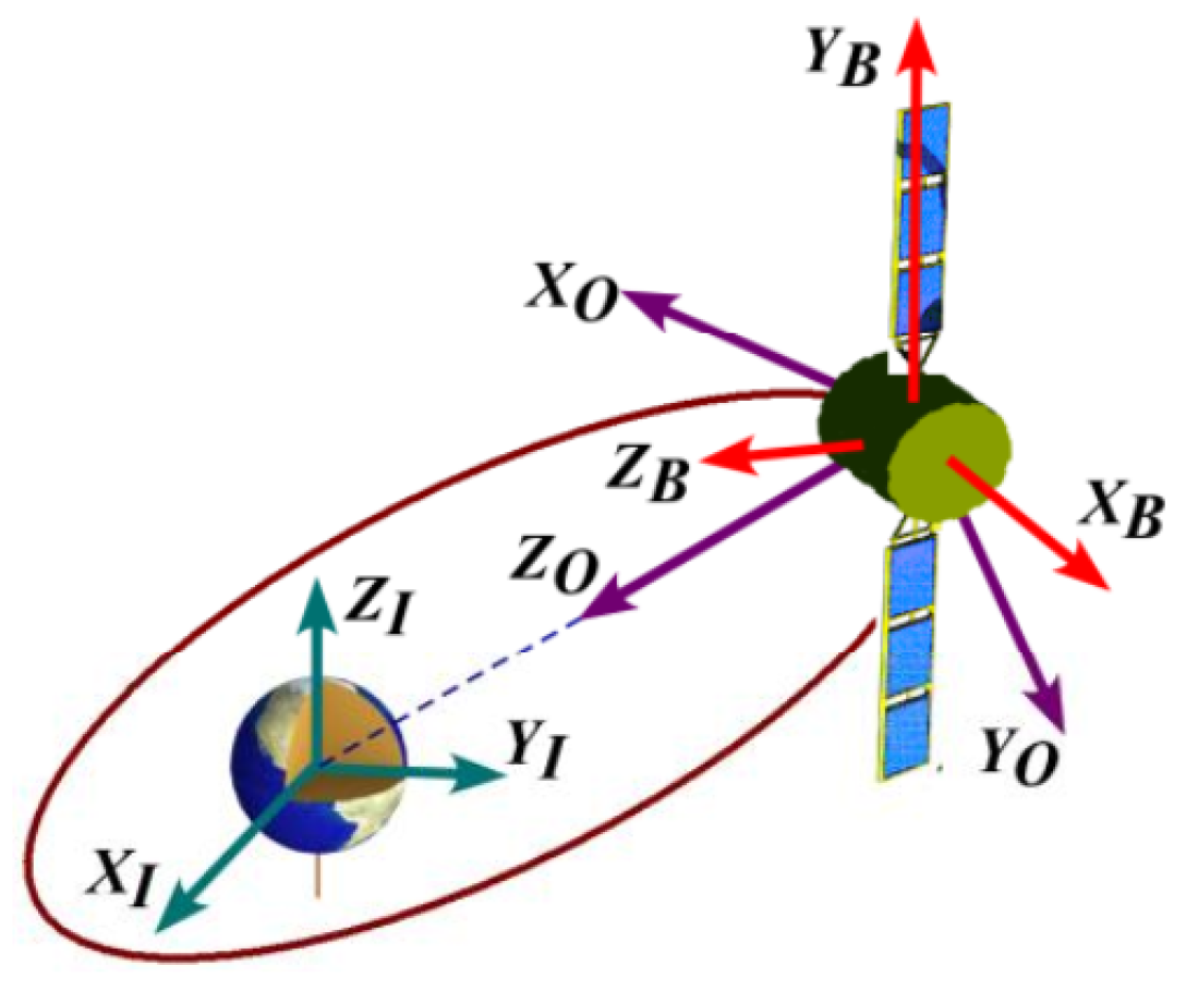
2.1. Equations of Motion of Rigid Spacecraft Attitude System

For representing the orientation of a rigid body in 3D space, three coordinate frames, depicted in Figure 1, are usually adopted. Here, the orbit reference, the inertial, and the body-fixed frames will be respectively represented by ${\mathcal{F}}_O$, ${\mathcal{F}}_I$, and ${\mathcal{F}}_B$. Let $\mathit{\sigma }\in {\mathbb{R}}^3$ be the modified Rodriguez parameters (MRPs) for the rigid spacecraft with respect to ${\mathcal{F}}_O$ and $\mathit{\omega }={[{\omega }_1,{\omega }_2,{\omega }_3]}^T$ refers to the inertial angular velocity with respect to ${\mathcal{F}}_I$ and described in ${\mathcal{F}}_B$. Therefore, the rigid spacecraft equations of motion can be described as [2]

$$\begin{array}{cc}\hfill \dot{\mathit{\sigma }}=& \mathit{G}\left(\mathit{\sigma }\right)\mathit{\omega }\hfill \\ \hfill \mathit{J}\dot{\mathit{\omega }}=& -{\mathit{\omega }}^{\times }\mathit{J}\mathit{\omega }+\mathbf{\tau }+\overline{\mathit{d}},\hfill \end{array}$$

(1)

where $\mathit{G}\left(\mathit{\sigma }\right)$ denotes the Jacobian matrix described as $\mathit{G}\left(\mathit{\sigma }\right)=\frac{1}{4}\left((1-{\mathit{\sigma }}^T\mathit{\sigma }){\mathit{I}}_3+2{\mathit{\sigma }}^{\times }+2\mathit{\sigma }{\mathit{\sigma }}^T\right)$, $\mathbf{\tau }\in {\mathbb{R}}^3$ is the control torque, $\overline{\mathit{d}}\in {\mathbb{R}}^3$ is environmental disturbance, and $\mathit{J}\in {\mathbb{R}}^{3\times 3}$ shows the inertia matrix described as $\mathit{J}={\mathit{J}}_0+\Delta \mathit{J}$, such that ${\mathit{J}}_0$ and $\Delta \mathit{J}$ are, respectively, the nominal and uncertain components of the inertia matrix.

Let us define ${\mathit{x}}_1=\mathit{\sigma }$ and ${\mathit{x}}_2=\dot{\mathit{\sigma }}$. Then, the system (1) could be described by

$$\begin{array}{cc}\hfill {\dot{\mathit{x}}}_1=& {\mathit{x}}_2,\hfill \\ \hfill {\dot{\mathit{x}}}_2=& \mathbf{\Gamma }+\mathit{u}+\mathit{d},\hfill \end{array}$$

(2)

where $\mathbf{\Gamma }={[{\Gamma }_1,{\Gamma }_2,{\Gamma }_3]}^T=\dot{\mathit{G}}\left({\mathit{x}}_{\mathbf{1}}\right)\mathit{\omega }-\mathit{G}\left({\mathit{x}}_1\right){\mathit{J}}_0^{-1}{\mathit{\omega }}^{\times }{\mathit{J}}_0\mathit{\omega }$, $\mathit{u}={[u_1,u_2,u_3]}^T=\mathit{G}\left({\mathit{x}}_1\right){\mathit{J}}_0^{-1}\mathit{\tau }$ and $\mathit{d}={[d_1,d_2,d_3]}^T=\mathit{G}\left({\mathit{x}}_1\right){\mathit{J}}_0^{-1}(\overline{\mathit{d}}-{\mathit{\omega }}^{\times }\Delta \mathit{J}\mathit{\omega }-\Delta \mathit{J}\dot{\mathit{\omega }})$.

Assumption 1. 

The uncertain component of the inertia matrix is bounded such that $\parallel \Delta \mathit{J}\parallel \le a_1$ where $a_1$ is an unknown positive scalar.

Assumption 2. 

The space disturbance is bounded such that $\parallel \overline{\mathit{d}}\parallel \le a_2$ where $a_2$ is an unknown positive scalar.

Remark 1. 

The system uncertainty is due to the payload movement, fuel consumption, and rotation of solar panels. On the other hand, the external disturbance stems from aerodynamic drag, gravity gradient moments, and solar radiation pressure. Based on Equation (2), when there exist the inertia matrix uncertainty $(\Delta \mathit{J})$ and the external disturbance $\left(\overline{\mathit{d}}\right)$, the attitude dynamics will be perturbed by $\mathit{d}$ which depends on the attitude $\left({\mathit{x}}_1\right)$, the angular velocity $\left(\mathit{\omega }\right)$, and the angular acceleration $\left(\dot{\mathit{\omega }}\right)$. The constants $a_1$ and $a_2$ show how these undesirable factors affect the system dynamics. Since the term $\mathit{d}$ is not used in the control design, the larger values of $a_1$ and $a_2$ mean that the knowledge about the system dynamics is not sufficient. The lack of adequate information about the system dynamics deteriorates the control performance or even system stability. Since the total uncertainty which is composed of the system uncertainty and disturbance enters in the input channel, it is a matched uncertainty and the sliding mode control can deal with that.

Remark 2. 

The main sources of perturbation in the rigid spacecraft attitude system are the inertia matrix uncertainty and the space disturbance torques. Since the total uncertainty does not vanish at the origin, it is considered as a nonvanishing perturbation. Thus, the origin is not the equilibrium point of the uncertain spacecraft attitude system. As a result, the problem of practically fixed-time stability of the perturbed attitude system is studied in this paper.

2.2. Preliminaries

Lemma 1. 

Consider a nonlinear system as [41]

$$\begin{array}{c}\hfill \dot{\mathit{x}}=\mathit{f}(t,\mathit{x},\mathit{d}).\end{array}$$

(3)

Let there exist a continuous positive-definite function $V\left(t\right)$ such that

$$\dot{V}\le -\frac{\pi }{\eta T_c}\left(V^{1-\frac{\eta }{2}}+V^{1+\frac{\eta }{2}}\right)$$

where $T_c>0$ represents the convergence time and $0<\eta <1$ is a real number. Then, the origin of the nonlinear system (3) is fixed-time stable with the convergence time $T_c$.

Lemma 2. 

For the given system (3) [42], if the following inequality holds

$$\dot{V}\le -\frac{\pi }{\eta T_c}\left(V^{1-\frac{\eta }{2}}+V^{1+\frac{\eta }{2}}\right)+\delta ,$$

then the system (3) is practically fixed-time stable with the convergence region described as

$$\left\{\underset{t\to T_c^{{}^{\prime }}}{lim}\mathit{x}|V\le min\left\{{\left(\frac{2\eta T_c\delta }{\pi }\right)}^{\frac{2}{2-\eta }},{\left(\frac{2\eta T_c\delta }{\pi }\right)}^{\frac{2}{2+\eta }}\right\}\right\}$$

where the parameter $T_c^{{}^{\prime }}$ represents the convergence time such that $T_c^{{}^{\prime }}<\sqrt{2}{T}_c$.

Lemma 3. 

For $z_1\in \mathbb{R}$, $z_2\in \mathbb{R}$ and positive constants ${\varsigma }_1>0$, ${\varsigma }_2>0$, ${\varsigma }_3>0$, one obtains [43]

$$\begin{array}{c}\hfill |z_1{|}^{{\varsigma }_1}|z_2{|}^{{\varsigma }_2}\le \frac{{\varsigma }_1}{{\varsigma }_1+{\varsigma }_2}{\varsigma }_3|z_1{|}^{{\varsigma }_1+{\varsigma }_2}+\frac{{\varsigma }_2}{{\varsigma }_1+{\varsigma }_2}{\varsigma }_3^{-\frac{{\varsigma }_1}{{\varsigma }_2}}{\left|z_2\right|}^{{\varsigma }_1+{\varsigma }_2}.\end{array}$$

(4)

Lemma 4. 

Consider a differential equation as [43]

$$\begin{array}{c}\hfill \dot{\widehat{z}}\left(t\right)={\varsigma }_1\varphi \left(t\right)-{\varsigma }_2\widehat{z}\left(t\right)-{\varsigma }_3{\widehat{z}}^{{\varsigma }_4}\left(t\right)\end{array}$$

(5)

in which ${\varsigma }_i>0$ for $i=1,2,3$ and ${\varsigma }_4>1$ are constants and $\varphi \left(t\right)$ is a non-negative function. If the initial condition satisfies $\widehat{z}\left(t_0\right)\ge 0$, then it is concluded that $\widehat{z}\left(t\right)\ge 0$ for $\forall t_0\ge 0$.

Lemma 5. 

For $z_2\ge z_1$ and ς>1, one obtains [43]

$$\begin{array}{c}\hfill z_1{(z_2-z_1)}^{\varsigma }\le \frac{\varsigma }{1+\varsigma }(z_2^{1+\varsigma }-z_1^{1+\varsigma }).\end{array}$$

(6)

Lemma 6. 

For any given $z_i\in {\mathbb{R}}^{+}(i=1,\dots ,n)$ and $\varsigma >0$, the following inequalities are satisfied [43]

$$\begin{array}{c}\hfill \left\{\begin{array}{cc}\sum _{i=1}^n{z}_i^{\varsigma }\ge {\left(\sum _{i=1}^n{z}_i\right)}^{\varsigma },\hfill & if0<\varsigma <1\hfill \\ \sum _{i=1}^n{z}_i^{\varsigma }\ge n^{1-\varsigma }{\left(\sum _{i=1}^n{z}_i\right)}^{\varsigma },\hfill & if\varsigma >1.\hfill \end{array}\right.\end{array}$$

(7)

Lemma 7. 

By virtue of ability of neural networks, a bounded, unknown nonlinear function $\mathbf{\Theta }\left(\mathit{X}\right)$ is approximated as a continuous function that is delimited on a compact set Ω. Then, there is a neural network ${{\mathit{W}}^{*}}^T\mathbf{\Phi }\left(\mathit{X}\right)$ such that [31]

$$\begin{array}{c}\hfill l\mathbf{\Theta }\left(\mathit{X}\right)={{\mathit{W}}^{*}}^T\mathbf{\Phi }\left(\mathit{X}\right)+\epsilon ,\end{array}$$

(8)

in which the input vector is denoted by $\mathit{X}\in \Omega$, the basis function of the neural network is represented by $\mathbf{\Phi }\left(\mathit{X}\right)\in {\mathbb{R}}^{\overline{v}}$ with $\overline{v}>1$ as the number of nodes, and the approximation error is denoted by ${\epsilon }_i$ which satisfies $|{\epsilon }_i|<{\epsilon }_N$ with ${\epsilon }_N$ as a positive constant. Moreover, ${\mathit{W}}^{*}$ shows the ideal weight matrix described as

$$\begin{array}{c}\hfill l{\mathit{W}}^{*}=arg\underset{\mathit{W}\in {\mathbb{R}}^{\overline{v}}}{min}\left\{\underset{\mathit{X}\in \Omega }{sup}|\mathbf{\Theta }\left(\mathit{X}\right)-{\mathit{W}}^T\mathbf{\Phi }\left(\mathit{X}\right)|\right\}\end{array}$$

(9)

in which $\mathit{W}\in {\mathbb{R}}^{\overline{v}}$ refers to the weight vector.

Definition 1. 

A positive, decreasing function $\rho \left(t\right)$ is named as a finite-time prescribed performance function (FTPPF) if it converges to ${\rho }_T$ within $T_f$ and stays thereafter. Here, $T_f$ is the convergence time of the FTPPF and ${\rho }_T$ shows its final value [44].

From an engineering point of view, this function gives the opportunity to the attitude control designer to determine any desired performance specifications for the spacecraft attitude in transient as well as steady state. We employ the following function as an FTPPF [38]

$$\rho \left(t\right)=\left\{\begin{array}{cc}\sqrt[c_1]{{\rho }_0^{c_1}-c_1{c}_{2}t}+{\rho }_T,\hfill & 0\le t<T_f,\hfill \\ {\rho }_T,\hfill & t\ge T_f.\hfill \end{array}\right.$$

(10)

where the positive constants ${\rho }_0$, $c_1$, and $c_2$ are rightly selected in accordance with the value of $T_f$, ${\rho }_T$, and $\rho \left(0\right)$. More specifically, ${\rho }_0=\rho \left(0\right)-{\rho }_T$, $c_2=\frac{{\rho }_0^{c_1}}{c_1{T}_f}$, and $0<c_1=\frac{b_1}{b_2}<1$ such that $b_1$ and $b_2$ are, respectively, positive odd and even integers.

2.3. Control Objective

The major control goal of this study is to propose a constrained control strategy for the rigid spacecraft attitude system expressed by Equation (2) such that:

• The closed-loop attitude system is practically fixed-time stable.
• The prescribed performance of the attitude MRPs $\sigma$ is satisfied. Unlike the existing constrained attitude controls for spacecraft [37,38,39,40], the proposed controller structure is quite simple.

Remark 3. 

The simplicity of the structure of the controller designed in this paper is due to the use of a time-varying gain in the sliding surface instead of using complicated constrained control approaches such as prescribed performance control [37,38,39,40]. In these works, to constrain the spacecraft attitude, a new variable is employed to convert the constrained attitude system into an equivalent unconstrained one. Then, the system dynamics will be rewritten based on the new transformed variable. It is proved that robust stabilization of this variable is equivalent to satisfying the constraint on the spacecraft attitude. However, the control inputs in [37,38,39,40] contain partial derivatives and intricate terms as a result of stabilizing the transformed error. This, in turn, makes the control design procedure and the controller structure quite complicated.

3. Nonsingular Constrained Switching Function Development

Motivated by [30], the following nonsingular constrained switching function (NCSF) $\mathit{S}\left(t\right)={[S_1\left(t\right),S_2\left(t\right),S_3\left(t\right)]}^T$$\in {\mathbb{R}}^3$ for the attitude system (2) is constructed

$$\begin{array}{c}\hfill \mathit{S}\left(t\right)={\mathit{x}}_1\left(t\right)+{\mathrm{Sig}}^{\frac{1}{1-{\eta }_1}}\left(\mathbf{{\rm Y}}({\mathit{x}}_2+(\mathbf{\alpha }+\mathbf{\gamma }){\mathit{x}}_1)\right),\end{array}$$

(11)

where $\frac{1}{2}<{\eta }_1<1$, $\mathbf{{\rm Y}}=\mathrm{diag}({{\rm Y}}_1,{{\rm Y}}_2,{{\rm Y}}_3)$ with ${{\rm Y}}_i=\frac{2{\eta }_1{T}_{c1}}{\pi \left(1+3^{\frac{{\eta }_1}{2}}{x}_{1i}^{2{\eta }_1}\right)}$, $T_{c1}>0$, $\mathbf{\alpha }=\mathrm{diag}({\alpha }_1,{\alpha }_2,{\alpha }_3)$ with ${\alpha }_i>0$, $\gamma =\mathrm{diag}({\gamma }_1,{\gamma }_2,{\gamma }_3)$ with ${\gamma }_i\left(t\right)={\int }_0^t{\lambda }_i\left(v\right)dv$, ${\lambda }_i\left(t\right)=tan\left(\frac{\pi {\kappa }_i\left(t\right)}{2}\right)$, ${\kappa }_i\left(t\right)=|\frac{{\mathit{\sigma }}_i\left(t\right)}{{\rho }_i\left(t\right)}{|}^{\vartheta }$, and $\vartheta >0$. Moreover, for the sake of simplicity, we define ${\mathrm{Sig}}^{\iota }\left(\mathit{x}\right)={\left[|x_1{|}^{\iota }\mathrm{sgn}\left(x_1\right),|x_2{|}^{\iota }\mathrm{sgn}\left(x_2\right),{\left|x_3\right|}^{\iota }\mathrm{sgn}\left(x_3\right)\right]}^T$ in which $\iota \in {\mathbb{R}}^{+}$ is a positive scalar and $\mathrm{sgn}(·)$ is the sign function.

Remark 4. 

In this paper, to provide fixed-time convergence of the system states, we have used the ${\mathit{Sig}}^{\iota }\left(x\right)$ function which is defined as ${\mathit{Sig}}^{\iota }\left(x\right)={\left|x\right|}^{\iota }\mathit{sgn}\left(x\right)$ where $sgn(·)$ denotes the standard sign function. It is worth mentioning that the function ${\mathit{Sig}}^{\iota }\left(x\right)$ used in the proposed control scheme is not a discontinuous function. In Figure 2, this function for $\iota =0.7$ has been compared with the functions x, $\mathit{sgn}\left(x\right)$, and $\left|x\right|$. As can be seen, the function ${\mathit{Sig}}^{\iota }\left(x\right)$ is continuously differentiable.

Once $S_i\left(t\right)=0$ is obtained, then one has

$$\begin{array}{c}\hfill {\dot{x}}_{1i}=-\frac{\pi }{2{\eta }_1{T}_{c1}}\left(3^{\frac{{\eta }_1}{2}}{x}_{1i}^{1+{\eta }_1}+x_{1i}^{1-{\eta }_1}\right)-({\alpha }_i+{\gamma }_i)x_{1i},\end{array}$$

(12)

which can be easily rewritten as

$$\begin{array}{c}\hfill x_{2i}+({\alpha }_i+{\gamma }_i)x_{1i}=-\frac{\pi }{2{\eta }_1{T}_{c1}}\left(3^{\frac{{\eta }_1}{2}}{x}_{1i}^{2{\eta }_1}+1\right)x_{1i}^{1-{\eta }_1}.\end{array}$$

(13)

Then, we have

$$\begin{array}{c}\hfill {{\rm Y}}_i(x_{2i}+({\alpha }_i+{\gamma }_i)x_{1i})=-x_{1i}^{1-{\eta }_1},\end{array}$$

(14)

where ${{\rm Y}}_i=\frac{2{\eta }_1{T}_{c1}}{\pi \left(3^{\frac{{\eta }_1}{2}}{x}_{1i}^{2{\eta }_1}+1\right)}$. If the absolute value of both sides of (14) is taken, it gives

$$\begin{array}{c}\hfill |{{\rm Y}}_i(x_{2i}+({\alpha }_i+{\gamma }_i)x_{1i}){|}^{\frac{1}{1-{\eta }_1}}=\left|x_{1i}\right|,\end{array}$$

(15)

Based on (14), one obtains

$$\begin{array}{c}\hfill \mathrm{sgn}\left({{\rm Y}}_i(x_{2i}+({\alpha }_i+{\gamma }_i)x_{1i})\right)=\mathrm{sgn}\left(-x_{1i}^{1-{\eta }_1}\right)=-\mathrm{sgn}\left(x_{1i}\right).\end{array}$$

(16)

Multiplying both sides of (15) and (16) yields

$$\begin{array}{c}\hfill {\mathrm{Sig}}^{\frac{1}{1-{\eta }_1}}\left({{\rm Y}}_i(x_{2i}+({\alpha }_i+{\gamma }_i)x_{1i})\right)=-x_{1i}\left(t\right).\end{array}$$

(17)

Then, the NFCTS (11) is constructed.

To prove the fixed-time convergence of the system states ${\mathit{x}}_1\left(t\right)$ and ${\mathit{x}}_2\left(t\right)$, let us construct a Lyapunov function candidate as $V_1={\mathit{x}}_1^T{\mathit{x}}_1$. Differentiating $V_1$ with respect to time along Equation (14) and using Lemma 6 will lead to

$$\begin{array}{cc}\hfill {\dot{V}}_1& =2\sum _{i=1}^3{x}_{1i}{\dot{x}}_{1i}=-\sum _{i=1}^3\frac{\pi }{{\eta }_1{T}_{c1}}\left(3^{\frac{{\eta }_1}{2}}{x}_{1i}^{2+{\eta }_1}+x_{1i}^{2-{\eta }_1}\right)-\sum _{i=1}^{3}2({\alpha }_i+{\gamma }_i)x_{1i}^2\hfill \\ \hfill & \le -\frac{\pi }{{\eta }_1{T}_{c1}}\left(V_1^{1+\frac{{\eta }_1}{2}}+V_1^{1-\frac{{\eta }_1}{2}}\right).\hfill \end{array}$$

(18)

Note that due to the definition of ${\gamma }_i={\int }_0^{t}tan\left(\frac{\pi }{2}|\frac{{\rho }_i\left(y\right)}{{\mathit{\sigma }}_i\left(y\right)}{|}^{\vartheta }\right)dy$, it is concluded that ${\gamma }_i$ is positive. Moreover, ${\alpha }_i>0$ is a design parameter. Thus, $-({\alpha }_i+{\gamma }_i)x_{1i}^2$ is always negative and can be dropped from inequality (18). By virtue of Lemma 1, it can be inferred that ${\mathit{x}}_1\left(t\right)$ and ${\mathit{x}}_2\left(t\right)$ will converge to the origin in a fixed time $T_{c1}$.

Taking the time-derivative of the NCSF (11) along with the system dynamics (2) gives

$$\begin{array}{cc}\hfill \dot{\mathit{S}}=& {\mathit{x}}_2+\frac{1}{1-{\eta }_1}\mathrm{diag}\left(|{{\rm Y}}_i(x_{2i}+({\alpha }_i+{\gamma }_i)x_{1i}){|}^{\frac{{\eta }_1}{1-{\eta }_1}}\right)(\dot{{\rm Y}}({\mathit{x}}_2+(\mathbf{\alpha }+\mathbf{\gamma }){\mathit{x}}_1)\hfill \\ \hfill & +{\rm Y}(\mathbf{\Gamma }+\mathit{u}+\mathit{d}+\lambda {\mathit{x}}_1+(\mathbf{\alpha }+\mathbf{\gamma }){\mathit{x}}_2))\hfill \\ \hfill =& \Lambda (\Psi +{\rm Y}\mathit{u}+{\mathit{\tau }}_d)-(\mathbf{\alpha }+\mathbf{\gamma })\mathit{S},\hfill \end{array}$$

(19)

where $\dot{{{\rm Y}}_i}=-\frac{\pi }{T_{c1}}{3}^{\frac{{\eta }_1}{2}}{{\rm Y}}_i^2{x}_{2i}{x}_{1i}^{2{\eta }_1-1}$, $\mathbf{\Lambda }=\mathrm{diag}({\Lambda }_1,{\Lambda }_2,{\Lambda }_3)$, ${\Lambda }_i=\frac{1}{1-{\eta }_1}{\left|{{\rm Y}}_i(x_{2i}+({\alpha }_i+{\gamma }_i)x_{1i})\right|}^{\frac{{\eta }_1}{1-{\eta }_1}}$, $\mathbf{\Psi }={\mathbf{{\rm Y}}}^{-1}\mathbf{\Omega }+\mathbf{{\rm Y}}(\mathbf{\Gamma }+\lambda {\mathit{x}}_1+(\mathbf{\alpha }+\mathbf{\gamma }){\mathit{x}}_2)+\dot{\mathbf{{\rm Y}}}({\mathit{x}}_2+(\mathbf{\alpha }+\mathbf{\gamma }){\mathit{x}}_1)$, $\mathbf{\Omega }=(1-{\eta }_1)\left({\mathrm{Sig}}^{\frac{1-2{\eta }_1}{1-{\eta }_1}}\left(\mathbf{{\rm Y}}({\mathit{x}}_2+(\mathbf{\alpha }+\mathbf{\gamma }){\mathit{x}}_1)\right)+(\mathbf{\alpha }+\mathbf{\gamma }){{\rm Y}}^2({\mathit{x}}_2+(\mathbf{\alpha }+\mathbf{\gamma }){\mathit{x}}_1)\right)$, and ${\mathit{\tau }}_d=\mathbf{{\rm Y}}\mathit{d}$.

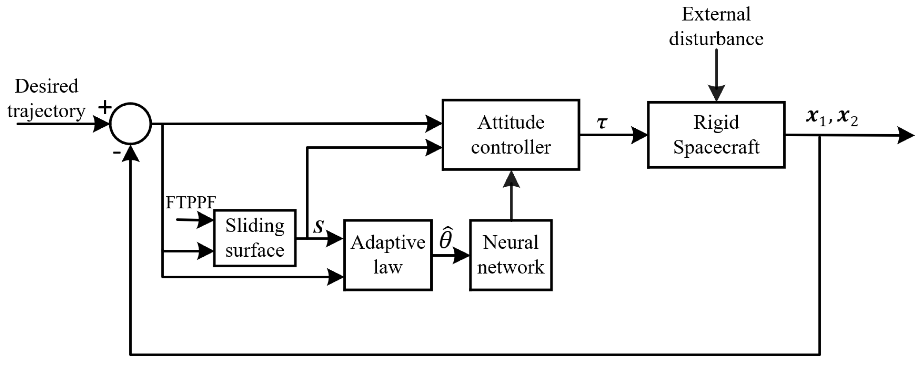
4. Adaptive Fixed-Time Attitude Control Development

Here, the principal goal is to derive an adaptive neural network-based attitude control scheme with fixed-time convergence for the attitude system described by Equation (2).

Due to the fact that the total uncertainty ${\mathit{\tau }}_d$ in (19) is not known in practice, neural networks can be utilized to approximate it. Motivated by [45], one has

$$\begin{array}{c}\hfill {\mathit{\tau }}_{di}+\frac{1}{2}{\Lambda }_i{S}_i={\mathit{W}}_i^T{\mathbf{\Phi }}_i\left({\mathit{X}}_n\right)+{\epsilon }_i,i=1,2,3\end{array}$$

(20)

where the weight vector is denoted by ${\mathit{W}}_i\in {\mathbb{R}}^{\overline{v}}$ with $\overline{v}>1$ as the number of nodes, the basis function of neural network is given by the following sigmoid form [46] ${\mathbf{\Phi }}_i\left({\mathit{X}}_n\right)=\frac{g_1}{g_2+exp(-{\mathit{x}}_n/g_3)}+g_4$ with $g_i$, $i=1,\dots ,4$ as constant parameters, the input vector is represented by ${\mathit{X}}_n={[{\mathit{x}}_1^T,{\mathit{x}}_2^T,{\mathit{\omega }}^T]}^T$ and the approximation error is denoted by ${\epsilon }_i$ which satisfies $|{\epsilon }_i|<{\epsilon }_N$ with ${\epsilon }_N$ as a positive constant.

According to the subsequent analysis, the following adaptive attitude control is proposed:

$$\begin{array}{cc}\hfill \mathit{u}=-{\mathbf{{\rm Y}}}^{-1}(& \mathbf{\Psi }+\frac{\pi }{{\eta }_2{T}_{c2}}\left({\left(\frac{1}{2}\right)}^{1-\frac{{\eta }_2}{2}}{\mathbf{\Lambda }}^{-1}{\mathit{\mu }}_{\nu }(\mathbf{\Lambda }){\mathit{S}}^{1-{\eta }_2}+3^{\frac{{\eta }_2}{2}}{2}^{{\eta }_2}{\left(\frac{1}{2}\right)}^{1+\frac{{\eta }_2}{2}}{\mathbf{\Lambda }}^{-1}{\mathit{\mu }}_{\nu }(\mathbf{\Lambda }){\mathit{S}}^{1+{\eta }_2}\right)\hfill \\ \hfill & +\frac{\widehat{\theta }}{2l^2}\mathbf{\Lambda }\mathrm{diag}\left({\mathbf{\Phi }}_i^T{\mathbf{\Phi }}_i\right)\mathit{S})\hfill \end{array}$$

(21)

where $\frac{1}{2}<{\eta }_2<1$, $T_{c2}>0$, $k_1>0$, $l>0$, and ${\mathit{\mu }}_{\nu }(\mathbf{\Lambda })=\mathrm{diag}({\mu }_{{\nu }_1}\left({\Lambda }_1\right),{\mu }_{{\nu }_2}\left({\Lambda }_2\right),{\mu }_{{\nu }_3}\left({\Lambda }_3\right))$ is defined as

$$\begin{array}{c}\hfill {\mu }_{{\nu }_i}\left({\Lambda }_i\right)=\left\{\begin{array}{cc}sin\left(\frac{\pi {\Lambda }_i}{2\nu }\right),\hfill & {\Lambda }_i\le \nu ,\hfill \\ 1,\hfill & \mathrm{otherwise},\hfill \end{array}\right.\end{array}$$

(22)

where $\nu >0$. Moreover, $\widehat{\theta }$ is the estimation of $\theta =max\{\parallel {\mathit{W}}_i{\parallel }^2\}$ for $i=1,2,3$ and it is updated by

$$\begin{array}{c}\hfill \dot{\widehat{\theta }}=\frac{k_1}{2l^2}\sum _{i=1}^3{\Lambda }_i^2{S}_i^2{\Phi }_i^T{\Phi }_i-k_2\widehat{\theta }-k_3{\widehat{\theta }}^{1+{\eta }_2},\end{array}$$

(23)

where $k_2={\left(\frac{\pi }{{\eta }_2{T}_{c2}}\right)}^{\frac{2}{2-{\eta }_2}}$ and $k_3=\frac{\pi (2+{\eta }_2)}{2{\eta }_2{T}_{c2}{k}_1^{\frac{{\eta }_2}{2}}(1+{\eta }_2)}$.

Theorem 1. 

Consider the attitude system given in (2). If the control law and the adaptive update law are designed as (21) and (23), respectively, then the system states ${\mathit{x}}_1$ and ${\mathit{x}}_2$ converge to the arbitrary small set containing the origin within a fixed time $T_c=T_{c1}+T_{c2}$.

Proof. 

Construct a Lyapunov function as $V_2=\frac{1}{2}{\mathit{S}}^T\mathit{S}+\frac{1}{2k_1}{\tilde{\theta }}^2$, where $\tilde{\theta }=\theta -\widehat{\theta }$. The derivative of $V_2$ with respect to time along Equation (19) and using (20) yields

$$\begin{array}{cc}\hfill {\dot{V}}_2=& {\mathit{S}}^T\mathbf{\Lambda }\left(\mathbf{\Psi }+\mathbf{{\rm Y}}\mathit{u}+{\mathit{\tau }}_d\right)-{\mathit{S}}^T(\mathbf{\alpha }+\mathbf{\gamma })\mathit{S}-\frac{1}{k_1}\tilde{\theta }\dot{\widehat{\theta }}\hfill \\ \hfill =& {\mathit{S}}^T\mathbf{\Lambda }\left(\mathbf{\Psi }+\mathbf{{\rm Y}}\mathit{u}-\frac{1}{2}\mathbf{\Lambda }\mathit{S}+{\mathit{W}}^T\mathbf{\Phi }\left({\mathit{X}}_n\right)+\epsilon \right)-{\mathit{S}}^T(\mathbf{\alpha }+\mathbf{\gamma })\mathit{S}-\frac{1}{k_1}\tilde{\theta }\dot{\widehat{\theta }}\hfill \end{array}$$

(24)

Utilizing the well-known Young’s inequality [47] and using the fact $\theta =max\{\parallel {\mathit{W}}_i{\parallel }^2\}$, the following inequality holds

$$\begin{array}{cc}\hfill l{\mathit{S}}^T\mathbf{\Lambda }({\mathit{W}}^T\mathbf{\Phi }\left({\mathit{X}}_n\right)+\epsilon )& l\le \frac{1}{2l^2}\sum _{i=1}^3{S}_i^2{W}_i^2{\Lambda }_i^2{\Phi }_i^T{\Phi }_i+\frac{3l^2}{2}+\frac{1}{2}{\parallel {\mathit{S}}^T\mathbf{\Lambda }\parallel }^2+\frac{3{\epsilon }_N^2}{2}\hfill \\ \hfill & l\le \frac{\theta }{2l^2}\sum _{i=1}^3{S}_i^2{\Lambda }_i^2{\Phi }_i^T{\Phi }_i+\frac{3l^2}{2}+\frac{1}{2}{\parallel {\mathit{S}}^T\mathbf{\Lambda }\parallel }^2+\frac{3{\epsilon }_N^2}{2}\hfill \end{array}$$

(25)

When $\parallel \mathbf{\Lambda }\parallel >\nu$, the function ${\mu }_{{\nu }_i}\left({\Lambda }_i\right)$ is equal to 1. Then, substituting the control law (21) and the update law (23) into (24) and using (25), one has

$$\begin{array}{cc}\hfill {\dot{V}}_2\le & -\frac{\pi }{{\eta }_2{T}_{c2}}\left({\left(\frac{1}{2}\right)}^{1-\frac{{\eta }_2}{2}}{\mathit{S}}^{2-{\eta }_2}+3^{\frac{{\eta }_2}{2}}{2}^{{\eta }_2}{\left(\frac{1}{2}\right)}^{1+\frac{{\eta }_2}{2}}{\mathit{S}}^{2+{\eta }_2}\right)-\frac{\widehat{\theta }}{2l^2}\sum _{i=1}^3{S}_i^2{\Lambda }_i^2{\Phi }_i^T{\Phi }_i\hfill \\ \hfill & +\frac{\theta }{2l^2}\sum _{i=1}^3{S}_i^2{\Lambda }_i^2{\Phi }_i^T{\Phi }_i+\frac{3l^2}{2}+\frac{3{\epsilon }_N^2}{2}-\frac{\tilde{\theta }}{2l^2}\sum _{i=1}^3{S}_i^2{\Lambda }_i^2{\Phi }_i^T{\Phi }_i+\frac{k_2}{k_1}\tilde{\theta }\widehat{\theta }+\frac{k_3}{k_1}\tilde{\theta }{\widehat{\theta }}^{1+{\eta }_2}\hfill \\ \hfill \le & -\frac{\pi }{{\eta }_2{T}_{c2}}\left({\left(\frac{1}{2}{\parallel \mathit{S}\parallel }^2\right)}^{1-\frac{{\eta }_2}{2}}+2^{{\eta }_2}{\left(\frac{1}{2}{\parallel \mathit{S}\parallel }^2\right)}^{1+\frac{{\eta }_2}{2}}\right)+\frac{k_2}{k_1}\tilde{\theta }\widehat{\theta }+\frac{k_3}{k_1}\tilde{\theta }{\widehat{\theta }}^{1+{\eta }_2}+{\delta }_1\hfill \end{array}$$

(26)

where ${\delta }_1=\frac{3l^2}{2}+\frac{3{\epsilon }_N^2}{2}$. Note that since $\tilde{\theta }=\theta -\widehat{\theta }$, the three terms $-\frac{\widehat{\theta }}{2l^2}{\sum }_{i=1}^3{S}_i^2{\Lambda }_i^2{\Phi }_i^T{\Phi }_i$, $\frac{\theta }{2l^2}{\sum }_{i=1}^3{S}_i^2{\Lambda }_i^2{\Phi }_i^T{\Phi }_i$, and $-\frac{\tilde{\theta }}{2l^2}{\sum }_{i=1}^3{S}_i^2{\Lambda }_i^2{\Phi }_i^T{\Phi }_i$ are simplified and removed from the right-hand side of the inequality (26). Based on the Young’s inequality, one obtains

$$\begin{array}{c}\hfill \frac{k_2}{k_1}\tilde{\theta }\widehat{\theta }=\frac{k_2}{k_1}\tilde{\theta }(\theta -\tilde{\theta })\le -\frac{k_2}{2k_1}{\tilde{\theta }}^2+\frac{k_2}{2k_1}{\theta }^2.\end{array}$$

(27)

Substituting (27) into (26) gives

$$\begin{array}{cc}\hfill {\dot{V}}_2\le & -\frac{\pi }{{\eta }_2{T}_{c2}}\left({\left(\frac{1}{2}{\parallel \mathit{S}\parallel }^2\right)}^{1-\frac{{\eta }_2}{2}}+2^{{\eta }_2}{\left(\frac{1}{2}{\parallel \mathit{S}\parallel }^2\right)}^{1+\frac{{\eta }_2}{2}}\right)\hfill \\ & -\frac{k_2}{2k_1}{\tilde{\theta }}^2+\frac{k_2}{2k_1}{\theta }^2+\frac{k_3}{k_1}\tilde{\theta }{\widehat{\theta }}^{1+{\eta }_2}+{\delta }_1.\hfill \end{array}$$

(28)

By virtue of Lemma 3 and defining $z_1=1$, $z_2=\frac{k_2}{2k_1}{\tilde{\theta }}^2$, ${\varsigma }_1=\frac{{\eta }_2}{2}$, ${\varsigma }_2=1-\frac{{\eta }_2}{2}$ and ${\varsigma }_3={\left(\frac{2-{\eta }_2}{2}\right)}^{\frac{2-{\eta }_2}{{\eta }_2}}$, one obtains

$$\begin{array}{c}\hfill {\left(\frac{k_2}{2k_1}{\tilde{\theta }}^2\right)}^{1-\frac{{\eta }_2}{2}}\le \frac{{\eta }_2}{2}{\left(\frac{2-{\eta }_2}{2}\right)}^{\frac{2-{\eta }_2}{{\eta }_2}}+\frac{k_2}{2k_1}{\tilde{\theta }}^2.\end{array}$$

(29)

According to the update law (23) and using Lemma 4, it can be concluded that $\widehat{\theta }\ge 0$, and then, $\theta \ge \tilde{\theta }$. Therefore, by virtue of Lemma 5 and defining $z_1=\tilde{\theta }$ and $z_2=\theta$, we have

$$\begin{array}{c}\hfill \tilde{\theta }{\widehat{\theta }}^{1+{\eta }_2}=\tilde{\theta }{(\theta -\tilde{\theta })}^{1+{\eta }_2}\le \frac{1+{\eta }_2}{2+{\eta }_2}({\theta }^{2+{\eta }_2}-{\tilde{\theta }}^{2+{\eta }_2}).\end{array}$$

(30)

Now, substituting (29) and (30) into (28) results in

$$\begin{array}{cc}\hfill {\dot{V}}_2\le & -\frac{\pi }{{\eta }_2{T}_{c2}}{\left(\frac{1}{2}{\parallel \mathbf{S}\parallel }^2\right)}^{1-\frac{{\eta }_2}{2}}-{\left(\frac{k_2}{2k_1}{\tilde{\theta }}^2\right)}^{1-\frac{{\eta }_2}{2}}-\frac{\pi }{{\eta }_2{T}_{c2}}{2}^{{\eta }_2}{\left(\frac{1}{2}{\parallel \mathbf{S}\parallel }^2\right)}^{1+\frac{{\eta }_2}{2}}\hfill \\ \hfill & -\frac{2^{1+\frac{{\eta }_2}{2}}{k}_3{k}_1^{\frac{{\eta }_2}{2}}(1+{\eta }_2)}{2+{\eta }_2}{\left(\frac{1}{2k_1}{\tilde{\theta }}^2\right)}^{1+\frac{{\eta }_2}{2}}+{\delta }_2\hfill \\ \hfill \le & -\frac{\pi }{{\eta }_2{T}_{c2}}\left(V_2^{1-\frac{{\eta }_2}{2}}+V_2^{1+\frac{{\eta }_2}{2}}\right)+{\delta }_2\hfill \end{array}$$

(31)

where ${\delta }_2=\frac{{\eta }_2}{2}{\left(\frac{2-{\eta }_2}{2}\right)}^{\frac{2-{\eta }_2}{{\eta }_2}}+\frac{k_2}{2k_1}{\theta }^2+\frac{k_3(1+{\eta }_2){\theta }^{2+{\eta }_2}}{k_1(2+{\eta }_2)}+{\delta }_1$.

Thus, by virtue of Lemma 2, the system states ${\mathit{x}}_1$ and ${\mathit{x}}_2$ are driven to the following arbitrary small region $\Delta$ or enter the region ${\mathcal{R}}_2$ during the fixed time $T_{c2}$.

$$\Delta =\left\{\underset{t\to T_{c2}}{lim}\mathbf{S}|V_2\le min{\left\{{\left(\frac{2{\eta }_2{T}_{c2}{\delta }_2}{\pi }\right)}^{\frac{2}{2-{\eta }_2}},(\frac{2{\eta }_2{T}_{c2}{\delta }_2}{\pi }\right)}^{\frac{2}{2+{\eta }_2}}\right\}\}.$$

In ${\mathcal{R}}_2$, defining $\mathbf{\chi }={\mathit{x}}_2+(\mathbf{\alpha }+\mathbf{\gamma }){\mathit{x}}_1$, the objective is to prove that the $\mathbf{\chi }=\mathbf{0}$ (which is the reason of singularity) is not attractive except for the origin $({\mathit{x}}_1,{\mathit{x}}_2)=\mathbf{0}$. To this end, at a close vicinity of $\mathbf{\chi }=\mathbf{0}$, then $\mathbf{\Lambda }=\mathbf{\Omega }=\mathbf{\Psi }=\mathbf{0}$ and $\mathit{S}={\mathit{x}}_1$ will be obtained. Based on the definition of ${\mu }_v(\Lambda )$ in (22), when ${\Lambda }_i\to 0$, then ${\Lambda }_i^{-1}{\mu }_{{\nu }_i}\left({\Lambda }_i\right)\to 1.$ Substituting $\mathbf{\Lambda }=\mathbf{\Omega }=\mathbf{\Psi }=\mathbf{0}$ and $\mathit{S}={\mathit{x}}_1$ into the control input, one has

$$\begin{array}{c}\hfill l\mathit{u}=-{\mathbf{{\rm Y}}}^{-1}\frac{\pi }{{\eta }_2{T}_{c2}}\left({\left(\frac{1}{2}\right)}^{1-\frac{{\eta }_2}{2}}{\mathit{x}}_1^{1-{\eta }_2}+3^{\frac{{\eta }_2}{2}}{\left(\frac{1}{2}\right)}^{1+\frac{{\eta }_2}{2}}{2}^{{\eta }_2}{\mathit{x}}_1^{1+{\eta }_2}\right)-\mathbf{\Gamma }.\end{array}$$

(32)

In order to show that the state trajectories will not settle down in $\mathbf{\chi }=0$, the derivative of $\mathbf{\chi }$ with respect to time and along the system (2) is taken, and substituting the approximated control input (32) is then given as

$$\begin{array}{c}\hfill l\dot{\mathbf{\chi }}=-{\mathbf{{\rm Y}}}^{-1}\frac{\pi }{{\eta }_2{T}_{c2}}\left({\left(\frac{1}{2}\right)}^{1-\frac{{\eta }_2}{2}}{\mathit{x}}_1^{1-{\eta }_2}+{\left(\frac{1}{2}\right)}^{1+3^{\frac{{\eta }_2}{2}}\frac{{\eta }_2}{2}}{2}^{{\eta }_2}{\mathit{x}}_1^{1+{\eta }_2}\right)+(\mathbf{\lambda }+{(\mathbf{\alpha }+\mathbf{\gamma })}^2){\mathit{x}}_1+\mathit{d}.\end{array}$$

(33)

The main objective is to show that $\mathbf{\chi }=0$ will be reached only if the state trajectories reach the origin, i.e., $({\mathit{x}}_1,{\mathit{x}}_2)=\mathbf{0}$. To be more exact, if $\dot{\mathbf{\chi }}=0$ is achieved, it means that the trajectories converge to $\mathbf{\chi }=0$ and stay thereafter. Thus, if for a non-zero value of ${\mathit{x}}_1$, then $\dot{\mathbf{\chi }}=0$ is reached, it conveys that the origin is not the only stable equilibrium point and there is another point in the state space where the state trajectories converge to.

Even if the uncertainty term $\mathit{d}$ is ignored, when ${\mathit{x}}_1\ne 0$, then $\dot{\mathbf{\chi }}\ne 0$ which means that $\mathbf{\chi }=0$ is not attractive except for the origin and the system states transgress ${\mathcal{R}}_2$ into ${\mathcal{R}}_1$. Therefore, it can be inferred that system trajectories converge to the residual set $\Delta$ from anywhere in the state space and the closed-loop system is practically fixed-time stable. Once the NCSF (11) converges to the set $|S_i|\le \Delta$, then one obtains

$$\begin{array}{c}\hfill S_i\left(t\right)=x_{1i}\left(t\right)+{\mathrm{Sig}}^{\frac{1}{1-{\eta }_1}}\left({{\rm Y}}_i(x_{2i}+({\alpha }_i+{\gamma }_i)x_{1i})\right)={\xi }_i,\left|{\xi }_i\right|<\Delta .\end{array}$$

(34)

Following Equations (12)–(17) for $S_i={\xi }_i$, Equation (34) is simplified as

$$\begin{array}{c}\hfill {\dot{x}}_{1i}+\frac{\pi }{2{\eta }_1{T}_{c1}}\left(3^{\frac{{\eta }_1}{2}}{x}_{1i}^{1+{\eta }_1}+x_{1i}^{1-{\eta }_1}\right)+\left(\alpha +{\gamma }_i-\frac{{\xi }_i}{x_{1i}}\right)x_{1i}=0.\end{array}$$

(35)

As long as $\alpha$ is selected to satisfy $\alpha +{\gamma }_i-\frac{{\xi }_i}{x_{1i}}>0$, Equation (35) is equivalent to Equation (14). Therefore, the spacecraft attitude is practically fixed-time stable and the convergence region is given as $|x_{1i}|<\frac{|{\xi }_i|}{{\alpha }_i}<\frac{\Delta }{{\alpha }_i}$. □

Remark 5. 

In the existing fixed-time sliding mode-based controls in [24,25,26,27,28,29,30,31], the convergence time is a function of twelve parameters; six parameters for the sliding surface and six parameters for the control input. Hence, to achieve a prescribed settling time for the closed-loop system, a complicated parameter tuning is needed. Since these parameters contribute to determining the transient and steady-state characteristics, it is difficult to obtain the desired convergence time without deteriorating the performance in transient and steady state. However, the proposed control framework in this paper guarantees that the system states converge to zero before $T_c=T_{c1}+T_{c2}$ in which $T_{c1}$ and $T_{c2}$ explicitly appear in the NCSF (11) and the control law (21), respectively. Moreover, the proposed control scheme is able to satisfy the desired performance in transient and steady state through tuning the parameters of the performance function. Therefore, the prespecified convergence time as well as the performance characteristics in time domain can be obtained. For instance, if the parameter ${\rho }_T$ in the performance function (10) decreases, the ultimate value of attitude is reduced and, consequently, the pointing accuracy is improved.

Remark 6. 

Because of the use of the non-integer power, which is less than one, to provide fixed-time stability, a negative power appears in the dynamics of the sliding surface and results in the singularity issue. To resolve this problem, one way would be to use a piecewise continuous switching function [26,29,48,49]. However, due to the fact $\frac{1}{2}<{\eta }_1<1$, it is concluded that $\frac{{\eta }_1}{1-{\eta }_1}>0$ holds and the time derivative of the suggested NCSF in (19) contains no negative power and, consequently, no singularity happens. Thus, in contrast to the aforementioned studies, the singularity is avoided without having to use any piecewise continuous switching function.

Remark 7. 

The suggested attitude control input (21) is composed of the term ${\lambda }_i{x}_{1i}$ in ${{\rm Y}}_i$. According to the definition of ${\lambda }_i\left(t\right)=tan\left(\frac{\pi {\kappa }_i\left(t\right)}{2}\right)$ and ${\kappa }_i\left(t\right)=|\frac{x_{1i}\left(t\right)}{{\rho }_i\left(t\right)}{|}^{\vartheta }$, it is inferred that if the attitude trajectory $x_{1i}$ tends to the boundary of the FTPPF ${\rho }_i$, the non-dynamic adaptive gain ${\lambda }_i$ increases and, as a result, the control effort rises to prevent the attitude from contacting the performance function and violating the constraint. Hence, the approach utilized here is able to successfully meet the constraint on the attitude trajectory such that there is no need to apply the existing complicated constrained controls.

Remark 8. 

The diagram of the new NN-based control which is composed of the spacecraft, the neural network, and the attitude controller is illustrated in Figure 3.

Remark 9. 

The control parameters are selected by trial and error until the desired control performance is acquired. However, the following points are considered to obtain a better understanding on the effect of each parameter on the control performance and to tune them appropriately.

• The fractional powers ${\eta }_1$ and ${\eta }_2$ have significant effect on the convergence behavior. If they are selected too small, the faster and more accurate convergence will be obtained; however, the control input increases.
• The parameters $T_{c1}$ and $T_{c2}$ represent the settling time. Hence, smaller $T_{c1}$ and $T_{c2}$ result in a faster convergence. Nonetheless, the needed control input will go up.
• The parameter α contributes to the convergence rate and control input. Indeed, if it is selected large enough, the system states are quickly stabilized at a price of large control input.
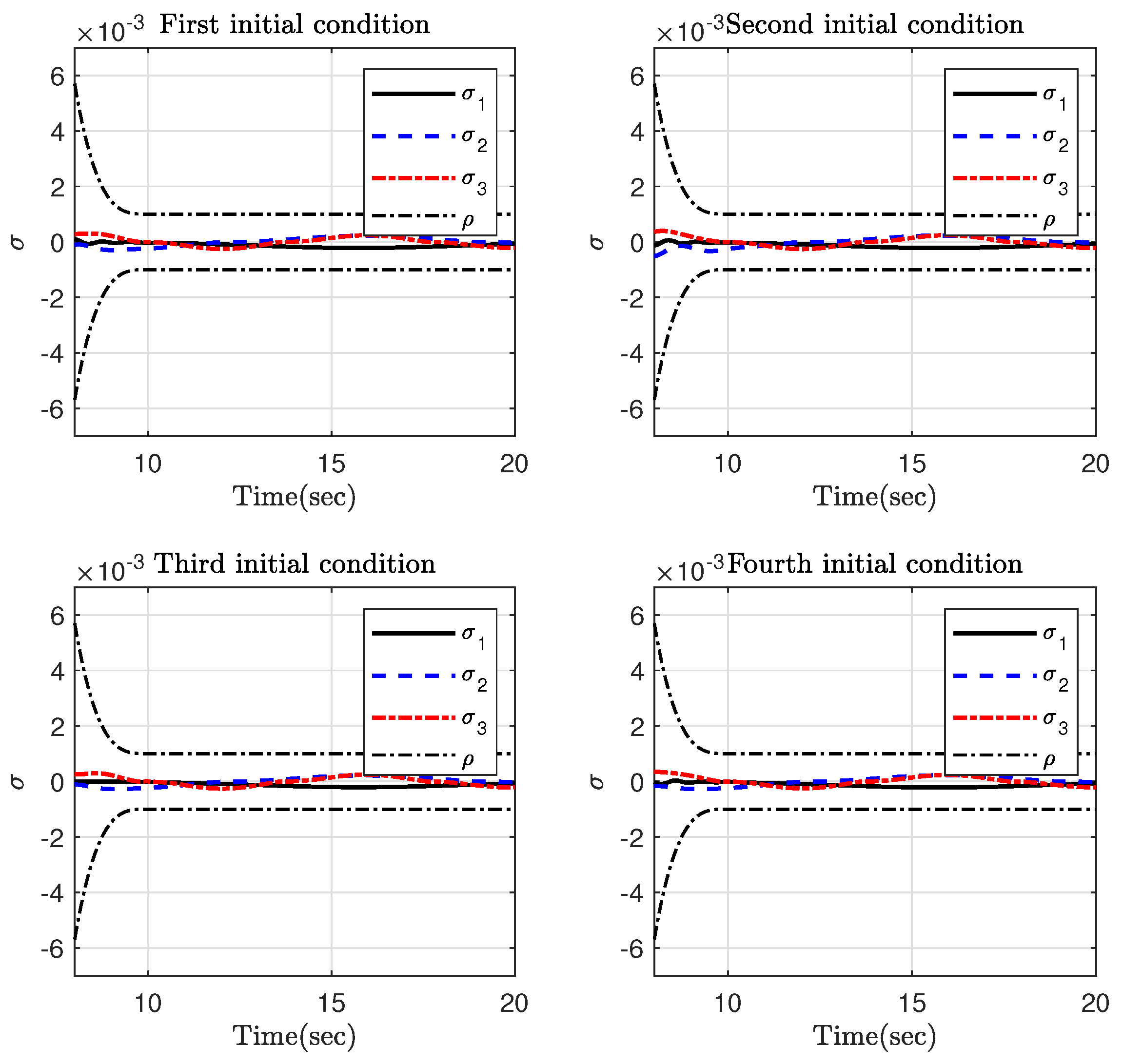
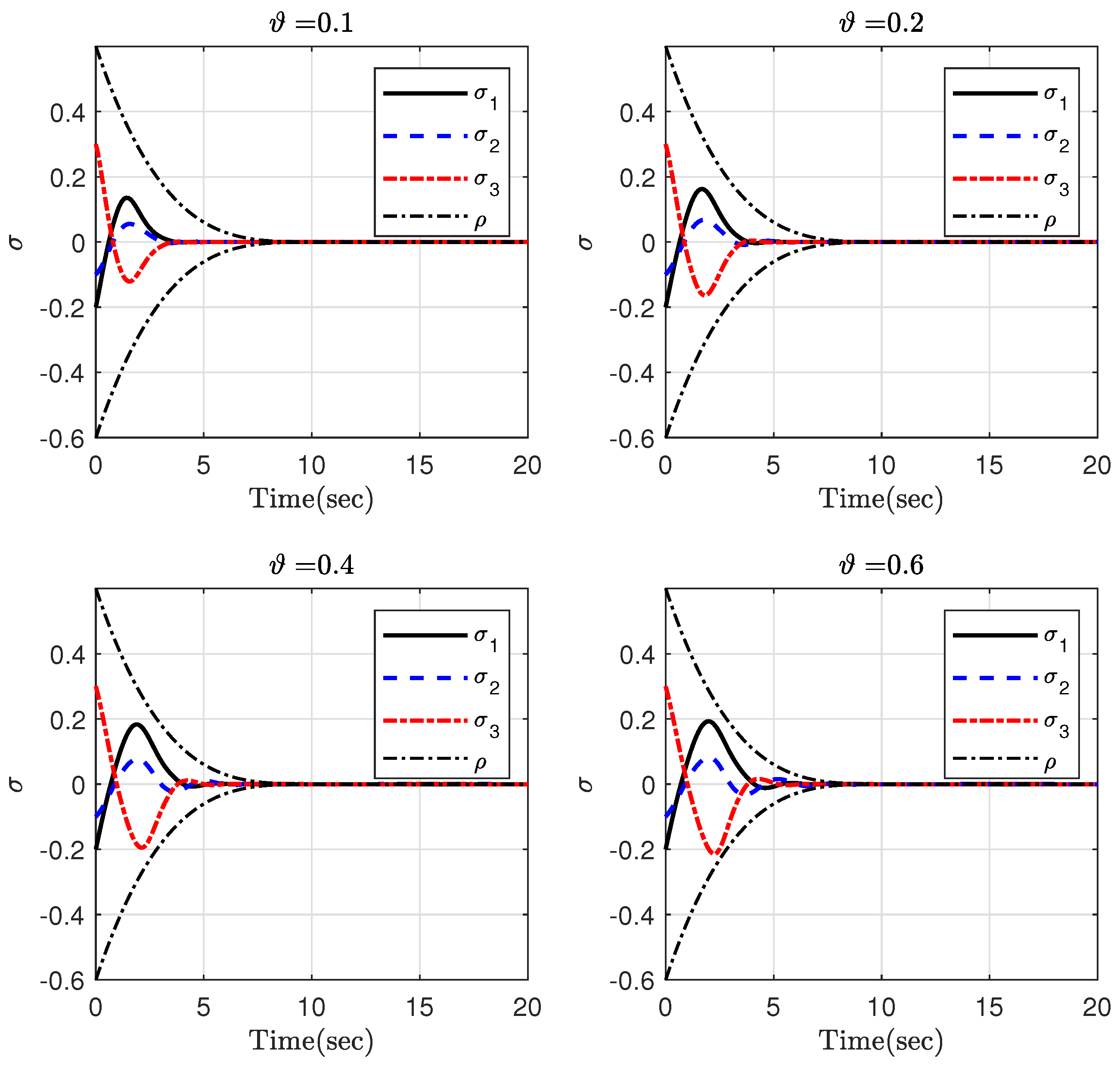
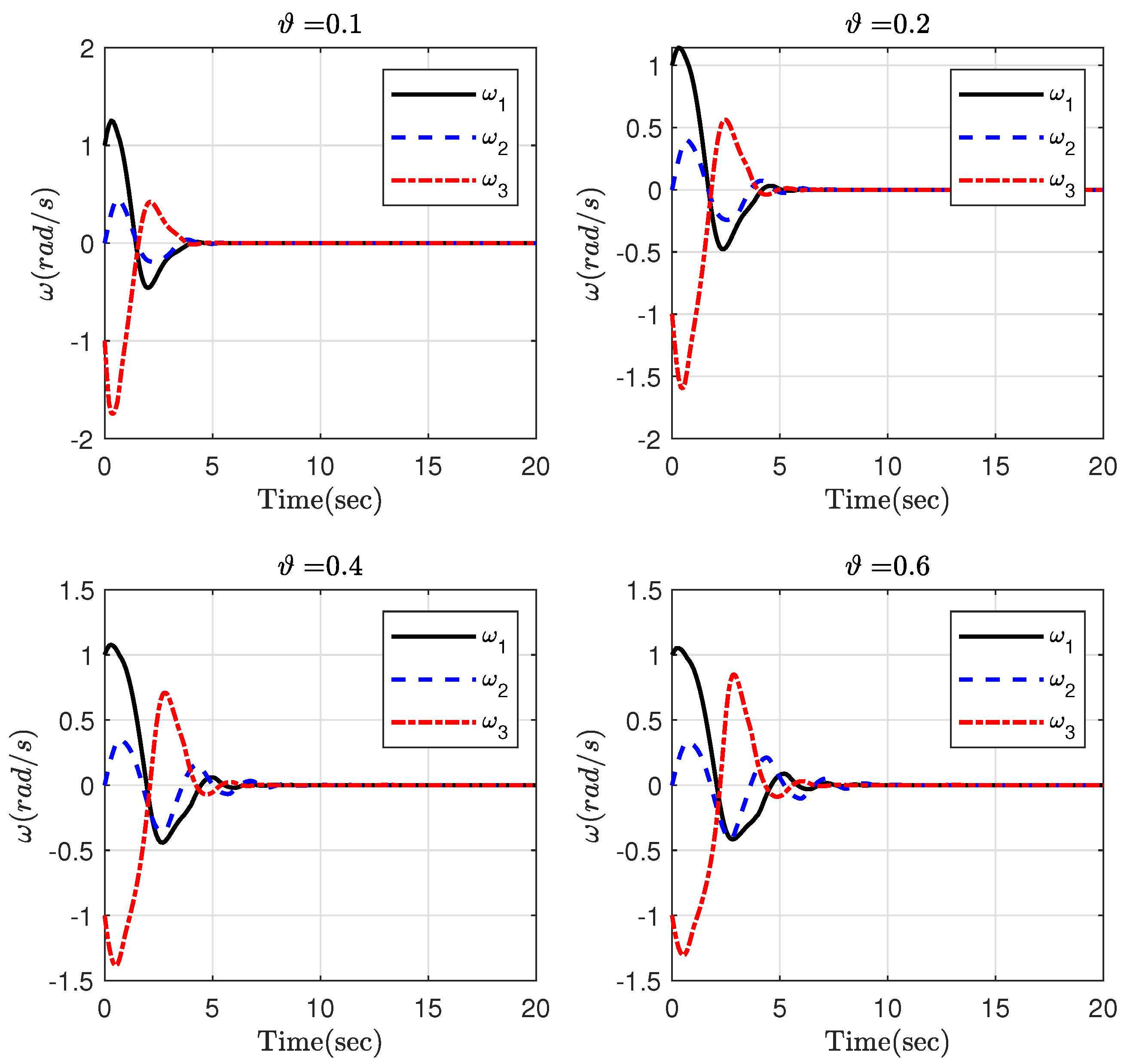
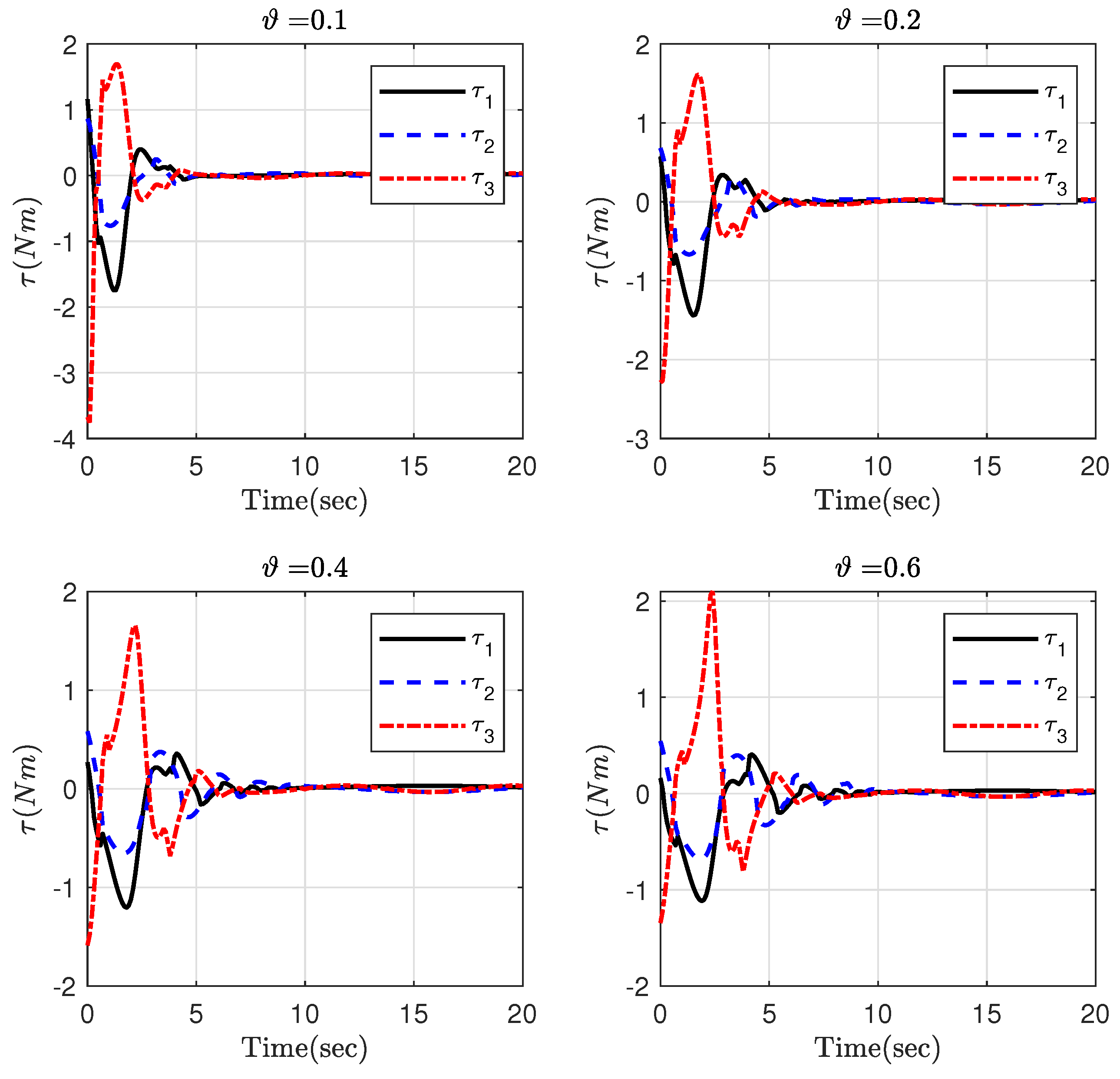
• Since $0<\kappa <1$, then a larger value of ϑ means that the attitude trajectory is allowed to approach the performance function boundary.
• The parameters of the performance function are selected based on the maximum permitted overshoot, the convergence time, and the ultimate attitude value.

Remark 10. 

Disturbance observer, as an active disturbance rejection control approach, has been widely employed to cope with the total disturbance owing to the system uncertainty and external disturbance [50,51,52]. In this case, the total disturbance is estimated by the observer and the estimated signal is used as a feedforward signal in the controller. Therefore, the control performance is improved. However, since the spacecraft attitude system is nonlinear, the separation principle is not satisfied and the stability analysis must be proved considering both the observer and the controller. Moreover, a disturbance observer-based control has a more complicated control structure. On the other hand, neural network-based adaptive control can be a suitable alternative which provides desired performance and does not have complexity of the disturbance observers.

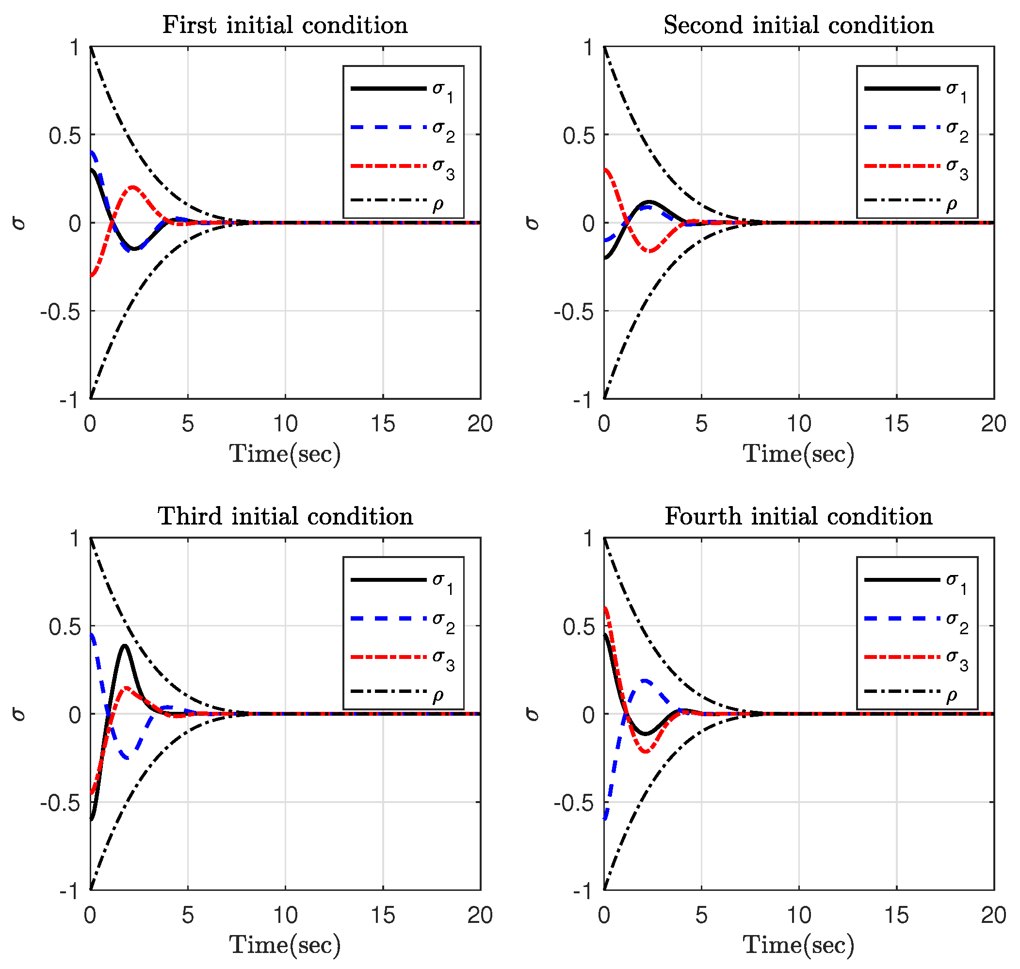
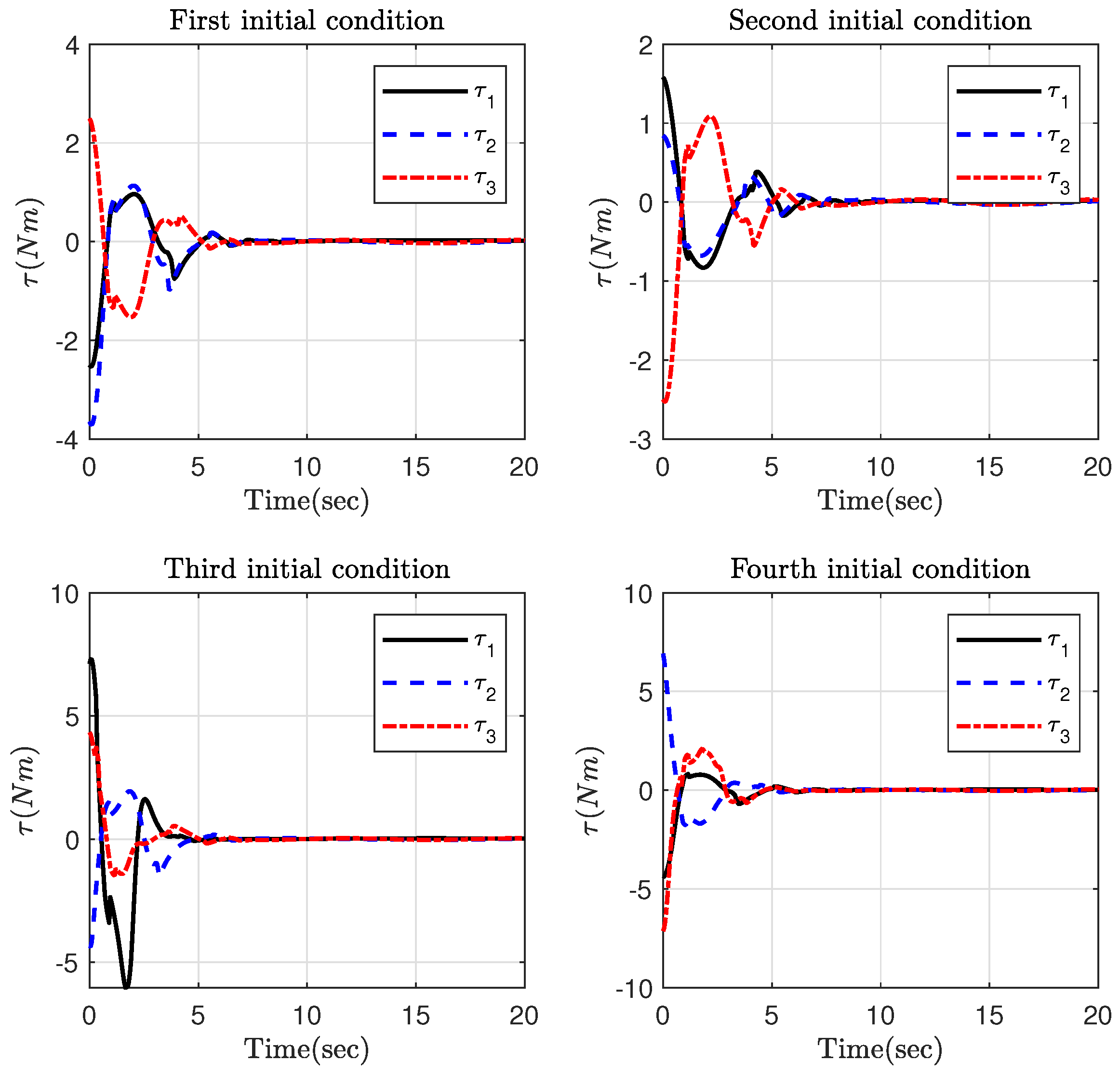
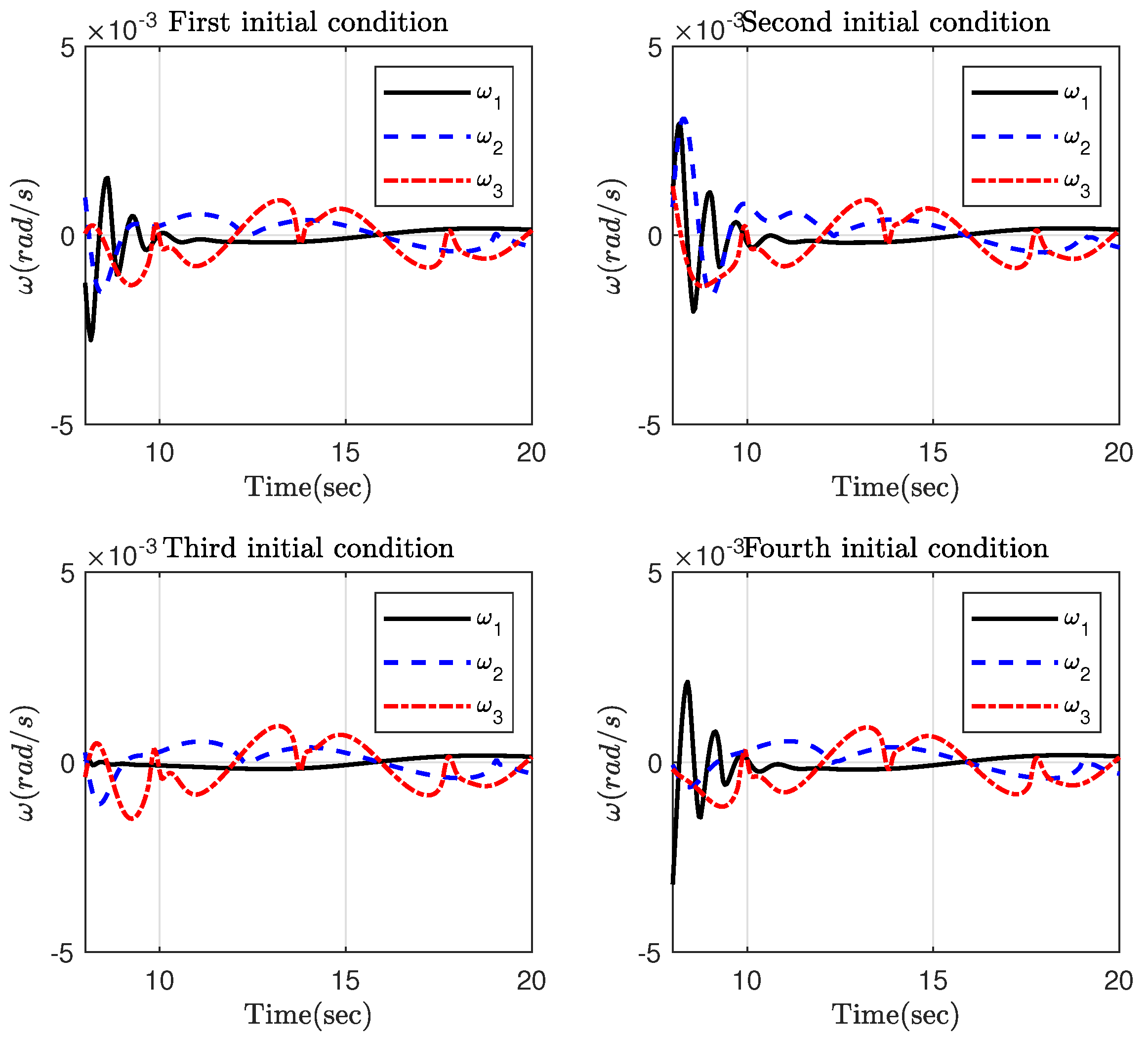
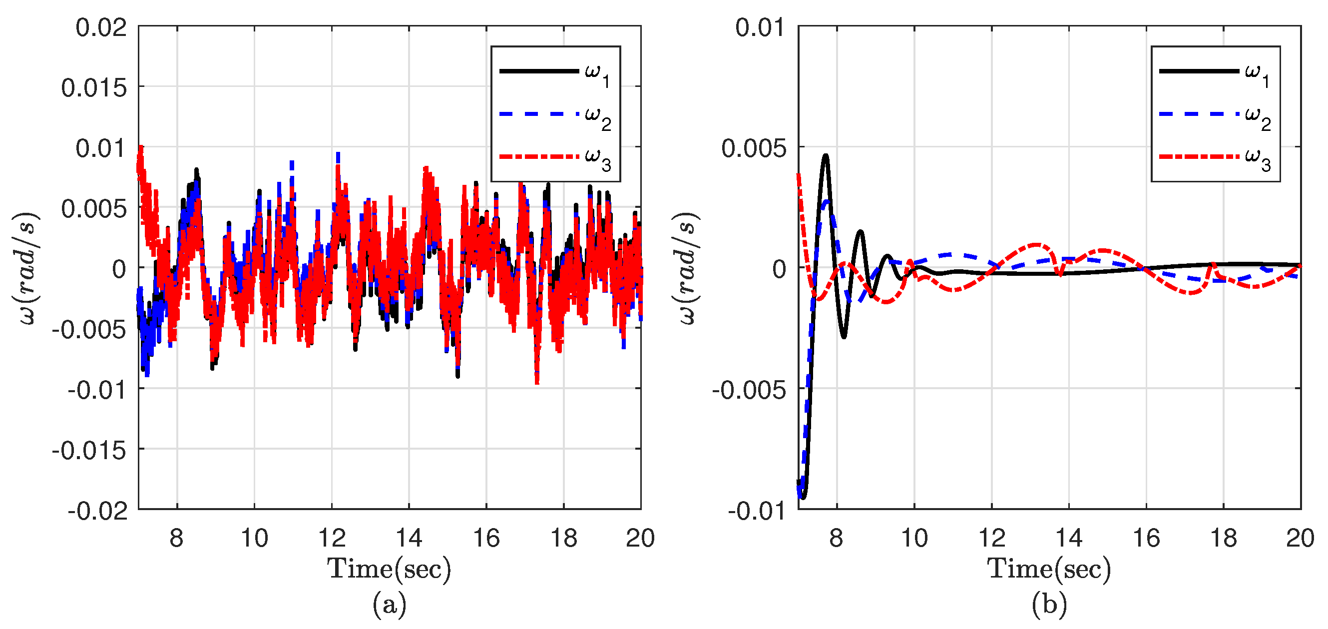
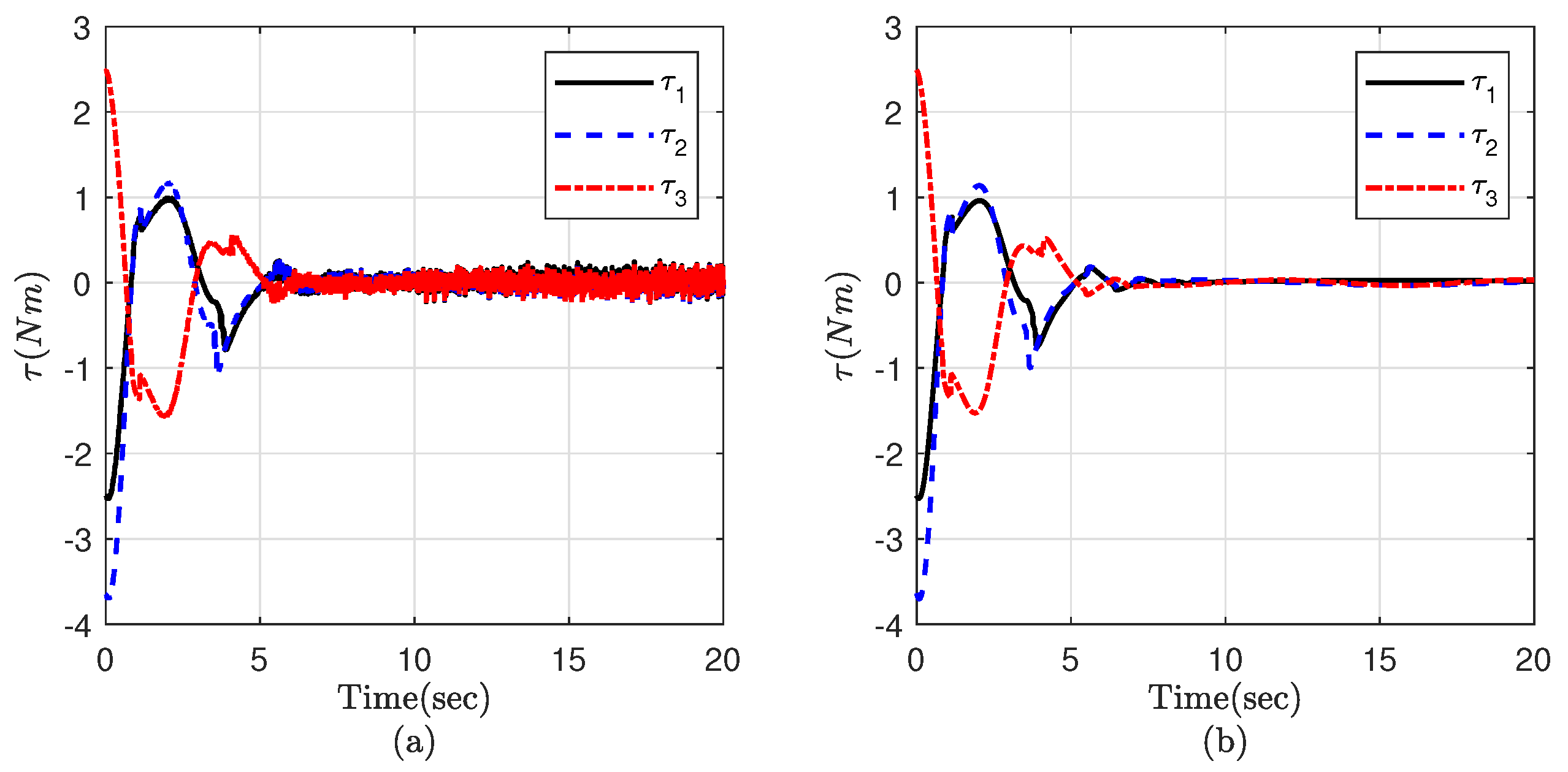
5. Simulation Results

This section aims at validating the performance of the suggested constrained control framework through conducting numerical simulations on a rigid spacecraft. In order to have a thorough evaluation, the simulation results are presented in three parts. The inertia matrix is not completely known and its nominal and uncertain parts are as ${\mathit{J}}_0=[20,1.2,0.9;1.2,17,1.4;0.9,1.4,15]$ kg m${}^2$ and $\Delta \mathit{J}=\mathrm{diag}(2,2,3)$ kg m${}^2$, respectively [53]. The space disturbance is taken as $\mathit{d}={2(\parallel \mathit{\omega }\parallel }^2{+0.3)[cos\left(0.2t\right),sin\left(0.5t\right),cos\left(0.8t\right)]}^T$ [53].

Part 1: Here, we consider four distinct initial states to see if the settling time depends upon the initial state. Based on the claim given in Theorem 1, it is expected that the state trajectories are driven to the origin before $T_c=T_{c1}+T_{c2}$. The four initial states are: (1) $\mathit{\sigma }\left(0\right)={[0.3,0.4,-0.3]}^T$, $\mathit{\omega }\left(0\right)={[-0.01,-0.01,0]}^T$ rad/sec, (2) $\mathit{\sigma }\left(0\right)={[-0.2,-0.1,0.3]}^T$, $\mathit{\omega }\left(0\right)={[0.01,0,-0.01]}^T$ rad/sec, 3) $\mathit{\sigma }\left(0\right)=[-0.6,0.45,$${-0.45]}^T$, $\mathit{\omega }\left(0\right)={[-0.01,0.01,-0.01]}^T$ rad/sec, 4) $\mathit{\sigma }\left(0\right)$$={[0.45,-0.6,0.6]}^T$, $\mathit{\omega }\left(0\right)={[0.08,0.08,-0.08]}^T$ rad/sec. The parameters of the controller (21), the adaptive update law (23), and the FTPPF (10) are selected as: ${\eta }_1={\eta }_2=5/9$, $T_{c1}=T_{c2}=5$, $\alpha =1$$\nu =0.2$, $g_1=0.1$, $g_2=0.1$, $g_3=0.2$, $g_4=-0.1$, $l=1$, $k_1=0.1$, $\vartheta =0.25$, ${\rho }_0=1$, $c_1=0.3$, ${\rho }_T=0.005$, and $T_f=10$.

The simulation results related this case are presented in Figure 4, Figure 5, Figure 6, Figure 7, Figure 8, Figure 9, Figure 10 and Figure 11. As it is observed in Figure 4 and Figure 6, the attitude and rotation velocity trajectories have converged before 10 seconds, that is, the summation of $T_{c1}$ and $T_{c2}$. The convergence time of the FTPPF (10), i.e., $T_f$ is also chosen as 10 seconds. Based on Figure 4, the prescribed performance for the attitude variable is obtained irrespective of the initial conditions. The steady state behaviors of the attitude and the rotation velocity are provided in Figure 5 and Figure 7, respectively. As can be observed, the attitude trajectories enter the convergence region before $t=10$ sec and stay thereafter which confirms the claim given in this paper. Based on Figure 8, it is vivid that if the spacecraft attitude trajectory moves toward the performance function $(\mathrm{i}.\mathrm{e}.,x_1\to \rho )$, the function $\kappa$ goes toward one. Then, the tan and $\lambda$ functions increase. Therefore, the $\gamma$ function, illustrated in Figure 9, rises since it is the integral of $\lambda$. To further evaluate this fact, see these two parameters associated with the first axis for the third initial condition, i.e., ${\lambda }_1$ and ${\gamma }_1$. It can be clearly seen that when the $x_{1i}$ goes towards the FTPPF $\rho$, the gain ${\lambda }_1$ rapidly goes up and there is a growth in ${\gamma }_1$ as well. However, when the attitude variable $x_{1i}$ changes its direction and moves to zero, the gain ${\lambda }_1$ begins to decline but it is still positive due to its definition. Hence, the gain ${\gamma }_1$ remains almost constant and it experiences a quite gradual increase. From Figure 10, when the distance between the attitude trajectory and the boundary of the constraint region is decreasing, the control effort is rising to preclude the attitude trajectory from violating the constraint. This is due to fact that the time-varying gains $\lambda$ and $\gamma$ proportionally appear in the control law (21) and their increase can lead to a growth in the control input. The steady state behaviors of the control torque is provided in Figure 11. It can be observed that the control input does not experience any chattering.

Part 2: In the previous part, the effect of different initial conditions on the time response of the attitude variable was investigated. Based on the definition ${\lambda }_i=tan\left(\frac{\pi {\kappa }_i}{2}\right)$ where ${\kappa }_i\left(t\right)=|\frac{{\mathit{\sigma }}_i\left(t\right)}{{\rho }_i\left(t\right)}{|}^{\vartheta }$, it is observed that the parameter $\vartheta$ plays an important role in the value of the time-varying gain ${\lambda }_i\left(t\right)$. Therefore, the impact of this parameter is evaluated in this part. The initial condition is taken as $\mathit{\sigma }\left(0\right)={[-0.2,-0.1,0.3]}^T$, and $\mathit{\omega }\left(0\right)={[1,0,-1]}^T$. The parameters of the controller, the update law, and the FTPPF are the same as in the previous part except for $\vartheta$. Here, various values for $\vartheta$ are considered as (1) $\vartheta =0.1$, (2) $\vartheta =0.2$, (3) $\vartheta =0.4$, and (4) $\vartheta =0.6$.

The simulation results are depicted in Figure 12, Figure 13 and Figure 14. It is clear that the attitude trajectory can be closer to the boundary of the permitted region if the parameter $\vartheta$ is not too small. The reason behind this fact is that if the initial value of the attitude attitude satisfies $|{\sigma }_i\left(0\right)|<{\rho }_i\left(0\right)$, then we have $\left|\frac{{\sigma }_i}{{\rho }_i}\right|<1$. Hence, for the same value of ${\sigma }_i$, a smaller $\vartheta$ results in a bigger ${\kappa }_i$. Therefore, ${\kappa }_i$ is closer to 1 and the time-varying gain ${\lambda }_i$ becomes bigger in this case and the system trajectory is not allowed to become close to the boundary of the FTPPF.

Part 3: The main objective of this part is to evaluate robustness of the proposed control scheme with respect to time-varying disturbances including high and low frequencies and measurement noises. To this end, it is supposed that the space disturbance is $\mathit{d}={2(\parallel \mathit{\omega }\parallel }^2{+0.3)[cos\left(0.2t\right),sin\left(0.5t\right),cos\left(0.8t\right)]}^T+[sin\left(200\pi t\right),sin\left(200\pi t\right),sin\left(200\pi t\right)]$${}^T$ [54]. As can be seen, the disturbance is composed of low- and high-frequency signals. Moreover, additive states noise with a standard deviation ${\mathit{\sigma }}_n$ is added to the attitude and angular velocity before measurement to produce noisy measurements. Given the measurement vectors, the noise is added in the form of white Gaussian noise with zero mean and standard deviation ${\mathit{\sigma }}_n$ [55]. The simulation results have been provided in Figure 15, Figure 16, Figure 17, Figure 18 and Figure 19. More specifically, Figure 15 and Figure 17 show that the attitude and angular velocity are stabilized in the presence of measurement noise and high-frequency disturbance. Looking at the time response of the attitude and angular velocity in Figure 16 and Figure 18, it is observed that the constraint imposed on the attitude is still satisfied and the proposed control scheme shows a satisfying performance with respect to measurement noise and high-frequency disturbance. Figure 19 presents the control torque. It is observed that the maximum required control torque is still in the acceptable range, but it shows some oscillations to suppress the negative effect of the measurement noise.

6. Conclusions

The problem of adaptive fixed-time attitude control with prescribed performance for rigid spacecraft subject to uncertainty and disturbance is studied in the present work. An important advantage of the proposed control scheme is that the smallest upper bound of the convergence time of the closed-loop attitude system is determined via an independent parameter which explicitly appears in the controller. Further, based on the concept of the funnel control for nonlinear systems, a time-varying gain is introduced to handle the constraints imposed on the spacecraft attitude. Thus, the controller structure is relatively simple since it contains no complicated terms to constrain the attitude variable. Moreover, it is confirmed that the system trajectories converge to arbitrary small region around the origin in a fixed time. Several simulations are conducted so as to support the presented theoretical results.

References

1. Zheng, M.; Wu, Y.; Li, C. Reinforcement learning strategy for spacecraft attitude hyperagile tracking control with uncertainties. Aerosp. Sci. Technol. 2021, 119, 107126. [Google Scholar] [CrossRef]
2. Yao, Q.; Jahanshahi, H.; Bekiros, S.; Mihalache, S.F.; Alotaibi, N.D. Indirect Neural-Enhanced Integral Sliding Mode Control for Finite-Time Fault-Tolerant Attitude Tracking of Spacecraft. Mathematics 2022, 10, 2467. [Google Scholar] [CrossRef]
3. Dai, M.Z.; Xiao, B.; Zhang, C.; Wu, J. Event-triggered policy to spacecraft attitude stabilization with actuator output nonlinearities. IEEE Trans. Circuits Syst. II Express Briefs 2021, 68, 2855–2859. [Google Scholar] [CrossRef]
4. Yao, Q. Robust attitude tracking control of spacecraft under unified actuator dynamics. Int. J. Control 2022. [Google Scholar] [CrossRef]
5. Show, L.L.; Juang, J.C.; Lin, C.T.; Jan, Y.W. Spacecraft robust attitude tracking design: PID control approach. In Proceedings of the 2002 American Control Conference (IEEE Cat. No. CH37301), Anchorage, AK, USA, 8–10 May 2002; Volume 2, pp. 1360–1365. [Google Scholar]
6. Najafizadeh Sari, N.; Jahanshahi, H.; Fakoor, M. Adaptive fuzzy PID control strategy for spacecraft attitude control. Int. J. Fuzzy Syst. 2019, 21, 769–781. [Google Scholar] [CrossRef]
7. Guo, Z.; Wang, Z.; Li, S. Global finite-time set stabilization of spacecraft attitude with disturbances using second-order sliding mode control. Nonlinear Dyn. 2022, 108, 1305–1318. [Google Scholar] [CrossRef]
8. Xia, Y.; Zhu, Z.; Fu, M.; Wang, S. Attitude tracking of rigid spacecraft with bounded disturbances. IEEE Trans. Ind. Electron. 2010, 58, 647–659. [Google Scholar] [CrossRef]
9. Sun, L.; Zheng, Z. Disturbance-observer-based robust backstepping attitude stabilization of spacecraft under input saturation and measurement uncertainty. IEEE Trans. Ind. Electron. 2017, 64, 7994–8002. [Google Scholar] [CrossRef]
10. Giuseppi, A.; Pietrabissa, A.; Cilione, S.; Galvagni, L. Feedback linearization-based satellite attitude control with a life-support device without communications. Control Eng. Pract. 2019, 90, 221–230. [Google Scholar] [CrossRef]
11. Seo, D.; Akella, M.R. High-performance spacecraft adaptive attitude-tracking control through attracting-manifold design. J. Guid. Control Dyn. 2008, 31, 884–891. [Google Scholar] [CrossRef]
12. Zhang, C.; Xiao, B.; Wu, J.; Li, B. On low-complexity control design to spacecraft attitude stabilization: An online-learning approach. Aerosp. Sci. Technol. 2021, 110, 106441. [Google Scholar] [CrossRef]
13. Lee, D. Fault-tolerant finite-time controller for attitude tracking of rigid spacecraft using intermediate quaternion. IEEE Trans. Aerosp. Electron. Syst. 2021, 57, 540–553. [Google Scholar] [CrossRef]
14. Huang, Y.; Jia, Y. Adaptive finite-time 6-DOF tracking control for spacecraft fly around with input saturation and state constraints. IEEE Trans. Aerosp. Electron. Syst. 2019, 55, 3259–3272. [Google Scholar] [CrossRef]
15. Lv, M.; Li, Y.; Pan, W.; Baldi, S. Finite-time fuzzy adaptive constrained tracking control for hypersonic flight vehicles with singularity-free switching. IEEE/ASME Trans. Mechatron. 2022, 27, 1594–1605. [Google Scholar] [CrossRef]
16. Yu, L.; Ye, D.; Sun, Z. Finite-time resilient attitude coordination control for multiple rigid spacecraft with communication link faults. Aerosp. Sci. Technol. 2021, 111, 106560. [Google Scholar] [CrossRef]
17. Najafi, A.; Vu, M.T.; Mobayen, S.; Asad, J.H.; Fekih, A. Adaptive barrier fast terminal sliding mode actuator fault tolerant control approach for quadrotor UAVs. Mathematics 2022, 10, 3009. [Google Scholar] [CrossRef]
18. Saghafi Zanjani, M.; Mobayen, S. Anti-sway control of offshore crane on surface vessel using global sliding mode control. Int. J. Control 2022, 95, 2267–2278. [Google Scholar] [CrossRef]
19. Mobayen, S.; Bayat, F.; ud Din, S.; Vu, M.T. Barrier function-based adaptive nonsingular terminal sliding mode control technique for a class of disturbed nonlinear systems. ISA Trans. 2022. [Google Scholar] [CrossRef]
20. Polyakov, A. Nonlinear feedback design for fixed-time stabilization of linear control systems. IEEE Trans. Autom. Control 2011, 57, 2106–2110. [Google Scholar] [CrossRef] [Green Version]
21. Xu, C.; Wu, B.; Wang, D.; Zhang, Y. Distributed fixed-time output-feedback attitude consensus control for multiple spacecraft. IEEE Trans. Aerosp. Electron. Syst. 2020, 56, 4779–4795. [Google Scholar] [CrossRef]
22. Aly, A.A.; The Vu, M.; El-Sousy, F.F.; Alotaibi, A.; Mousa, G.; Le, D.N.; Mobayen, S. Fuzzy-Based Fixed-Time Nonsingular Tracker of Exoskeleton Robots for Disabilities Using Sliding Mode State Observer. Mathematics 2022, 10, 3147. [Google Scholar] [CrossRef]
23. Du, H.; Zhang, J.; Wu, D.; Zhu, W.; Li, H.; Chu, Z. Fixed-time attitude stabilization for a rigid spacecraft. ISA Trans. 2020, 98, 263–270. [Google Scholar] [CrossRef] [PubMed]
24. Chen, Q.; Xie, S.; Sun, M.; He, X. Adaptive nonsingular fixed-time attitude stabilization of uncertain spacecraft. IEEE Trans. Aerosp. Electron. Syst. 2018, 54, 2937–2950. [Google Scholar] [CrossRef]
25. Zou, A.M.; Fan, Z. Distributed fixed-time attitude coordination control for multiple rigid spacecraft. Int. J. Robust Nonlinear Control 2020, 30, 266–281. [Google Scholar] [CrossRef]
26. Tao, M.; Chen, Q.; He, X.; Sun, M. Adaptive fixed-time fault-tolerant control for rigid spacecraft using a double power reaching law. Int. J. Robust Nonlinear Control 2019, 29, 4022–4040. [Google Scholar] [CrossRef]
27. Xiao, B.; Wu, X.; Cao, L.; Hu, X. Prescribed Time Attitude Tracking Control of Spacecraft with Arbitrary Disturbance. IEEE Trans. Aerosp. Electron. Syst. 2022, 58, 2531–2540. [Google Scholar] [CrossRef]
28. Cao, L.; Xiao, B.; Golestani, M. Robust fixed-time attitude stabilization control of flexible spacecraft with actuator uncertainty. Nonlinear Dyn. 2020, 100, 2505–2519. [Google Scholar] [CrossRef]
29. Cao, L.; Xiao, B.; Golestani, M.; Ran, D. Faster fixed-time control of flexible spacecraft attitude stabilization. IEEE Trans. Ind. Inform. 2020, 16, 1281–1290. [Google Scholar] [CrossRef]
30. Zuo, Z. Nonsingular fixed-time consensus tracking for second-order multi-agent networks. Automatica 2015, 54, 305–309. [Google Scholar] [CrossRef]
31. Chen, Q.; Xie, S.; He, X. Neural-network-based adaptive singularity-free fixed-time attitude tracking control for spacecrafts. IEEE Trans. Cybern. 2021, 51, 5032–5045. [Google Scholar] [CrossRef]
32. Yao, Q.; Jahanshahi, H.; Moroz, I.; Alotaibi, N.D.; Bekiros, S. Neural Adaptive Fixed-Time Attitude Stabilization and Vibration Suppression of Flexible Spacecraft. Mathematics 2022, 10, 1667. [Google Scholar] [CrossRef]
33. Bechlioulis, C.P.; Rovithakis, G.A. Robust adaptive control of feedback linearizable MIMO nonlinear systems with prescribed performance. IEEE Trans. Autom. Control 2008, 53, 2090–2099. [Google Scholar] [CrossRef]
34. Berger, T.; Lê, H.H.; Reis, T. Funnel control for nonlinear systems with known strict relative degree. Automatica 2018, 87, 345–357. [Google Scholar] [CrossRef]
35. Wei, C.; Chen, Q.; Liu, J.; Yin, Z.; Luo, J. An overview of prescribed performance control and its application to spacecraft attitude system. Proc. Inst. Mech. Eng. Part I J. Syst. Control Eng. 2021, 235, 435–447. [Google Scholar] [CrossRef]
36. Golestani, M.; Zhang, W.; Yang, Y.; Xuan-Mung, N. Disturbance observer-based constrained attitude control for flexible spacecraft. IEEE Trans. Aerosp. Electron. Syst. 2022. [Google Scholar] [CrossRef]
37. Wei, C.; Luo, J.; Dai, H.; Duan, G. Learning-based adaptive attitude control of spacecraft formation with guaranteed prescribed performance. IEEE Trans. Cybern. 2018, 49, 4004–4016. [Google Scholar] [CrossRef]
38. Gao, S.; Liu, X.; Jing, Y.; Dimirovski, G.M. Finite-time prescribed performance control for spacecraft attitude tracking. IEEE/ASME Trans. Mechatron. 2022, 27, 3087–3098. [Google Scholar] [CrossRef]
39. Gao, S.; Liu, X.; Jing, Y.; Dimirovski, G.M. A novel finite-time prescribed performance control scheme for spacecraft attitude tracking. Aerosp. Sci. Technol. 2021, 118, 107044. [Google Scholar] [CrossRef]
40. Fu, J.; Liu, M.; Cao, X.; Li, A. Robust neural-network-based quasi-sliding-mode control for spacecraft-attitude maneuvering with prescribed performance. Aerosp. Sci. Technol. 2021, 112, 106667. [Google Scholar] [CrossRef]
41. Munoz-Vazquez, A.J.; Sánchez-Torres, J.D.; Jimenez-Rodriguez, E.; Loukianov, A.G. Predefined-time robust stabilization of robotic manipulators. IEEE/ASME Trans. Mechatron. 2019, 24, 1033–1040. [Google Scholar] [CrossRef]
42. Xie, S.; Chen, Q. Adaptive nonsingular predefined-time control for attitude stabilization of rigid spacecrafts. IEEE Trans. Circuits Syst. II Express Briefs 2022, 69, 189–193. [Google Scholar] [CrossRef]
43. Sun, Y.; Zhang, L. Fixed-time adaptive fuzzy control for uncertain strict feedback switched systems. Inf. Sci. 2021, 546, 742–752. [Google Scholar] [CrossRef]
44. Golestani, M.; Esmailzadeh, M.; Mobayen, S. Constrained attitude control for flexible spacecraft: Attitude pointing accuracy and pointing stability improvement. IEEE Trans. Syst. Man Cybern. Syst. 2022. [Google Scholar] [CrossRef]
45. Mei, Y.; Wang, J.; Park, J.H.; Shi, K.; Shen, H. Adaptive fixed-time control for nonlinear systems against time-varying actuator faults. Nonlinear Dyn. 2022, 107, 3629–3640. [Google Scholar] [CrossRef]
46. Chen, Q.; Ren, X.; Na, J.; Zheng, D. Adaptive robust finite-time neural control of uncertain PMSM servo system with nonlinear dead zone. Neural Comput. Appl. 2017, 28, 3725–3736. [Google Scholar] [CrossRef]
47. Jin, X. Adaptive fixed-time control for MIMO nonlinear systems with asymmetric output constraints using universal barrier functions. IEEE Trans. Autom. Control 2019, 64, 3046–3053. [Google Scholar] [CrossRef]
48. Huang, Y.; Jia, Y. Adaptive fixed-time six-DOF tracking control for noncooperative spacecraft fly-around mission. IEEE Trans. Control Syst. Technol. 2019, 27, 1796–1804. [Google Scholar] [CrossRef]
49. Su, Y.; Zheng, C.; Mercorelli, P. Robust approximate fixed-time tracking control for uncertain robot manipulators. Mech. Syst. Signal Process. 2020, 135, 106379. [Google Scholar] [CrossRef]
50. Guo, B.Z.; Zhao, Z.L. On convergence of the nonlinear active disturbance rejection control for MIMO systems. SIAM J. Control Optim. 2013, 51, 1727–1757. [Google Scholar] [CrossRef]
51. Beltran-Carbajal, F.; Valderrabano-Gonzalez, A.; Favela-Contreras, A.R.; Rosas-Caro, J.C. Active disturbance rejection control of a magnetic suspension system. Asian J. Control 2015, 17, 842–854. [Google Scholar] [CrossRef]
52. Khalil, H.K.; Praly, L. High-gain observers in nonlinear feedback control. Int. J. Robust Nonlinear Control 2014, 24, 993–1015. [Google Scholar] [CrossRef]
53. Lu, K.; Xia, Y. Adaptive attitude tracking control for rigid spacecraft with finite-time convergence. Automatica 2013, 49, 3591–3599. [Google Scholar] [CrossRef]
54. Yu, S.; Yu, X.; Shirinzadeh, B.; Man, Z. Continuous finite-time control for robotic manipulators with terminal sliding mode. Automatica 2005, 41, 1957–1964. [Google Scholar] [CrossRef]
55. Rahimi, A.; Kumar, K.D.; Alighanbari, H. Fault detection and isolation of control moment gyros for satellite attitude control subsystem. Mech. Syst. Signal Process. 2020, 135, 106419. [Google Scholar] [CrossRef]
Figure 1. Coordinate reference frames. [28].
Mathematics 11 00247 g001
Figure 2. Comparison of | x | 0.7 sgn ( x ) and x, sgn ( x ) , and | x | .
Mathematics 11 00247 g002
Figure 3. The diagram of the novel NN-based control for the rigid spacecraft attitude system.
Mathematics 11 00247 g003
Figure 4. Time responses of the attitude in Part 1 for different initial conditions.
Mathematics 11 00247 g004
Figure 5. Steady state behavior of the attitude in Part 1 for different initial conditions.
Mathematics 11 00247 g005
Figure 6. Time responses of the rotation velocity in Part 1 for different initial conditions.
Mathematics 11 00247 g006
Figure 7. Steady state behavior of the rotation velocity in Part 1 for different initial conditions.
Mathematics 11 00247 g007
Figure 8. The parameter λ in Part 1 for different initial conditions.
Mathematics 11 00247 g008
Figure 9. The parameter γ in Part 1 for different initial conditions.
Mathematics 11 00247 g009
Figure 10. The control torque in Part 1 for different initial conditions.
Mathematics 11 00247 g010
Figure 11. Steady state behavior of the control torque in Part 1 for different initial conditions.
Mathematics 11 00247 g011
Figure 12. Time responses of the attitude in Part 2 for different ϑ .
Mathematics 11 00247 g012
Figure 13. Time responses of the rotation velocity in Part 2 for different ϑ .
Mathematics 11 00247 g013
Figure 14. The control torque in Part 2 for different ϑ .
Mathematics 11 00247 g014
Figure 15. The attitude in Part 3: (a) noisy measurement, (b) high-frequency disturbance.
Mathematics 11 00247 g015
Figure 16. The attitude in Part 3 in steady state: (a) noisy measurement, (b) high-frequency disturbance.
Mathematics 11 00247 g016
Figure 17. The rotation velocity in Part 3: (a) noisy measurement, (b) high-frequency disturbance.
Mathematics 11 00247 g017
Figure 18. The rotation velocity in Part 3 in steady state: (a) noisy measurement, (b) high-frequency disturbance.
Mathematics 11 00247 g018
Figure 19. The control torque in Part 3: (a) noisy measurement, (b) high-frequency disturbance.
Mathematics 11 00247 g019
Disclaimer/Publisher’s Note: The statements, opinions and data contained in all publications are solely those of the individual author(s) and contributor(s) and not of MDPI and/or the editor(s). MDPI and/or the editor(s) disclaim responsibility for any injury to people or property resulting from any ideas, methods, instructions or products referred to in the content.