Article

Scalar Field Cosmology from a Modified Poisson Algebra

by
Genly Leon
1,2,*,
Alfredo D. Millano
1 and
Andronikos Paliathanasis
1,2
1
Departamento de Matemáticas, Universidad Católica del Norte, Avda. Angamos 0610, Casilla 1280, Antofagasta 1240000, Chile
2
Institute of Systems Science, Durban University of Technology, Durban 4000, South Africa
*
Author to whom correspondence should be addressed.
Mathematics 2023, 11(1), 120; https://doi.org/10.3390/math11010120
Submission received: 6 December 2022 / Revised: 22 December 2022 / Accepted: 24 December 2022 / Published: 27 December 2022
(This article belongs to the Special Issue Noncommutativity, Gravity and Cosmology)

Abstract

:
We investigate the phase space of a scalar field theory obtained by minisuperspace deformation. We consider quintessence or phantom scalar fields in the action that arises from minisuperspace deformation on the Einstein–Hilbert action. We use a modified Poisson algebra where Poisson brackets are the α -deformed ones and are related to the Moyal–Weyl star product. We discuss early- and late-time attractors and reconstruct the cosmological evolution. We show that the model can have the ΛCDM model as a future attractor if we initially consider a massless scalar field without a cosmological constant term.
PACS:
98.80.-k; 95.35.+d; 95.36.+x
MSC:
83D05; 17B63; 37J25; 37J39

1. Introduction

Cosmological observations indicate that the universe has gone through two acceleration phases [1,2,3,4], an early acceleration phase known as inflation and the present acceleration phase. The source of the cosmic acceleration is unknown. In the context of General Relativity, cosmic acceleration occurs when the cosmic fluid is dominated by a vacuum-like source known as dark energy (DE) with the property of having a negative value of the equation of state (EoS) parameter.
The cosmological constant Λ leads to the Λ -cosmology being indeed the simplest candidate for DE; however, it suffers from two problems, the fine-tuning and the coincidence problems [5,6]. Furthermore, the detailed analysis of the recent cosmological observations shows that the Λ -cosmology cannot solve tensions arising from the statistical analysis of the data, such as the H 0 -tension [7]. There are various DE alternatives to the cosmological constant, which have been proposed to overpass the above-mentioned problems; see, for instance [8,9,10,11,12,13,14,15,16,17] and the references therein.
Scalar fields play a significant role in the description of cosmic acceleration. Indeed, introducing a scalar field in the field equations provides new degrees of freedom in the gravitational dynamics that provide acceleration effects. The most straightforward mechanism for describing the early acceleration phase of the universe, that is of the inflationary epoch, is that of the inflaton field [18,19,20,21,22,23,24,25]. During inflation [26,27], the scalar field dominates the cosmological dynamics and provides the antigravity effects. Similarly, for the description of the late-time acceleration [28], a tracker scalar field can be introduced [12], which roles down the potential energy V ( ϕ ) to have DE effects [29,30,31,32,33]. Another novelty of the scalar fields is that they can reproduce various DE alternatives such as the Chaplygin gas and others [34,35].
In quintessence scalar field cosmology [8], the EoS parameter of the scalar field is constrained to the range w ϕ 1 , where w ϕ = 1 corresponds to a stiff fluid, where only the kinetic part of the scalar field dominates, while the limit w ϕ = 1 corresponds to the case where only the scalar field potential dominates, leading to the Λ -cosmology. Recall that acceleration occurs when 1 w e f f < 1 / 3 . There is a family of scalar field models, known as phantom scalar fields, where w ϕ can cross the limit 1 and take smaller values, which is possible, for example, when there exists a negative kinetic energy [36,37,38,39].
During the very early stages of the universe, we expect that quantum effects play an important role in cosmic evolution. Until now, there is not a unique theory of quantum gravity; that is why various approaches have been considered in the literature by various groups [40,41,42,43,44,45,46,47,48]. String theory, double-special relativity, and the generalized uncertainty principle require the existence of a minimum length scale of the order of the Planck length l pl [49,50,51,52,53,54,55,56]. As a result of the modification of the Heisenberg uncertainty in the latter approaches, a deformation parameter is introduced, which leads to the deformation of the coordinate representation of the operators of the momentum position, that is to a deformation of the Poisson algebra [57].
Noncommutative theories, quantum cosmology, quantum deformation, deformed phase space, Brans–Dicke theory, and noncommutative minisuperspace, as alternatives of the cosmological constant, have been treated, for example, in [58,59,60,61,62,63,64] and the references therein.
In [65], the phase space for the cosmological dynamics in quintessence cosmology was modified by a deformed Poisson algebra among the coordinates and the canonical momenta. The main result was that the deformation parameter is related to the accelerating scale factor provided by the deformed Poisson algebra in the absence of a cosmological constant. A similar result was determined recently in [66] and the case of a phantom scalar field.
The Moyal–Weyl star product provides a simple prescription for constructing noncommutative field theories on the noncommutative manifold [65] with [ x ^ μ , x ^ ν ] = i θ μ ν . One replaces all the pointwise products in ordinary field theory with one of the star products. For example, the noncommutative action for a real massless scalar field Φ in four dimensions is
S ϕ = 1 2 d 4 x D μ Φ α D μ Φ ,
where the ordinary derivative μ appearing in the commutative scalar field action is replaced by the noncommutative covariant derivative D μ and the action is invariant under the noncommutative gauge transformation.
In this paper, we are interested in studying the effects of the deformed Poisson algebra in the cosmological evolution. Specifically, we perform a detailed phase space analysis to investigate the existence of equilibrium points and reconstruct the cosmological parameters’ evolution. Such an analysis provides important information about the theory’s viability and can give us important results for the nature of the deformation parameter. For this analysis, one can introduce auxiliary variables, which transform the cosmological equations into an autonomous dynamical system [67,68,69,70,71,72,73,74,75,76,77,78,79,80,81]. Hence, we obtain a system of the form X = f ( X ) , where X is the column vector of the auxiliary variables and f ( X ) is an autonomous vector field. The derivative is with respect to a logarithmic time scale. The stability analysis comprises several steps. First, the critical points X c are extracted under the requirement of X = 0 . Then, one considers linear perturbations around X c as X = X c + U , with U the column vector of the auxiliary variable’s perturbations. Therefore, up to first order, we obtain U = Ξ · U , where the matrix Ξ contains the coefficients of the perturbed equations. Finally, the type stability of each hyperbolic critical point is determined by the eigenvalues of Ξ . That is, the point is stable (unstable) if the real parts of the eigenvalues are negative (positive) or a saddle point if the eigenvalues have real parts with different signs.
The structure of the paper is as follows. In Section 2, we introduce the modified Poisson algebra. In Section 3, we derive the modified field equations in the case of scalar field cosmology in an isotropic and homogeneous spatially flat universe. Section 4 and Section 5 include the main results of this study, where we present the detailed analysis of the phase space for the modified field equations. Finally, in Section 6, we summarize our results and conclude.

2. Modified Poisson Algebra

We consider the modified Poisson algebra [65]:
{ x 1 , x j } α = θ i j ,
{ p i , p j } α = β i j ,
{ x i , p j } α = δ i j + σ i j ,
where the Moyal–Weyl brackets are defined through the relation:
{ f , g } α = f α g g α f
in which the product between f and g is substituted by the Moyal–Weyl star product:
( f α g ) = exp 1 2 α a b a ( 1 ) b ( 2 ) f ( x 1 ) g ( x 2 ) | x 1 = x 2 = x ,
such that
α = θ i j δ i j + σ i j δ i j σ i j β i j ,
where θ i j and β i j are 2 × 2 antisymmetric matrices indicating the noncommutativity in the coordinates and momenta, respectively. Particular deformations:
θ i j = θ ϵ i j , β i j = β ϵ i j ,
where ϵ i j is the two-index Levi-Civita symbol, are considered.
By removing the sub-index in α , the ★-Friedman equations can be derived for the ★-FLRW metric as follows [82].
R μ ν 1 2 R g μ ν + Λ g μ ν = κ T μ ν
with the energy–momentum tensor:
T μ ν = p g μ ν + ( ρ + p ) U μ U ν
where U μ = δ μ 0 is the co-moving observer and p and ρ are the total pressure and fluid energy three-density, respectively.
To avoid the complexities of ★-algebras, one may consider the field equations arising from the point-like action for a scalar field with action [83]:
S = d t N 3 a a ˙ 2 N 2 + 1 2 d t N a 3 ϵ ϕ ˙ 2 N 2 2 V ( ϕ ) .
We define the point-like Lagrangian [83]:
L ( N , a , ϕ , a ˙ , ϕ ˙ ) : = 1 N 3 a a ˙ 2 + 1 2 a 3 ϵ ϕ ˙ 2 a 3 N V ( ϕ ) ,
while, for simplicity, we consider a constant potential V ( ϕ ) = Λ ˜ . The sign ϵ = 1 corresponds to quintessence, and the sign ϵ = 1 corresponds to the phantom field.
With the variation with respect to { N , a , ϕ } and the replacement N = 1 after variation, we obtain the Euler–Lagrange equations:
1 2 6 a a ˙ 2 a 3 2 Λ ˜ + ϵ ϕ ˙ 2 = 0 ,
3 2 4 a a ¨ + 2 a ˙ 2 + a 2 ϵ ϕ ˙ 2 2 Λ ˜ = 0 ,
ϵ a 2 3 a ˙ ϕ ˙ + a ϕ ¨ = 0 .
Introducing the Hubble parameter H = a ˙ / a , the previous equations can be written as [83]:
3 H 2 = Λ ˜ + 1 2 ϵ ϕ ˙ 2 ,
2 H ˙ = 3 H 2 + Λ ˜ 1 2 ϵ ϕ ˙ 2 ,
ϕ ¨ + 3 H ϕ ˙ = 0 .
For the Lagrangian function (12), we define the generalized momenta by p i = L q ˙ i , where q i { a , ϕ } , p i { p a , p ϕ } , namely
p a 6 a a ˙ N , p ϕ ϵ a 3 ϕ ˙ N .
Hence, we can introduce the Hamiltonian function H = p a a ˙ + p ϕ ϕ ˙ L , which is written as
H = N p a 2 12 a + ϵ p ϕ 2 2 a 3 + Λ ˜ a 3
We define the canonical coordinates [83]:
x = λ 1 ( ϵ a ) 3 / 2 sinh ( ϵ λ ϕ ) , y = λ 1 a 3 / 2 cosh ( ϵ λ ϕ ) ,
with the inverse:
a = λ y 1 ϵ x 2 y 2 2 / 3 , ϕ = tanh 1 ϵ x / y λ ϵ ,
where λ 1 = 8 / 3 , and we consider the simpler case where the matter content is an ordinary ( ϵ = + 1 ) or a phantom ( ϵ = 1 ) scalar field in the action. Then, (12) becomes
L ( N , a , ϕ , a ˙ , ϕ ˙ ) : = 1 N 3 a a ˙ 2 + 1 2 a 3 ϵ ϕ ˙ 2 a 3 N V ( ϕ ) .
Generalized momenta are given by
P x = ϵ x ˙ N , P y = y ˙ N .
Hence, the problem can be formulated from the canonical Hamiltonian:
H c = ϵ N 1 2 P x 2 + ω 2 2 x 2 N 1 2 P y 2 + ω 2 2 y 2 ,
where ω 2 = 3 Λ ˜ / 4 , and we use the comoving frame N = 1 . For the choice ϵ = + 1 , see the related work [65].
We have the evolution equations for ( x ˙ , y ˙ ) as given by (24):
x ˙ = ϵ P x , y ˙ = P y
Hamilton’s equations p ˙ i = H q i , where H = H c and q i { x , y } , p i { P x , P y } , lead to
P x ˙ = ϵ ω 2 x , P y ˙ = ω 2 y .
which lead to the following equations for ϵ = ± 1 :
x ¨ + ω 2 x = 0 , y ¨ + ω 2 y = 0 ,
with conserved quantity:
y ˜ 2 ϵ x ˜ 2 = 1 , ( x ˜ , y ˜ ) = λ a 3 / 2 · ( x , y ) .
By the definition ω 2 = 3 / 4 Λ ˜ , the solutions are
x ( t ) = c 1 e 1 2 3 Λ ˜ t + c 2 e 1 2 3 Λ ˜ t ,
y ( t ) = c 3 e 1 2 3 Λ ˜ t + c 4 e 1 2 3 Λ ˜ t .
Then,
ϕ ( t ) = coth 1 ϵ 3 / 2 c 3 e 3 Λ ˜ t + c 4 c 1 e 3 Λ ˜ t + c 2 λ ϵ ,
a ( t ) = e Λ ˜ 3 t λ c 3 e 3 Λ ˜ t + c 4 2 / 3 1 ϵ c 1 e 3 Λ ˜ t + c 2 2 c 3 e 3 Λ ˜ t + c 4 2 1 / 3 ,
such that
ϕ ln 1 2 c 1 c 1 c 3 ϵ 3 / 2 2 λ ϵ , a c 3 2 / 3 λ 2 / 3 1 c 1 2 ϵ c 3 2 3 e Λ ˜ t 3
as t . That is, a de Sitter solution is obtained.
The elements of the new configuration space, ( x , y ) , and their conjugate momenta fulfil the following commutation relations based on the Poisson bracket:
{ x k , x j } = 0 , { P x k , P x j } = 0 , { x k , P x j } = δ k j
where k and j can take 1 and 2, that is ( x 1 , x 2 ) = ( x , y ) and δ k j is the usual Kronecker delta.
To obtain a modified scenario, we take classical phase space variables ( x , y , P x , P y ) and perform the transformation (see the related work [65]):
x ^ y ^ = x y + θ 2 P y P x
and
P ^ x P ^ y = β 2 y x + P x P y
The modified Poisson Algebra is given by
{ y ^ , x ^ } = θ , { P ^ y , P ^ x } = β
and
{ x ^ , P ^ x } = 1 + σ , { y ^ , P ^ y } = 1 + σ ,
where σ = θ β / 4 . Now, we change the notation { x ^ , y ^ , P ^ x , P ^ y } to { x , y , p x , p y } .
The modified Hamiltonian will be
H m o d . = 1 2 ϵ p x 2 1 2 p y 2 ω 1 2 2 x p y + ϵ y p x + ω 2 2 2 ( ϵ x 2 y 2 ) ,
where
p x = x ˙ + 1 2 ω 1 y , p y = x ω 1 2 ϵ 2 y ˙ 2 ϵ ,
and and we define the parameters
ω 1 2 = 4 β 4 ϵ ω 2 θ 4 ϵ ω 2 θ 2 , ω 2 2 = 4 ω 2 ϵ β 2 4 ϵ ω 2 θ 2 ,
Λ = 4 ( β 1 ) β ϵ + ( θ 4 ) ω 2 3 θ 2 ω 2 ϵ 4 .
If ω = 0 , the latter definitions are
ω 1 2 = β , ω 2 2 = ϵ β 2 4 , Λ = ( β 1 ) β ϵ 3 .
We can infer from these that the cosmological constant term is introduced from the modification of the Poisson algebra if our initial model does not include a cosmological constant term. The equations of motion derived from H m o d . are
x ¨ + ω 1 2 y ˙ 3 4 Λ x = 0 ,
and
y ¨ + ϵ ω 1 2 x ˙ 3 4 Λ y = 0 ,
These equations have the solutions:
x ( t ) = c 1 cosh t ω 1 2 2 cosh 1 2 t 3 Λ + ω 1 4 c 3 sinh t ω 1 2 2 cosh 1 2 t 3 Λ + ω 1 4
+ sinh 1 2 t 3 Λ + ω 1 4 c 3 ω 1 2 + 2 c 2 cosh t ω 1 2 2 c 1 ω 1 2 + 2 c 4 sinh t ω 1 2 2 3 Λ + ω 1 4 , y ( t ) = c 3 cosh t ω 1 2 2 cosh 1 2 t 3 Λ + ω 1 4 c 1 sinh t ω 1 2 2 cosh 1 2 t 3 Λ + ω 1 4
+ sinh 1 2 t 3 Λ + ω 1 4 c 1 ω 1 2 + 2 c 4 cosh t ω 1 2 2 c 3 ω 1 2 + 2 c 2 sinh t ω 1 2 2 3 Λ + ω 1 4 .
Some solutions of this form have been found before in the literature, e.g., [84,85].

3. Modified Friedmann Equations

Equations (45) and (46) are equivalent to
a ¨ = a ˙ 2 2 a 1 6 a 4 λ ϵ ϕ ˙ λ ϕ ˙ + ω 1 2 + 4 ω 2 2 + ω 1 2 ϵ ,
ϕ ¨ = 3 a ˙ 2 λ ϕ ˙ + ω 1 2 2 λ a
with the first integral
3 H 2 + 1 2 ϵ ϕ ˙ 2 4 ω 2 2 3 ω 1 2 ϵ 3 = 0 .
where H = a ˙ / a is the Hubble parameter.

3.1. Vacuum Case

Using the reparameterization (43), the modified Friedman equation reads
3 H 2 = 1 2 ϵ ϕ ˙ 2 + Λ .
The modified Klein–Gordon equation is
ϕ ¨ = H 6 ω 1 2 + 3 ϕ ˙
The Raychaudhuri equation is
H ˙ = 3 H 2 2 ϵ ω 1 2 ϕ ˙ 6 1 4 ϵ ϕ ˙ 2 + Λ 2 ,
Alternatively, by removing H 2 and using (52), we obtain
H ˙ = ϵ ω 1 2 ϕ ˙ 6 1 2 ϵ ϕ ˙ 2 .
With the definitions:
ρ ϕ = 1 2 ϵ ϕ ˙ 2 + Λ , P ϕ = 1 2 ϵ ϕ ˙ 2 + 2 3 ω 1 2 ϵ ϕ ˙ Λ ,
the Klein–Gordon equation can be written as the conservation equation:
ρ ˙ ϕ + 3 H ( ρ ϕ + P ϕ ) = 0 .
Moreover, we define the effective EoS parameter of ϕ as
w ϕ : = P ϕ ρ ϕ = ϵ ϕ ˙ 2 + 2 2 3 ω 1 2 ϵ ϕ ˙ 2 Λ ϵ ϕ ˙ 2 + 2 Λ .

3.2. Including Matter

The Friedman equation reads
3 H 2 = 1 2 ϵ ϕ ˙ 2 + ρ m + Λ .
The modified Klein–Gordon equation is
ϕ ¨ = H 6 ω 1 2 + 3 ϕ ˙
which can be written using (56) as
ρ ˙ ϕ + 3 H ( ρ ϕ + P ϕ ) = 0 .
We have the matter conservation equation:
ρ ˙ m + 3 H ( 1 + w m ) ρ m = 0 .
The Raychaudhuri equation is
H ˙ = ω 1 2 ϵ ϕ ˙ 6 1 2 ϵ ϕ ˙ 2 1 2 w m + 1 ρ m .

4. Dynamical Systems’ Analysis in the Vacuum Case

In this section, we proceed with the analysis of the phase space for the modified cosmological field equations. In order to perform such an analysis, we define dimensionless variables in the Hubble normalization approach, that is
Σ ϕ = ϕ ˙ 6 H , Σ = ω 1 2 H ,
which satisfies the constraint equation:
Σ ϕ 2 ϵ + μ Σ 2 = 1 ,
where we have introduced the constant μ = Λ / ( 3 ω 1 4 ) , or, alternatively,
Σ ϕ 2 ϵ + Ω Λ = 1 .
where, for convenience, we define the fractional energy density of Λ as
Ω Λ : = Λ 3 H 2 = μ Σ 2 , μ > 0 .
Thus, the dynamical system (52), (53), and (55) can be written as a dynamical system:
Σ ϕ = ( 3 Σ ϕ + Σ ) Σ ϕ 2 ϵ 1 ,
Σ = ϵ Σ ϕ Σ ( 3 Σ ϕ + Σ ) ,
where we have introduced the new time derivative f = H 1 f ˙ .

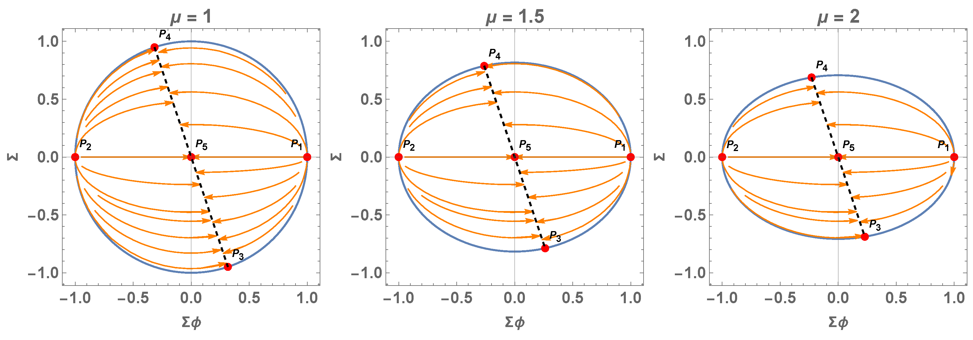
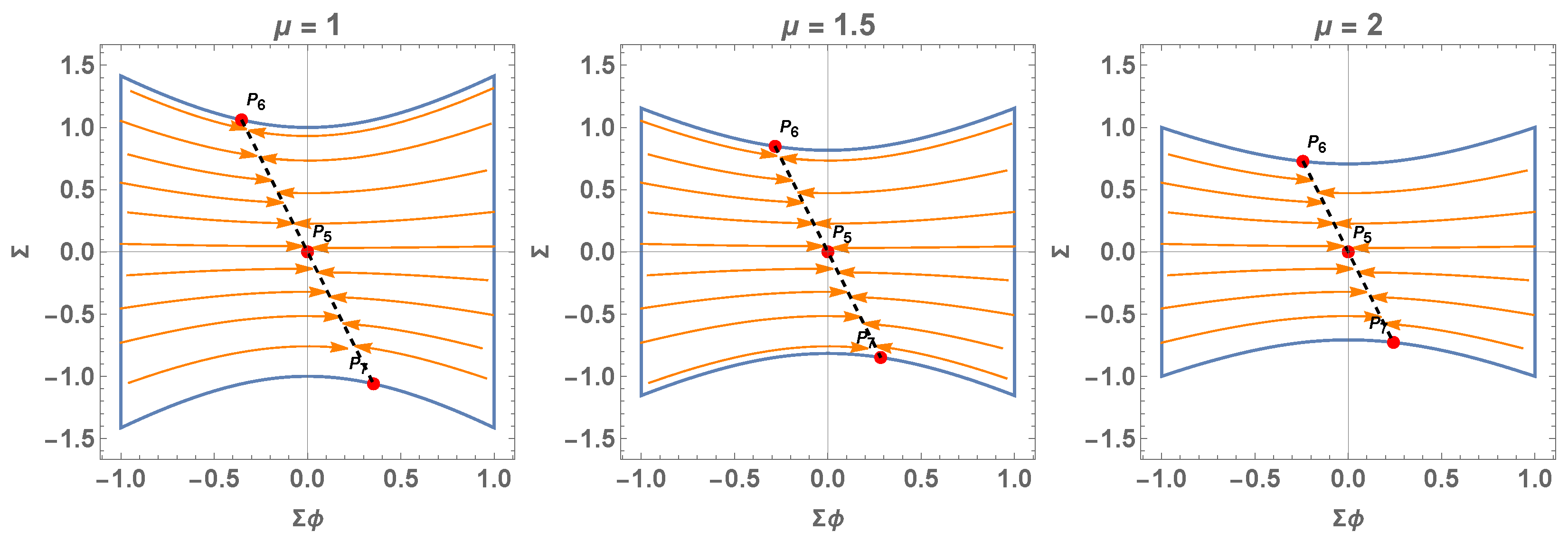
4.1. Analysis of the 2D Flow

In this section, we analyze the 2D flow associated with the dynamical system (68) and (69). We obtain the (lines of) equilibrium points of the system (68) and (69), which are summarized in Table 1 for ϵ = ± 1 along with with their coordinates, eigenvalues, and stability.

4.1.1. Case ϵ = + 1

In the case ϵ = + 1 , there exist kinetic-dominated solutions, given by the points P 1 and P 2 . They represent stiff solutions ( w ϕ = 1 ).
There is a line of equilibrium points L 1 , which corresponds to
ϕ ˙ + 6 3 ω 1 2 = 0 ϕ = 6 3 ω 1 2 t + c 1 .
Then, from (55), we have at the lines of the equilibrium points
H ˙ = 0 H = H 0 , a = e H 0 ( t t U ) .
where H 0 satisfies 3 H 0 2 = Λ + ω 1 4 ϵ 3 . That is a de Sitter solution.
Moreover, imposing the condition (65), the lines are reduced to the points P 3 and P 4 that belong to the lines of the equilibrium points 3 Σ ϕ + Σ = 0 .
For these equilibrium points, we have ϕ ˙ = 6 Σ ϕ 1 , 2 H , where Σ ϕ 1 , 2 = ± 1 / 9 μ + 1 . Hence,
H ˙ + Σ ϕ 1 , 2 H 3 Σ ϕ 1 , 2 H + Λ / ( 3 μ ) = 0 .
That is,
H = 3 H 0 Λ μ 9 H 0 Σ ϕ 1 , 2 + 3 Λ μ e ( t t U ) Σ ϕ 1 , 2 Λ 3 μ 9 H 0 Σ ϕ 1 , 2 .
The line L 1 also contains the point P 5 , which is a sink, but does not satisfy the condition (65).
Figure 1 presents a phase plot for System (68)–(69) for ϵ = + 1 and different values of μ . The dashed black line corresponds to L 1 .

4.1.2. Case ϵ = 1

For the case ϵ = 1 , the equilibrium points of the system (68) and (69) are, as before, the line L 1 , which contains P 5 (which does not satisfy (65). Moreover, imposing the condition (65), the lines are reduced to the points P 6 and P 7 that belong to the lines of equilibrium points 3 Σ ϕ + Σ = 0 , where Σ ϕ 1 , 2 = 1 / 9 μ 1 .
For these equilibrium points, we have ϕ ˙ = 6 Σ ϕ 1 , 2 H . Hence,
H ˙ Σ ϕ 1 , 2 H 3 Σ ϕ 1 , 2 H + Λ / ( 3 μ ) = 0 .
That is,
H = 3 H 0 Λ μ 9 H 0 Σ ϕ 1 , 2 + 3 Λ μ e ( t t U ) Σ ϕ 1 , 2 Λ 3 μ 9 H 0 Σ ϕ 1 , 2 .
Figure 2 presents a phase plot for System (68)–(69) for ϵ = 1 and different values of μ . The dashed black line corresponds to L 1 .

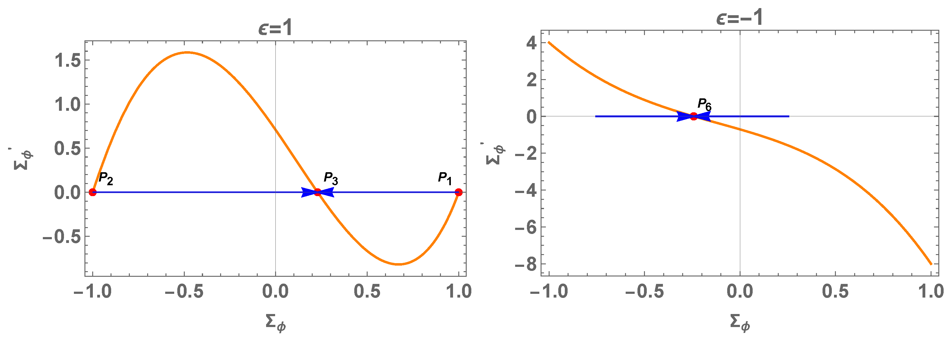
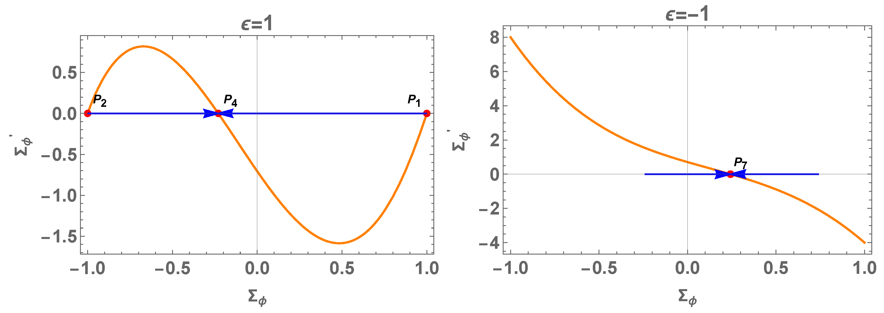
4.2. The 1D Reduced System

Using (65) to reduce the dimensionality and for Σ 0 , we have
Σ = ( 1 Σ ϕ 2 ϵ ) / μ .
Then, we have the reduced dynamical system:
Σ ϕ = 3 Σ ϕ + ( 1 Σ ϕ 2 ϵ ) / μ 1 Σ ϕ 2 ϵ ,
This patch covers only the equilibrium points (68)–(69) with Σ > 0 and Σ ϕ = 0 , say P 1 : Σ ϕ = 1 , P 2 : Σ ϕ = 1 and P 4 : Σ ϕ = 1 / 9 μ + 1 . Moreover, the equilibrium point of the 1D system (77) is P 6 : Σ ϕ = 1 / 9 μ 1 .
Table 2 presents the equilibrium points of System (77) for ϵ = ± 1 with their eigenvalues and stability.
Figure 3 presents a phase plot for the reduced 1D equation (77) for ϵ = ± 1 and μ = 2 .
On the other hand, using
Σ = ( 1 Σ ϕ 2 ϵ ) / μ ,
we have the reduced dynamical system:
Σ ϕ = 3 Σ ϕ ( 1 Σ ϕ 2 ϵ ) / μ 1 Σ ϕ 2 ϵ ,
This patch covers only the equilibrium points (68)–(69) with Σ < 0 and Σ ϕ = 0 , say P 1 : Σ ϕ = 1 , P 2 : Σ ϕ = 1 and P 3 : Σ ϕ : = 1 / 9 μ + 1 . Moreover, the equilibrium point of the 1D system (79) is P 7 : Σ ϕ = 1 / 9 μ 1 , which belongs to the lines of the equilibrium points 3 Σ ϕ + Σ = 0 .
Table 3 presents the equilibrium points of System (79) for ϵ = ± 1 with their eigenvalues and stability.
Figure 4 presents a phase plot for the reduced 1D equation (79) for ϵ = ± 1 and μ = 2 .

5. Dynamical Systems’ Analysis by Including Matter
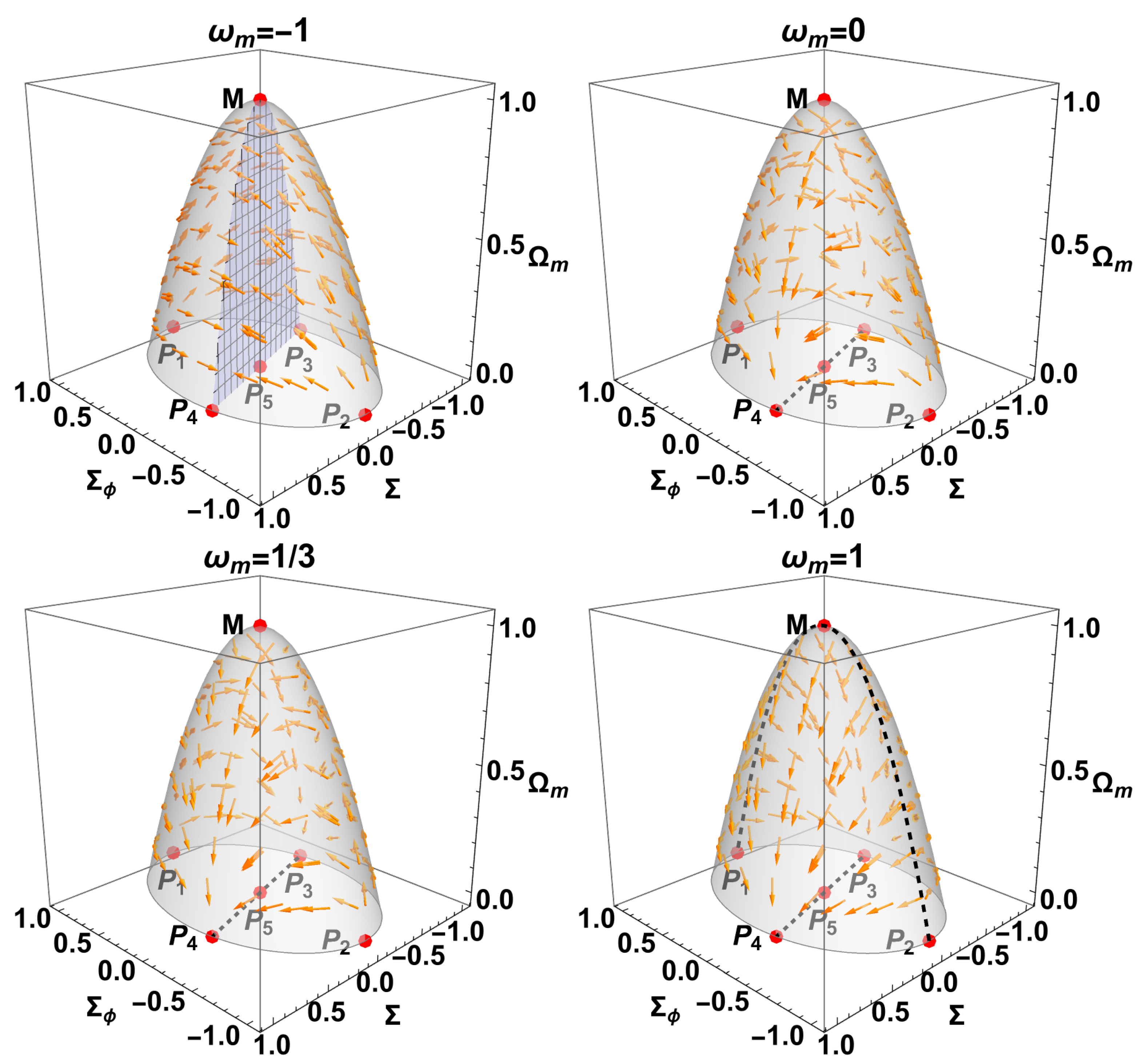
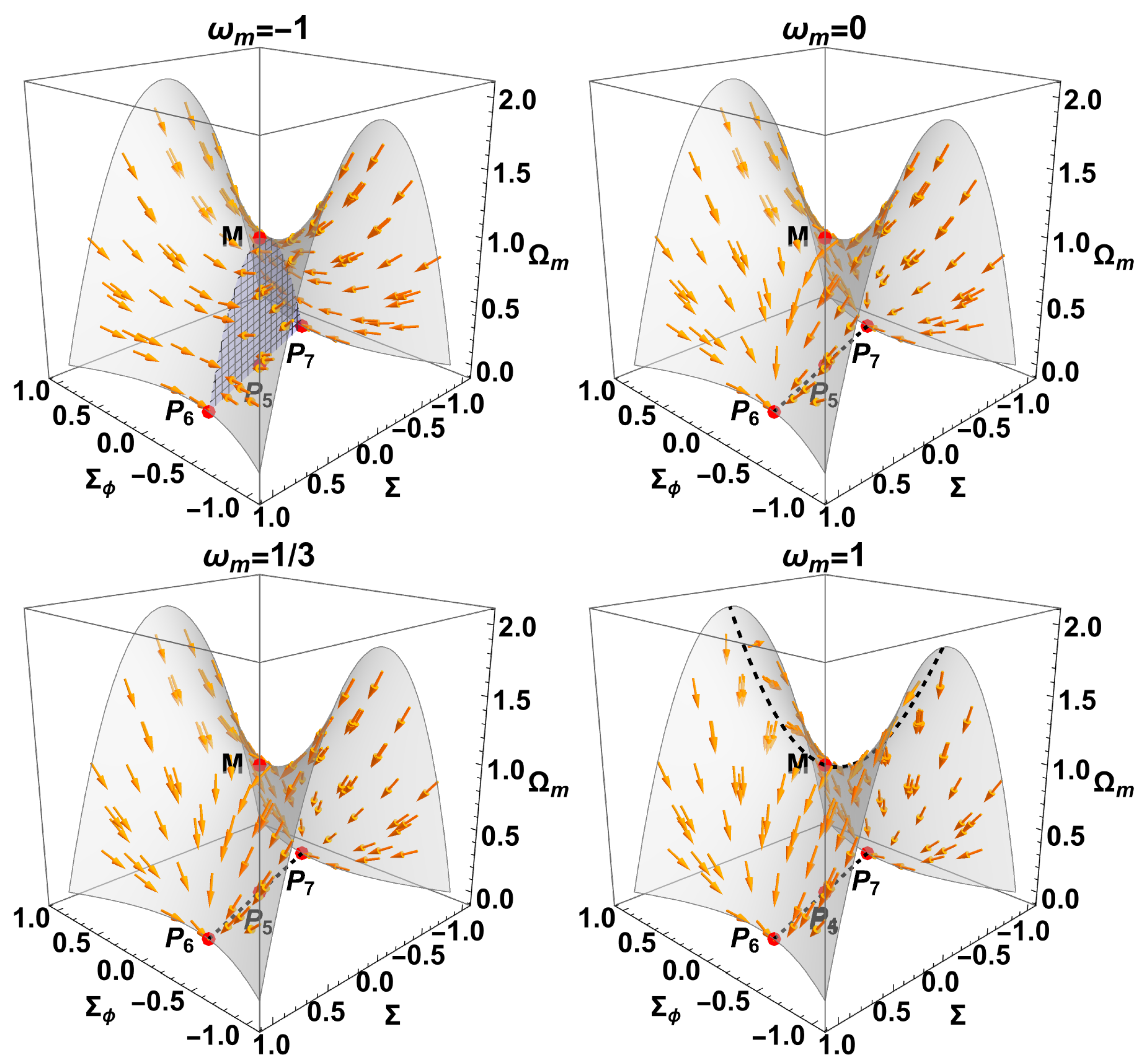
We define
Σ ϕ = ϕ ˙ 6 H , Σ = ω 1 2 H , Ω m = ρ m 3 H 2 ,
which satisfy
Σ ϕ 2 ϵ + μ Σ 2 + Ω m = 1 .

5.1. The 3D System

The system (52), (53), and (52) can be written as the dynamical system given by
Σ ϕ = 3 2 ( w m + 1 ) Σ ϕ Ω m + ( 3 Σ ϕ + Σ ) Σ ϕ 2 ϵ 1 ,
Σ = 3 2 ( w m + 1 ) Σ Ω m + Σ ϕ Σ ϵ ( 3 Σ ϕ + Σ ) ,
Ω m = Ω m ( 3 w m ( Ω m 1 ) + 2 Σ ϕ ϵ ( 3 Σ ϕ + Σ ) + 3 ( Ω m 1 ) ) .
Table 4 presents the equilibrium points of System (82), (83), and (84) for ϵ = ± 1 with their eigenvalues and stability.

5.1.1. Case ϵ = + 1

For the case ϵ = + 1 , the equilibrium points of the system (82), (83), and (84) are P 1 , P 2 , which are kinetic-dominated solutions. The line of equilibrium points L 1 represents the de Sitter solutions. This line contains the points P 3 , P 4 , and P 5 . Additionally, we have the matter-dominated solution M : Σ ϕ , Σ , Ω m = ( 0 , 0 , 1 ) .
Figure 5 presents a 3D phase plot for System (82), (83), and (84) for ϵ = 1 , μ = 2 , and different values of ω m .

5.1.2. Case ϵ = 1

For the case ϵ = 1 , the equilibrium points of the system (82), (83), and (84) are the line of equilibrium points L 1 , which represents the de Sitter solutions. This line contains the points P 5 , P 6 , and P 7 . Additionally, we have the matter-dominated solution M : Σ ϕ , Σ , Ω m = ( 0 , 0 , 1 ) .
Figure 6 presents a 3D phase plot for System (82), (83), and (84) for ϵ = 1 , μ = 2 , and different values of ω m .

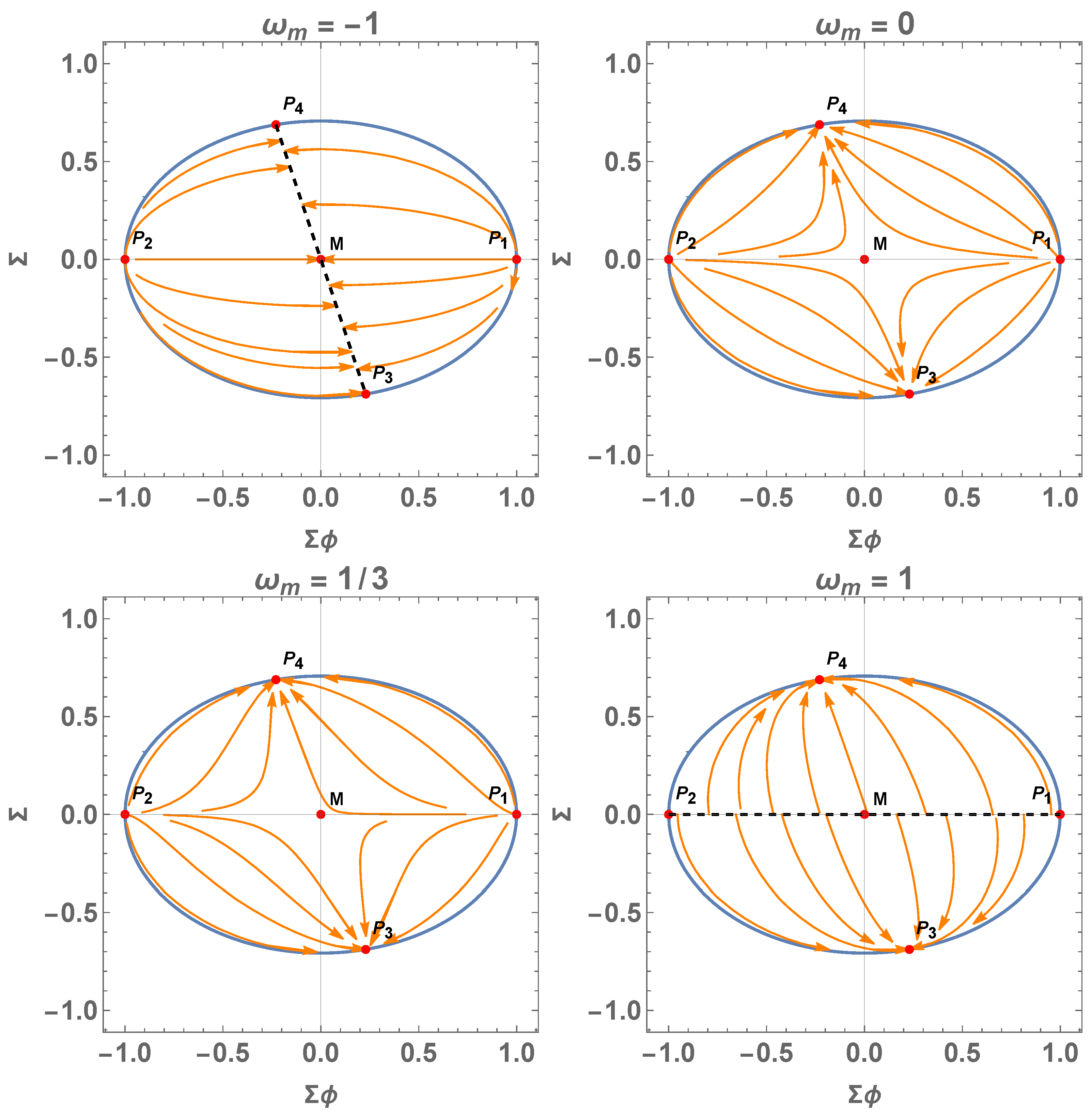
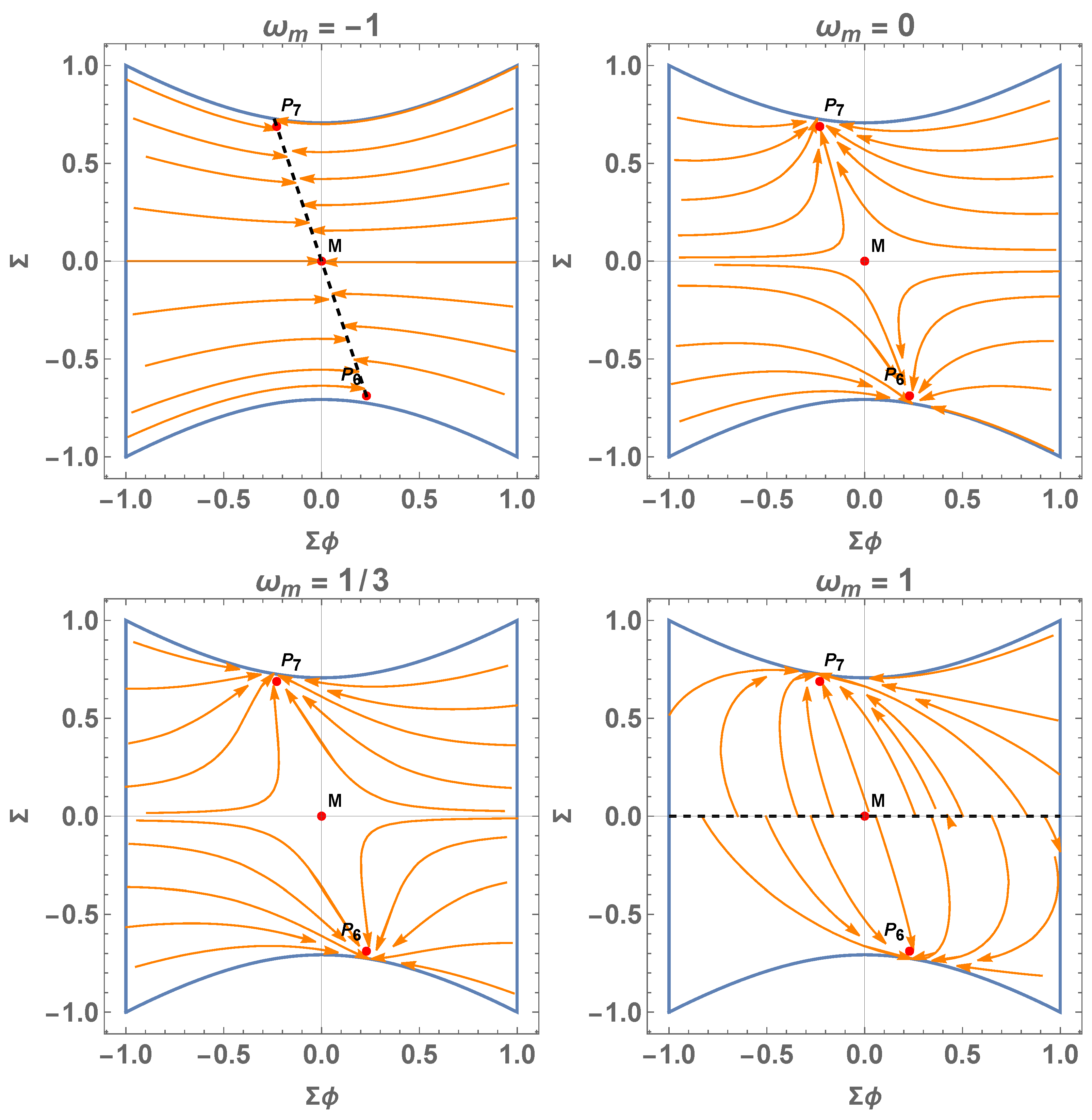
5.2. Reduced 2D System

Eliminate Ω m from (81) to obtain the reduced system:
Σ ϕ = 1 2 Σ ϕ 2 ϵ 1 ( 3 ( w m 1 ) Σ ϕ 2 Σ ) 3 2 μ ( w m + 1 ) Σ ϕ Σ 2 ,
Σ = 3 2 ( w m + 1 ) Σ 1 Σ ϕ 2 ϵ μ Σ 2 + Σ ϕ Σ ϵ ( 3 Σ ϕ + Σ ) .

5.2.1. Case ϵ = + 1

The equilibrium points of the system (85) and (86) are P 1 , 2   L 1 , P 3 , P 4 , and M, as summarized in Table 5.
Figure 7 presents the 2D projections of the system (85)–(86) for ϵ = + 1 , μ = 2 , and different values of ω m .

5.2.2. Case ϵ = 1

The equilibrium points of the system (85) and (86) for ϵ = 1 are summarized in Table 6.
Figure 8 presents the 2D projection of (85)–(86) for ϵ = 1 , μ = 2 , and different values of ω m .

6. Conclusions

In this study, we investigated the effects of the modification of the Poisson algebra on the dynamics of scalar field cosmology. Specifically, we performed a detailed phase space analysis by studying the equilibrium points and their stability, reconstructing the cosmological history.
The modified Poisson algebra modifies the field equations, introducing a cosmological constant term. The pressure component of the scalar field’s energy-momentum tensor is different from that of the canonical scalar field. Moreover, a mass term for the scalar field is introduced, which is described by the cosmological constant.
As a result, the equilibrium points provided by the modified field equations are different from those of the usual scalar field model. From the analysis, we can conclude that the modified equations can provide more than one accelerating universe, described by the de Sitter solution. Hence, cosmic inflation and late-time acceleration are provided by the specific theory.
In the matter-less case, we divided the study into two subcases, one for ϵ = 1 and one for ϵ = 1 . We have six families of physically acceptable equilibrium points that can describe stiff fluid solutions and de Sitter spacetime in the asymptotic regime.
In the case with the matter, we also considered the subcases ϵ = ± 1 , and in total, we obtained eight families of equilibrium points, the same ones as in the case without matter and one additional equilibrium point that describes matter.
In future work, we plan to further investigate the modified field equations with the introduction of a nonzero scalar field potential. In contrast, an interacting term between the scalar field and the matter source will be considered.
The steps in this paper allow exploring the cosmological models’ feasibility in concordance with the observational data set from measurements of Supernovae Ia, Cosmic Chronometers, baryon acoustic oscillation and cosmic microwave background. However, the observational test is out of the scope of the present research.

Author Contributions

G.L. managed the project, was involved in the asymptotic solutions, and wrote the final version of the paper. A.D.M. was involved in the asymptotic solutions, dynamical system analysis, and numerical integrations. A.P. organized the project, made the physical interpretation of the results and wrote the first draft. All authors have read and agreed to the published version of the manuscript.

Funding

Genly Leon was funded by Vicerrectoría de Investigación y Desarrollo Tecnológico (Vridt) at Universidad Católica del Norte (UCN) through Concurso De Pasantías De Investigación Año 2022, Resolución Vridt No. 040/2022, and through Resolución Vridt No. 054/2022. He also thanks the support of Núcleo de Investigación Geometría Diferencial y Aplicaciones, Resolución Vridt No. 096/2022. Andronikos Paliathanasis acknowledges Vridt-UCN through Concurso de Estadías de Investigación, Resolución VRIDT No. 098/2022. Alfredo David Millano was supported by Agencia Nacional de Investigación y Desarrollo (ANID) Subdirección de Capital Humano/Doctorado Nacional/año 2020 folio 21200837, Gastos operacionales proyecto de tesis/2022 folio 242220121, and Vridt-UCN.

Data Availability Statement

No new data were created or analyzed in this study. Data sharing is not applicable to this article.

Conflicts of Interest

The authors declare no conflict of interest.

References

  1. Tegmark, M.; Blanton, M.R.; Strauss, M.A.; Hoyle, F.; Schlegel, D.; Scoccimarro, R.; Vogeley, M.S.; Weinberg, D.H.; Zehavi, I.; Berlind, A.; et al. The 3-D power spectrum of galaxies from the SDSS. Astrophys. J. 2004, 606, 702. [Google Scholar] [CrossRef] [Green Version]
  2. Kowalsk, M.; Rubin, D.; Aldering, G.; Agostinho, R.J.; Amadon, A.; Amanullah, R.; Balland, C.; Barbary, K.; Blanc, G.; Challis, P.J.; et al. Improved Cosmological Constraints from New, Old, and Combined Supernova Data Sets. Astrophys. J. 2008, 686, 749. [Google Scholar] [CrossRef] [Green Version]
  3. Komatsu, E.; Dunkley, J.; Nolta, M.R.; Bennett, C.L.; Gold, B.; Hinshaw, G.; Jarosik, N.; Larson, D.; Limon, M.; Page, L.; et al. Five-Year Wilkinson Microwave Anisotropy Probe (WMAP) Observations: Cosmological Interpretation. Astrophys. J. Suppl. Ser. 2009, 180, 330. [Google Scholar] [CrossRef] [Green Version]
  4. Ade, P.A.R.; Aghanim, N.; Armitage-Caplan, C.; Arnaud, M.; Ashdown, M.; Atrio-Barandela, F.; Aumont, J.; Baccigalupi, C.; Banday, A.J.; Barreiro, R.B.; et al. Planck 2013 results. XV. CMB power spectra and likelihood. Astron. Astrophys. 2014, 571, A15. [Google Scholar]
  5. Padmanabhan, T. Cosmological constant—The weight of the vacuum. Phys. Rep. 2003, 380, 235. [Google Scholar] [CrossRef] [Green Version]
  6. Weinberg, S. The Cosmological Constant Problem. Rev. Mod. Phys. 1989, 61, 1. [Google Scholar] [CrossRef]
  7. Valentino, E.D.; Mena, O.; Pan, S.; Visinelli, L.; Yang, W.; Melchiorri, A.; Mota, D.F.; Reiss, A.G.; Silk, J. In the realm of the Hubble tension—A review of solutions. Class. Quantum Grav. 2021, 38, 153001. [Google Scholar]
  8. Ratra, B.; Peebles, P.J.E. Cosmological Consequences of a Rolling Homogeneous Scalar Field. Phys. Rev. D 1988, 37, 3406. [Google Scholar] [CrossRef]
  9. Chen, W.; Wu, Y.-.S. Implications of a cosmological constant varying as R**(-2). Phys. Rev. D 1990, 41, 695–698, Erratum in Phys. Rev. D 1992, 45, 4728. [Google Scholar] [CrossRef]
  10. Basilakos, S.; Plionis, M.; Solà, S. Hubble expansion & Structure Formation in Time Varying Vacuum Models. Phys. Rev. D 2009, 80, 3511. [Google Scholar]
  11. Wetterich, C. The Cosmon model for an asymptotically vanishing time dependent cosmological ‘constant’. Astron. Astrophys. 1995, 301, 321. [Google Scholar]
  12. Caldwell, R.R.; Dave, R.; Steinhardt, P.J. Cosmological imprint of an energy component with general equation of state. Phys. Rev. Lett. 1998, 80, 1582. [Google Scholar] [CrossRef] [Green Version]
  13. Brax, P.; Martin, J. Quintessence and supergravity. Phys. Lett. 1999, B468, 40. [Google Scholar] [CrossRef] [Green Version]
  14. Caldwell, R.R. A Phantom Menace? Cosmological consequences of a dark energy component with super-negative equation of state. Phys. Rev. Lett. B 2002, 545, 23. [Google Scholar] [CrossRef]
  15. Lima, J.A.S.; Silva, F.E.; Santos, R.C. Accelerating Cold Dark Matter Cosmology (ΩΛ≡0). Class. Quant. Grav. 2008, 25, 205006. [Google Scholar] [CrossRef] [Green Version]
  16. Brookfield, A.W.; van de Bruck, C.; Mota, D.F.; Tocchini-Valentini, D. Cosmology with massive neutrinos coupled to dark energy. Phys. Rev. Lett. 2006, 96, 061301. [Google Scholar] [CrossRef] [Green Version]
  17. Amendola, L.; Tsujikawa, S. Dark Energy Theory and Observations; Cambridge University Press: Cambridge, UK, 2010. [Google Scholar]
  18. Linde, A.D. Chaotic Inflation. Phys. Lett. B 1983, 129, 177. [Google Scholar] [CrossRef]
  19. Liddle, A.R. Power Law Inflation With Exponential Potentials. Phys. Lett. B 1989, 220, 502. [Google Scholar] [CrossRef]
  20. Charters, T.; Mimoso, J.P.; Nunes, A. Slow roll inflation without fine tuning. Phys. Lett. B 2000, 472, 21. [Google Scholar] [CrossRef] [Green Version]
  21. Barrow, J.D.; Saich, P. Scalar field cosmologies. Class. Quantum Grav. 1993, 10, 279. [Google Scholar] [CrossRef]
  22. Chervon, S.V.; Zhuravlev, V.M.; Shchigolev, V.K. New exact solutions in standard inflationary models. Phys. Lett. B 1997, 398, 269. [Google Scholar] [CrossRef] [Green Version]
  23. Kallosh, R.; Linde, A. Superconformal generalization of the chaotic inflation model λ4ϕ4-ξ2ϕ2R. JCAP 2013, 13, 027. [Google Scholar] [CrossRef] [Green Version]
  24. Paliathanasis, A. New inflationary exact solution from Lie symmetries. Mod. Phys. Lett. A 2022, 37, 2250119. [Google Scholar] [CrossRef]
  25. de Haro, J.; Amorós, J.; Pan, S. Simple inflationary quintessential model. Phys. Rev. D 2016, 93, 084018. [Google Scholar] [CrossRef]
  26. Starobinsky, A.A. A New Type of Isotropic Cosmological Models Without Singularity. Phys. Lett. B 1980, 91, 99. [Google Scholar] [CrossRef]
  27. Guth, A. The Inflationary Universe: A Possible Solution to the Horizon and Flatness Problems. Phys. Rev. D 1981, 23, 347. [Google Scholar] [CrossRef] [Green Version]
  28. Dolgov, A.D. An attempt to get rid of the Cosmological Constant. In The Very Early Universe; Gibbons, G., Hawking, S.W., Tiklos, S.T., Eds.; Cambridge University Press: Cambridge UK, 1982. [Google Scholar]
  29. Jassal, H.K.; Bagla, J.S.; Padmanabhan, T. Observational constraints on low redshift evolution of dark energy: How consistent are different observations? Phys. Rev. 2005, D72, 103503. [Google Scholar] [CrossRef] [Green Version]
  30. Jassal, H.K.; Bagla, J.S.; Padmanabhan, T. Understanding the origin of CMB constraints on dark energy. Mon. Not. R. Astron. Soc. Lett. 2005, 356, L11–L16. [Google Scholar] [CrossRef]
  31. Samushia, L.; Ratra, B. Cosmological Constraints from Hubble Parameter versus Redshift Data. Astrophys. J. 2006, 650, L5. [Google Scholar] [CrossRef] [Green Version]
  32. Samushia, L.; Ratra, B. Constraints on Dark Energy from Galaxy Cluster Gas Mass Fraction versus Redshift Data. Astrophys. J. 2008, 680, L1. [Google Scholar] [CrossRef] [Green Version]
  33. Simon, J.; Verde, L.; Jiménez, R. Constraints on the redshift dependence of the dark energy potential. Phys. Rev. 2005, D71, 123001. [Google Scholar] [CrossRef] [Green Version]
  34. Barrow, J.D.; Paliathanasis, A. Observational Constraints on New Exact Inflationary Scalar-field Solutions. Phys. Rev. D 2016, 94, 083518. [Google Scholar] [CrossRef] [Green Version]
  35. Pan, S.; Yang, W.; Paliathanasis, A. Imprints of an extended Chevallier–Polarski–Linder parametrization on the large scale of our universe. EPJC 2020, 80, 274. [Google Scholar] [CrossRef] [Green Version]
  36. Faraoni, V. Superquintessence. Int. J. Mod. Phys. D 2002, 11, 471. [Google Scholar] [CrossRef]
  37. Lima, J.A.S.; Alcaniz, J.S. Thermodynamics and spectral distribution of dark energy. Phys. Lett. B 2004, 600, 191. [Google Scholar] [CrossRef] [Green Version]
  38. Pereira, S.H.; Lima, J.A.S. On Phantom Thermodynamics. Phys. Lett. B 2008, 669, 266. [Google Scholar] [CrossRef] [Green Version]
  39. Paliathanasis, A.; Tsamparlis, M.; Basilakos, S. Dynamical symmetries and observational constraints in scalar field cosmology. Phys. Rev. D 2014, 90, 103524. [Google Scholar] [CrossRef] [Green Version]
  40. Martin, J.; Brandenberger, R.H. The TransPlanckian problem of inflationary cosmology. Phys. Rev. D 2001, 63, 123501. [Google Scholar] [CrossRef] [Green Version]
  41. Niemeyer, J.C. Inflation with a Planck scale frequency cutoff. Phys. Rev. D 2001, 63, 123502. [Google Scholar] [CrossRef]
  42. Kempf, A. Mode generating mechanism in inflation with cutoff. Phys. Rev. D 2001, 63, 083514. [Google Scholar] [CrossRef] [Green Version]
  43. Kempf, A.; Niemeyer, J. Perturbation spectrum in inflation with cutoff. Phys. Rev. D 2001, 64, 103501. [Google Scholar] [CrossRef] [Green Version]
  44. Ashoorioon, A.; Kempf, A.; Mann, R.B. Minimum length cutoff in inflation and uniqueness of the action. Phys. Rev. D 2005, 71, 023503. [Google Scholar] [CrossRef] [Green Version]
  45. Ashoorioon, A.; Hovdebo, J.L.; Mann, R.B. Running of the spectral index and violation of the consistency relation between tensor and scalar spectra from trans-Planckian physics. Nucl. Phys. B 2005, 727, 63–76. [Google Scholar] [CrossRef] [Green Version]
  46. Zampeli, A.; Paliathanasis, A. Quantization of inhomogeneous spacetimes with cosmological constant term. Class. Quantum Grav. 2021, 38, 165012. [Google Scholar] [CrossRef]
  47. Paliathanasis, A. Quantum potentiality in Inhomogeneous Cosmology. Universe 2021, 7, 52. [Google Scholar] [CrossRef]
  48. Zampeli, A.; Pailas, T.; Terzis, P.A.; Christodoulakis, T. Conditional symmetries in axisymmetric quantum cosmologies with scalar fields and the fate of the classical singularities. JCAP 2016, 05, 066. [Google Scholar] [CrossRef] [Green Version]
  49. Mukhi, S. String theory: A perspective over the last 25 years. Class. Quant. Grav. 2011, 28, 153001. [Google Scholar] [CrossRef] [Green Version]
  50. Kowalski-Glikman, J. Introduction to doubly special relativity. Lect. Notes Phys. 2005, 669, 131–159. [Google Scholar]
  51. Amelino-Camelia, G. Doubly-Special Relativity: Facts, Myths and Some Key Open Issues. Symmetry 2010, 2, 230–271. [Google Scholar] [CrossRef] [Green Version]
  52. Bekenstein, J.D. Black holes and entropy. Phys. Rev. D 1973, 7, 2333. [Google Scholar] [CrossRef]
  53. Bekenstein, J.D. Black Holes and the Second Law. Lett. Nuovo C 1972, 4, 737–740. [Google Scholar] [CrossRef]
  54. Maggiore, M. A Generalized uncertainty principle in quantum gravity. Phys. Lett. B 1993, 304, 65. [Google Scholar] [CrossRef] [Green Version]
  55. Giacomini, A.; Leon, G.; Paliathanasis, A.; Pan, S. Dynamics of Quintessence in Generalized Uncertainty Principle. Eur. Phys. J. C 2020, 80, 931. [Google Scholar] [CrossRef]
  56. Paliathanasis, A.; Leon, G.; Khyllep, W.; Dutta, J.; Pan, S. Interacting quintessence in light of generalized uncertainty principle: Cosmological perturbations and dynamics. Eur. Phys. J. C 2021, 81, 607. [Google Scholar] [CrossRef]
  57. Masood, S.; Faizal, M.; Zal, Z.; Ali, A.F.; Raza, J.; Shah, M.B. The most general form of deformation of the Heisenberg algebra from the generalized uncertainty principle. Phys. Lett. B 2016, 763, 218. [Google Scholar] [CrossRef]
  58. Rasouli, S.M.M.; Ziaie, A.H.; Marto, J.; Moniz, P.V. Gravitational Collapse of a Homogeneous Scalar Field in Deformed Phase Space. Phys. Rev. D 2014, 89, 044028. [Google Scholar] [CrossRef] [Green Version]
  59. Jalalzadeh, S.; Rasouli, S.M.M.; Moniz, P.V. Quantum cosmology, minimal length and holography. Phys. Rev. D 2014, 90, 023541. [Google Scholar] [CrossRef] [Green Version]
  60. Rasouli, S.M.M.; Farhoudi, M.; Vargas Moniz, P. Modified Brans–Dicke theory in arbitrary dimensions. Class. Quant. Grav. 2014, 31, 115002. [Google Scholar] [CrossRef] [Green Version]
  61. Rasouli, S.M.M.; Vargas Moniz, P. Noncommutative minisuperspace, gravity-driven acceleration, and kinetic inflation. Phys. Rev. D 2014, 90, 083533. [Google Scholar] [CrossRef] [Green Version]
  62. Rasouli, S.M.M.; Ziaie, A.H.; Jalalzadeh, S.; Moniz, P.V. Non-singular Brans–Dicke collapse in deformed phase space. Ann. Phys. 2016, 375, 154–178. [Google Scholar] [CrossRef] [Green Version]
  63. Rasouli, S.M.M.; Vargas Moniz, P. Gravity-Driven Acceleration and Kinetic Inflation in Noncommutative Brans-Dicke Setting. Odessa Astron. Pub. 2016, 29, 19. [Google Scholar] [CrossRef] [Green Version]
  64. Jalalzadeh, S.; Capistrano, A.J.S.; Moniz, P.V. Quantum deformation of quantum cosmology: A framework to discuss the cosmological constant problem. Phys. Dark Univ. 2017, 18, 55–66. [Google Scholar] [CrossRef] [Green Version]
  65. Pérez-Payán, S.; Sabido, M.; Yee-Romero, C. Effects of deformed phase space on scalar field cosmology. Phys. Rev. D 2013, 88, 027503. [Google Scholar] [CrossRef] [Green Version]
  66. Tajahmad, B. Late-time-accelerated expansion esteemed from minisuperspace deformation. Eur. Phys. J. C 2022, 82, 965. [Google Scholar] [CrossRef]
  67. Tavakol, R. Introduction to Dynamical Systems; Cambridge University Press: Cambridge, UK, 1997; pp. 84–104. [Google Scholar]
  68. Copeland, E.J.; Liddle, A.R.; Wands, D. Exponential potentials and cosmological scaling solutions. Phys. Rev. D 1998, 57, 4686–4690. [Google Scholar] [CrossRef]
  69. Coley, A.A. Dynamical Systems and Cosmology; Kluwer: Dordrecht, The Netherlands, 2003. [Google Scholar]
  70. Leon, G.; Fadragas, C.R. Cosmological Dynamical Systems; LAP LAMBERT Academic Publishing: Saarbrücken, Germany, 2012; ISBN 978-3-8473-0233-9. [Google Scholar]
  71. Gong, Y.; Wang, A.; Zhang, Y.-Z. Exact scaling solutions and fixed points for general scalar field. Phys. Lett. B 2006, 636, 286–292. [Google Scholar] [CrossRef] [Green Version]
  72. Setare, M.R.; Saridakis, E.N. Quintom dark energy models with nearly flat potentials. Phys. Rev. D 2009, 79, 043005. [Google Scholar] [CrossRef] [Green Version]
  73. Chen, X.M.; Gong, Y.-G. Saridakis, E.N. Phase-space analysis of interacting phantom cosmology. JCAP 2009, 04, 001. [Google Scholar]
  74. Gupta, G.; Saridakis, E.N.; Sen, A.A. Non-minimal quintessence and phantom with nearly flat potentials. Phys. Rev. D 2009, 79, 123013. [Google Scholar] [CrossRef]
  75. Farajollahi, H.; Salehi, A.; Tayebi, F.; Ravanpak, A. Stability Analysis in Tachyonic Potential Chameleon cosmology. JCAP 2011, 05, 017. [Google Scholar] [CrossRef]
  76. Arturo Urena-Lopez, L. Unified description of the dynamics of quintessential scalar fields. JCAP 2012, 03, 035. [Google Scholar] [CrossRef] [Green Version]
  77. Escobar, D.; Fadragas, C.R.; Leon, G.; Leyva, Y. Phase space analysis of quintessence fields trapped in a Randall-Sundrum Braneworld: A refined study. Class. Quant. Grav. 2012, 29, 175005. [Google Scholar] [CrossRef] [Green Version]
  78. Escobar, D.; Fadragas, C.R.; Leon, G.; Leyva, Y. Phase space analysis of quintessence fields trapped in a Randall-Sundrum Braneworld: Anisotropic Bianchi I brane with a Positive Dark Radiation term. Class. Quant. Grav. 2012, 29, 175006. [Google Scholar] [CrossRef] [Green Version]
  79. Xu, C.; Saridakis, E.N.; Leon, G. Phase-Space analysis of Teleparallel Dark Energy. JCAP 2012, 07, 005. [Google Scholar] [CrossRef]
  80. Leon, G.; Saavedra, J.; Saridakis, E.N. Cosmological behavior in extended nonlinear massive gravity. Class. Quant. Grav. 2013, 30, 135001. [Google Scholar] [CrossRef] [Green Version]
  81. Burd, A.B.; Barrow, J.D. Inflationary Models with Exponential Potentials. Nucl. Phys. B 1988, 308, 929–945, Erratum in Nucl.Phys. B 1989, 324, 276. [Google Scholar] [CrossRef]
  82. de Vegvar, P.G.N. Commutatively deformed general relativity: Foundations, cosmology, and experimental tests. Eur. Phys. J. C 2021, 81, 786. [Google Scholar] [CrossRef]
  83. Basilakos, S.; Tsamparlis, M.; Paliathanasis, A. Using the Noether symmetry approach to probe the nature of dark energy. Phys. Rev. D 2011, 83, 103512. [Google Scholar] [CrossRef] [Green Version]
  84. Paliathanasis, A.; Tsamparlis, M. Two scalar field cosmology: Conservation laws and exact solutions. Phys. Rev. D 2014, 90, 043529. [Google Scholar] [CrossRef] [Green Version]
  85. Paliathanasis, A.; Leon, G.; Pan, S. Exact Solutions in Chiral Cosmology. Gen. Rel. Grav. 2019, 51, 106. [Google Scholar] [CrossRef]
Figure 1. Phase plot for System (68)–(69) for ϵ = + 1 and different values of μ . The dashed black line corresponds to L 1 .
Mathematics 11 00120 g001
Figure 2. Phase plot for System (68)–(69) for ϵ = 1 and different values of μ . The dashed black line corresponds to L 1 .
Mathematics 11 00120 g002
Figure 3. Phase plot for the reduced 1D equation (77) for ϵ = ± 1 and μ = 2 .
Mathematics 11 00120 g003
Figure 4. Phase plot for the reduced 1D equation (79) for ϵ = ± 1 and μ = 2 .
Mathematics 11 00120 g004
Figure 5. The 3D phase plot for System (82), (83), and (84) for ϵ = + 1 , μ = 2 , and different values of ω m .
Mathematics 11 00120 g005
Figure 6. The 3D phase plot for System (82), (83), and (84) for ϵ = 1 , μ = 2 , and different values of ω m .
Mathematics 11 00120 g006
Figure 7. The 2D projections of the system (85)–(86) for ϵ = + 1 , μ = 2 , and different values of ω m .
Mathematics 11 00120 g007
Figure 8. The 2D projection of (85)–(86) for ϵ = 1 , μ = 2 , and different values of ω m .
Mathematics 11 00120 g008
Table 1. Equilibrium points of System (68)–(69) for ϵ = + 1 with their eigenvalues and stability. P 5 is a sink, but does not satisfy the condition (65).
LabelExistenceCoordinates ( Σ ϕ , Σ ) EigenvaluesStability
P 1 , 2 ϵ = + 1 ( ± 1 , 0 ) { 3 , 6 } Unstable
L 1 always ( Σ ϕ , 3 Σ ϕ ) { 3 , 0 } Stable
P 3 , 6 ϵ = ± 1 ϵ 9 μ + ϵ , 3 ϵ 9 μ + ϵ { 3 , 0 } Stable
P 4 , 7 ϵ = ± 1 ϵ 9 μ + ϵ , 3 ϵ 9 μ + ϵ { 3 , 0 } Stable
P 5 ( 0 , 0 ) { 3 , 0 } Stable
Table 2. Equilibrium points of System (77) for ϵ = ± 1 with their eigenvalues and stability.
LabelExistenceCoordinates Σ ϕ EigenvalueStability
P 1 , 2 ϵ = + 1 ± 1 6Unstable
P 3 ϵ = + 1 , μ > 1 9 1 9 μ + 1 3 Stable
P 6 ϵ = 1 , μ > 1 9 1 9 μ 1 3 Stable
Table 3. Equilibrium points of System (79) for ϵ = ± 1 with their eigenvalues and stability.
LabelExistenceCoordinates Σ ϕ EigenvalueStability
P 1 , 2 ± 1 ϵ = + 1 6Unstable
P 4 ϵ = + 1 , μ > 1 9 1 9 μ + 1 3 Stable
P 7 ϵ = 1 , μ > 1 9 1 9 μ 1 3 Stable
Table 4. Equilibrium points of System (82), (83), and (84) for ϵ = ± 1 with their eigenvalues and stability.
LabelExistenceCoordinates ( Σ ϕ , Σ , Ω m ) EigenvaluesStability
P 1 , 2 ϵ = + 1 ( ± 1 , 0 , 0 ) { 3 , 6 , 3 ( 1 ω m ) } Unstable
L 1 always ( Σ ϕ , 3 Σ ϕ , 0 ) { 3 , 0 , 3 ( ω m + 1 ) } Stable
P 3 , 6 ϵ = ± 1 ϵ 9 μ + ϵ , 3 ϵ 9 μ + ϵ , 0 { 3 , 0 , 3 ( ω m + 1 ) } Stable
P 4 , 7 ϵ = ± 1 ϵ 9 μ + ϵ , 3 ϵ 9 μ + ϵ , 0 { 3 , 0 , 3 ( ω m + 1 ) } Stable
P 5 ( 0 , 0 , 0 ) { 3 , 0 , 3 ( ω m + 1 ) } Stable
M ϵ = ± 1 ( 0 , 0 , 1 ) 3 ( ω m 1 ) 2 , 3 ( ω m + 1 ) 2 , 3 ( ω m + 1 ) Stable for ω m = 1
Unstable for ω m = 1
Saddle otherwise
Table 5. Equilibrium points of System (85) and (86) for ϵ = + 1 with their eigenvalues and stability.
LabelCoordinates ( Σ ϕ , Σ ) EigenvaluesStability
P 1 , 2 ( ± 1 , 0 ) { 3 , 6 } Unstable
L 1 ( Σ ϕ , 3 Σ ϕ ) { 3 , 3 ( ω + 1 ) } Stable
P 3 1 9 μ + 1 , 3 9 μ + 1 { 3 , 3 ( ω + 1 ) } Stable
P 4 1 9 μ + 1 , 3 9 μ + 1 { 3 , 3 ( ω + 1 ) } Stable
M ( 0 , 0 ) 3 ( ω m 1 ) 2 , 3 ( ω m + 1 ) Stable for ω = 1
Unstable for ω = 1
Saddle otherwise
Table 6. Equilibrium points of System (85) and (86) for ϵ = 1 with their eigenvalues and stability.
LabelCoordinates ( Σ ϕ , Σ ) EigenvaluesStability
L 1 ( Σ ϕ , 3 Σ ϕ ) { 3 , 3 ( ω m + 1 ) } Stable
P 6 1 9 μ 1 , 3 9 μ 1 { 3 , 3 ( ω + 1 ) } Stable
P 7 1 9 μ 1 , 3 9 μ 1 { 3 , 3 ( ω + 1 ) } Stable
M ( 0 , 0 ) 3 ( ω m 1 ) 2 , 3 ( ω m + 1 ) Stable for ω = 1
Unstable for ω = 1
Saddle otherwise
Disclaimer/Publisher’s Note: The statements, opinions and data contained in all publications are solely those of the individual author(s) and contributor(s) and not of MDPI and/or the editor(s). MDPI and/or the editor(s) disclaim responsibility for any injury to people or property resulting from any ideas, methods, instructions or products referred to in the content.

