Article

Chenciner Bifurcation Presenting a Further Degree of Degeneration

by
Sorin Lugojan
1,†,
Loredana Ciurdariu
1,*,† and
Eugenia Grecu
2,†
1
Department of Mathematics, Politehnica University of Timisoara, 300006 Timisoara, Romania
2
Department of Management, Politehnica University of Timisoara, 300006 Timisoara, Romania
*
Author to whom correspondence should be addressed.
These authors contributed equally to this work.
Mathematics 2022, 10(9), 1603; https://doi.org/10.3390/math10091603
Submission received: 19 March 2022 / Revised: 30 April 2022 / Accepted: 5 May 2022 / Published: 8 May 2022
(This article belongs to the Special Issue Dynamical System and Stochastic Analysis)

Abstract

:
Chenciner bifurcation appears for some two-dimensional systems with discrete time having two independent variables. Investigated here is a special case of degeneration where the implicit function theorem cannot be used around the origin, so a new approach is necessary. In this scenario, there are many more bifurcation diagrams than in the two non-degenerated cases. Several numerical simulations are presented.
MSC:
37L10; 37G10

1. Introduction

The discrete dynamical systems have an increasing role in informatics [1], computer and machine learning, and other interdisciplinary fields [2,3,4]. A new mathematical model was recently proposed in [5] for the dynamics of three types of phytoplankton of the Sea of Azov under the condition of salinity increase. Other examples of applied dynamical discrete systems, besides continuous ones, are given in [6,7,8,9]. Presented among them is a discrete-time epidemic model applied to the study of the COVID-19 virus [8]. The theory of discrete dynamical systems may be applied in many branches of engineering such as suspension bridges, ball bearings, and nanotechnology. The study of impact oscillators is an important source of nonlinearity in mechanical system theory [10,11,12,13]. When the impact has zero velocity, the so-called grazing impacts appear. The near-grazing systems can be described by discrete dynamical systems, and an application for harmonic oscillators is presented in [12]. The dynamics of the other two types of discrete dynamical systems, a discrete predator-prey model with group defense and nonlinear harvesting in prey and a modified Nicholson-Bailey model, were investigated, and the conditions for classical Neimark-Sacker bifurcation were given in [14,15].
Economy is another important domain of application [16]. Traditionally, economic agents are considered to have rational expectations [17], which assume that prices follow the fundamental economic value. Experiments have shown that economic agents [18] do not make rational predictions but follow empirical rules. Thus, sometimes these rules can lead them to the fundamental landmark, but other times they can be coordinated on destabilizing strategies to follow the trends. The consequences are market “bubbles” and even collapses. A “bubble” represents a strong over evaluation [19] and the duration of an asset compared to its fundamental economic value. Big “bubbles” and sudden market crashes are difficult to harmonize with the standard model of agents representing rational expectations. Some authors, for example [20], have devised a simple behavioral heuristic switching model that explains the path-dependent coordination of the individual forecast, as well as the aggregate behavior of the market. The paper analyzes the coexistence of a locally stable fundamental equilibrium state and a stable quasi-periodic orbit, created by the Chenciner bifurcation. In relation to the initial states, the economic agents will orient their individual expectations either on a stable fundamental equilibrium trajectory or on persistent price fluctuations in the vicinity of the fundamental equilibrium state.
The generalized Neimark-Sacker bifurcations or Chenciner bifurcations of discrete dynamical systems have been discovered in 1985 in [21,22,23], in the framework of the study of elliptic bifurcations of fixed points. Later, in 1990 in [24] this bifurcation was characterized better than before. The non-degenerate Chenciner bifurcation is one of the eleven types retrieved in the generic two-parameter discrete-time dynamical systems, according to classification from [25]. There is no other bifurcation of codimension 2 in generic discrete-time systems. The non-degeneracy condition, so called “cubic non-degeneracy”, is not fulfilled in this case of the generalized Neimark-Sacker bifurcations.
In recent years, the study of degenerated discrete Chenciner bifurcation began, as seen in [26]. The singularities are always difficult to study in comparison to the regular cases. The purpose of this article is to examine the Chenciner bifurcation which doesn’t check the condition (CH.1) [25] (p. 405). That is the degenerated Chenciner bifurcation. The two types of bifurcation diagrams existing in the non-degenerated variant, as seen in [25], are replaced by 32 types of bifurcation diagrams in a particular degenerated discrete Chenciner dynamical system; see [26].
The article is composed of four sections. The first section is the Introduction, where the non-degenerate Chenciner bifurcations are presented using the truncated normal form of the system (A4) and polar coordinates, and some new applications in various domains are mentioned. Section two of this paper describes the results given in [26,27] concerning the existence of bifurcation curves and their dynamics in the parametric plane ( α 1 , α 2 ) in the cases where a 10 b 01 a 01 b 10 0 and the linear parts of β 1 α and β 2 α nullify, respectively, and when a 10 = 0 , b 01 = 0 , a 01 = 0 and b 10 = 0 . The third section is the main part of the paper, where the degeneracy case of the Chenciner bifurcation written in the truncated normal form was studied when a 20 = a 11 = a 02 = 0 and, for b 10 and b 01 , two situations have been studied: b 10 0 , b 01 0 or b 10 = b 01 = 0 . In addition, some numerical simulations are presented using Matlab for checking the theoretical results. The discussions and conclusions are presented in the fourth section of the paper.

2. Methods

The study of the non-degenerated discrete Chenciner bifurcation begins by a defect of a coordinate change ( α 1 , α 2 ) ( β 1 , β 2 ) . The degeneration taken into account is a non-regularity of the coordinate change in the origin, which loses its quality of coordinate change. The method introduced [26] is to consider the same expression for β 1 , β 2 but as functions of α 1 , α 2 and not as new coordinates.
The steps of the method used in previous papers for finding the truncated normal form of generalized Neimark-Sacker bifurcation for analyzing the behavior of such general two-dimensional discrete dynamical systems in order to obtain the bifurcation diagrams are given in Appendix A. The Chenciner bifurcations imply that the center manifold for the Poincare map is two-dimensional. In [26], a new degeneration for generalized Neimark-Sacher bifurcations was introduced; therefore, the classical Chenciner bifurcations are called non-degenerate Chenciner bifurcations. This study has been continued in [27,28] and also in the present paper. In the degenerated case, there are two different approaches: the first is to work with the initial parameters α 1 , α 2 in the polar form, (A6) of our system, and the second, in [28], is considered another regular transformation of parameters, when the product a 10 a 01 b 10 b 01 0 .
The following two results, Theorems A1 and A2, which have been established in [26], play a key role in the next section and will be restated in Appendix B. Theorem A1 establishes the stability of the fix point O function of the sign of β 1 ( α ) , and then, in Theorem A2, the existence of invariant circles is discussed as a function of the sign of Δ ( α ) . From here, the generic phase portraits corresponding to different regions of the bifurcation diagrams were obtained in Figure 1 from [26] and in Appendix B, Figure A1. Table 1 from [26] gives the regions in the parametric plane defined by Δ ( α ) , β 1 ( α ) , β 2 ( α ) , and L 0 . These phase portraits remain the same, but the bifurcation diagrams are different from the non-degenerate Chenciner bifurcation case in [25]. These kinds of studies represent important topics in the qualitative theory of discrete-time dynamical systems.
Now, we will write the smooth functions β 1 , 2 α as β 1 α = a 10 α 1 + a 01 α 2 + i + j 2 a i j α 1 i α 2 j and β 2 α = b 10 α 1 + b 01 α 2 + i + j 2 b i j α 1 i α 2 j for our further goals. We recall that the transformation (A7) is not regular at 0 , 0 . That means the Chenciner bifurcation becomes degenerate, iff
a 10 b 01 a 01 b 10 = 0 .
The case when the linear part of β 1 α nullifies and β 2 α has at least one linear term was mentioned in [27] together with Theorem 2 of [27], which is an important result concerning the existence, and also the relative positions in the parametric plane, ( α 1 , α 2 ) of the bifurcation curves, function of the sign of β 1 ( α ) .
Recently, in [27], the dynamics of the system in the form (A10) and (A11) was described and studied in the case when all these coefficients a 10 = 0 , b 01 = 0 , a 01 = 0 and b 10 = 0 , and the bifurcation diagrams obtained are different from previous situations form [26,28].
In this paper, the degeneracy condition (1) will be satisfied and the terms of degree one and two are zero in the case of β 1 ( α ) . Therefore, the functions β 1 , 2 α become
β 1 α = a α 2 3 + b α 1 α 2 2 + c α 1 2 α 2 + d α 1 3 + i + j = 4 p 1 a i j α 1 i α 2 j + O α p 1 + 1
and
β 2 α = k α 1 + h α 2 + i + j = 2 q 1 b i j α 1 i α 2 j + O α q 1 + 1
for some p 1 4 . a = a 03 , b = a 12 , c = a 21 , d = a 30 , respectively, and q 1 2 , h = b 10 , k = b 01 .
The set B 1 , 2 and C will be denoted by
B 1 , 2 = α 1 , α 2 R 2 , β 1 , 2 α = 0 , α < ε
and
C = α 1 , α 2 R 2 , Δ α = 0 , α < ε
for some ε > 0 that is sufficiently small, and then the new Δ ( α ) is
Δ α = β 2 2 α 4 β 1 α L 2 α .

3. Results

In this section, the degree of the truncated version of the first bifurcation curve, β 1 , is D e g β 1 = 3 , and for the second bifurcation curve, β 2 , two cases will be studied: when the D e g β 2 = 1 and when the D e g β 2 = 2 in the truncated version.

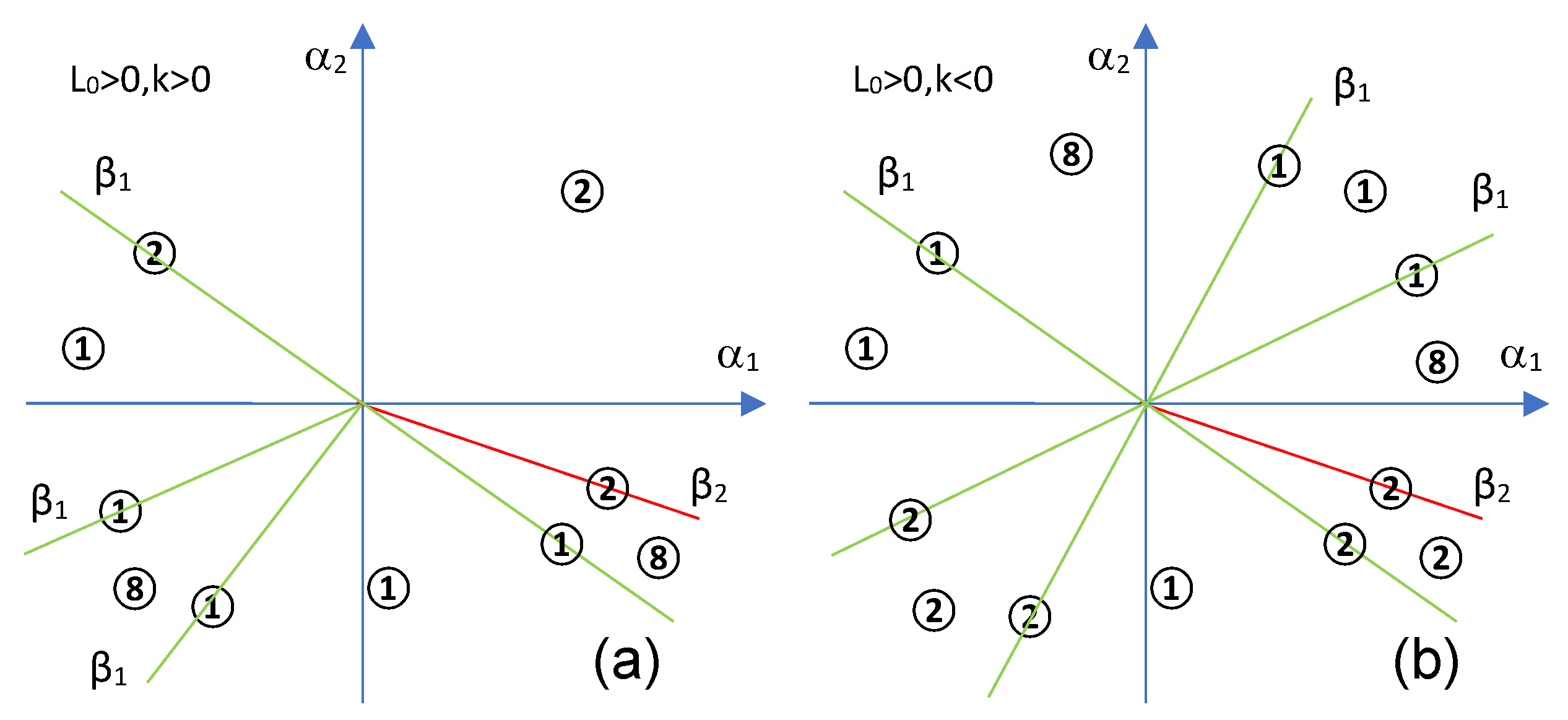
3.1. Degree of the Second Bifurcation Curve Is One in the Truncated Version

Firstly, we focus on the case when Deg β 2 = 1 in the truncated version. In expression of β 1 ( α ) , we denote the coefficients a 03 , a 12 , a 21 , and a 30 by a, b, c, and d, respectively, and in expression of β 2 ( α ) , we denote the coefficients b 01 and b 10 by h and k, respectively.
β 1 ( α 1 , α 2 ) = a α 2 3 + b α 2 2 α 1 + c α 2 α 1 2 + d α 1 3 + O ( | α | 4 ) ,
where a , b , c , d R * .
β 2 ( α 1 , α 2 ) = h α 2 + k α 1 + O ( | α | 2 ) ,
where h , k R * .
Then
Δ ( α ) = [ β 2 ( α ) ] 2 4 L 2 ( α ) β 1 ( α ) ,
where α = ( α 1 , α 2 ) .
In the truncated version, we have:
β 1 ( α ) = a α 2 3 + b α 2 2 α 1 + c α 2 α 1 2 + d α 1 3
β 2 ( α ) = h α 2 + k α 1
Δ ( α ) = [ β 2 ( α ) ] 2
Discussed below is the sign of first bifurcation curve in the truncated version.
In order to establish the sign of β 1 ( α ) , the following is used:
Remark 1.
The sign of the polynomial
β 1 ( T ) = a T 3 + b T 2 + c T + d R * [ T ] ,
is the same as the sign of β 1 ( α 1 , α 2 ) , for every α 1 , α 2 R , such that α 2 = T α 1 .
In order to establish the sign of β 1 ( T ) , we denote, as usual for the third degree equation:
p = c a b 2 3 a 2 , q = 2 b 3 27 a 3 b c 3 a 2 + d a ,
and the polynomial becomes:
β 1 ( T ) = a ( T 3 + p T + q ) .
The roots of β 1 ( T ) are the solutions of the equation
T 3 + p T + q = 0 .
For the classification of the β 1 ( T ) roots, we use the notation
r = q 2 2 + p 3 3
which is called “the cubic discriminant”.
  • For p > 0 , q 0 , there is one real root e 1 , and two complex conjugated ones;
  • For p < 0 , q = 0 , there is a triple root e 1 ;
  • For p < 0 , r > 0 , there is one real root e 1 , and two complex conjugated ones;
  • For p < 0 , r = 0 , there are three real roots, one simple e 1 , and two common;
  • For p < 0 , r < 0 , there are three real different roots e 1 < e 2 < e 3 .
Lemma 1.
The following statements are true:
  • If p < 0 and r < 0 , then
    s i g n [ β 1 ( T ) ] = s i g n [ a ( T e 1 ) ( T e 2 ) ( T e 3 ) ] ,
    see Table 1.
  • If p > 0 or ( p < 0 and r 0 ), then
    s i g n [ β 1 ( T ) ] = s i g n [ a ( T e 1 ) ] ,
    see Table 2.
The case when p and r are strictly negative are rendered below.
From Appendix A, θ 0 = θ ( 0 ) and L 0 = L 2 ( 0 ) 0 . The case p < 0 , r < 0 involves four cases to analyze, impossing that h k > 0 .
  • L 0 > 0 , k > 0
  • L 0 > 0 , k < 0
  • L 0 < 0 , k > 0
  • L 0 < 0 , k < 0 .
The bifurcation diagrams are respectively given in Figure 1, Figure 2, Figure 3 and Figure 4.
Remark 2.
When β 2 ( α ) = 0 , then the sign of Δ ( α ) is given by the relation (7), instead of (8).
The case when p is strictly positive or (p is strictly negative and r is positive) will be studied below.
In the case p > 0 or ( p < 0 and r 0 ), from Lemma 1 (2), it results that s i g n [ β 1 ( T ) ] = s i g n [ a ( T e 1 ) ] , see Table 2, where e 1 is the unique real root of β 1 ( α ) = 0 . From β 2 ( α ) = h α 2 + k α 1 , it results that m 2 = k h . In our case, Δ ( α ) = [ β 2 ( α ) ] 2 . We impose that h k > 0 .
Therefore we will have the following two bifurcation diagrams presented in Figure 3.
Remark 3.
In the case p > 0 or ( p < 0 and r 0 ), we will obtain only two distinct figures; that means the following Figure 3a,b:
  • if a > 0 , k > 0 , L 0 > 0 or a > 0 , k < 0 , L 0 > 0 or a < 0 , k > 0 , L 0 > 0 or a < 0 , k < 0 , L 0 > 0 , we get Figure 3a;
  • if a > 0 , k > 0 , L 0 < 0 or a > 0 , k < 0 , L 0 < 0 or a < 0 , k > 0 , L 0 < 0 or a < 0 , k < 0 , L 0 < 0 , we get Figure 3b.

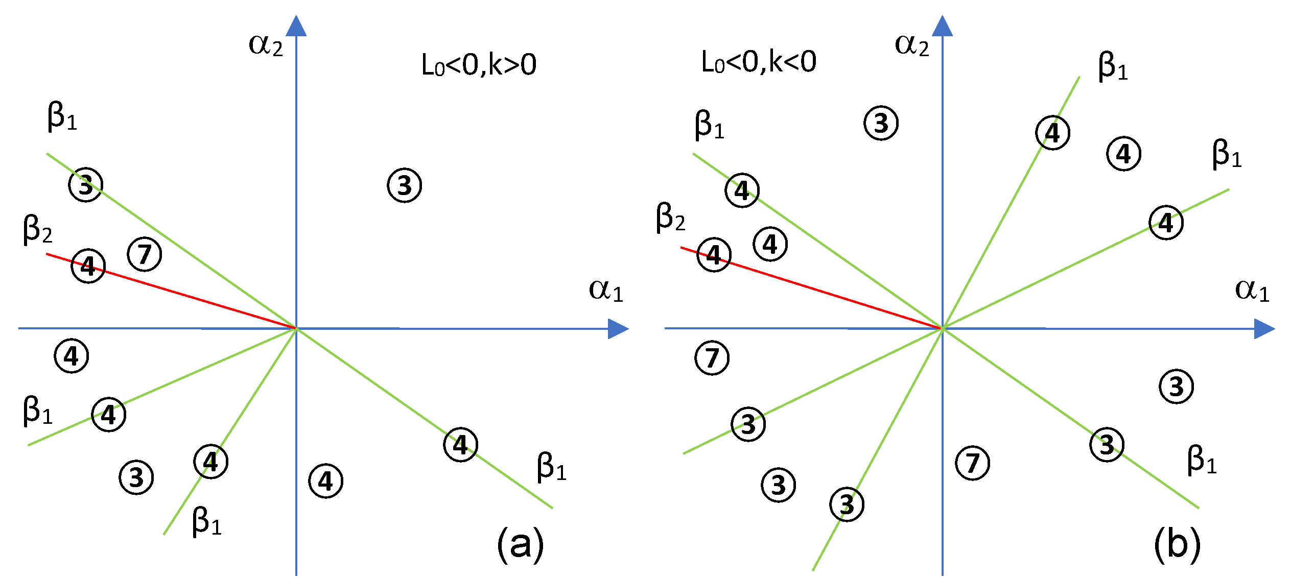
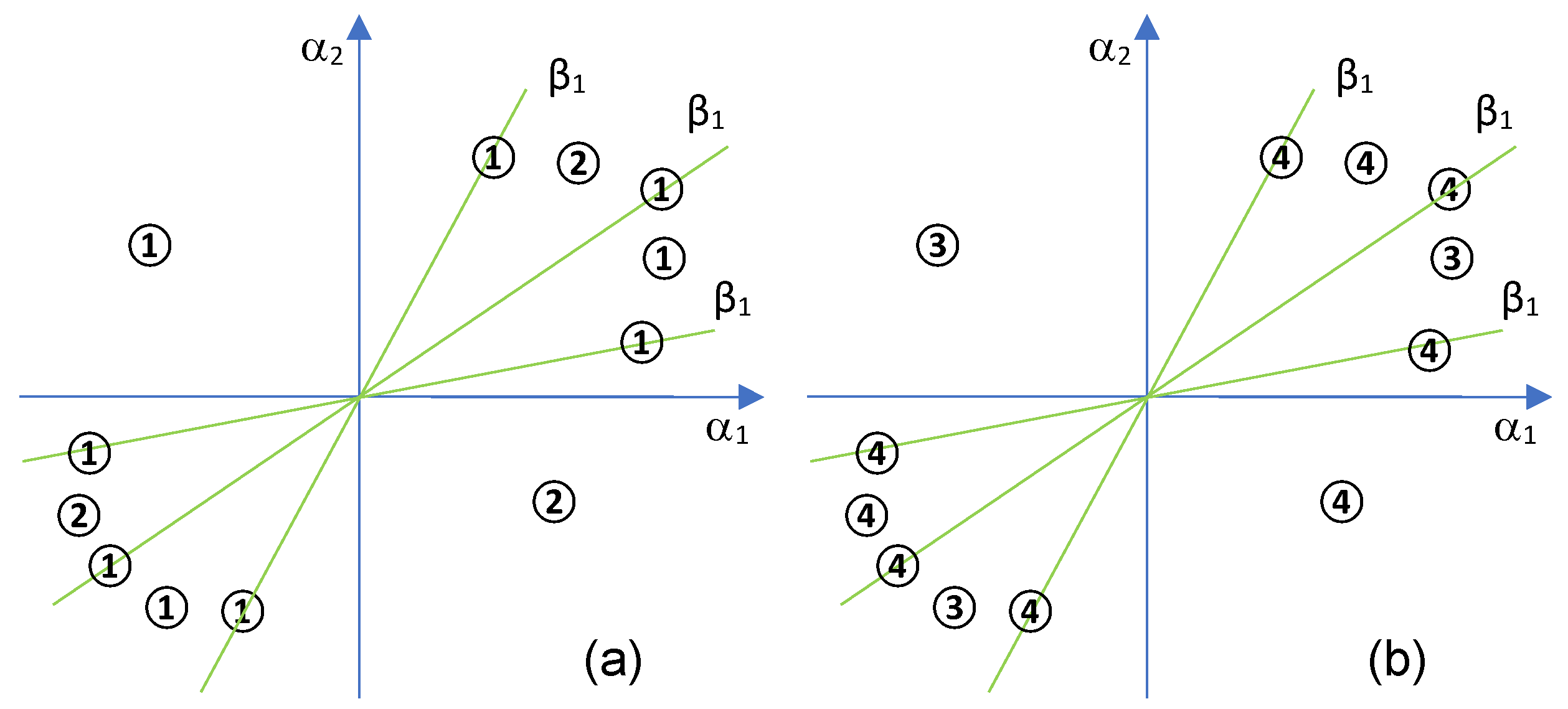
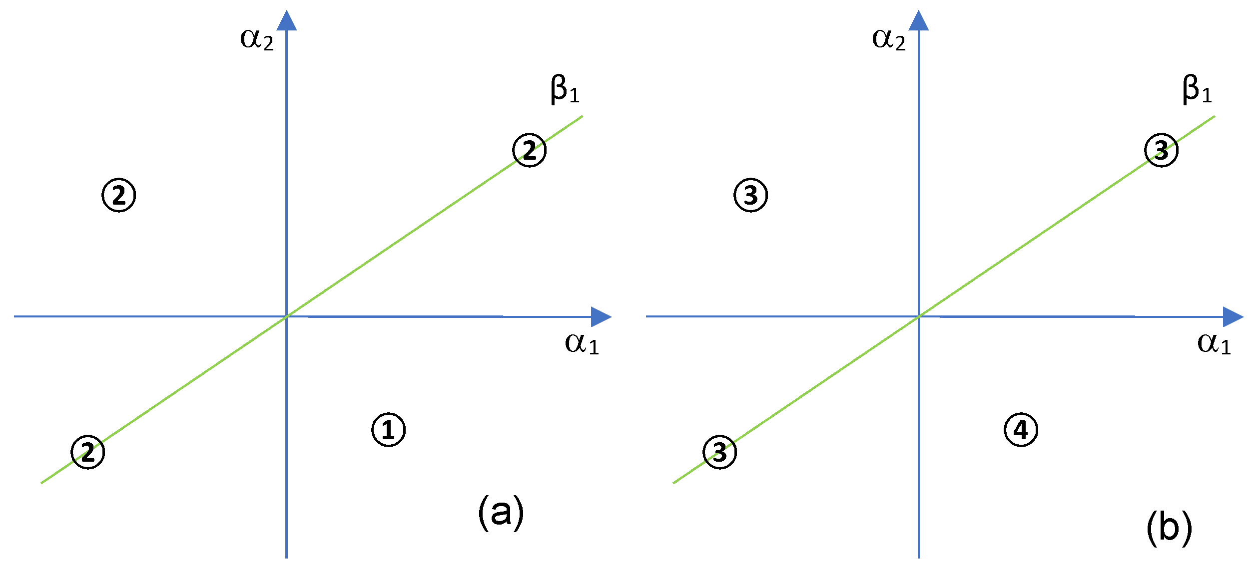
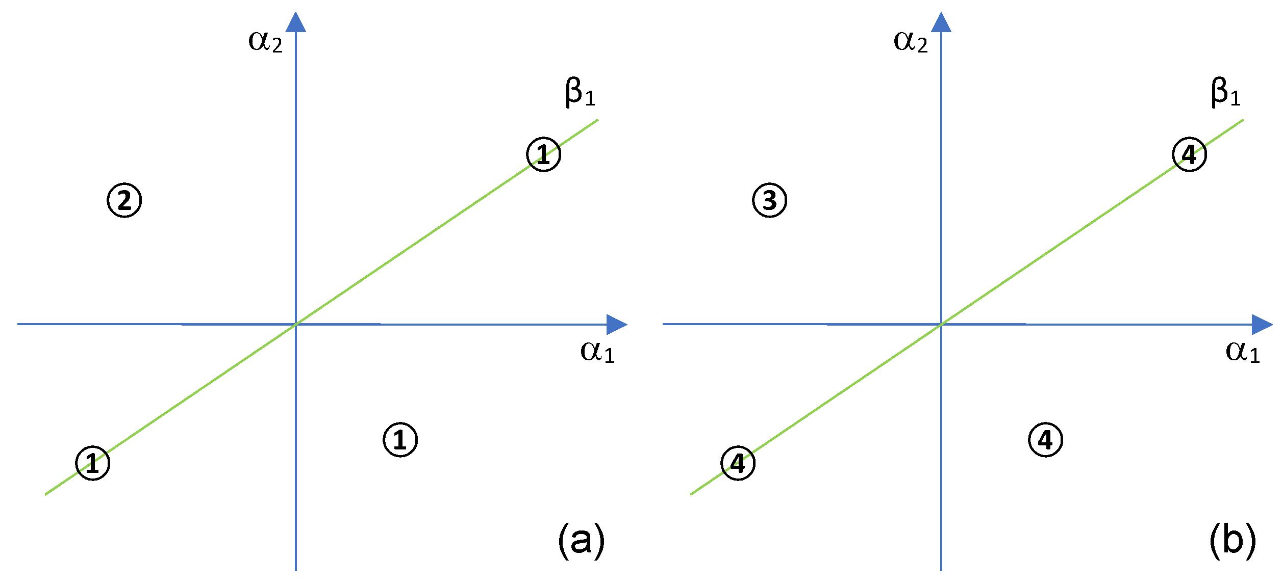
3.2. Degree of the Second Bifurcation Curve Is Two

If Deg β 2 = 2 , then its first three coefficients will be denoted as below.
β 1 ( α 1 , α 2 ) = a α 2 3 + b α 2 2 α 1 + c α 2 α 1 2 + d α 1 3 + O ( | α | 4 ) ,
β 2 ( α 1 , α 2 ) = h α 2 2 + k α 1 α 2 + l α 1 2 + O ( | α | 3 ) ,
where h , k , l R * .
Δ ( α 1 , α 2 ) = ( h α 2 2 + k α 1 α 2 + l α 1 2 ) 2 4 L 2 ( α ) [ a α 2 3 + b α 2 2 α 1 + c α 2 α 1 2 + d α 1 3 + O ( | α | 4 ) ]
= 4 L 0 ( a α 2 3 + b α 2 2 α 1 + c α 2 α 1 2 + d α 1 3 ) + O ( | α | 4 ) .
Truncated, that is:
β 1 ( α ) = a α 2 3 + b α 2 2 α 1 + c α 2 α 1 2 + d α 1 3
β 2 ( α ) = h α 2 2 + k α 1 α 2 + l α 1 2 ,
having Δ 2 = k 2 4 h l ,   Δ ( α ) = 4 L 0 β 1 ( α ) .
The sign of β 1 was previously analyzed.
The case when p and r are strictly negative and Δ 2 is strictly positive are considered below.
In the case p < 0 , r < 0 , Δ 2 > 0 , the polynomial β 1 ( T ) . This has the real roots e 1 < e 2 < e 3 (and the polynomial β 2 ( T ) has the real roots m 1 < m 2 ).
There are three cases that must be considered:
I
e 1 < m 1 < m 2 < e 2 < e 3 ;
II
e 1 < m 1 < e 2 < m 2 < e 3 ;
III
e 1 < m 1 < e 2 < e 3 < m 2 .
In each of those cases, there are four sub-cases depending on the signs of h and L 0 .
The bifurcation diagrams are given below, in Figure 4, Figure 5, Figure 6 and Figure 7.
The case when p, r, and Δ 2 are strictly negative is presented in the following.
In the case p < 0 , r < 0 , Δ 2 < 0 , we see that β 1 ( T ) has the real roots e 1 < e 2 < e 3 and β 2 ( T ) has no real roots ( Δ 2 < 0 ); therefore, s i g n β 2 ( α ) = s i g n ( h ) .
We know that s i g n δ ( α ) = s i g n ( L 0 ) s i g n β 1 ( α ) .
According to Lemma 1, (1), when p < 0 and r < 0 , the s i g n β 1 ( T ) = s i g n [ a ( T e 1 ) ( T e 2 ) ( T e 3 ) ] ; see Table 1.
From the information presented above, we obtain the following:
Remark 4.
When p < 0 , r < 0 , Δ 2 < 0 , the bifurcation diagrams are given in the following:
(1)
If a > 0 , h > 0 , L 0 > 0 or a < 0 , h > 0 , L 0 > 0 , then we get the Figure 8a.
(2)
If a > 0 , h > 0 , L 0 < 0 or a < 0 , h > 0 , L 0 < 0 , then we get the Figure 8b.
(3)
If a > 0 , h < 0 , L 0 > 0 or a < 0 , h < 0 , L 0 > 0 , then we get the Figure 9a.
(4)
If a > 0 , h < 0 , L 0 < 0 or a < 0 , h < 0 , L 0 < 0 , then we get the Figure 9b.
The case when p is strictly positive or (p is strictly negative and r is positive) will be investigated next.
In the case when p > 0 or ( p < 0 and r 0 ), from Lemma 1, (2) we have,
s i g n β 1 ( T ) = s i g n [ a ( T e 1 ) ] ,
see Table 2.
(a) There is one real root e 1 and two complex conjugates roots of β 1 ( T ) when r > 0 ;
(b) When p < 0 and r = 0 , there are three real roots, one simple e 1 and two common;
(c) Then p > 0 , q 0 , there is one real root e 1 and two complex conjugates;
(d) If p > 0 , q = 0 , there is a triple root e 1 .
From (a)–(d), we see that, in all these cases, β 1 ( T ) = 0 has a single real root e 1 and then s i g n β 1 ( T ) = s i g n [ a ( T e 1 ) ] .
Δ ( α ) = 4 L 0 β 1 ( α ) and then s i g n Δ ( α ) = s i g n ( L 0 ) s i g n [ β 1 ( α ) ] .
For the sign of β 2 ( α ) , we have two cases:
  • Δ 2 < 0 implies s i g n β 2 ( α ) = s i g n ( h ) ;
  • Δ 2 > 0 , then there is m 1 , m 2 , two distinct real roots of β 2 ( α ) = 0 and
    s i g n β 2 ( α ) = s i g n ( h ) , if m ( , m 1 ) ( m 2 , ) s i g n ( h ) , if m ( m 1 , m 2 ) .
Remark 5.
When p > 0 or ( p < 0 and r 0 ) and Δ 2 < 0 , then only two cases will appear:
  • If a > 0 , L 0 > 0 , h > 0 or a < 0 , L 0 > 0 , h > 0 , see Figure 10a;
  • If a > 0 , L 0 < 0 , h > 0 or a < 0 , L 0 < 0 , h > 0 , see Figure 10b;
  • If a > 0 , L 0 > 0 , h < 0 or a < 0 , L 0 > 0 , h < 0 , see Figure 11a;
  • If a > 0 , L 0 < 0 , h < 0 or a < 0 , L 0 < 0 , h < 0 , see Figure 11b.
When Δ 2 > 0 , we have e 1 , m 1 , m 2 , so we write the following situations: e 1 < m 1 < m 2 , m 1 < e 1 < m 2 , and m 1 < m 2 < e 1 . We notice that, in the case m 1 < m 2 < e 1 , the bifurcations diagrams will be obtained by a rotation from the bifurcation diagrams obtained in the case e 1 < m 1 < m 2 because e 1 is not in the interval ( m 1 , m 2 ) . In addition, we will draw below only β 1 because the two lines of β 2 do not produce the changing of the region of bifurcation in this case.
Remark 6.
When Δ 2 > 0 and p > 0 or ( p < 0 and r 0 ), then the bifurcation diagrams will be obtained as in previous remark, as follows:
  • If e 1 < m 1 < m 2 and a > 0 , L 0 > 0 , h > 0 or a < 0 , L 0 > 0 , h > 0 or if m 1 < e 1 < m 2 and a > 0 , L 0 > 0 , h < 0 or a < 0 , L 0 > 0 , h < 0 , then will obtain Figure 10a.
  • If e 1 < m 1 < m 2 and a > 0 , L 0 < 0 , h > 0 or a < 0 , L 0 < 0 , h > 0 or if m 1 < e 1 < m 2 and a > 0 , L 0 < 0 , h < 0 or a < 0 , L 0 < 0 , h < 0 , then will obtain Figure 10b.
  • If e 1 < m 1 < m 2 and a > 0 , L 0 > 0 , h < 0 or a < 0 , L 0 > 0 , h < 0 or if m 1 < e 1 < m 2 and a > 0 , L 0 > 0 , h < 0 or a < 0 , L 0 > 0 , h > 0 , then will obtain Figure 11a.
  • If e 1 < m 1 < m 2 and a > 0 , L 0 < 0 , h < 0 or a < 0 , L 0 < 0 , h > 0 or if m 1 < e 1 < m 2 and a > 0 , L 0 < 0 , h > 0 or a < 0 , L 0 < 0 , h < 0 , then will obtain Figure 11b.

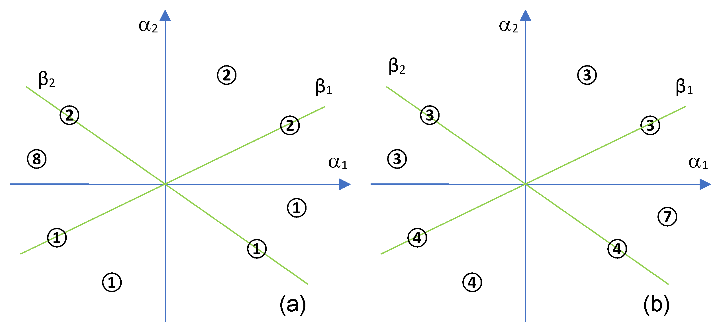
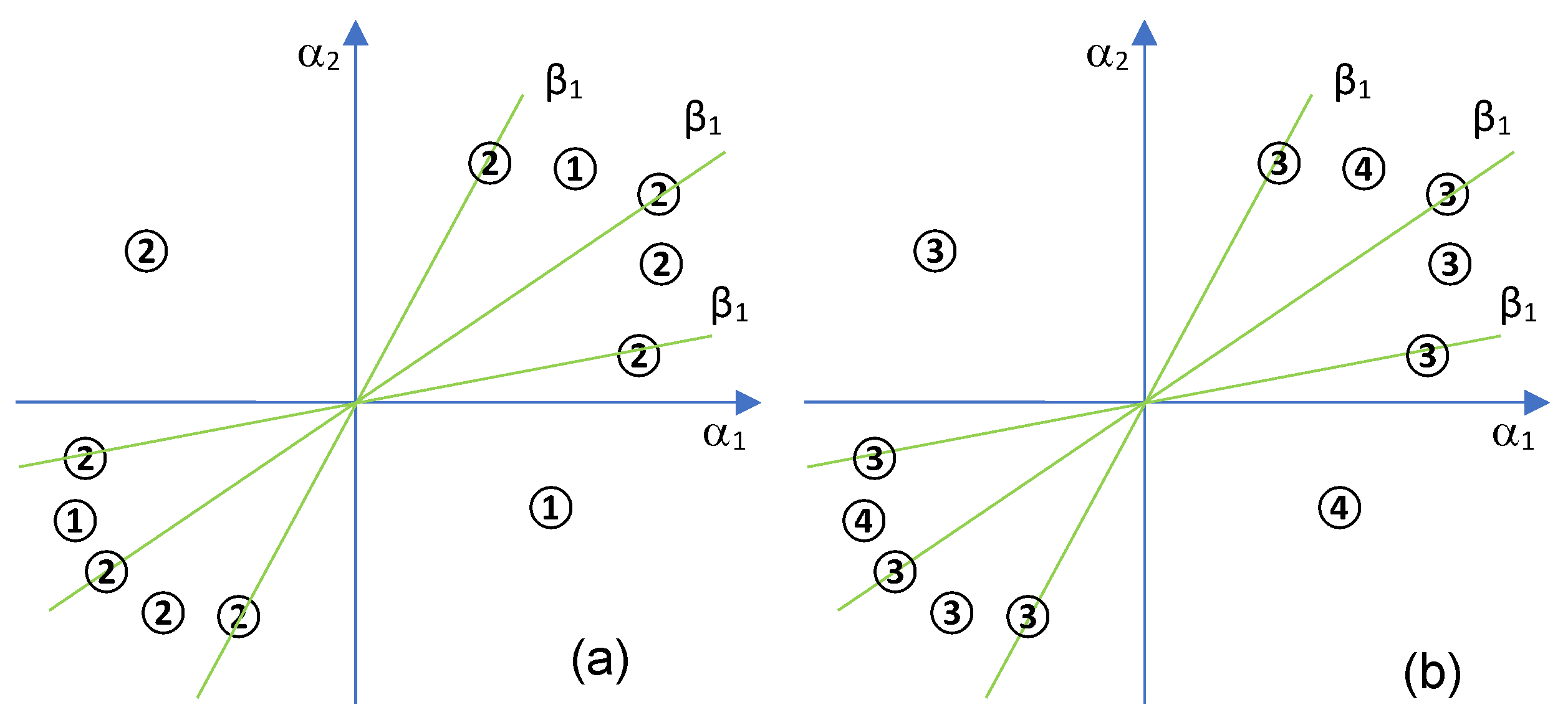
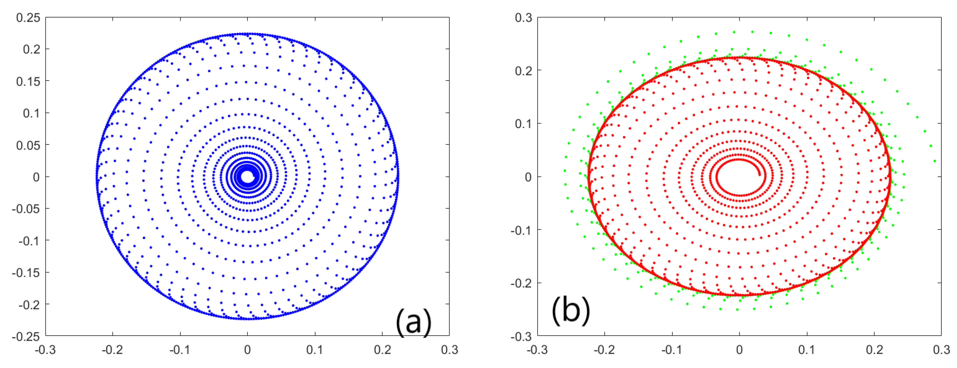
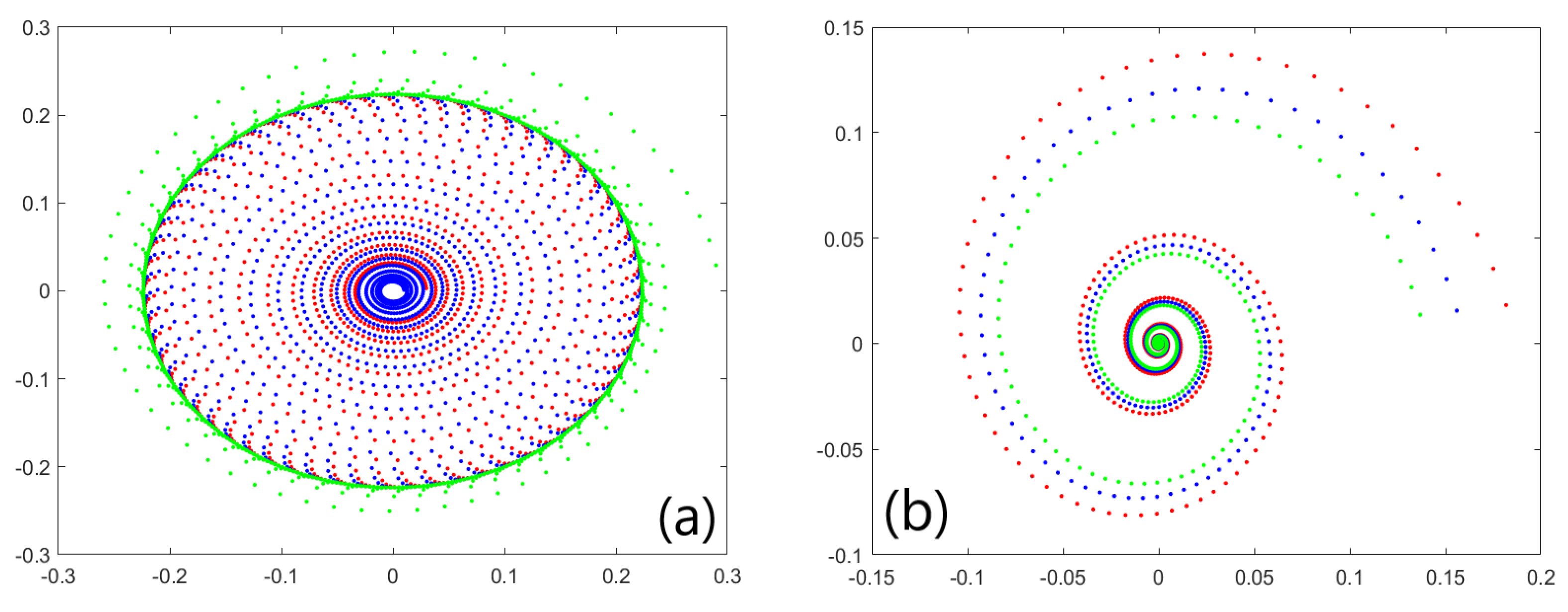
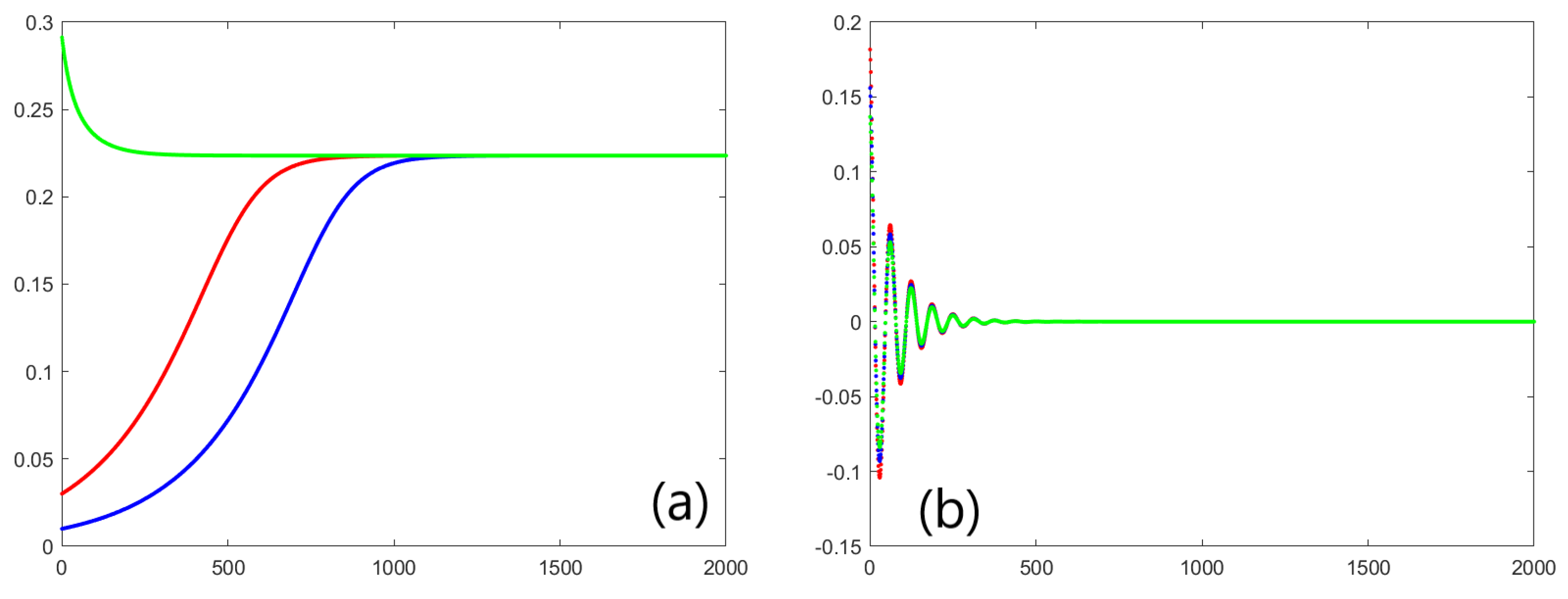
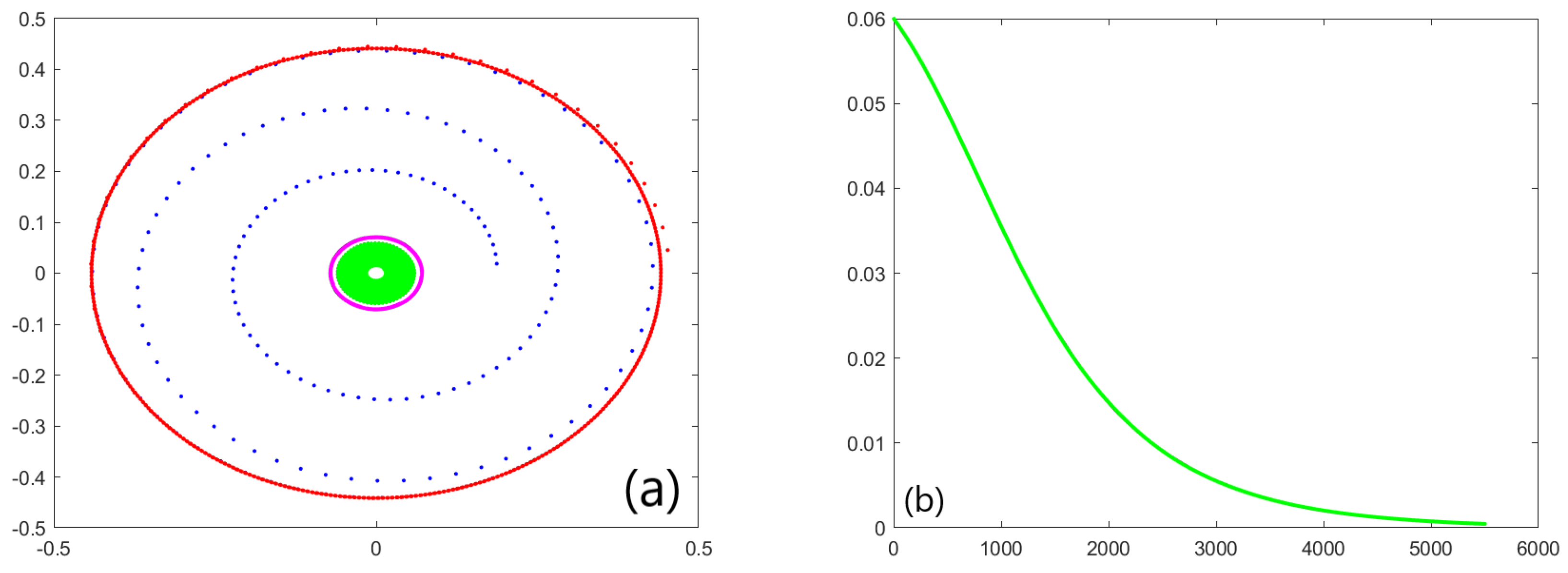
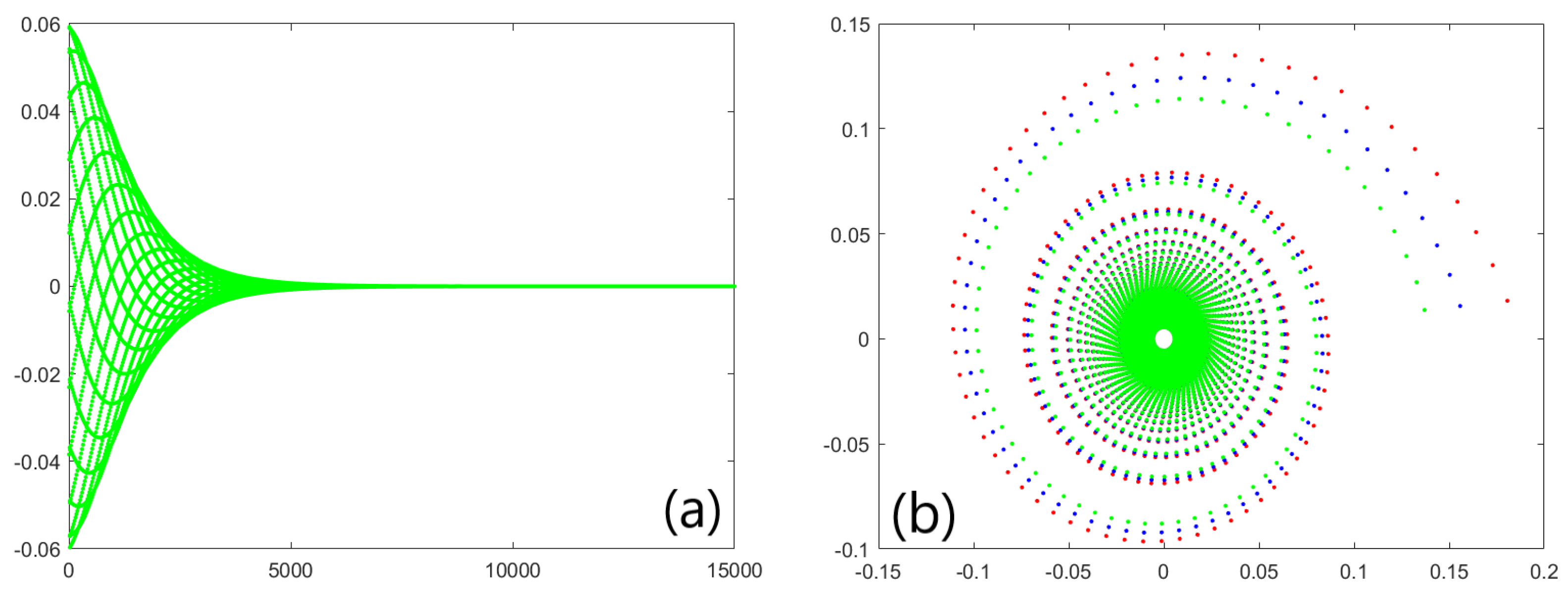
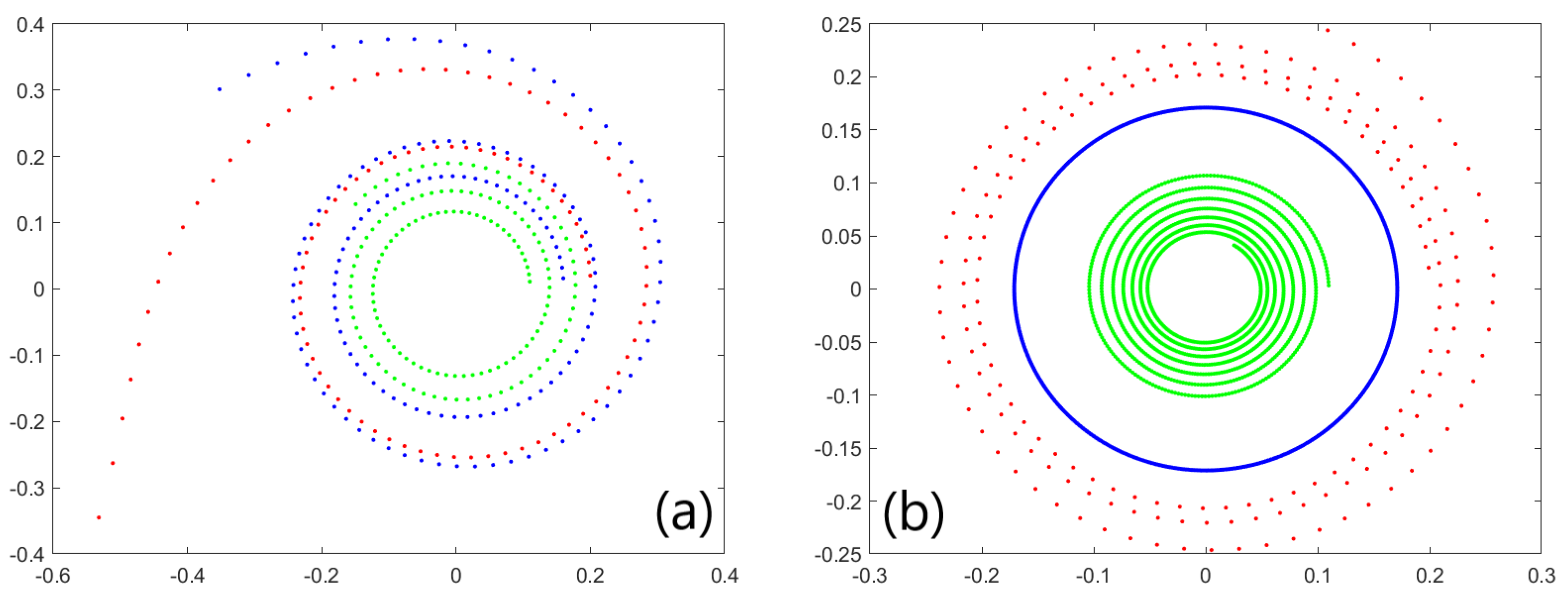
3.3. Numerical Simulations

Some numerical examples are given below in order to illustrate the theoretical approach. Matlab simulations are presented for the regions in Figure 11b, but first we have to check the conditions of Remark 5, i.e., p > 0 , Δ 2 < 0 , and a > 0 , L 0 < 0 , h < 0 for the example given below. Considering β 1 ( α ) = 2 α 1 3 + α 2 + α 1 2 α 2 , β 2 ( α ) = ( α 1 2 + α 1 α 2 + α 2 2 ) , with | α | being sufficiently small and θ 0 = 0.1, L 0 = 1 , we notice that a = 1 , b = 0 , c = 1 , d = 2 , h = 1 , k = 2 , l = 1 , and p = 1 > 0 , Δ 2 < 0 , a > 0 , h < 0 . We find different orbits ( x n , y n ) , where x n = ρ n sin φ n , x n = ρ n cos φ n , when n = 1 , , N , N being a fixed number. Then the two-dimensional map, in polar coordinates, becomes,
ρ n + 1 = ρ n + ρ n β 1 ( α ) + ρ n 3 β 2 ( α ) ρ n 5 , φ n + 1 = φ n + θ 0 .
It is obvious that the Chenciner bifurcation is degenerated here.
Figure 12a,b and Figure 13a give the generic portrait phase 3, and Figure 13b gives the generic portrait phase 4.
First consider α 1 = 0.1, α 2 = 0.1, N = 2000 , and ( ρ 1 , φ 1 ) = ( 0.3, 0 ) (for green curve), ( ρ 1 , φ 1 ) = ( 0.01, 0 ) (for blue curve), and ( ρ 1 , φ 1 ) = ( 0.03, 0 ) (for red curve), respectively; the discrete orbits can be seen in Figure 12a,b and Figure 13a. The orbits for blue, red, and green curves tend to an invariant stable closed curve. Moreover, in Figure 14a, the red, blue, and green sequence of points represent the ρ n sequence corresponding to the previous three orbits, respectively, when N = 2000 in ( n O ρ n ) axis. We can notice that the results from Figure 12 and Figure 13a are checked because ρ n tends to the same constant number when n tends to infinity, and then the orbits will be on the same circle. In Figure 14b, the red, blue, and green sequence of points represent the ρ n sequence corresponding to previous three orbits, respectively, when N = 2000 in ( n O ρ n ) axis. This time, these sequences tend to zero, so the three orbits tend to origin and the result from Figure 13b is checked. Here, α 1 = 0.5, α 2 = 0.513, N = 2000 are taken, and the start points are the same as in Figure 13b. It can be observed that the orbit tends to the origin, therefore region 4 will appear; see Figure 13b.
Now choosing β 1 ( α ) = α 1 3 + 2 α 2 3 α 1 α 2 2 α 1 2 α 2 , β 2 ( α ) = α 1 3 α 2 , α 1 = 0.1 , α 2 = 0.1 , and ( ρ 1 , φ 1 ) = ( 0.06) , N = 700 , the orbit (green color) tends to origin and will depart from the inner invariant curve (magenta color). However, when ( ρ 1 , φ 1 ) = ( 0.187, 0 ) , the orbit (blue color) will tend from interior to the outer invariant curve (red color). When ( ρ 1 , φ 1 ) = ( 0.3, 0 ) , the orbit (in red) will tend from exterior to the outer invariant curve. Thus, here, in Figure 15a, appears the phase portrait for the region 7, see Appendix A, and this is confirmed also from theoretical conditions from Figure 2b. In Figure 15b, the sequence ρ n in ( n O ρ n ) axis is shown for green orbit from Figure 15a, where N = 6000 , observing that this sequence tends to zero when n tends to infinity. In Figure 16a, the sequence x n is given in the axis ( n O x n ) , for N = 15,000, and also tends to zero.
In Figure 16b is considered the case when ( α 1 , α 2 ) = ( 0.9, 0.9) are on β 1 ( α ) = 0 . Here β 1 ( α ) = 2 α 1 3 + α 2 3 + α 1 2 α 2 , β 2 ( α ) = α 1 2 α 1 α 2 α 2 2 , θ 0 = 0.1 . Now β 1 ( α 1 , α 2 ) = 0 , but Δ 2 < 0 and ( ρ 1 , φ 1 ) = ( 0.187, 0 ) for red orbit, ( ρ 1 , φ 1 ) = ( 0.16, 0 ) for blue orbit, and ( ρ 1 , φ 1 ) = ( 0.14, 0 ) for green orbit, respectively, which tend to the origin. Therefore, the region 4 corresponds to the phase portrait, see Figure 11b, this being the third and last case analyzed for Figure 11b.
Moreover, in Figure 17a,b appear the phase portraits 2 and 1 from Figure 11a, when p > 0 , a > 0 , L 0 > 0 , h < 0 for the map,
ρ n + 1 = ρ n + ρ n β 1 ( α ) + ρ n 3 β 2 ( α ) + ρ n 5 , φ n + 1 = φ n + θ 0 ,
i.e., L 0 = 1 . Here we take θ 0 = 0.1, β 1 ( α ) = 2 α 1 3 + α 2 3 + α 1 2 α 2 , β 2 ( α ) = α 1 2 α 2 2 α 1 α 2 , and α 1 = 0.1, α 2 = 0.1 for Figure 17a. The starting points of the three orbits correspond to ( ρ 1 , φ 1 ) = ( 0.2, 0 ) for the red color, ( ρ 1 , φ 1 ) = ( 0.16, 0 ) for the blue color, and ( ρ 1 , φ 1 ) = ( 0.11, 0 ) for the green color, respectively, and N = 100 step for the red orbit and N = 150 step for the blue and green orbits. The orbits depart from the origin and escape to infinity. This situation corresponds to phase portrait 2.
When α 1 = 0.1, α 2 = 0.112 , and the same starting points are taken for the red and green orbits, but θ 0 = 0.003 , N = 1500 for the blue and green orbits, and, for the blue orbit, ( ρ 1 , φ 1 ) = ( 0.1711, 0 ) , N = 200 , and θ 0 = 0.1 , then the red orbit departs from the invariant circle, which is the blue orbit, and the green orbit departs from the invariant circle and tends to origin. That corresponds to the phase portrait 1, and this happens in region 1 from Figure 11a.

4. Discussions and Conclusions

This paper contributes to the enrichment of the literature related to the Chenciner bifurcation. This study may be useful in biology, medicine, and economics, where discrete Chenciner bifurcation occurs.
The degeneracy case of the Chenciner bifurcation written in the truncated normal form, which was analyzed here, takes place when a 20 = a 11 = a 02 = 0 , and for b 10 and b 01 , we have two situations: b 10 0 , b 01 0 or b 10 = b 01 = 0 . This is a further degeneration of β 1 . It appears here a symmetry and an asymmetry of some regions from bifurcation diagrams in this case studied.
The proposed approach is different from that of [28], being similar to that of [26,27], solving the problem in a more general framework than in [28]. This paper continues the study realized in [26,27], which is shortly described in Appendix A and Appendix B, by considering the following new assumption a 10 = a 01 = a 20 = a 11 = a 02 = 0 . A different method is necessary than that used in [26], based on the sign of Δ and Δ 2 when degree of β 1 ( α ) is three and degree of β 2 ( α ) is one or two.
This article highlights 18 different bifurcation diagrams, which is more than the two obtained in the case of non-degeneration [25]. Those 18 different bifurcation diagrams come from the first case, Case 3.1, when Deg β 1 ( α ) = 3 and Deg β 2 ( α ) = 1 , here having six bifurcation diagrams, and from the second case, Case 3.2, when Deg β 1 ( α ) = 3 and Deg β 2 ( α ) = 2 , where 12 different bifurcation diagrams appear. The study we conducted in this article confirms the hypothesis. Therefore, in a case of degeneration that does not involve resonance, there is an increase in the number of bifurcation diagrams. This study answers a part of the open problem from [26], and a new open problem would be to study the behavior of the system when D e g β 1 ( α ) = 3 and D e g β 2 ( α ) = 3 in the truncated form.
There are more cases of possible degeneration of Chenciner bifurcation, and each of them requires a special characteristic method of solving, especially developed for each case. Matlab simulations verify the theoretical conclusions.

Author Contributions

Conceptualization, S.L. and L.C.; formal analysis, S.L., L.C., and E.G.; investigation, S.L., L.C., and E.G.; methodology, S.L. and L.C.; resources, L.C. and E.G.; data curation, L.C. and E.G.; writing—original draft preparation, L.C.; writing—review and editing, L.C.; visualization, S.L., L.C., and E.G.; supervision, S.L., L.C., and E.G.; project administration, S.L., L.C., and E.G.; funding acquisition, L.C. and E.G. All authors have read and agreed to the published version of the manuscript.

Funding

This research received no external funding.

Institutional Review Board Statement

Not applicable.

Informed Consent Statement

Not applicable.

Data Availability Statement

Data sharing not applicable.

Acknowledgments

This research was partially supported by the Horizon 2020-2017-RISE-777911 project.

Conflicts of Interest

The authors declare no conflict of interest.

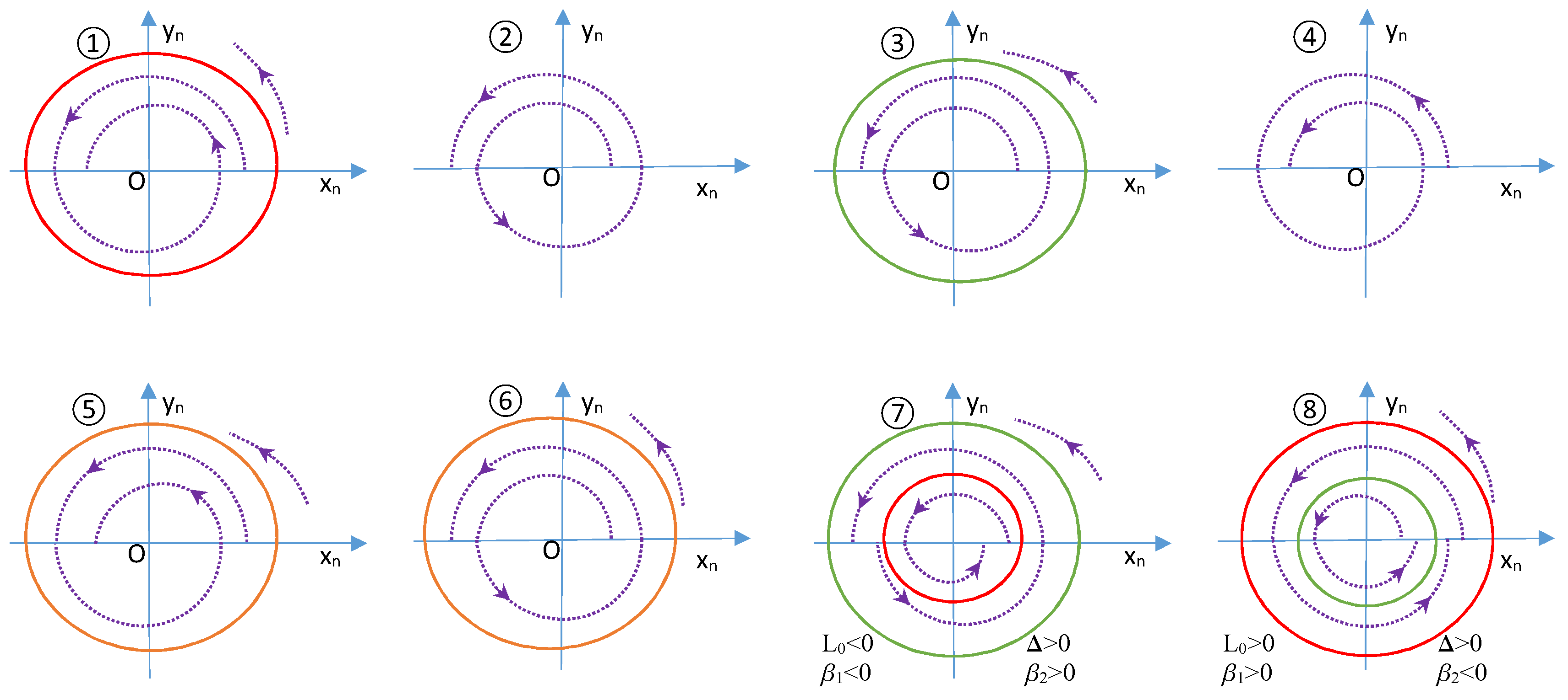
Appendix A. Chenciner Bifurcations

Below is written the normal form of Neimark-Sacker bifurcation with cubic degeneracy, i.e., Chenciner bifurcation for the system (A1). A discrete dynamical system:“
x n + 1 = f x n , α
with α = α 1 , α 2 R 2 , x n R 2 , n N , f C r , and r 2 can be written as
x f x , α
[26].” By using the same methods as in [25,26,27], (A2) becomes
z μ α z + g z , z ¯ , α ,
and“
w r α e i θ α + a 1 α w w ¯ + a 2 α w 2 w ¯ 2 w + O w 6 = r α + b 1 α w w ¯ + b 2 α w 2 w ¯ 2 w e i θ α + O w 6
respectively, taking into account that g can be written as
g z , z ¯ , α = k + l 2 1 k ! l ! g k l α z k z ¯ l ,
where μ , g , g k l α are smooth functions, b k α = a k α e i θ α , k = 1 , 2 . , μ α = r α e i θ α , r 0 = 1 , and θ 0 = θ 0 ” [26]. The following notations were used:
β 1 α = r α 1 and β 2 α = R e b 1 ( α )
in [26,27] and (A4) was“
ρ n + 1 = ρ n 1 + β 1 α + β 2 α ρ n 2 + L 2 α ρ n 4 + ρ n O ρ n 6 φ n + 1 = φ n + θ α + ρ n 2 I m b 1 α β 1 α + 1 + O ρ n , α ,
L 2 α = I m 2 b 1 α + 2 1 + β 1 α R e b 2 α 2 β 1 α + 1 ” [26,27,28]).
When r 0 = 1 , R e b 1 ( 0 ) = 0 , but L 2 0 0 in (A6), the generalized Neimark–Sacker bifurcation appears and the transformation of parameters
α 1 , α 2 β 1 α , β 2 α
is regular at 0 , 0 . These types of bifurcations have been studied in [25], and there they are called Chenciner bifurcations. It is easy to see from above that, for β 1 0 = 0 , we have L 2 0 = 1 2 I m 2 b 1 0 + 2 R e b 2 0 . The idea is “to change these coordinates and to work only using the initial parameters ( α 1 , α 2 ) in the form (A6)” [26].
It is known from [26], relation (13), page 4 that
β 1 ( α ) = i + j = 1 p a i j α 1 i α 2 j + O ( | α | p + 1 ) , β 2 ( α ) = i + j = 1 q b i j α 1 i α 2 j + O ( | α | q + 1 )
for p , q 1 , a 10 = β 1 α 1 | α = 0 , a 01 = β 1 α 2 | α = 0 , b 01 = β 2 α 2 | α = 0 , b 10 = β 2 α 1 | α = 0 , and so on.
The transformation (A7) is not regular at 0 , 0 , i.e., the Chenciner bifurcation degenerates, if and only if
a 10 b 01 a 01 b 10 = 0 .
Knowing the “truncated form of the ρ -map of (A6),
ρ n + 1 = ρ n 1 + β 1 α + β 2 α ρ n 2 + L 2 α ρ n 4 ,
the φ -map of the system (A6) describes a rotation by an angle depending on α and ρ and can be approximated by,
φ n + 1 = φ n + θ α ,
being assumed that 0 < θ 0 < π ” [26]. The truncated normal form of (A4) is (A10) and (A11).

Appendix B. Literature Review
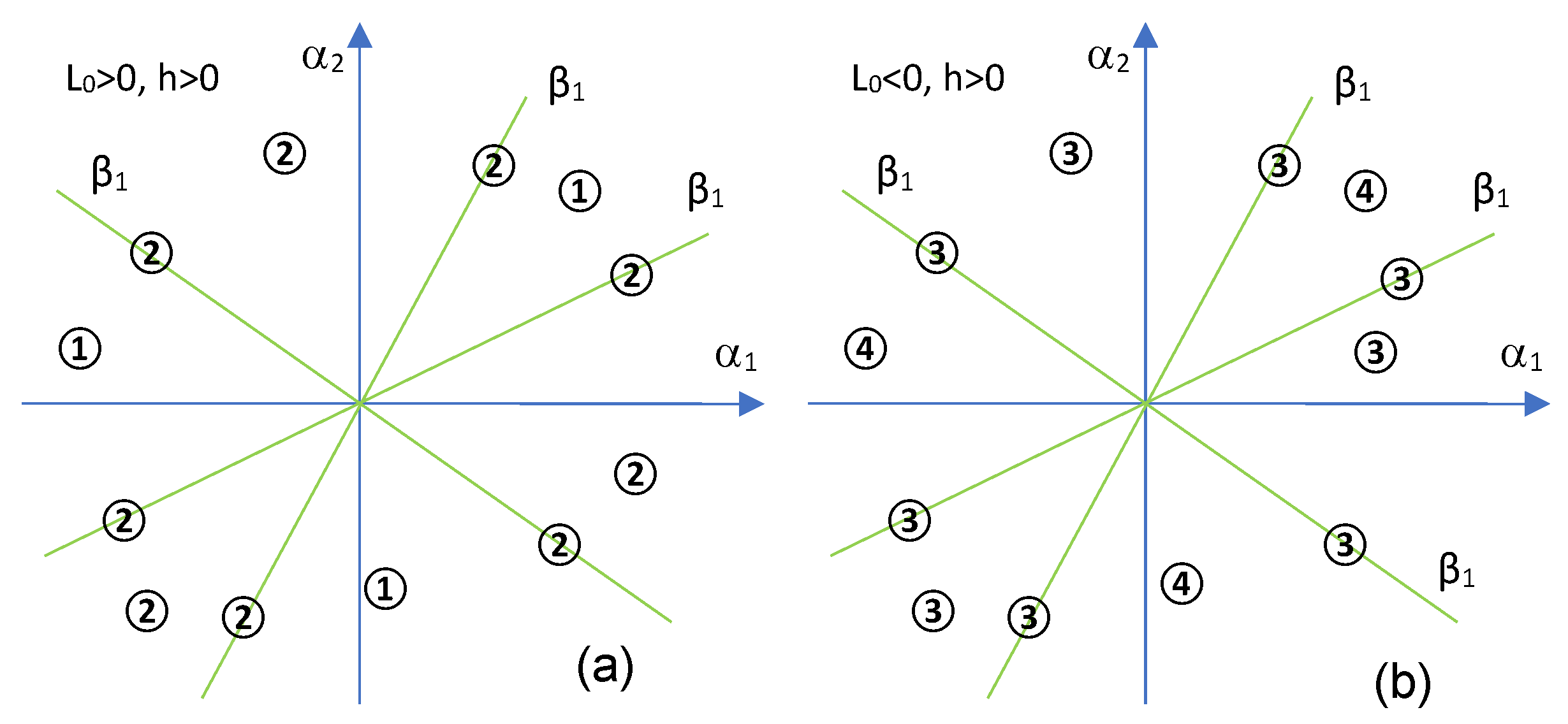
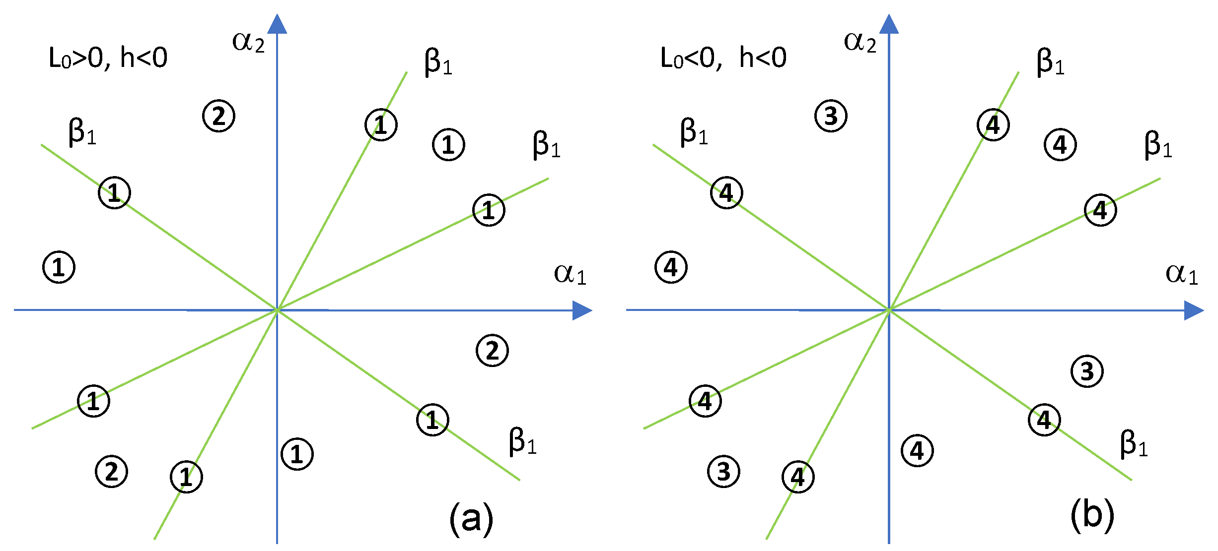
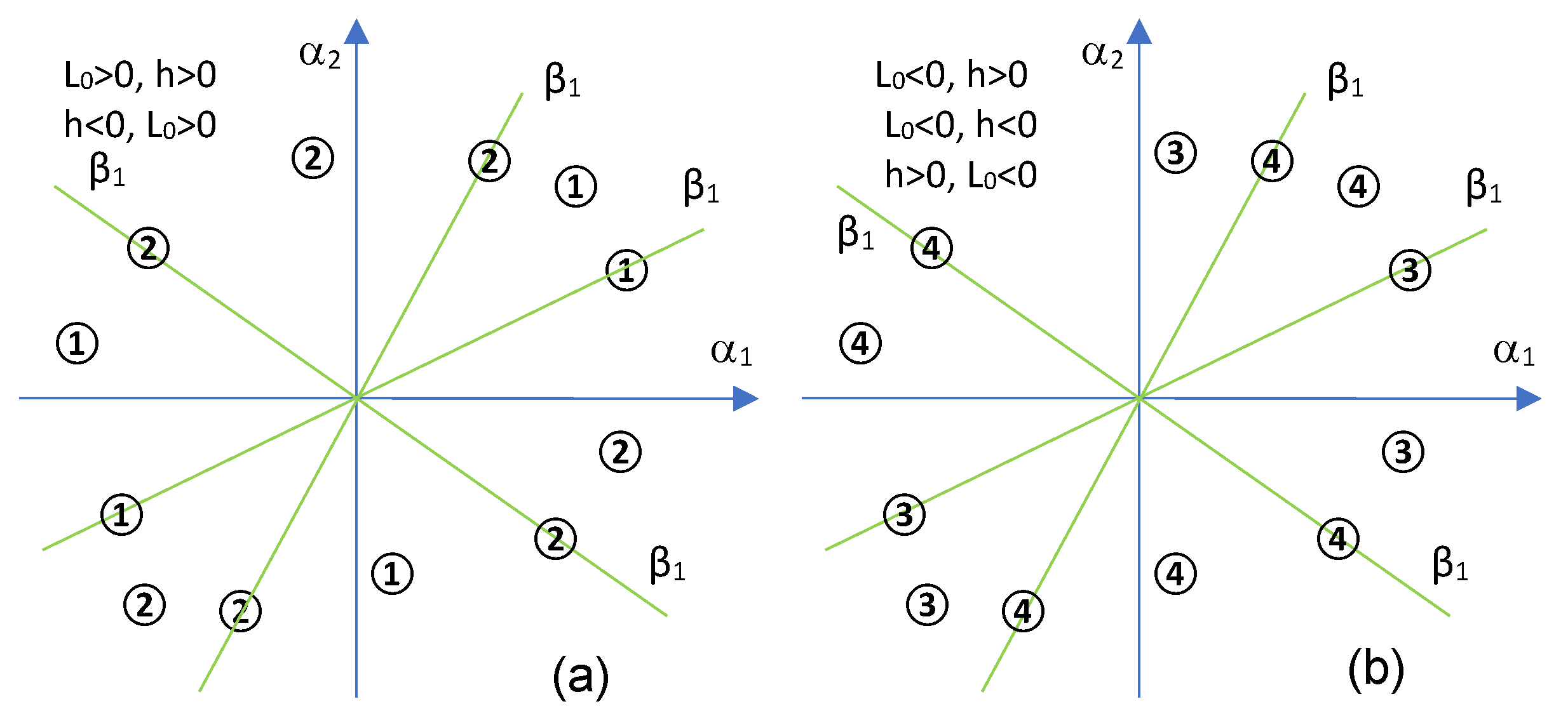
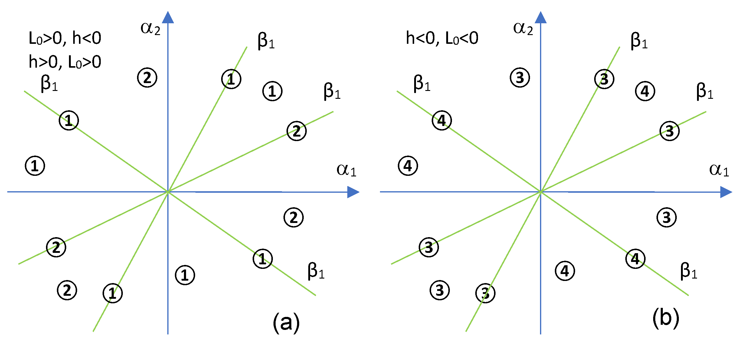
It is known that “the one dimensional dynamic system for the ρ -map (A10) has a fixed point in origin for all values of α , which corresponds to the fixed point O(0, 0) in the system (A10) and (A11), and that a positive nonzero fixed point of the one-dimensional ρ -map (A10), corresponds to a closed invariant curve in the truncated two-dimensional map (A10)–(A11)” [26].
On the other hand, s i g n L 2 α = s i g n L 0 for α = α 1 2 + α 2 2 sufficiently small because L 2 α = L 0 1 + O α and L 0 0 . It is considered O α n for n 1 to be the series, O α n = i + j n c i j α 1 i α 2 j .
Theorem A1.
The fixed point O is (linearly) stable if β 1 α < 0 and unstable if β 1 α > 0 , for all values α with α sufficiently small. On the bifurcation curve β 1 α = 0 , O is (non-linearly) stable if β 2 α < 0 and unstable if β 2 α > 0 , when α is sufficiently small. At α = 0 , O is (non-linearly) stable if L 0 < 0 and unstable if L 0 > 0 [26].
The positive nonzero fixed points of (A10) are solutions of the following equation:
L 2 α y 2 + β 2 α y + β 1 α = 0
where y = ρ n 2 . The roots of (A12) will be denoted by y 1 = 1 2 L 2 Δ β 2 and y 2 = 1 2 L 2 Δ + β 2 when these roots are real, and Δ α = β 2 2 α 4 β 1 α L 2 α [26].
Theorem A2.
“(1) When Δ α < 0 for all α sufficiently small, the system (A10) and (A11) has no invariant circles.
(2) When Δ α > 0 for all α sufficiently small, the system (A10) and (A11) has:
(a)
one invariant unstable circle ρ n = y 1 if L 0 > 0 and β 1 α < 0 ;
(b)
one invariant stable circle ρ n = y 2 if L 0 < 0 and β 1 α > 0 ;
(c)
two invariant circles, ρ n = y 1 unstable and ρ n = y 2 stable, if L 0 > 0 , β 1 α > 0 , β 2 α < 0 or L 0 < 0 , β 1 α < 0 , β 2 α > 0 ; in addition, y 1 < y 2 if L 0 < 0 and y 2 < y 1 if L 0 > 0 ;
(d)
no invariant circles if L 0 > 0 , β 1 α > 0 , β 2 α > 0 or L 0 < 0 , β 1 α < 0 , β 2 α < 0 .
(3) On the bifurcation curve Δ α = 0 , the system (A10) and (A11) has one invariant unstable circle ρ n = y 1 for all L 0 0 . Moreover, if L 0 < 0 , the invariant circle is stable from the exterior and unstable from the interior, while if L 0 > 0 it is vice versa.
(4) When β 1 α = 0 , the system (A10) and (A11) has one invariant circle ρ n = β 2 α L 0 whenever L 0 β 2 α < 0 . It is stable if L 0 < 0 and β 2 α > 0 , respectively, unstable if L 0 > 0 and β 2 α < 0 ” [26,27,28].
Corresponding to the studies we have carried out previously [26,27], the following phase portraits can be highlighted below. In this case, the phase portraits for the curves of bifurcation when Δ ( α ) = 0 are shown.
Figure A1. Generic portraits phase when θ 0 > 0 .
Mathematics 10 01603 g0a1

References

  1. Sanchez-Ruiz, L.M.; Moll-Lopez, S.; Morano-Fernandez, J.A.; Rosello, M.D. Dynamical Continuous Discrete Assessment of Competencies Achievement: An Approach to Continuous Assessment. Mathematics 2021, 9, 2082. [Google Scholar] [CrossRef]
  2. Elhassan, C.; Zulkifli, S.A.; Iliya, S.Z.; Bevrani, H.; Kabir, M.; Jackson, R.; Khan, M.H.; Ahmed, M. Deadbeat Current Control in Grid-Connected Inverters: A Comprehensive Discussion. IEEE Access 2022, 10, 3990–4014. [Google Scholar] [CrossRef]
  3. Chang, X.H.; Jin, X. Observer-based fuzzy feedback control for nonlinear systems subject to transmission signal quantization. Appl. Math. Comput. 2022, 414, 126657. [Google Scholar] [CrossRef]
  4. Park, S.J.; Cho, K.H. Discrete Event Dynamic Modeling and Analysis of the Democratic Progress in a Society Controlled by Networked Agents. IEEE Trans. Autom. Control 2022, 1, 359–365. [Google Scholar] [CrossRef]
  5. Sukhinov, A.; Belova, Y.; Chistyakov, A.; Beskopylny, A.; Meskhi, B. Mathematical Modeling of the Phytoplankton Populations Geografic Dynamics for Possible Scenarios of Changes in the Azov Sea Hydrological Regime. Mathematics 2021, 9, 3025. [Google Scholar] [CrossRef]
  6. Niu, L.; Ruiz-Herrera, A. Simple dynamics in non-monotone Kolmogorov systems. Proc. R. Soc. Edinb. Sect. A-Math. 2021, 1–16. [Google Scholar] [CrossRef]
  7. Wang, X.; Lu, J.; Wang, Z.; Li, Y. Dynamics of discrete epidemic models on heterogeneous networks. Physica A 2020, 539, 122991. [Google Scholar] [CrossRef]
  8. Abdel-Gawad, H.I.; Abdel-Gawad, A.H. Discrete and continuum models of COVID-19 virus, formal solutions, stability and comparison with real data. Math. Comput. Simul. 2021, 190, 222–230. [Google Scholar] [CrossRef]
  9. Miranda, L.K.A.; Kuwana, C.M.; Huggler, Y.H.; da Fonseca, A.K.P.; Yoshida, M.; de Oliveira, J.A.; Leonel, E.D. A short review of phase transition in a chaotic system. Eur. Phys. J.-Spec. Top. 2021, 1–11. [Google Scholar] [CrossRef]
  10. Nordmark, A.B. Non-periodic motion caused by grazing incidence in an impact oscillator. J. Sound Vib. 1991, 145, 279–297. [Google Scholar] [CrossRef]
  11. Water, W.; Molenaar, J. Dynamics of vibrating atomic force microscopy. Nanotechnology 2000, 11, 192–199. [Google Scholar] [CrossRef]
  12. Molenaar, J.; Weger, J.G.; Water, W. Mappings of grazing-impact oscillators. Nonlinearity 2001, 14, 301–321. [Google Scholar] [CrossRef]
  13. Mercinger, M.; Fercec, B.; Oliveire, R.; Pagon, D. Cyclicity of some analytic maps. Appl. Math. Comput. 2017, 295, 114–125. [Google Scholar]
  14. Yao, W.B.; Li, X.Y. Complicate bifurcation behaviors of a discrete predator-prey model with group defense and nonlinear harvesting in prey. Appl. Anal. 2022, 1–16. [Google Scholar] [CrossRef]
  15. Akrami, M.H.; Atabaigi, A. Dynamics and Neimark-Sacker Bifurcation of a Modified Nicholson-Bailey Model. J. Math. Ext. 2022, 16, 1–18. [Google Scholar]
  16. Deng, S.F. Bifurcations of a Bouncing Ball Dynamical System. Int. Bifurc. Chaos 2019, 29, 1950191. [Google Scholar] [CrossRef]
  17. Lines, M.; Westerhoff, F. Effects of inflation expectations on macroeconomics dynamics:extrapolative versus regressive expectations. Stud. Nonlinear Dyn. Econom. 2012, 16, 7. [Google Scholar] [CrossRef] [Green Version]
  18. Neugart, M.; Tuinstra, J. Endogenous fluctuations in the demand for education. J. Evol. Econ. 2003, 13, 29–51. [Google Scholar] [CrossRef] [Green Version]
  19. Palan, S. A Review of Bubbles and Crashes in Experimental Asset Markets. J. Econ. Surv. 2013, 27, 570–588. [Google Scholar] [CrossRef]
  20. Agliari, A.; Hommes, C.H.; Pecora, N. Path dependent coordination of expectations in asset pricing experiments: A behavioral explanation. J. Econ. Behav. Organ. 2016, 121, 15–28. [Google Scholar] [CrossRef] [Green Version]
  21. Chenciner, A. Bifurcations de points fixes elliptiques. III. Orbites periodiques de “petites periodes” et elimination resonnante des couples de courbes invariantes. Inst. Hautes Etudes Sci. Publ. Math. 1988, 66, 5–91. [Google Scholar] [CrossRef]
  22. Chenciner, A. Bifurcations de points fixes elliptiques. I. Courbes invariantes. IHES-Publ. Math. 1985, 61, 67–127. [Google Scholar] [CrossRef]
  23. Chenciner, A. Bifurcations de points fixes elliptiques. II. Orbites periodiques et ensembles de Cantor invariants. Invent. Math. 1985, 80, 81–106. [Google Scholar] [CrossRef]
  24. Arrowsmith, D.; Place, C. An Introduction to Dynamical Systems; Cambridge University Press: Cambridge, UK, 1990. [Google Scholar]
  25. Kuznetsov, Y.A. Elements of Applied Bifurcation Theory, 3rd ed.; Springer: New York, NY, USA, 2004. [Google Scholar]
  26. Tigan, G.; Lugojan, S.; Ciurdariu, L. Analysis of Degenerate Chenciner Bifurcation. Int. J. Bifurc. Chaos 2020, 30, 2050245. [Google Scholar] [CrossRef]
  27. Lugojan, S.; Ciurdariu, L.; Grecu, E. New Elements of analysis of a degenerate Chenciner bifurcation. Symmetry 2022, 14, 77. [Google Scholar] [CrossRef]
  28. Tigan, G.; Brandibur, O.; Kokovics, E.A.; Vesa, L.F. Degenerate Chenciner Bifurcation Revisited. Int. J. Bifurc. Chaos 2021, 31, 2150160. [Google Scholar] [CrossRef]
Figure 1. Bifurcation diagrams when p < 0 , r < 0 , and h k > 0 : (a) L 0 > 0 , k > 0 ; (b) L 0 > 0 , k < 0 .
Mathematics 10 01603 g001
Figure 2. Bifurcation diagrams when p < 0 , r < 0 , and h k > 0 : (a) L 0 < 0 , k > 0 ; (b) L 0 < 0 , k < 0 .
Mathematics 10 01603 g002
Figure 3. Bifurcation diagrams when p > 0 or ( p < 0 and r > 0 ) and h k > 0 : (a) a > 0 , k > 0 , L 0 > 0 or a > 0 , k < 0 , L 0 > 0 or a < 0 , k > 0 , L 0 > 0 or a < 0 , k < 0 , L 0 > 0 ; (b) a > 0 , k > 0 , L 0 < 0 or a > 0 , k < 0 , L 0 < 0 or a < 0 , k > 0 , L 0 < 0 or a < 0 , k < 0 , L 0 < 0 .
Mathematics 10 01603 g003
Figure 4. Bifurcation diagrams in the Case I when p < 0 , r < 0 , and Δ 2 > 0 : (a) L 0 > 0 , h > 0 ; (b) L 0 < 0 , h > 0 .
Mathematics 10 01603 g004
Figure 5. Bifurcation diagrams in the Case I when p < 0 , r < 0 , and Δ 2 > 0 : (a) L 0 > 0 , h < 0 ; (b) L 0 < 0 , h < 0 .
Mathematics 10 01603 g005
Figure 6. Bifurcation diagrams in the Case II and III when p < 0 , r < 0 , and Δ 2 > 0 : (a) L 0 > 0 , h > 0 or h < 0 , L 0 > 0 ; (b) L 0 < 0 , h > 0 or L 0 < 0 , h < 0 or h > 0 , L 0 < 0 .
Mathematics 10 01603 g006
Figure 7. Bifurcation diagrams in the Case II and III when p < 0 , r < 0 , and Δ 2 > 0 : (a) L 0 > 0 , h < 0 or h > 0 , L 0 > 0 ; (b) h < 0 , L 0 < 0 .
Mathematics 10 01603 g007
Figure 8. Bifurcation diagrams when p < 0 , r < 0 , and Δ 2 < 0 : (a) a > 0 , h > 0 , L 0 > 0 or a < 0 , h > 0 , L 0 > 0 ; (b) a > 0 , h > 0 , L 0 < 0 or a < 0 , h > 0 , L 0 < 0 .
Mathematics 10 01603 g008
Figure 9. Bifurcation diagrams when p < 0 , r < 0 , and Δ 2 < 0 : (a) a > 0 , h < 0 , L 0 > 0 or a < 0 , h < 0 , L 0 > 0 ; (b) a > 0 , h < 0 , L 0 < 0 or a < 0 , h < 0 , L 0 < 0 .
Mathematics 10 01603 g009
Figure 10. Bifurcation diagrams when p > 0 or ( p < 0 and r > 0 ): (a) a > 0 , L 0 > 0 , h > 0 or a < 0 , L 0 > 0 , h > 0 ; (b) a > 0 , L 0 < 0 , h > 0 or a < 0 , L 0 < 0 , h > 0 .
Mathematics 10 01603 g010
Figure 11. Bifurcation diagrams when p > 0 or ( p < 0 and r > 0 ): (a) a > 0 , L 0 > 0 , h < 0 or a < 0 , L 0 > 0 , h < 0 ; (b) a > 0 , L 0 < 0 , h < 0 or a < 0 , L 0 < 0 , h < 0 .
Mathematics 10 01603 g011
Figure 12. Numerical simulation for the map (9) when β 1 ( α ) = 2 α 1 3 + α 2 3 + α 1 2 α 2 , β 2 ( α ) = α 1 2 α 1 α 2 α 2 2 , with α 1 = 0.1, α 2 = 0.1 : (a) blue orbit starts from ( ρ 1 , φ 1 ) = ( 0.01, 0 ) ; (b) red orbit starts from ( ρ 1 , φ 1 ) = ( 0.03, 0 ) .
Mathematics 10 01603 g012
Figure 13. Numerical simulation for the map (9) when β 1 ( α ) = 2 α 1 3 + α 2 3 + α 1 2 α 2 , β 2 ( α ) = α 1 2 α 1 α 2 α 2 2 : (a) the three orbits are represented here with ( ρ 1 , φ 1 ) = ( 0.01, 0 ) , ( ρ 1 , φ 1 ) = ( 0.03, 0 ) and ( ρ 1 , φ 1 ) = ( 0.3, 0 ) , respectively, and α 1 = 0.1, α 2 = 0.1 ; (b) the three orbits are represented here with ( ρ 1 , φ 1 ) = ( 0.183, 0 ) , ( ρ 1 , φ 1 ) = ( 0.16, 0 ) and ( ρ 1 , φ 1 ) = ( 0.14, 0 ) , respectively, and α 1 = 0.5 , α 2 = 0.513 .
Mathematics 10 01603 g013
Figure 14. The discrete sequence ρ n given by the map (9) in the plane ( n O ρ n ) when β 1 ( α ) = 2 α 1 3 + α 2 3 + α 1 2 α 2 , β 2 ( α ) = α 1 2 α 1 α 2 α 2 2 : (a) when ( ρ 1 , φ 1 ) = ( 0.01, 0 ) , ( ρ 1 , φ 1 ) = ( 0.03, 0 ) , ( ρ 1 , φ 1 ) = ( 0.284, 0 ) and a 1 = 0.1, a 2 = 0.1 ; (b) when starting points are as in Figure 13b.
Mathematics 10 01603 g014
Figure 15. Numerical simulations for the map (9) when β 1 ( α ) = α 1 3 + 2 α 2 3 α 1 α 2 2 α 1 2 α 2 , β 2 ( α ) = α 1 3 α 2 and ( α 1 , α 2 ) = ( 0.1, 0.1) : (a) four orbits corresponding to ( ρ 1 , φ 1 ) = ( 0.06, 0 ) (the orbit in red), ( ρ 1 , φ 1 ) = ( 0.187, 0 ) (the orbit in blue), ( ρ 1 , φ 1 ) = ( 0.0716, 0 ) (the orbit in magenta), ( ρ 1 , φ 1 ) = ( 0.06) (the orbit in green); (b) the sequence ρ n in the plane ( n O ρ n ) corresponding to the green orbit, when N = 6000 from (a).
Mathematics 10 01603 g015
Figure 16. Numerical simulations for the map (9): (a) sequence x n in the plane ( n O ρ ) from Figure 15b; (b) numerical simulations for the map (9) when β 1 ( α ) = 2 α 1 3 + α 2 3 + α 1 2 α 2 , β 2 ( α ) = α 1 2 α 1 α 2 α 2 2 , ( α 1 , α 2 ) = ( 0.9, 0.9) and ( ρ 1 , φ 1 ) = ( 0.183, 0 ) (red orbit), ( ρ 1 , φ 1 ) = ( 0.16, 0 ) (blue orbit), ( ρ 1 , φ 1 ) = ( 0.14, 0 ) , (green orbit), respectively.
Mathematics 10 01603 g016
Figure 17. Numerical simulations for the map (10) when β 1 ( α ) = 2 α 1 3 + α 2 3 + α 1 2 α 2 , β 2 ( α ) = α 1 2 α 1 α 2 α 2 2 : (a) when ( α 1 , α 2 ) = ( 0.1, 0.1) , three orbits having ( ρ 1 , φ 1 ) = ( 0.2, 0 ) (red color), ( ρ 1 , φ 1 ) = ( 0.16, 0 ) (blue color), and ( ρ 1 , φ 1 ) = ( 0.11, 0 ) (green color) are given, corresponding this case to region 2 from Figure 11a; (b) when ( α 1 , α 2 ) = ( 0.1, 0.112) and the three starting points of the orbits correspond to ( ρ 1 , φ 1 ) = ( 0.2, 0 ) (red orbit), ( ρ 1 , φ 1 ) = ( 0.1711, 0 ) (blue orbit), ( ρ 1 , φ 1 ) = ( 0.11, 0 ) , (green orbit), respectively, we obtain the phase portrait corresponding to region 1 from Figure 11a.
Mathematics 10 01603 g017
Table 1. The sign of β 1 ( T ) when there are three roots e 1 , e 2 , e 3 .
T ( , e 1 ) e 1 ( e 1 , e 2 ) e 2 ( e 2 , e 3 ) e 3 ( e 2 , )
sign β 1 ( T ) sign( a )0sign(a)0sign(−a)0sign(a)
Table 2. The sign of β 1 ( T ) when there is one root e 1 .
T ( , e 1 ) e 1 ( e 1 , )
sign β 1 ( T ) sign(−a)0sign(a)
Publisher’s Note: MDPI stays neutral with regard to jurisdictional claims in published maps and institutional affiliations.

