1. Introduction
The multi-objective optimization algorithms [
1,
2] are mainly used for optimizing static multi-objective optimization problems (MOPs) [
3], but in the real world, the objective functions of MOPs often conflict with each other, and at least one objective function is dynamically changing with time, which becomes the dynamic multi-objective optimization problem (DMOPs) [
4,
5]. At this time, the static multi-objective optimization algorithms are not effective or even ineffective when solving such problems. With regard to this, more attention has been received on dynamic multi-objective optimization algorithms (DMOAs) [
6,
7]. The DMOAs should detect environmental changes and respond, accurately obtain the evolution direction of the population, and continuously find the dynamically changing Pareto optimal front (POF) [
8], so as to achieve the goal of solving DMOPs.
There are already many different categories of DMOAs, and the main categories are Evolutionary Algorithm (EA) [
9,
10], Ant Colony Optimization (ACO) [
11], Immune-based Algorithm (IBA) [
12,
13], Particle Swarm Optimization (PSO) [
14,
15], etc. The dynamic EA is called the Dynamic Multi-Objective Evolutionary Algorithm (DMOEA) [
16,
17]. In [
9], the use of diploid representations and dominance operators was investigated in EA to improve the performance in environments that vary with time. Simulation results showed that a diploid EA with an evolving dominance map adapts quickly to the sudden changes in this environment problem. In [
11], the dynamic Traveling Salesperson Problem (TSP) was studied. Several strategies were proposed to make ACO better adaptive to the dynamic changes of optimization problems. In [
12], the main problem of biologically inspired algorithms (such as EA or PSO) when applied to dynamic optimization was believed to be forcing their readiness for continuous optimizations in changing locations. IBA, an instance of an algorithm that adapts by innovation, seemed to be a perfect candidate for continuous exploration of a search space. Various implementations of the immune principles were described and these instantiations on complex environments were compared. In [
14], it was analyzed whether the cooperative system rules they used for static optimization problems make sense when applied to DMOPs. Two control rules for updating the former were proposed and compared. The test results proved that the proposed cooperative system and rules based on the fuzzy set were more suitable for dynamically changing environments. In addition, the more commonly used algorithms that can solve dynamic multi-objective optimization problems are DNSGAII [
18], including DNSGAII-A and DNSGAII-B.
Because of its simple principle, few rules, wide application, and fast and accurate tracking of the POF, the PSO algorithm has certain advantages over other optimization algorithms. Therefore, it is more practical to study DMOAs based on the PSO. In addition to the solution proposed by Pelta above [
14], there are still several effective solutions. In [
19], the new variants of PSO were explored and designed specifically for working in a dynamic environment. The main idea is to split the population of particles into a group of interacting groups that interact locally through an exclusion parameter and globally through a new anti-convergence operator. In [
20], a new algorithm based on hierarchical particle swarm optimization (H-PSO) was proposed, namely Partitioned Hierarchical particle swarm optimization (PH-PSO). The algorithm maintained a particle hierarchy that was divided into subgroups within a limited number of generations after the environment had changed. In [
21], the application of vector-evaluated particle swarm optimization (VEPSO) in solving DMOPs was introduced. VEPSO [
22,
23] was first proposed by Parsopoulos et al., inspired by vector-evaluated Genetic Algorithms (VEGA) [
24]. The results showed that VEPSO can solve the DMOPs with a discontinuous POF. Their papers have become the source of DVEPSO and are widely used and contrasted by many researchers.
The above literature indicates that DVEPSO is representative in the algorithms of solving DMOPs, and it is discussed by many researchers. However, the POF tracked after each objective changes is not very accurate; therefore, the effect of DVEPSO is not the best and still needs to be improved in this aspect. The improvement scheme of DVEPSO is discussed in this paper, and a new quick search DVEPSO based on fitness distance, which is called DVEPSO/FD, is proposed. It features a repository update mechanism using the fitness distance together with a quick search mechanism. The fitness distance is introduced, which is used to further streamline the repository, thus improving the distribution of nondominant solutions, and the POF tracked after each objective changes is closer to the real POF. At the same time, in order to quickly find the POF before and after the first change in the environment, the flight parameters of the particles are adjusted dynamically to improve the search speed. The simulation experiments on the standard test functions prove that DVEPSO/FD achieves a higher accuracy and stability with the POF dynamically changing, which shows a good dynamic change adaptability and solving set ability of the dynamic multi-objective optimization problem.
2. Related Work
This section introduces the DMOP, PSO, and DVEPSO in basic terms.
2.1. DMOP
The characteristic of DMOPs is that the objective changes with time and can be defined as Equation (1) [
5].
where
is the decision vector,
is time or an environment variable,
,
, and
are the lower and upper bounds of the
decision variable, respectively.
DMOPs are some MOPs in which at least one objective is dynamically changing with time. When the objective changes, in order to find the optimal nondominant solution, it is necessary to continuously track the POF changing with time. There are three basic ideas for solving DMOPs: converting to a series of stable static multi-objective optimization problems; using weights to combine multi-objectives into one dynamic objective; decomposing multi-objectives into many single dynamic objectives and, simultaneously, their multi-threaded optimization with information sharing. The algorithm proposed in this paper is based on information sharing to solve DMOPs.
2.2. Basic PSO
Every potential solution can be called a “particle”, and PSO has a swarm that is constructed by particles. The initial swarm is created with each individual having an initial position and velocity, both of which are randomly generated. The flight of particles is mainly influenced by two parameters: one is the personal best, the best position where each particle is found according to its own experience during the flight; and the other is the global best, the best position where the entire swarm is currently found. The particles constantly adjust their flight through these two parameters.
Suppose there are
particles in the swarm, and the algorithm iterates a total of
times. The position of each particle at the
-th iteration is recorded as
, and the velocity as
,
,
. In the search space of
dimensions,
and
. Particles in the algorithm update velocity and position according to the following two Equations (2) and (3) (Liang and Kang, 2016):
where
is the inertia weight,
and
are learning factors,
and
are the random numbers between 0 and 1,
is the personal best, and
is the global best.
2.3. Basic DVEPSO
For DVEPSO, each subgroup solves only one objective optimization problem, which shares their information with each other by taking advantage of the global best position in particle speed updates. The core structure of the DVEPSO algorithm can be summarized as follows: information sharing mechanism, environmental monitoring and response mechanism, and repository update mechanism. Each particle has a local optimal and a global optimal to guide its search in the search space. The local optimum of a particle is its personal best, , which is the best position where the particle is currently found. The global guide to particles, , is selected from one of the subgroups through a knowledge sharing mechanism. The particles used to detect the changes in environment are called sentinel particles. When the sentinel particles detect changes in the environment, the subgroup corresponding to the change will randomly re-initialize a certain proportion of the partial particles, which is usually 30%. After re-initialization, each particle’s objective fitness value and its optimal position are re-evaluated and the repository is updated. At the same time, the size of the repository is also limited. If the repository reaches the upper limit, the excess nondominant solution is deleted from the crowded area based on the crowding distance.
3. Quick Search DVEPSO Based on Fitness Distance (DVEPSO/FD)
This section is divided into three main parts: first, the introduction about the composition of the system is shown; then, the explanation of the repository update mechanism, quick search mechanism, and other modules included in the system is shown; and finally, the pseudo-code of the algorithm is presented.
3.1. System Composition
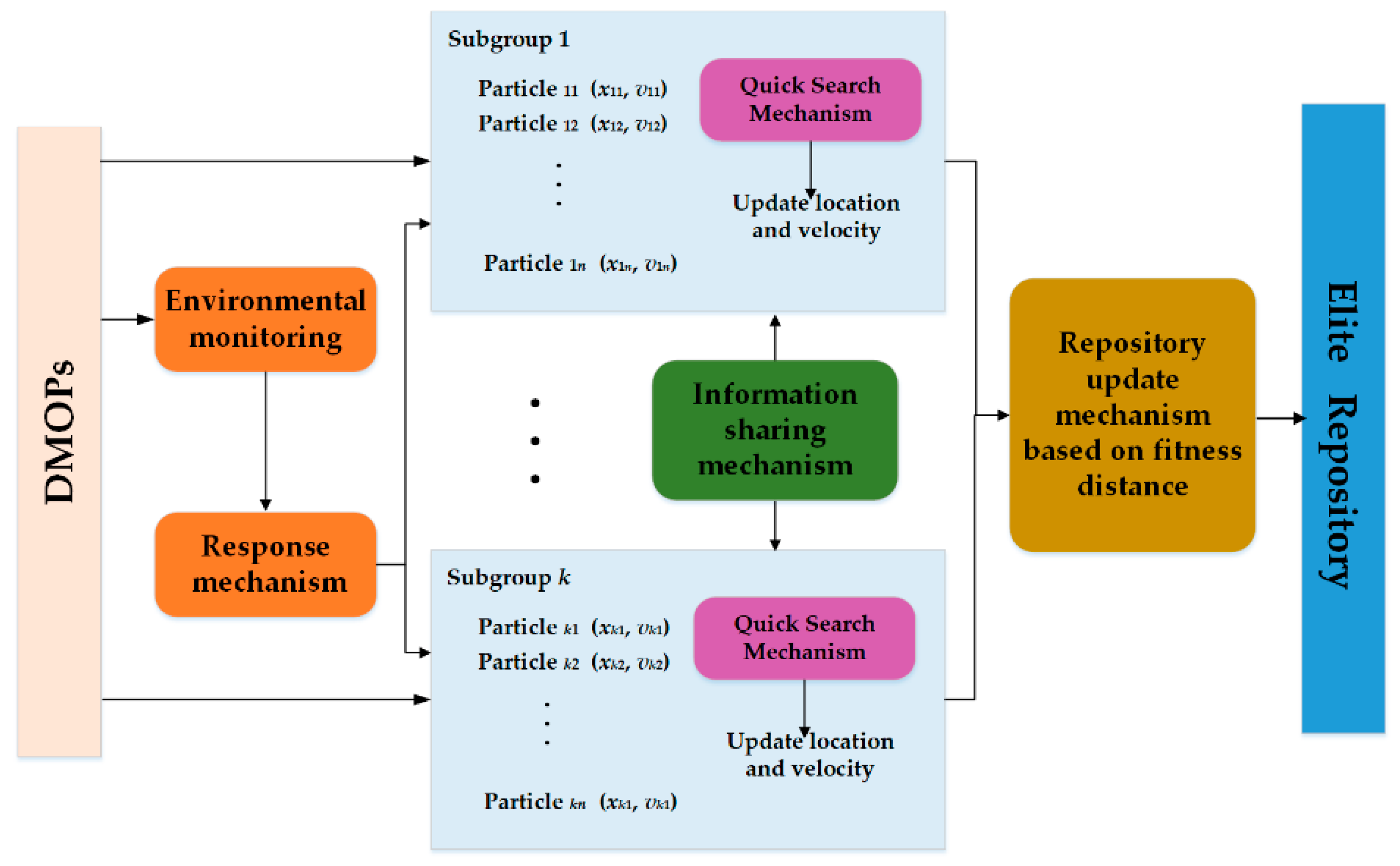
Figure 1 shows the composition of the DVEPSO/FD system, which overcomes the shortcomings of the DVEPSO method that cannot obtain a very accurate POF tracked after each objective changes. The repository update mechanism based on the fitness distance and quick search mechanism are designed to respond quickly when environmental changes are monitored.
The core structures of the DVEPSO/FD algorithm can be summarized as follows: information sharing mechanism, environmental monitoring and response mechanism, quick search mechanism, and repository update mechanism. A swarm of particles are used to solve DMOPs, and it is divided into subgroups. Each particle has its own location and velocity, which are updated in each iteration to obtain and . The information sharing mechanism is adapted to change information between subgroups. The system monitors changes in the environment in real time. Once it changes, the response mechanism will pick out part of the particles to make corresponding adjustments, and the quick search mechanism will be activated at the first time. The repository is used to store Pareto solutions and it is updated based on fitness distance to obtain an elite repository. The is picked up from the elite repository to better guide the particles.
Because the quality of the repository update mechanism largely determines whether the algorithm can filter out the good nondominant solutions, which will affect the accuracy of the POF found by the algorithm, an innovation is first made in the repository update mechanism. The repository update mechanism based on fitness distance is generally based on the crowding distance, which may delete the better solution, and is not conducive to the diversity of MOPSO. While the fitness distance is defined and introduced in DVEPSO/FD to streamline the repository, calculate the average of the distance between the nondominant solutions with respect to each fitness function, use its average characteristics to streamline the repository more than once, and eliminate nondominant solutions with invalid or poor performance. It could be more effective at guiding the selection of the global optimal solution, thus achieving a better choice of nondominant solutions and maintaining a more efficient repository.
In addition, in order to improve the efficiency of the algorithm and quickly find the POF, this paper proposed the addition of a quick search mechanism, that is, dynamically adjusting the flight parameters before and after the first change of the environment. Compared with the DVEPSO method, the repository update mechanism based on fitness distance could improve the distribution of nondominant solutions, and the quick search mechanism could adjust dynamically to improve the search speed.
3.2. Module Design
3.2.1. Repository Update Mechanism Based on Fitness Distance
In the past, the repository update mechanism was usually based on crowding distance, and the nondominant solution beyond the repository size was eliminated directly by calculating the crowding distance, while the fitness distance was used in DVEPSO/FD to streamline the repository. The definitions of the crowding distance and fitness distance are as follows.
Definition 1 ([25]). Crowding distance is defined in Equation (4). Suppose there are a total ofsub-objectives, and the initial crowding distance of all individuals is .
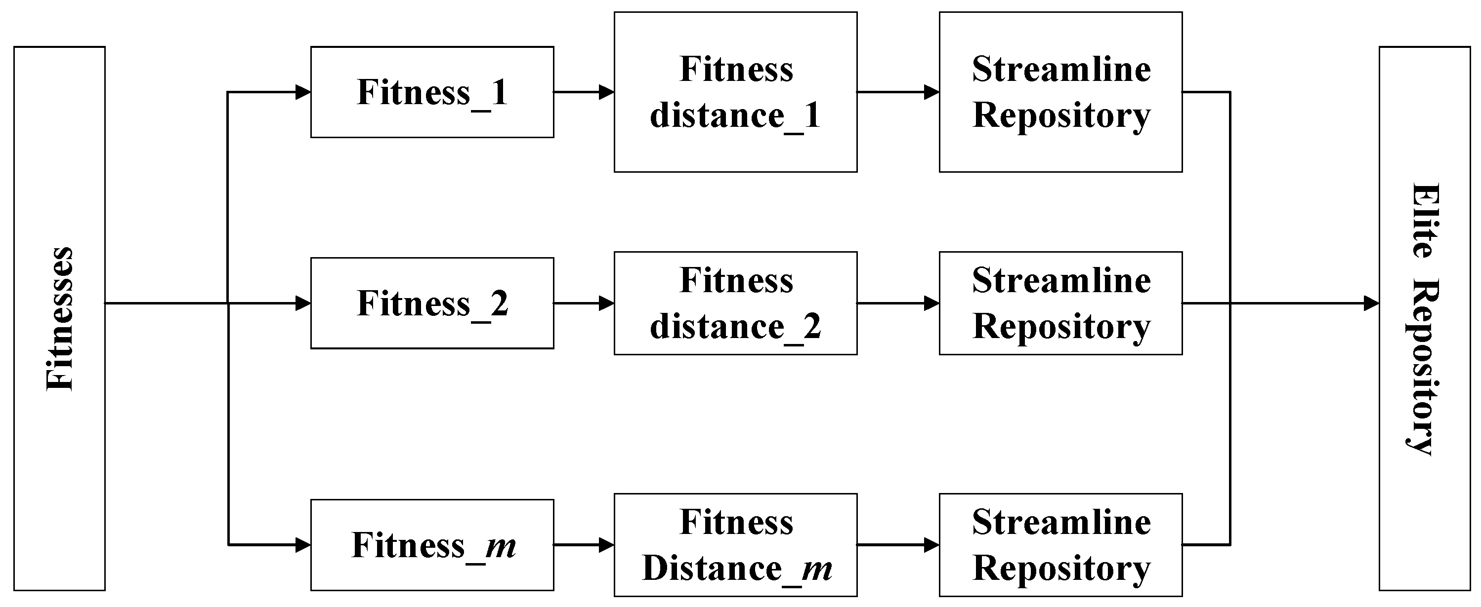
whereis the crowing distance of particleandis the number of fitness functions, where the fitness function is the specific function model of the each objective optimization problem.is the-th fitness function value of particle. Definition 2. The definition and equation of fitness distance is shown in Equation (5).whereis the fitness distance of the individualrelative to the objective, andis the fitness function value of the individualrelative to the objective. It is important to point out that if there areobjectives, then each particle has and totally hasfitness distances. Figure 2 shows a schematic diagram of the repository update mechanism based on fitness distance. The optimization problem could be divided into several independent fitness functions. For each fitness function, each particle can calculate a corresponding fitness distance. The fitness distance of the nondominant solution is calculated and compared with the set threshold
to determine whether the nondominant solution is retained or not. All of the fitness distances are used to streamline the repository independently. Compared to the crowding distance, the repository update mechanism based on the crowding distance is only streamlined once, but the one based on the fitness distance will be streamlined
times according to the number of fitness functions. The advantage of this design is that it can retain its optimal solution for each fitness function. Especially in the case of environmental changes, the response of each objective is different, so the changes of each fitness function are different. The repository update mechanism based on the crowding distance may miss the optimal solution, while the proposed method is more conducive to solve dynamic optimization problems.
After completing all the streamlining actions, the remaining nondominant solutions form the elite repository. The elite repository also has a certain capacity, so the number of nondominant solutions in the elite repository should also be limited, and the elimination rule is also based on crowding distance when out of range.
3.2.2. Quick Search Mechanism
The Pareto optimal frontier of the dynamic algorithm also changes according to the change in the objective function. The Pareto optimal frontier of the first generation is difficult to find. The Pareto optimal frontier of the offspring is changed on the basis of the previous generation, so it will be easier to find than the first generation.
In order to improve particles’ ability of finding the initial POF quickly in the early stage, the quick search mechanism is proposed. Iterations before the first time environmental change can be named the Quickly Search stage (QS stage); therefore, the value of , , and in the QS stage should be dynamically adjusted. After the QS stage, the next POFs are usually easily found on the basis of the existing data of the previous POF, and this stage can be named the Non-QS stage. The parameters do not need to be dynamically adjusted in the Non-QS stage, which does not contribute much to save the runtime.
For the adaptive PSO, the values of
and learning factor
are required to be large in the early iteration to enhance the search ability of the local optimal value. When close to the POF, the search ability of this local optimal value should be reduced, so the later value is small. Conversely, the value of learning factor
is required to change from small to large. In the later iteration, the influence of the global optimal value is enhanced to make more particles close to the POF. The specific adjustment equations of these three parameters in the QS stage are shown in (6)–(8).
where
, and
is the current number of iterations.
3.2.3. Other Structures
- (1)
Information sharing mechanism
Each particle has a local optimum and a global optimal to guide its search in the search space. The local optimum of a particle is its personal best,
, which is the best position where the particle is currently found. When there are no changes in the environment, the global guide of particles,
, is selected from one of the subgroups through a knowledge sharing mechanism. In this way, the
of each population may become
, that is, the information of its own population is transmitted through
, and then other populations are affected by
, thereby achieving information sharing between the populations [
21].
There are many mechanisms for information sharing, such as the circular loop strategy and roulette selection. Among them, the circular loop strategy is relatively simple. The selection method of subgroup
is shown in Equation (9).
- (2)
Environmental monitoring and response mechanism
After each iteration, randomly select some particles as sentinel particles, and evaluate the environment before the start of the next iteration. If the differences in the fitness values of the sentinel particles between current and previous are all greater than a certain value, the environment is considered changed. If a change in the environment is detected, the particles of the corresponding subgroup are reinitialized at a certain ratio, which is usually 30%.
3.3. The Pseudo-Code of the Algorithm
The repository update mechanism based on fitness distance possesses the elite repository to improve the distribution of nondominant solutions, and the quick search mechanism adjusts the flight parameters dynamically, so the DVEPSO/FD responds quickly when environmental changes are monitored. The pseudo-code of the DVEPSO/FD is shown in
Table 1.
5. Conclusions
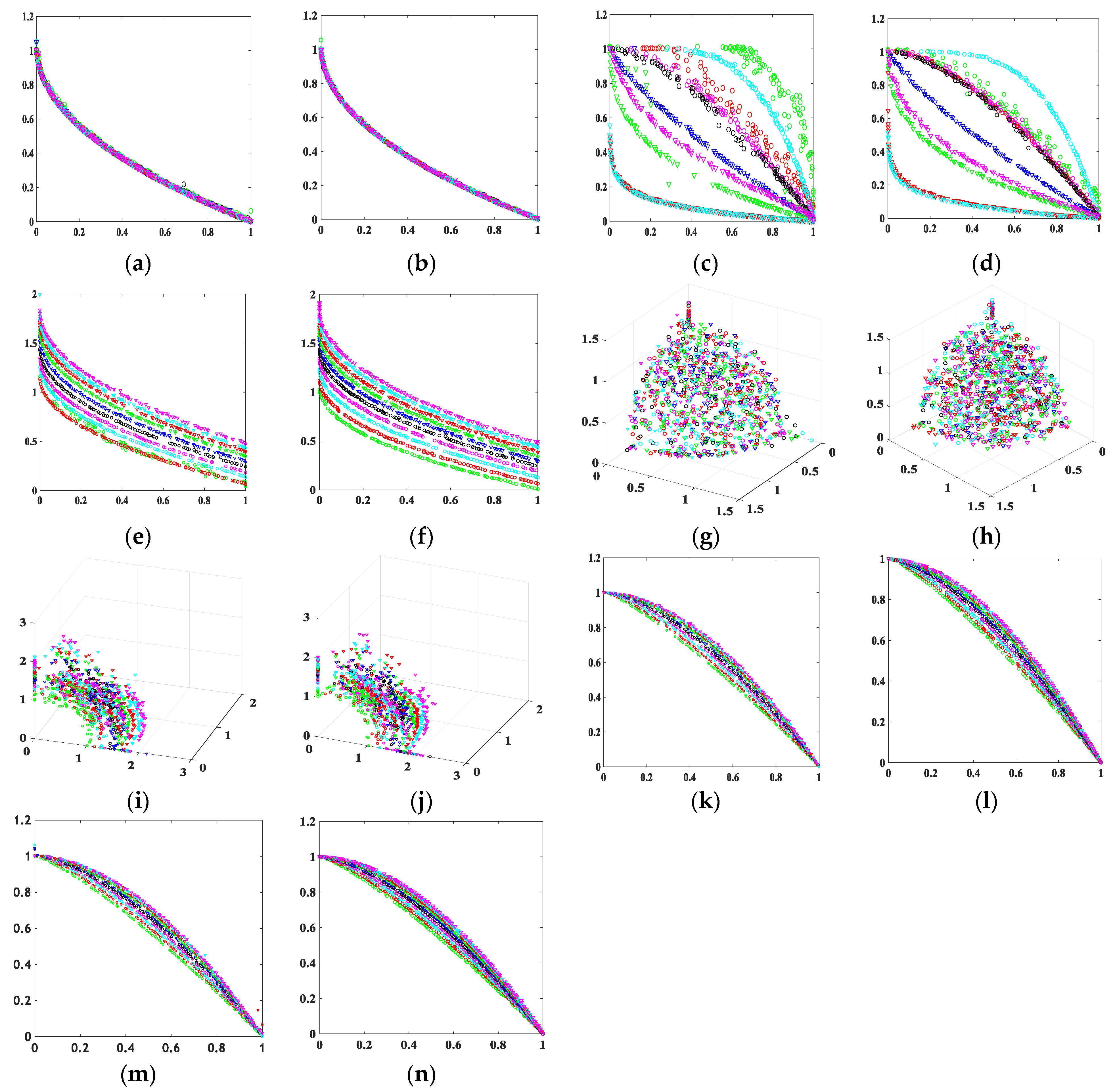
In this paper, a quick search dynamic vector-evaluated particle swarm optimization algorithm based on fitness distance (DVEPSO/FD) is proposed. Taking the DVEPSO method as a foundation, the repository update mechanism using the fitness distance and quick search mechanism are designed aiming for a good dynamic change adaptability and solving set ability of the dynamic multi-objective optimization problem. The fitness distance is used to streamline the repository to achieve better optimal solutions, and the flight parameters of the particles are adjusted dynamically to improve the search speed. Both from the figures generated by the experiments of test functions and the values of performance indexes, the DVEPSO/FD has a better accuracy of the POF than the basic DVEPSO, obtains a better POS, and maintains the same strong stability.
From the perspective of the overall algorithm structure, the update mechanism of the repository has a great influence on whether the optimal value could be found closer to the real POF or not. DVEPSO/FD verifies this more clearly by improving this mechanism. Of course, other structures of the algorithm are also important, such as the environmental monitoring and response mechanism and information sharing mechanism. They will influence whether the algorithm can respond quickly and accurately to changes in the environment and correctly grasp the general direction of all population evolutions. This is also the direction of the author’s future research.


