Blood Flow in Multi-Sinusoidal Curved Passages with Biomimetic Rheology: An Application of Blood Pumping

Abstract

The unsteady flow of biological liquid through non-uniform pumps under porosity impacts is considered. The Jeffrey fluid is used as blood in the current study, which is also characterized as viscoelastic fluid because of its dual characteristics: on the one hand, its viscosity in nature; on the other hand, its elastic effect. Rheological equations are framed in a curvilinear coordinates system, and porosity influences are simulated with the body force term in momentum equations. The flow system has been transformed from fixed to wave frame using a linear–mathematical transformation between these two frames. In the next mathematical steps, these transformed equations are given in non-dimensional form using physical variables. The system of PDE is reduced to an ODE under lubrication theory and long wavelength approximation. Solutions to reduced ordinary differential equations are obtained numerically in MATLAB software via a BVP4C scheme. The physical impacts of the involved parameters on flow features, such as curvature, porosity (Darcy’s number), non-uniformity, and viscoelastic parameters, have been visualized graphically. Multi-sinusoidal waves are used in the boundary wall of the curved pump for peristaltic pumping. The magnitude of velocity profile for a saw-tooth wave (trapezoidal wave) is larger (smaller) than all other natures of peristaltic waves. The larger intensity of Darcy’s number has a dynamic role in the reduction of peristaltic pumping, whereas the opposite behavior is noticed when increasing the non-uniform nature of a channel. A comparison between all multi-sinusoidal waves is also addressed. The results of the present research shall be very productive for the manufacture of peristaltic pumps for drug delivery and bio-medical systems.

1. Introduction

In bio-fluid mechanics, peristaltic pumping is an important transportation phenomenon due to the continuous expansion and contraction of the boundary walls of flexible vessels/tubes. Peristaltic pumping has played a dynamic role in numerous biological processes and has been simulated by researchers and scientists for the manufacture of nano-industrial instruments such as the small intestine, finger pumps, robotic pumps, and artificial heart-lung machines [1,2,3]. All of these pumps perform mechanically under the peristaltic mechanism. Many researchers have performed productive investigations in this domain after the remarkable work of Latham [4]. These investigations have also included both viscous and non-viscous liquids. Mathematical modeling related to peristaltic pumping was initially performed by Shapiro et al. [5]. Hayat et al. [6] studied the peristaltic transportation of Maxwell liquid under the creeping phenomena in a porous medium. Numerical simulations of viscoelastic liquid in a curved channel have been studied by Javid et al. [7], who used peristaltic waves at the boundary walls for pumping under creeping theory. The authors highlighted the impact of a larger Weissenberg number (viscoelastic parameter) on peristaltic pumping features. They highlighted a comparison between curved and straight channels. Recently, Abbasi et al. [8] performed a numerical formulation of hybrid liquid in the presence of an electric field due to peristalsis. The authors drew graphs of the various features using the shooting technique under creeping theory. They also compared the thermal efficiency of hybrid fluid with nanofluid. They noticed that the velocity profile is reduced under a larger magnetic strength. A similar effect was observed in a velocity profile by increasing the Helmholtz–Smoluchowski velocity. Abd-Alla and Abo-Dahab [9] studied the peristaltic motion of Jeffrey fluid through an asymmetrical channel. They also noticed physical impacts of the magnetic field and rotation on rheological characteristics under biological assumptions. The impact of the Hall parameter and the magnetic field on the motion of Jeffrey fluid in a non-uniform rectangular duct via peristaltic pumping under lubrication theory has been studied by Ellahi et al. [10]. The biomimetic propulsion of viscoelastic fluid in a non-uniform rectangular duct was studied by Bhatti et al. [11], who used the Jeffrey fluid model as a viscoelastic fluid in their flow analysis. Additionally, they also highlighted the impact of the magnetic field on various features related to peristaltic pumping under long wavelength assumption. A mathematical formulation related to the bio-rheological motion of viscoelastic liquid in an asymmetric nano-channel via peristaltic pumping has been studied by Tripathi et al. [12], who also used an electronic device (an axial electric field) to transport fluid under a low Reynold’s number approximation and Debye–Hückel linearization. Their results are productive for drug designed micro-chips. Numerical simulation related to the biomimetic rheology of viscoelastic liquid (blood) in a non-uniform channel was studied by Javid et al. [13], who noted that the magnetic field has a vigorous role in the enhancement of pumping phenomena. The electro-kinetic flow of bio-rheological fluid in a convergent channel via peristaltic pumping was studied by Javid et al. [14]. The authors observed the combined effects of porosity medium (Darcy’s number), magnetic field (Hartmann number), and electric field (electroosmosis parameter) on flow characteristics under long wavelength supposition. The peristaltic motion of couple stress fluid through a non-uniform channel under porosity effects has been discussed by Javid et al. [15], who noticed that the larger intensity of a porous medium has a remarkable role in the escalation of the magnitude of the velocity profile and the pressure gradient. Akram and Saleem [16] analyzed the flow of Carreau liquid in a rectangular duct via peristaltic transport under the creeping assumption. Additionally, the physical impact of heat transfer on biomimetic propulsion are also addressed. The authors used different waveforms of peristaltic pumping in their analysis. Akram et al. [17] debated the physical impacts of partial slip and lateral walls on the sinusoidal motion of a non-Newtonian fluid through a rectangular duct. The authors used different waveforms in their flow study under lubrication theory. They found exact solutions to rheological equations and highlighted the impact of embedded parameters on different peristaltic features through graphs. The numerical simulation of peristaltic motion in a curved channel was demonstrated by Javid et al. [18]. The physical impact of the magnetic field and the time relaxation parameter on the different flow features related to peristaltic pumping are discussed with the help of graphs in wave frame. The main aim of this study was to observe the physical behavior of flow features under a larger intensity of the magnetic field and viscoelastic parameter. The authors noted these effects for five different wave frames under a low Reynolds number assumption.

Motivated by the wider applications of blood rheology and peristaltic pumping in biomedical science, the current investigation looks at the physical influences of porosity parameters and different wave frames on the flow of a viscoelastic fluid in a non-uniform channel. The key purpose of the current formulation is to examine the influence of porous media on the peristaltic transportation of a viscoelastic liquid through non-uniform curved pumps. Additionally, five different types of peristaltic waves are used in the current investigation under lubrication theory. The mathematical modeling of the waves and their graphical analysis are given in the next two sections. The interesting findings and key conclusions of the current modeling are given in the last section.

2. Mathematical Modeling of Blood Pumping

Let us consider two-dimensional blood flow in a curved pump having the half-width $A$. The flow takes place due to the peristaltic propulsion under porosity effects. We have taken curvilinear coordinates $\left(\overline{\eta },\overline{\varsigma }\right)$ for the pump with $\overline{\eta }$, which represents the axial coordinate, and $\overline{\varsigma }$, which is the radial coordinate of the flow geometry (see Figure 1). 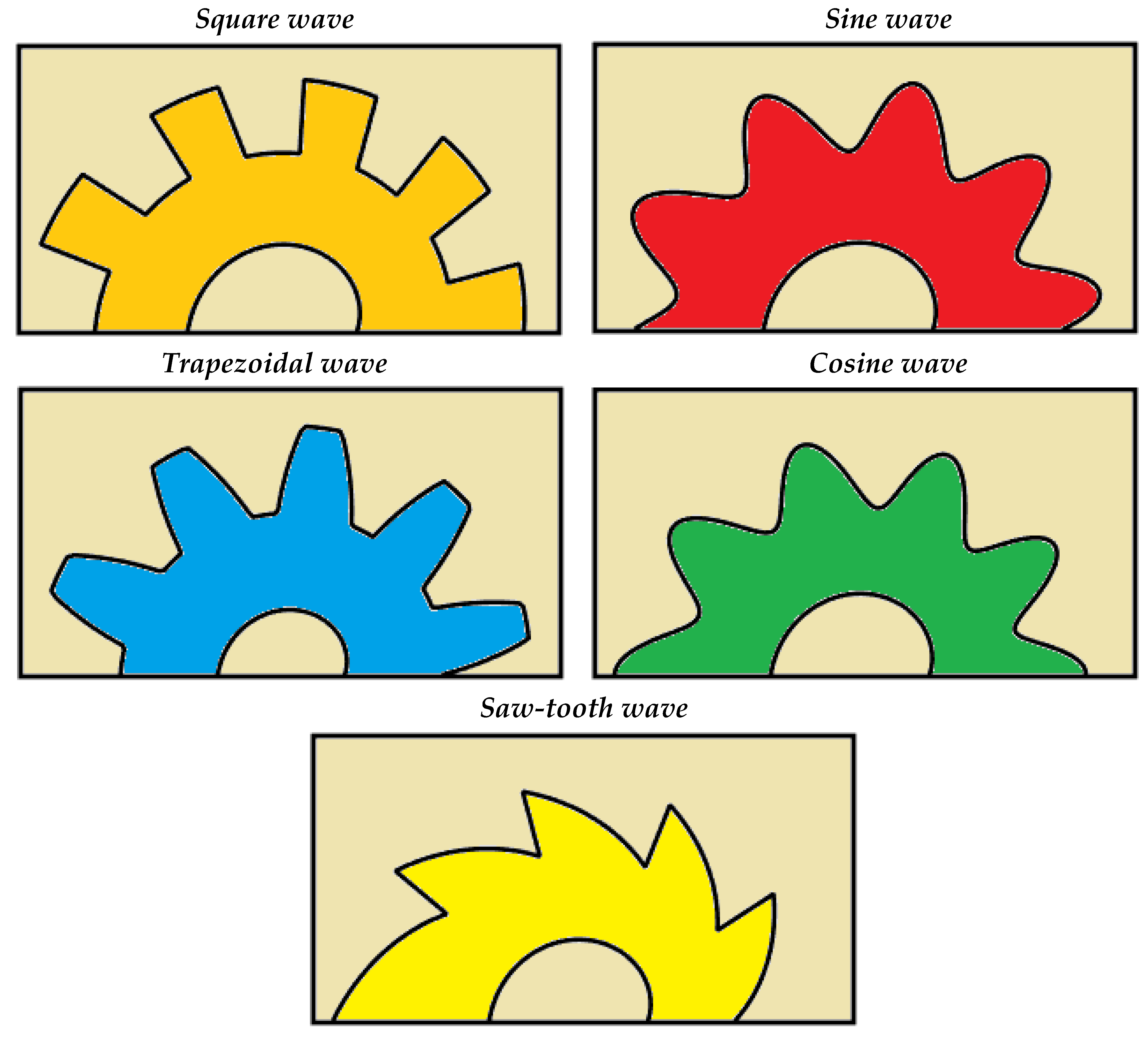Let ${\sigma }^{*}$ represent the radius of curvature and $\omega$ be the wave speed. In the current study, we have used multi-sinusoidal wave frames, such as a square wave, cosine wave, trapezoidal wave, sin wave, and sawtooth wave for blood propulsion. The rheological geometry is mathematically expressed as [18,19]:

$$-\overline{H}\left(\overline{\eta },\overline{t}\right)=-A-\overline{\alpha }\left(\frac{2\pi }{\mathsf{ϵ}}\left(\overline{\eta }-\varpi \overline{t}\right)\right),$$

(1)

Square wave

$$\overline{H}\left(\overline{\eta },\overline{t}\right)=B\left[\frac{4}{\pi }{{\displaystyle \sum }}_{j=1}^{\infty }\frac{{\left(-1\right)}^{j+1}}{\left(2j-1\right)}cos\left(\frac{2\pi }{\mathsf{ϵ}}\left(2j-1\right)\left(\overline{\eta }-\varpi \overline{t}\right)\right)\right]+A+\overline{\alpha }\left(\frac{2\pi }{\mathsf{ϵ}}\left(\overline{\eta }-\varpi \overline{t}\right)\right),$$

(2)

Sine wave

$$\overline{H}\left(\overline{\eta },\overline{t}\right)=Bsin\left(\frac{2\pi }{\mathsf{ϵ}}\left(\overline{\eta }-\varpi \overline{t}\right)\right)+A+\overline{\alpha }\left(\frac{2\pi }{\mathsf{ϵ}}\left(\overline{\eta }-\varpi \overline{t}\right)\right),$$

(3)

Trapezoidal wave

$$\overline{H}\left(\overline{\eta },\overline{t}\right)=B\left[\frac{32}{{\pi }^2}{{\displaystyle \sum }}_{j=1}^{\infty }\frac{sin\left(\frac{\pi }{8\mathsf{ϵ}}\left(2j-1\right)\right)}{{\left(2j-1\right)}^2}sin\left(\frac{2\pi }{\mathsf{ϵ}}\left(2j-1\right)\left(\overline{\eta }-\varpi \overline{t}\right)\right)\right]+A+\overline{\alpha }\left(\frac{2\pi }{\mathsf{ϵ}}\left(\overline{\eta }-\varpi \overline{t}\right)\right),$$

(4)

Cosine wave

$$\overline{H}\left(\overline{\eta },\overline{t}\right)=Bcos\left(\frac{2\pi }{\mathsf{ϵ}}\left(\overline{\eta }-\varpi \overline{t}\right)\right)+A+\overline{\alpha }\left(\frac{2\pi }{\mathsf{ϵ}}\left(\overline{\eta }-\varpi \overline{t}\right)\right),$$

(5)

Saw-tooth wave

$$\overline{H}\left(\overline{\eta },\overline{t}\right)=B\left[\frac{8}{{\pi }^3}{{\displaystyle \sum }}_{j=1}^{\infty }\frac{{\left(-1\right)}^{j+1}}{{\left(2j-1\right)}^2}sin\left(\frac{2\pi }{\mathsf{ϵ}}\left(2j-1\right)\left(\overline{\eta }-\varpi \overline{t}\right)\right)\right]+A+\overline{\alpha }\left(\frac{2\pi }{\mathsf{ϵ}}\left(\overline{\eta }-\varpi \overline{t}\right)\right),$$

(6)

where $-\overline{H}$ is the lower wall, $\overline{H}$ is the upper wall, $\mathsf{ϵ}$ is the wavelength, $B$ is the wave amplitude, $\overline{t}$ is the time, $\overline{\alpha }$ is the non-uniform parameter, and $\varpi$ is the wave speed.

The velocity field for the present rheological analysis is defined as $\left(\overline{V}\left(\overline{\eta },\overline{\varsigma },\overline{t}\right), \overline{W}\left(\overline{\eta },\overline{\varsigma },\overline{t}\right),0\right)$. Here, $\overline{V}\left(\overline{\eta },\overline{\varsigma },\overline{t}\right)$ and $\overline{W}\left(\overline{\eta },\overline{\varsigma },\overline{t}\right)$ represent the radial and axial components of the velocity field. Due to two-dimensional rheology, no velocity component exists in perpendicular direction to the $\overline{\eta }\overline{\varsigma }$–plane. Here, it is important to note that no external force is required to transport the liquid except the abovementioned peristaltic waves.

In the current investigation, the Jeffrey fluid model uses a blood liquid. The constitutive equation related to the viscoelastic model is defined as [20,21,22]:

$$\overline{\tau }=-p\overline{I}+\overline{\phi },$$

(7)

$$\overline{\phi }=\frac{\mu }{1+\beta }\left({\overline{\gamma }}_1+{\beta }^{*}\frac{D{\overline{\gamma }}_1}{D\overline{t}}\right),$$

(8)

where $\mu$ is the dynamic viscosity, $\left(\beta ,{\beta }^{*}\right)$ are the material variables of Jeffrey fluid, ${\overline{\gamma }}_1$ is the first Rivlin–Ericksen tensor, and $D/D\overline{t}$ is the material derivative.

The mathematical definitions of ${\overline{\gamma }}_1$ and $D/D\overline{t}$ are:

$${\overline{\gamma }}_1=grad\overline{U}+{\left(grad\overline{U}\right)}^T,$$

(9)

$$\frac{D}{D\overline{t}}=\frac{\partial }{\partial \overline{t}}+\overline{U}·\overline{\nabla },$$

(10)

where $\overline{U}$ is the velocity field, $\overline{\nabla }$ is the Nabla operator, and $T$ is the transpose.

The flow equations in terms of curvilinear coordinates dealing with the curved pumps are described as [23,24,25,26,27,28,29]:

$$\frac{\partial }{\partial \overline{\varsigma }}\left(\left({\sigma }^{*}+\overline{\varsigma }\right)\overline{W}\right)+{\sigma }^{*}\frac{\partial \overline{V}}{\partial \overline{\eta }}=0,$$

(11)

$$\begin{array}{c}\frac{\partial \overline{W}}{\partial \overline{t}}+\overline{W}\frac{\partial \overline{W}}{\partial \overline{\varsigma }}+\frac{\overline{V}\beta }{\overline{\varsigma }+{\sigma }^{*}}\frac{\partial \overline{W}}{\partial \overline{\eta }}-\frac{{\overline{V}}^2}{\overline{\varsigma }+{\sigma }^{*}}=-\frac{1}{\xi }\frac{\partial \overline{p}}{\partial \overline{\varsigma }}+\mathsf{{\rm Y}}(\frac{1}{\overline{\varsigma }+{\sigma }^{*}}\frac{\partial }{\partial \overline{\varsigma }}\left(\left(\overline{\varsigma }+{\sigma }^{*}\right){\overline{\zeta }}_{\overline{\varsigma }\overline{\varsigma }}\right)+\hfill \\ \hspace{1em}\left(\frac{{\sigma }^{*}}{\overline{\varsigma }+{\sigma }^{*}}\right)\frac{\partial {\overline{\zeta }}_{\overline{\varsigma }\overline{\eta }}}{\partial \overline{\eta }}-\frac{{\overline{\zeta }}_{\overline{\eta }\overline{\eta }}}{\overline{\varsigma }+{\sigma }^{*}})-{\left(\frac{{\sigma }^{*}}{\overline{\varsigma }+{\sigma }^{*}}\right)}^2\frac{\mu \overline{V}}{{\mathsf{\kappa }}^2},\hfill \end{array}$$

(12)

$$\begin{array}{c}\frac{\partial \overline{V}}{\partial \overline{t}}+\overline{W}\frac{\partial \overline{V}}{\partial \overline{\varsigma }}+\frac{\overline{V}{\sigma }^{*}}{\overline{\varsigma }+{\sigma }^{*}}\frac{\partial \overline{V}}{\partial \overline{\eta }}+\frac{\overline{V}\overline{W}}{\overline{\varsigma }+{\sigma }^{*}}=-\frac{1}{\xi }\frac{{\sigma }^{*}}{\left(\overline{\varsigma }+{\sigma }^{*}\right)}\frac{\partial \overline{p}}{\partial \overline{\eta }}+\mathsf{{\rm Y}}(\frac{1}{{\left(\overline{\varsigma }+{\sigma }^{*}\right)}^2}\frac{\partial }{\partial \overline{\varsigma }}\left({\left(\overline{\varsigma }+{\sigma }^{*}\right)}^2{\overline{\zeta }}_{\overline{\varsigma }\overline{\eta }}\right)\hfill \\ +\left(\frac{{\sigma }^{*}}{\overline{\varsigma }+{\sigma }^{*}}\right)\frac{\partial {\overline{\zeta }}_{\overline{\eta }\overline{\eta }}}{\partial \overline{\eta }})-{\left(\frac{{\sigma }^{*}}{\overline{\varsigma }+{\sigma }^{*}}\right)}^2\frac{\mu \overline{W}}{{\mathsf{\kappa }}^2},\hfill \end{array}$$

(13)

where $\xi$ is the fluid density, $\overline{p}$ is the pressure, ${\overline{\zeta }}_{\overline{\varsigma }\overline{\varsigma }}, {\overline{\zeta }}_{\overline{\varsigma }\overline{\eta }}, {\overline{\zeta }}_{\overline{\eta }\overline{\eta }}$ are the extra stress tensor components, $\mathsf{\kappa }$ is the porosity parameter, and $\mathsf{{\rm Y}}=\mu /\xi$ is the kinematic viscosity.

The rheological system that is defined in Equations (11)–(13) deals with the unsteady state (the state in all rheological features strongly depends upon the time) using curvilinear coordinates. In order to shift this rheological system from an unsteady to a steady state, we use the following transformations:

$${\eta }^{\prime }=\overline{\eta }-\varpi \overline{t}, {\varsigma }^{\prime }=\overline{\varsigma }, v^{\prime }=\overline{V}, w^{\prime }=\overline{W}-\varpi , p^{\prime }=\overline{p}.$$

(14)

The transformed system of governing equations is given as:

$$\frac{\partial }{\partial {\varsigma }^{\prime }}\left(\left({\sigma }^{*}+{\varsigma }^{\prime }\right)\left(w^{\prime }+\varpi \right)\right)+{\sigma }^{*}\frac{\partial v^{\prime }}{\partial {\eta }^{\prime }}=0,$$

(15)

$$\begin{array}{c}-\varpi \frac{\partial w^{\prime }}{\partial {\eta }^{\prime }}+\left(w^{\prime }+\varpi \right)\frac{\partial w^{\prime }}{\partial {\varsigma }^{\prime }}+\frac{v^{\prime }\beta }{{\varsigma }^{\prime }+{\sigma }^{*}}\frac{\partial w^{\prime }}{\partial {\eta }^{\prime }}-\frac{{v^{\prime }}^2}{{\varsigma }^{\prime }+{\sigma }^{*}}=-\frac{1}{\xi }\frac{\partial p^{\prime }}{\partial {\varsigma }^{\prime }}+\mathsf{{\rm Y}}(\frac{1}{{\varsigma }^{\prime }+{\sigma }^{*}}\frac{\partial }{\partial {\varsigma }^{\prime }}\left(\left({\varsigma }^{\prime }+{\sigma }^{*}\right){\overline{\zeta }}_{{\varsigma }^{\prime }{\varsigma }^{\prime }}\right)+\hfill \\ \left(\frac{{\sigma }^{*}}{{\varsigma }^{\prime }+{\sigma }^{*}}\right)\frac{\partial {\overline{\zeta }}_{{\varsigma }^{\prime }{\eta }^{\prime }}}{\partial {\eta }^{\prime }}-\frac{{\overline{\zeta }}_{{\eta }^{\prime }{\eta }^{\prime }}}{{\varsigma }^{\prime }+{\sigma }^{*}})-{\left(\frac{{\sigma }^{*}}{{\varsigma }^{\prime }+{\sigma }^{*}}\right)}^2\frac{\mu v^{\prime }}{{\mathsf{\kappa }}^2},\hfill \end{array}$$

(16)

$$\begin{array}{c}--\varpi \frac{\partial v^{\prime }}{\partial {\eta }^{\prime }}+\left(w^{\prime }+\varpi \right)\frac{\partial v^{\prime }}{\partial {\varsigma }^{\prime }}+\frac{v^{\prime }{\sigma }^{*}}{{\varsigma }^{\prime }+{\sigma }^{*}}\frac{\partial v^{\prime }}{\partial {\eta }^{\prime }}+\frac{v^{\prime }\left(w^{\prime }+\varpi \right)}{{\varsigma }^{\prime }+{\sigma }^{*}}=-\frac{1}{\xi }\frac{{\sigma }^{*}}{\left({\varsigma }^{\prime }+{\sigma }^{*}\right)}\frac{\partial p^{\prime }}{\partial {\eta }^{\prime }}+\mathsf{{\rm Y}}(\frac{1}{{\left({\varsigma }^{\prime }+{\sigma }^{*}\right)}^2}\times \hfill \\ \frac{\partial }{\partial {\varsigma }^{\prime }}\left({\left({\varsigma }^{\prime }+{\sigma }^{*}\right)}^2{\overline{\zeta }}_{{\varsigma }^{\prime }{\eta }^{\prime }}\right)+\left(\frac{{\sigma }^{*}}{{\varsigma }^{\prime }+{\sigma }^{*}}\right)\frac{\partial {\overline{\zeta }}_{{\eta }^{\prime }{\eta }^{\prime }}}{\partial {\eta }^{\prime }})-{\left(\frac{{\sigma }^{*}}{{\varsigma }^{\prime }+{\sigma }^{*}}\right)}^2\frac{\mu \left(w^{\prime }+\varpi \right)}{{\mathsf{\kappa }}^2}.\hfill \end{array}$$

(17)

This rheological system is difficult to handle directly. In order to overcome this deficiency, researchers have introduced the scaling of physical variables. The key advantage of these variables is to reduce the rheological equations from partial to ordinary DEQs.

We now introduce the following scaling transformation: $\varsigma ={\varsigma }^{\prime }/A$ is the radial component, $\eta =2\pi /\mathsf{ϵ}{\eta }^{\prime }$ is the axial component, $v=v^{\prime }/\varpi$ is the radial velocity, $w=w^{\prime }/\varpi$ is the axial velocity, $Re=\xi \varpi A/\mu$ is the Reynold’s number, $p=2\pi A/\mathsf{ϵ}\varpi \mu$ is the pressure, $\delta =2\pi A/\mathsf{ϵ}$ is the delta (the wavelength ratio), $\sigma ={\sigma }^{*}/A$ is the radius of curvature, $\zeta =A/\varpi \mu \overline{\zeta }$ is the extra-stress tensor, $h=\overline{H}/A$ is the boundary wall, $\varphi =B/A$ is the wave-amplitude ratio, $\alpha =2\pi \overline{\alpha }/\mathsf{ϵ}$ is the non-uniform (divergent) parameter, and $DA=\mathsf{\kappa }/A^2$ is the Darcy’s number (porosity parameter).

The velocity components can also be stated in forms of stream function $\left(\psi \right)$, which are defined as:

$$v=\delta \frac{\sigma }{\varsigma +\sigma } \frac{\partial \psi }{\partial \eta },\hspace{1em}\hspace{1em}w=-\frac{\partial \psi }{\partial \varsigma }.$$

(18)

After using these dimensionless variables, we apply the lubrication theory and long wavelength approximations to obtain the reduced form of the rheological equations as:

$$\frac{dp}{d\varsigma }=0,$$

(19)

$$-\frac{\partial p}{\partial \eta }+\frac{1}{\sigma \left(\sigma +\varsigma \right)}\frac{\partial }{\partial \varsigma }\left({\left(\sigma +\varsigma \right)}^2{\tau }_{\eta \varsigma }\right)-\frac{1}{DA}\frac{{\sigma }^2}{\sigma +\varsigma }\left(1-\frac{d\psi }{d\varsigma }\right)=0.$$

(20)

Another form of Equation (20) is obtained using cross derivatives among these equations as:

$$\frac{\partial }{\partial \varsigma }\left(\frac{1}{\sigma \left(\sigma +\varsigma \right)}\frac{\partial }{\partial \varsigma }\left({\left(\sigma +\varsigma \right)}^2{\tau }_{\eta \varsigma }\right)\right)-\frac{{\sigma }^2}{DA}\frac{\partial }{\partial \varsigma }\left(\frac{1}{\sigma +\varsigma }\left(1-\frac{d\psi }{d\varsigma }\right)\right)=0.$$

(21)

where

$${\tau }_{\eta \varsigma }=\frac{1}{1+\beta }\left(-\frac{d^2\psi }{d{\varsigma }^2}-\frac{1}{\sigma +\varsigma }\left(1-\frac{d\psi }{d\varsigma }\right)\right),$$

(22)

where $\beta$ is the time relaxation (viscoelastic) parameter.

Substituting Equation (18) into Equation (21), we obtain

$$\frac{1}{1+\beta }\frac{\partial }{\partial \varsigma }\left(\frac{1}{\sigma \left(\sigma +\varsigma \right)}\frac{\partial }{\partial \varsigma }\left({\left(\sigma +\varsigma \right)}^2\left(-\frac{d^2\psi }{d{\varsigma }^2}-\frac{1}{\sigma +\varsigma }\left(1-\frac{d\psi }{d\varsigma }\right)\right)\right)\right)-\frac{1}{D{A}^2}\frac{\partial }{\partial \varsigma }\left(\frac{{\sigma }^2}{\sigma +\varsigma }\left(1-\frac{d\psi }{d\varsigma }\right)\right)=0.$$

(23)

The boundary conditions (BCs) in terms of stream function are defined below [7,23]:

$$\psi =-\frac{q}{2}, \frac{\partial \psi }{\partial \varsigma }=1 \mathrm{at} \varsigma =h,$$

(24)

$$\psi =\frac{q}{2}, \frac{\partial \psi }{\partial \varsigma }=1 \mathrm{at} \varsigma =-h,$$

(25)

where “q” is the time-average flow rate.

The mathematical equations of the multi-sinusoidal walls in the wave frame become:

$$-h\left(\eta \right)=-1-\alpha \left(\eta \right),$$

(26)

Square wave

$$h\left(\eta \right)=\varphi \left[\frac{4}{\pi }{{\displaystyle \sum }}_{j=1}^{\infty }\frac{{\left(-1\right)}^{j+1}}{\left(2j-1\right)}cos\left(\left(2j-1\right)\eta \right)\right]+1+\alpha \left(\eta \right),$$

(27)

Sine wave

$$h\left(\eta \right)=\varphi sin\left(\eta \right)+1+\alpha \left(\eta \right),$$

(28)

Trapezoidal wave

$$h\left(\eta \right)=\varphi \left[\frac{32}{{\pi }^2}{{\displaystyle \sum }}_{j=1}^{\infty }\frac{sin\left(\frac{\pi }{8\mathsf{ϵ}}\left(2j-1\right)\right)}{{\left(2j-1\right)}^2}sin\left(\left(2j-1\right)\eta \right)\right]+1+\alpha \left(\eta \right),$$

(29)

Cosine wave

$$h\left(\eta \right)=\varphi cos\left(\eta \right)+1+\alpha \left(\eta \right),$$

(30)

Saw-tooth wave

$$\left(\eta \right)=\varphi \left[\frac{8}{{\pi }^3}{{\displaystyle \sum }}_{j=1}^{\infty }\frac{{\left(-1\right)}^{j+1}}{{\left(2j-1\right)}^2}sin\left(\left(2j-1\right)\left(\overline{\eta }-\varpi \overline{t}\right)\right)\right]+1+\alpha \left(\eta \right).$$

(31)

Due to the complex nature of the differential equation, its exact solution is hard to find. However, in the current analysis, we are interested in the numerical results of flow equations using the BVP4C method in the MATLAB program.

The mathematical term $\partial p/\partial \eta$ represents the partial derivative of pressure $\left(p\right)$ with respect to the axial coordinate $\left(\eta \right)$. Its numerical integration from 0 to 2π yields the pressure-rise per wavelength:

$$\Delta p={{\displaystyle \int }}_0^{2\pi }\frac{dp}{d\eta }d\eta .$$

(32)

Procedure of BVP4C Numerical Technique: The BVP4C technique based upon a collocation method for finding the numerical solution of BVP of the special form

$$F^{\prime }=s\left(x,F,\mathit{o}\right),\hspace{1em}\hspace{1em}\hspace{1em}\hspace{1em}a1\le x\le a2$$

(33)

Concerned with nonlinear two-point BCs,

$$\chi \left(F\left(a1\right),F\left(a2\right),\mathit{o}\right)=\mathbf{0}.$$

(34)

where $\mathit{o}$ represents embedded parameters in the vector-form. For simplification, the governing equations and boundary conditions (BCs) are transformed into a linear system using the following rules:

Firstly, transform the whole flow system from a higher order to a first-order ODE. Secondly, a similar procedure is adopted to transform the higher order BCs to first-order BCs. The initial guess used should satisfy the BCs (or the Newtonian solution for the current problem). The main advantage in using this technique is that it is a very accurate method as compared with the shooting method, because sometimes the shooting method is unstable at initial points. The entire above procedure is created using MATLAB software. MATLAB is a programming language that deals with the multi-paradigm function/programming language. This language deals with all physical models in mathematical frameworks by developing a numeric computing environment. This mathematical tool is also productive to plot, analyze, and manipulate any numerical data and function. To obtain more information about the BVP4C technique, we direct readers to the research paper given in references [26,27].

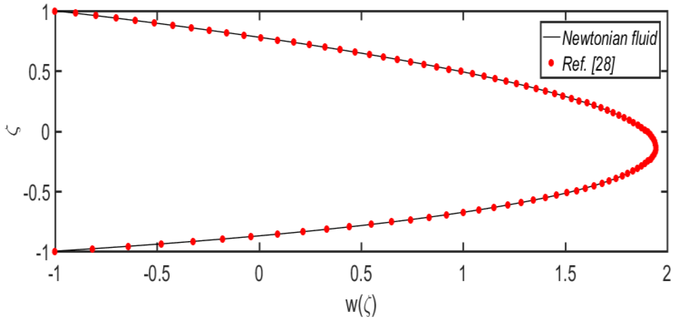
Figure 2 is plotted for the comparison of the numerical result with the analytical solution of viscous fluid given by Ali et al. [28]. This graph clearly validates the authenticity and accuracy of our numerical results. This figure is plotted using the following substitutions: $\alpha =\beta =0$ and $DA\to \infty$.

3. Physical Interpretation of Outcomes

The key purpose of this section is to scrutinize the physical impacts of embedded parameters such as the curvature parameter, the time relaxation (viscoelastic) parameter, the non-uniform parameter, and Darcy’s number (porosity) on the pressure gradient, peristaltic pumping, axial velocity, and streamline. The graphical results related to the pressure gradient, peristaltic pumping, axial velocity, and streamline are plotted with the MATLAB program. These results are shown in Figure 3, Figure 4, Figure 5, Figure 6 and Figure 7. The flow is observed under the multi-sinusoidal wave effects.

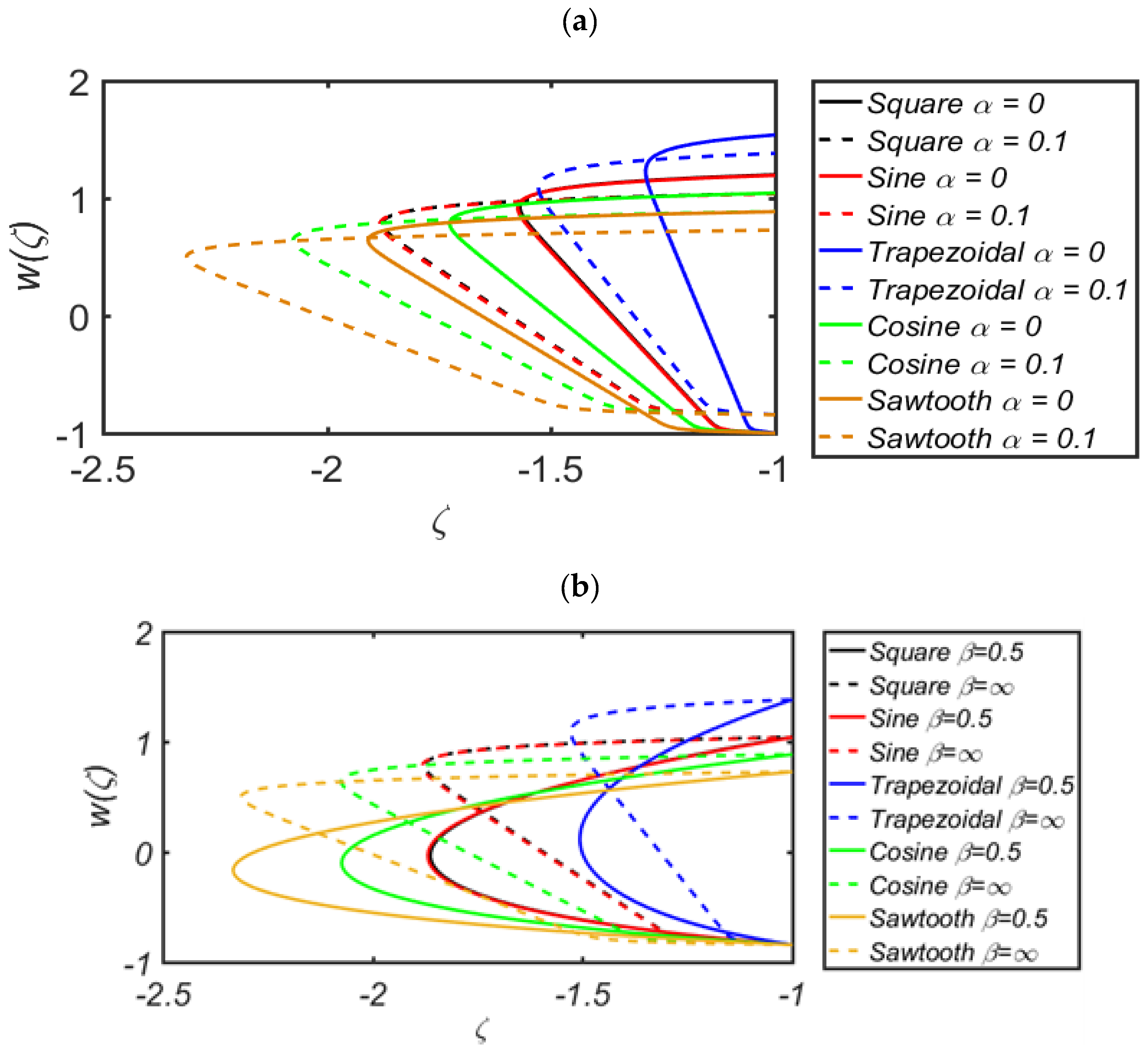
Figure 3a–d presents the physical behavior of the axial velocity versus the radial parameter with variation in the curvature parameter $\left(\sigma \right)$, time relaxation parameter $\left(\beta \right)$, non-uniform parameter $\left(\alpha \right)$, and Darcy’s number $\left(DA\right)$, respectively. We have plotted these graphs for multi-sinusoidal waves. Figure 3a is plotted for the physical impacts of the curvature parameter on the axial velocity $\left(w\left(\varsigma \right)\right)$ under larger porosity effects at the cross-sectional area $q=-3$. This figure shows that the magnitude of $w\left(\varsigma \right)$ decreases when increasing the numeric value of the curvature parameter from 1.5 to $\infty$. The asymmetric in $w\left(\varsigma \right)$ is observed for the curved channel at $\sigma =1.5$, and symmetry is observed for a straight channel at $\sigma \to \infty$. Sharp changes (boundary layers, BL) are predicted in the velocity profile due to the larger effects of a porous medium. Figure 3b shows that, by increasing the time relaxation parameter from 0.5 to $\infty$, the $w\left(\varsigma \right)$ shifts from the lower to the upper half. This figure is plotted under porosity and curvature effects. According to a literature survey, $w\left(\varsigma \right)$ shifts toward the upper half, and BL is predicted near the boundary walls for a larger strength of the viscoelastic parameter, e.g., $\beta =\infty$. The asymmetric in $w\left(\varsigma \right)$ is observed due to curvature effects. Another important element is the parabolic shape in $w\left(\varsigma \right), \mathrm{which}$ is noted for a smaller strength of the viscoelastic parameter, e.g., $\beta =0.5$. 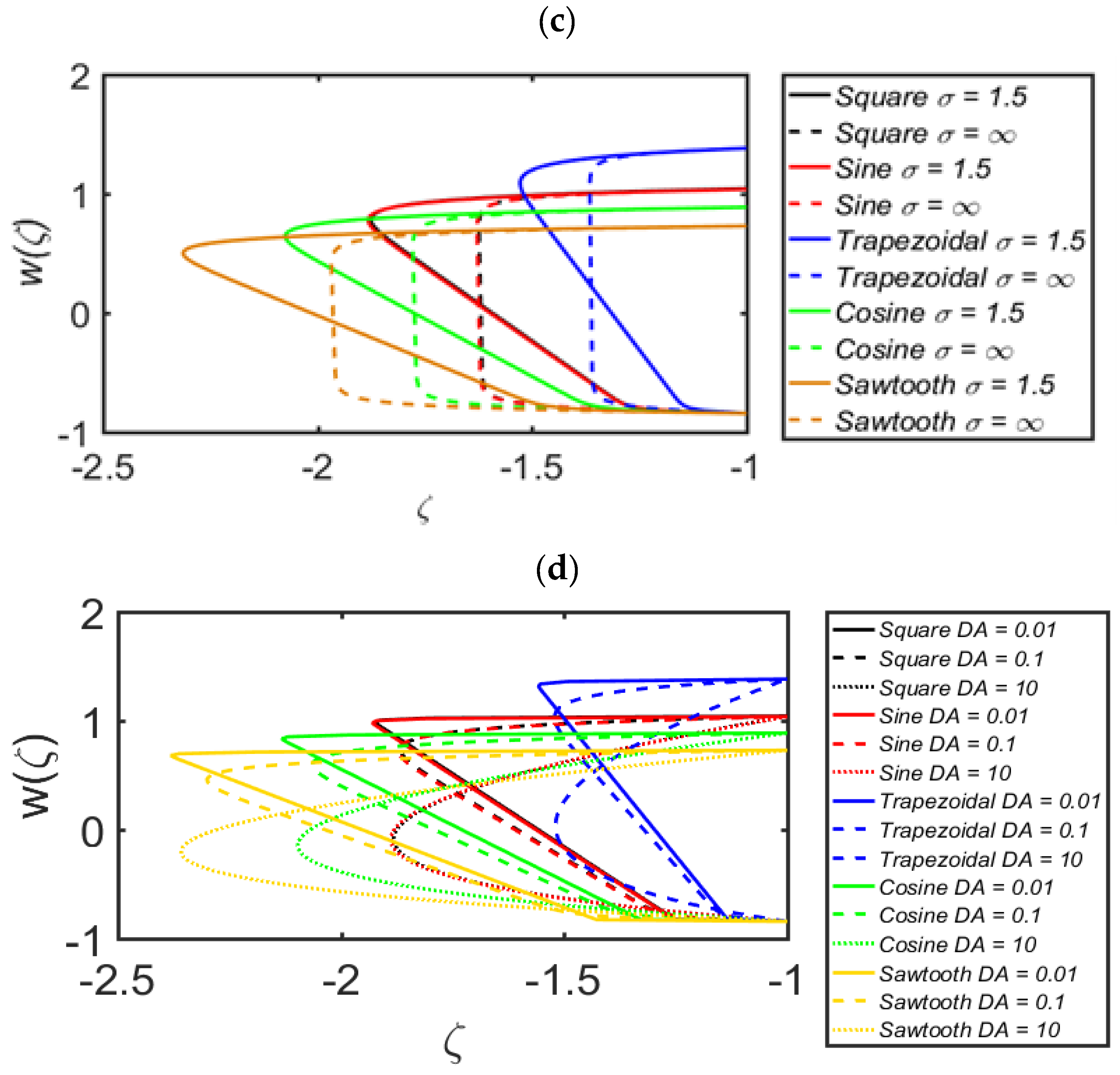The physical impacts of a non-uniform parameter on $w\left(\varsigma \right)$ are displayed in Figure 3c. This figure shows that, by increasing the numeric value of the non-uniform parameter from 0 to 0.1, $w\left(\varsigma \right)$ increases significantly. This figure is plotted under the combined effects of porosity medium and viscoelasticity. Physically, these results show that the non-uniform parameter has a remarkable role in enhancing the magnitude of $w\left(\varsigma \right)$. A similar pattern in the magnitude of $w\left(\varsigma \right)$ is observed in all multi-sinusoidal wave-frames. The magnitude of $w\left(\varsigma \right)$ does not increase or shift from the lower to the upper half with greater porosity effects, as shown in Figure 3d. Furthermore, the larger strength of the porosity effects has a vigorous effect to develop a BL pattern in $w\left(\varsigma \right)$ for all multi-sinusoidal wave frames. Additionally, it can be seen that the parabolic nature of the velocity profile is strongly affected under the larger strength of a porous medium. In all the above figures, it is predicted that the sawtooth wave has a larger magnitude of $w\left(\varsigma \right)$ as compared with all other waveforms (square wave, sine wave, trapezoidal wave, and cosine wave). A smaller magnitude of $w\left(\varsigma \right)$ is observed for the trapezoidal wave.

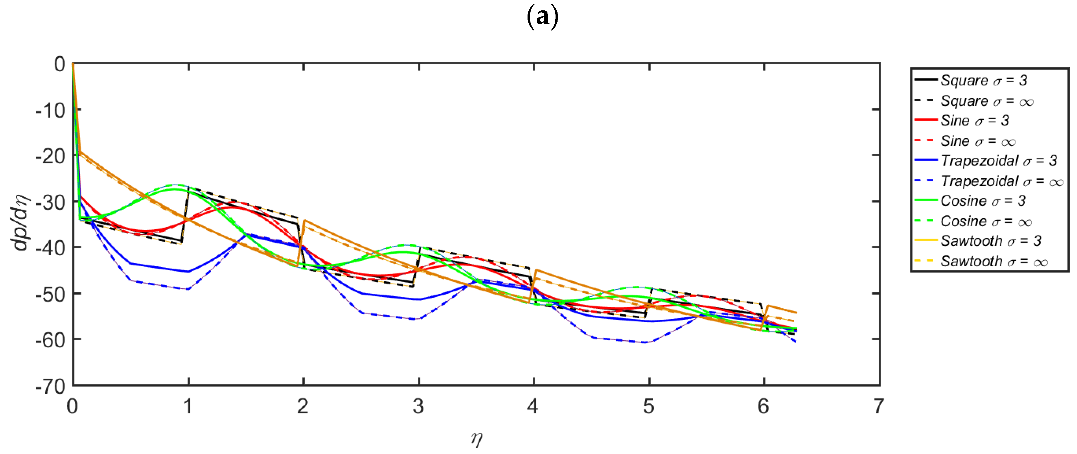
Figure 4a–d presents the physical behavior of the pressure gradient $\left(dp/d\eta \right)$ versus the axial parameter with a variation in the curvature parameter $\left(\sigma \right)$, time relaxation parameter $\left(\beta \right)$, non-uniform parameter $\left(\alpha \right)$, and Darcy’s number $\left(DA\right)$, respectively. We have plotted these graphs for multi-sinusoidal waves. Figure 4a is plotted for physical influences of the curvature parameter on $dp/d\eta$ under larger porosity effects at the cross-sectional area $q=-1.5$. This figure shows that the magnitude of $dp/d\eta$ increases with an increasing numerical value of the curvature parameter from 1.5 to $\infty$. The smooth lines represent the graph of a curved pump, and the dotted lines symbolize a straight pump. 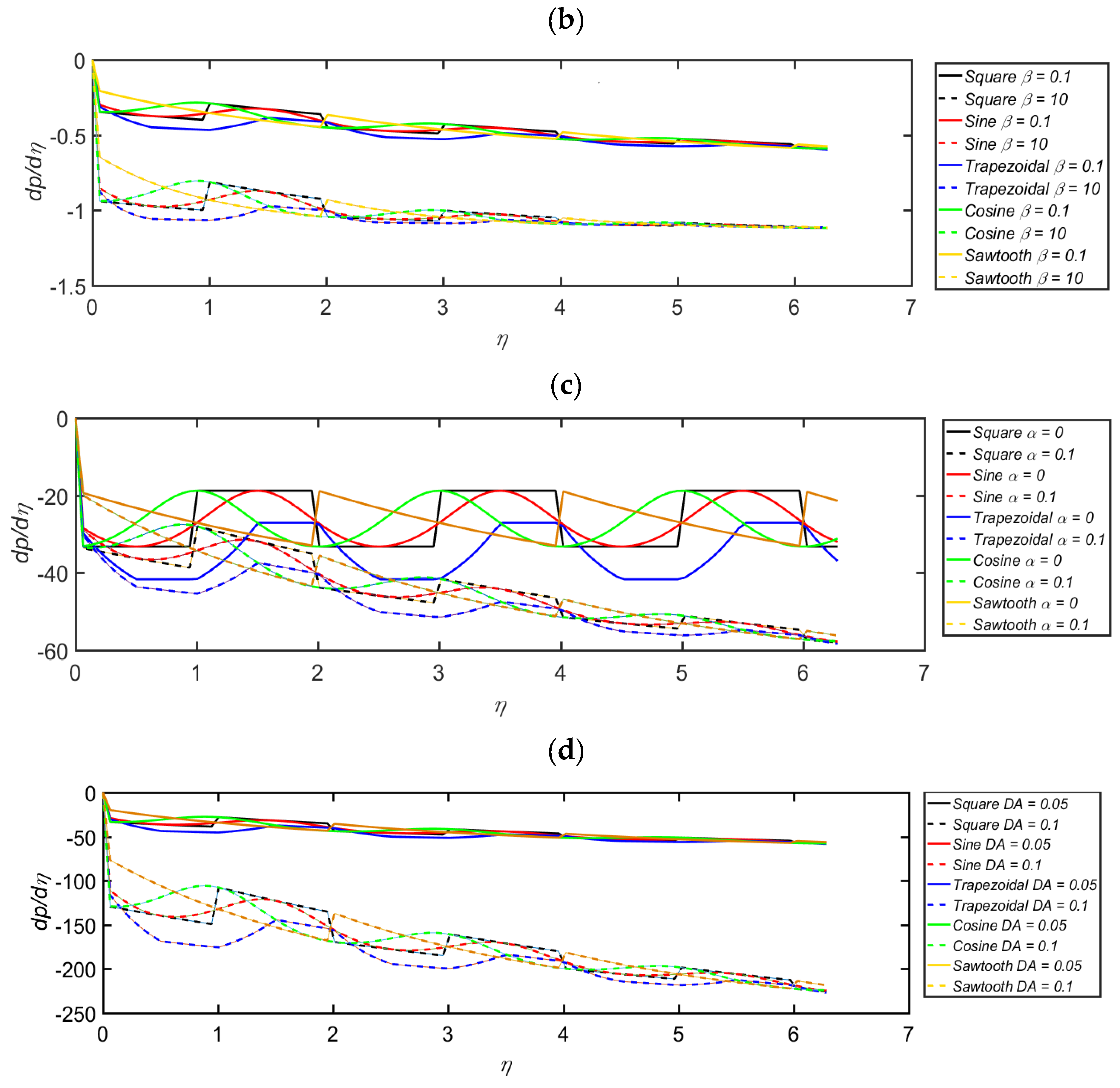Figure 4b illustrates that, by increasing the time relaxation parameter from 0.5 to $\infty$, the magnitude of $dp/d\eta$ is enhanced. This figure is plotted under porosity and curvature effects. This diagram is plotted for multi-sinusoidal wave frames. A similar nature of behavior is predicted in all these wave frames. The graphical effects of a non-uniform parameter on $dp/d\eta$ are displayed in Figure 4c. This figure reveals that, with an increasing numerical value of the non-uniform parameter from 0 to 0.1, $dp/d\eta$ increases significantly. This figure is plotted under the combined effects of porosity medium and viscoelasticity. Physically, these results show that the non-uniform parameter has a remarkable role in enhancing the magnitude of $dp/d\eta$. A similar pattern in the magnitude of $dp/d\eta$ is observed in all multi-sinusoidal wave frames. The magnitude of $dp/d\eta$ decreases with greater porosity effects, as shown in Figure 4d. Additionally, it can be seen that the wave nature of the pressure gradient is strongly affected under the larger strength of a porous medium. In all the above figures, it is predicted that the saw-tooth wave has a smaller magnitude of the pressure gradient as compared with all other waveforms (square wave, sine wave, trapezoidal wave, and cosine wave), and the largest magnitude of the pressure gradient is observed for the trapezoidal wave.

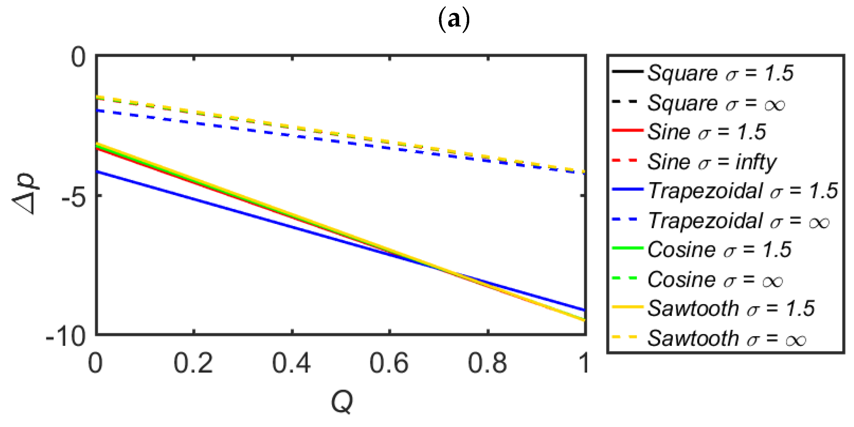
Figure 5a–d presents the physical behavior of pressure rise versus dimensionless flow rate with variation in curvature parameter $\left(\sigma \right)$, time relaxation parameter $\left(\beta \right)$, non-uniform parameter $\left(\alpha \right)$, and Darcy’s number $\left(DA\right)$, respectively. We have plotted these graphs for multi-sinusoidal waves. Figure 5a is plotted for the physical impact of the curvature parameter on the pressure rise under larger porosity effects. This figure shows that the magnitude of the pressure rise decreases with an increase in the numeric value of the curvature parameter from 1.5 to $\infty$. 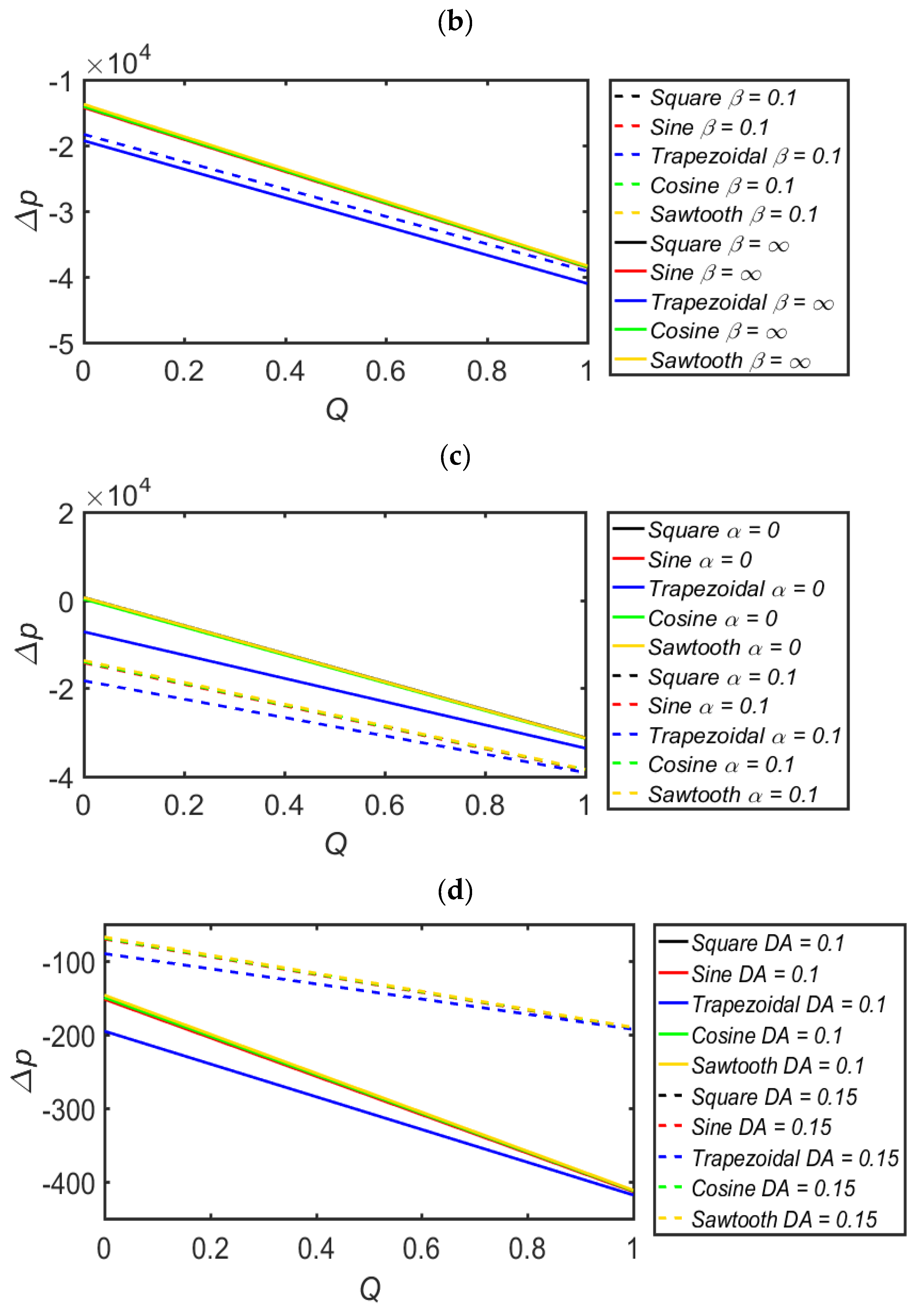Figure 5b illustrates that, with an increase in the time relaxation parameter from 0.1 to $\infty$, the magnitude of the pressure rise decreases. This figure is plotted under porosity and curvature effects. This diagram is plotted for multi-sinusoidal wave frames. Similar behavior is predicted in all these wave frames. The physical impact of a non-uniform parameter on the pressure rise is displayed in Figure 5c. This figure reveals that, with an increasing numeric value of the non-uniform parameter from 0 to 0.1, the pressure rise increases significantly. This figure is plotted under the combined effects of porosity medium and viscoelasticity. Physically, these results show that the non-uniform parameter has a remarkable role in the enhancement of the magnitude of the pressure rise. A similar pattern in the magnitude of the pressure rise is observed in all multi-sinusoidal wave frames. The magnitude of pressure increases with greater porosity effects, as shown in Figure 5d. Additionally, it can be seen that the wave nature of the pressure rise is strongly affected under the larger strength of a porous medium. In all the above figures, it is predicted that the trapezoidal wave has a larger magnitude of pressure rise as compared with all other waveforms (square wave, sine wave, sawtooth wave, and cosine wave), and a smaller magnitude of pressure rise is observed for the sawtooth wave.

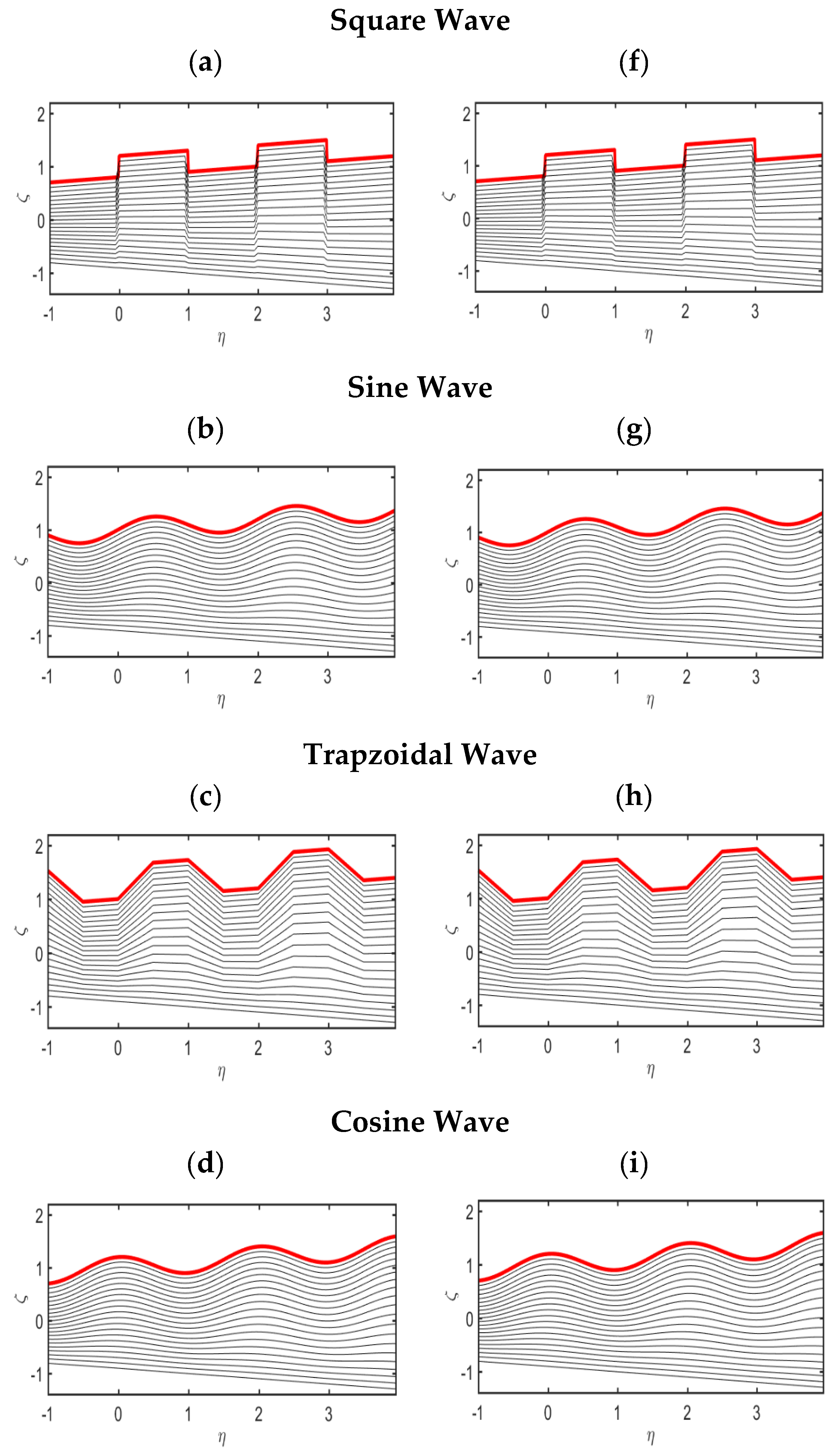
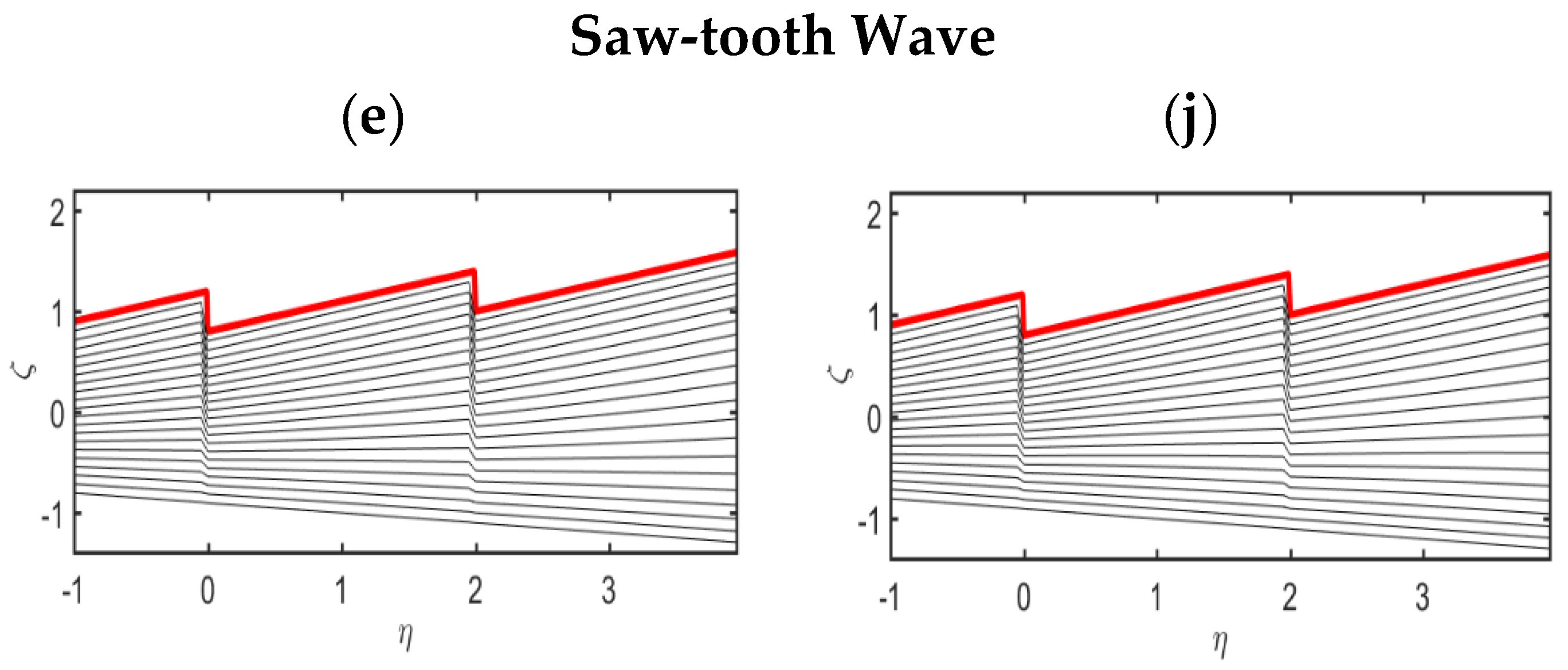
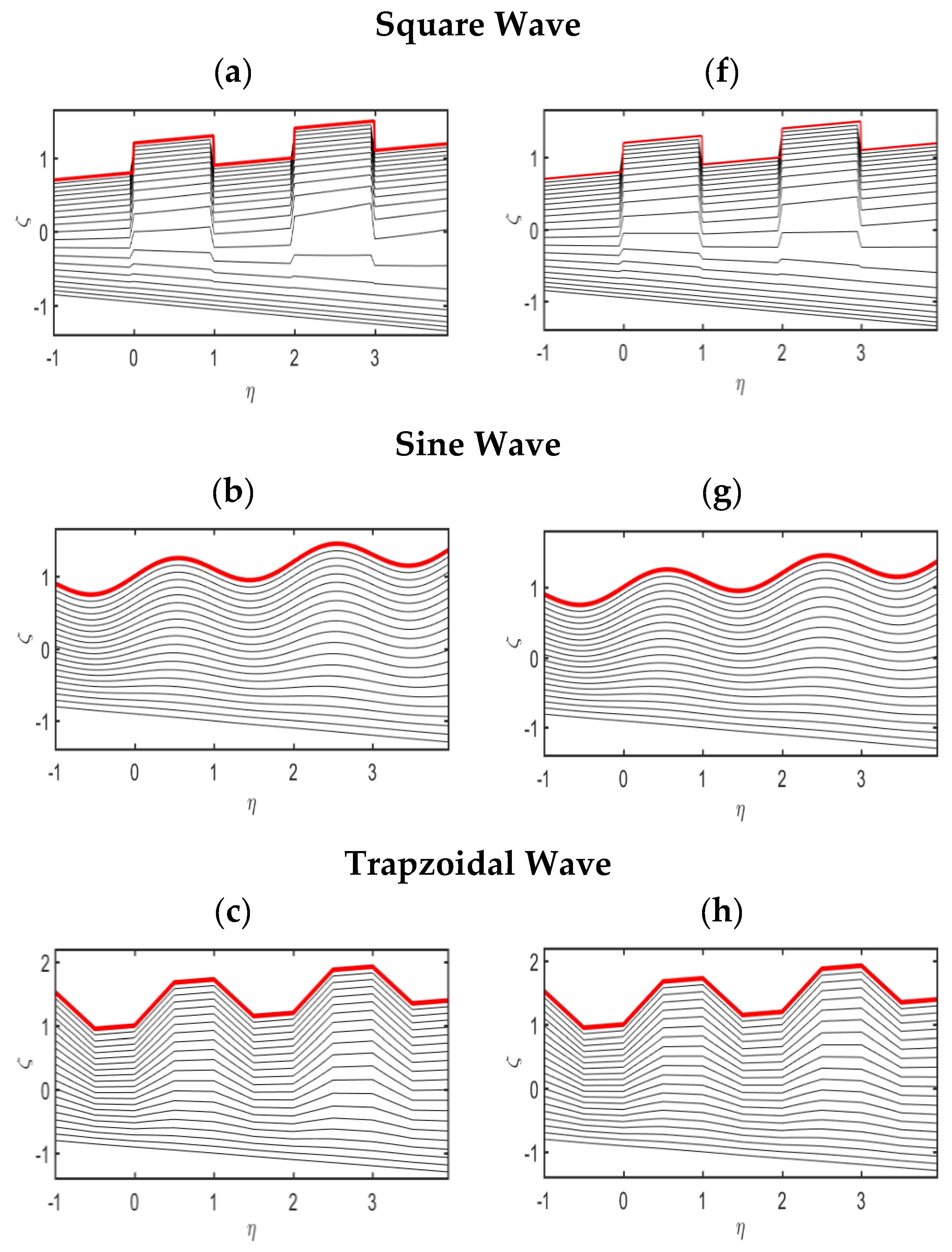
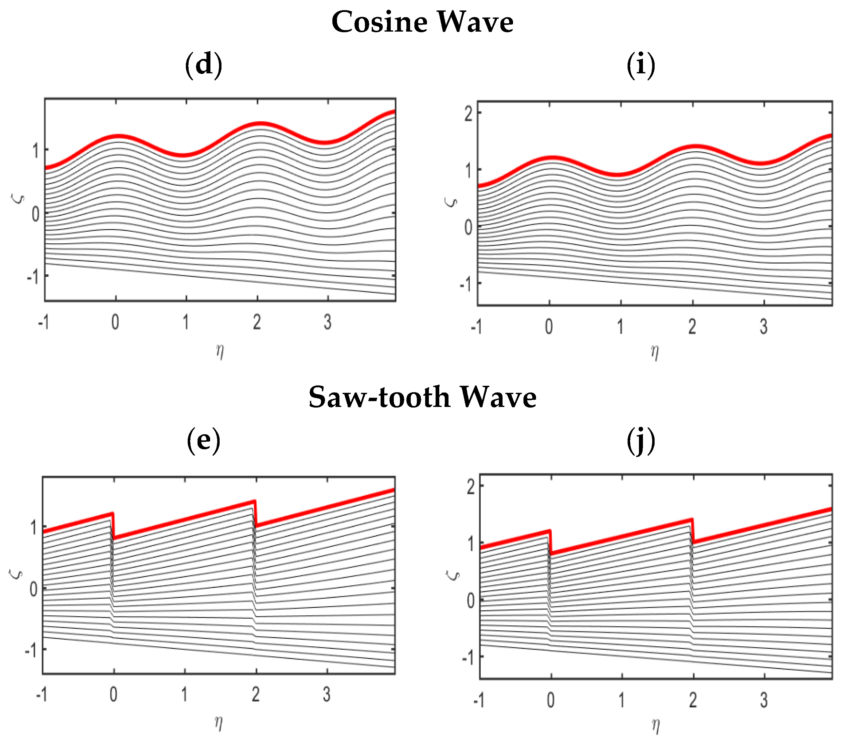
Figure 6, Figure 7, Figure 8 and Figure 9 depict streamlined visualizations for the impact of numerous flow parameters in biomimetic rheology. The physical impacts of the curvature parameter $\left(\sigma \right)$, time relaxation parameter $\left(\beta \right)$, non-uniform parameter $\left(\alpha \right)$, and Darcy’s number $\left(DA\right)$ on the trapping phenomena related to blood rheology, respectively, are presented in Figure 6, Figure 7, Figure 8 and Figure 9. We have plotted these graphs for multi-sinusoidal wave frames at a cross-sectional area, e.g., $q=-2$. 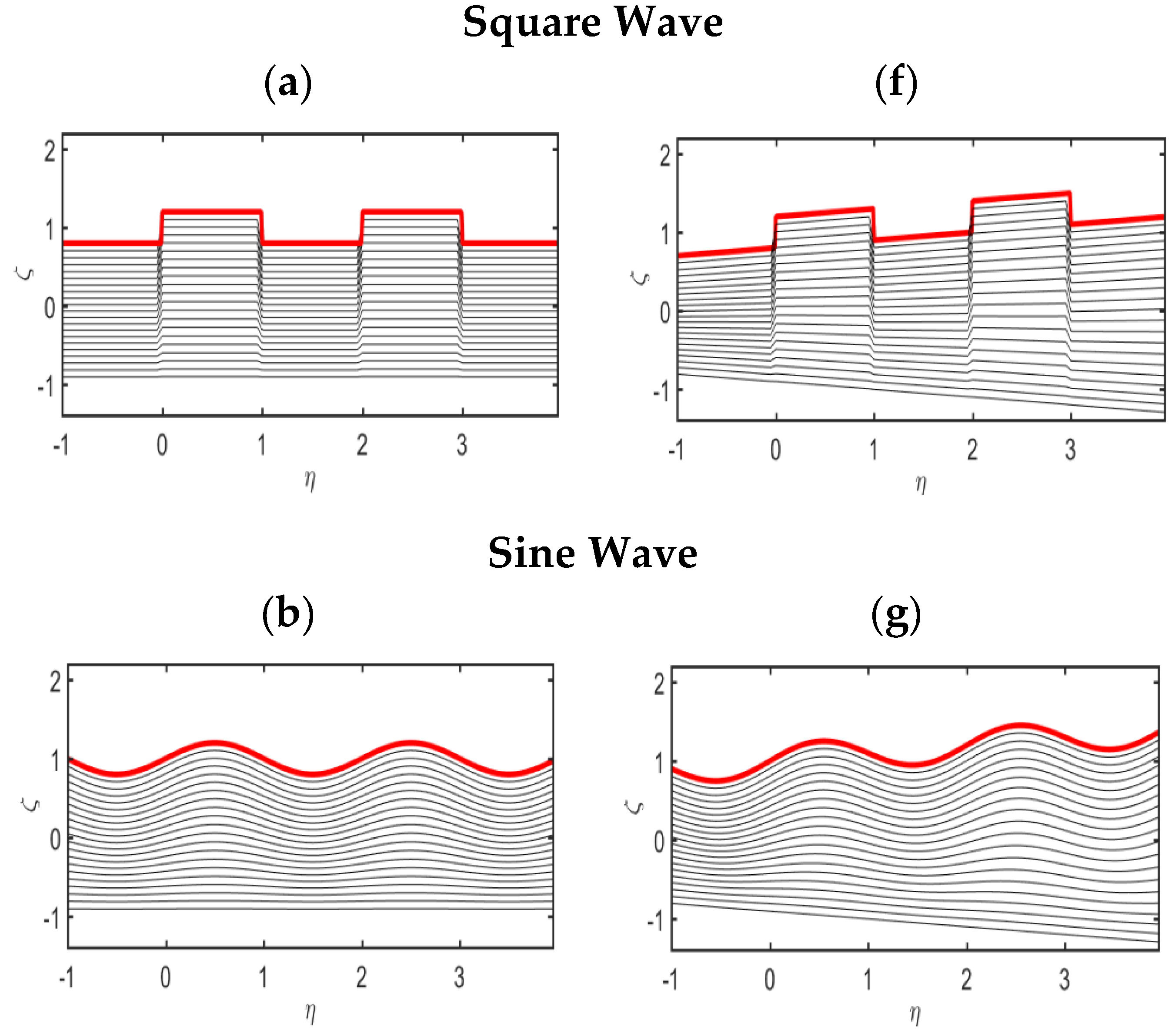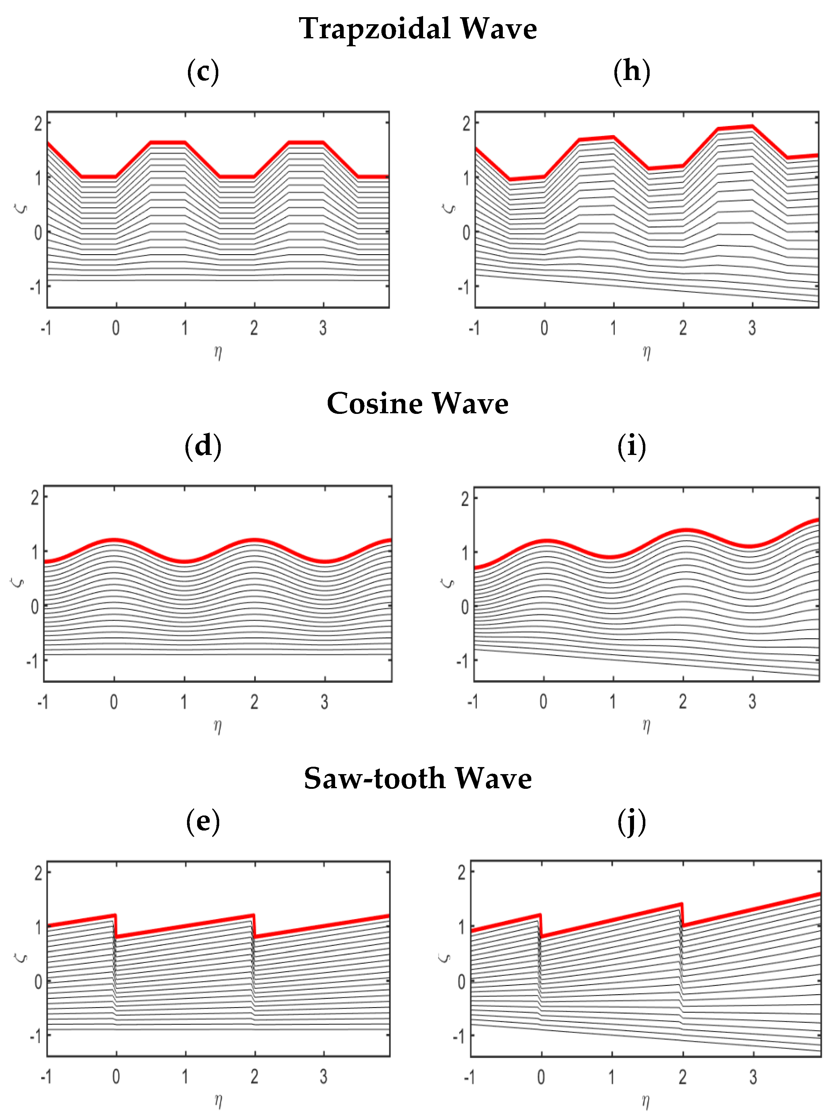Figure 6a–e is plotted for a small numeric value of the radius of curvature, e.g., $\sigma =3$, and the result of a curved pump is obtained. Figure 6f–j is plotted for the largest numeric value of a radius of curvature, e.g., $\sigma \to \infty$, and the results of a straight pump are obtained. These figures are plotted under the combined effects of non-uniform parameter, porous medium, and time relaxation parameter. These figures are plotted for multi-sinusoidal wave frames and are clearly observed from the wave present in each figure of the stream function. The physical behavior of streamlines in both straight and curved pumps is almost the same in shape. 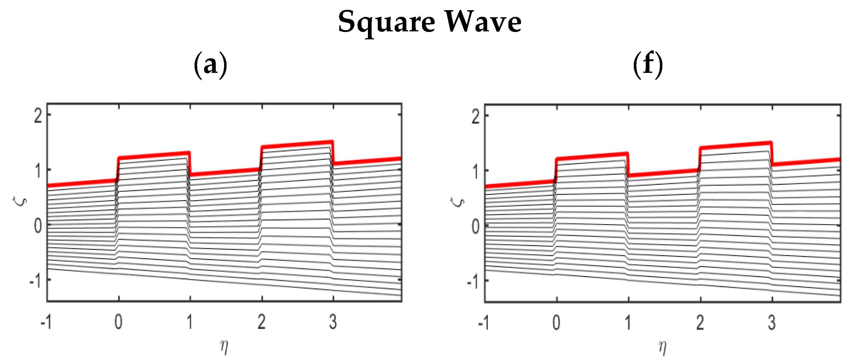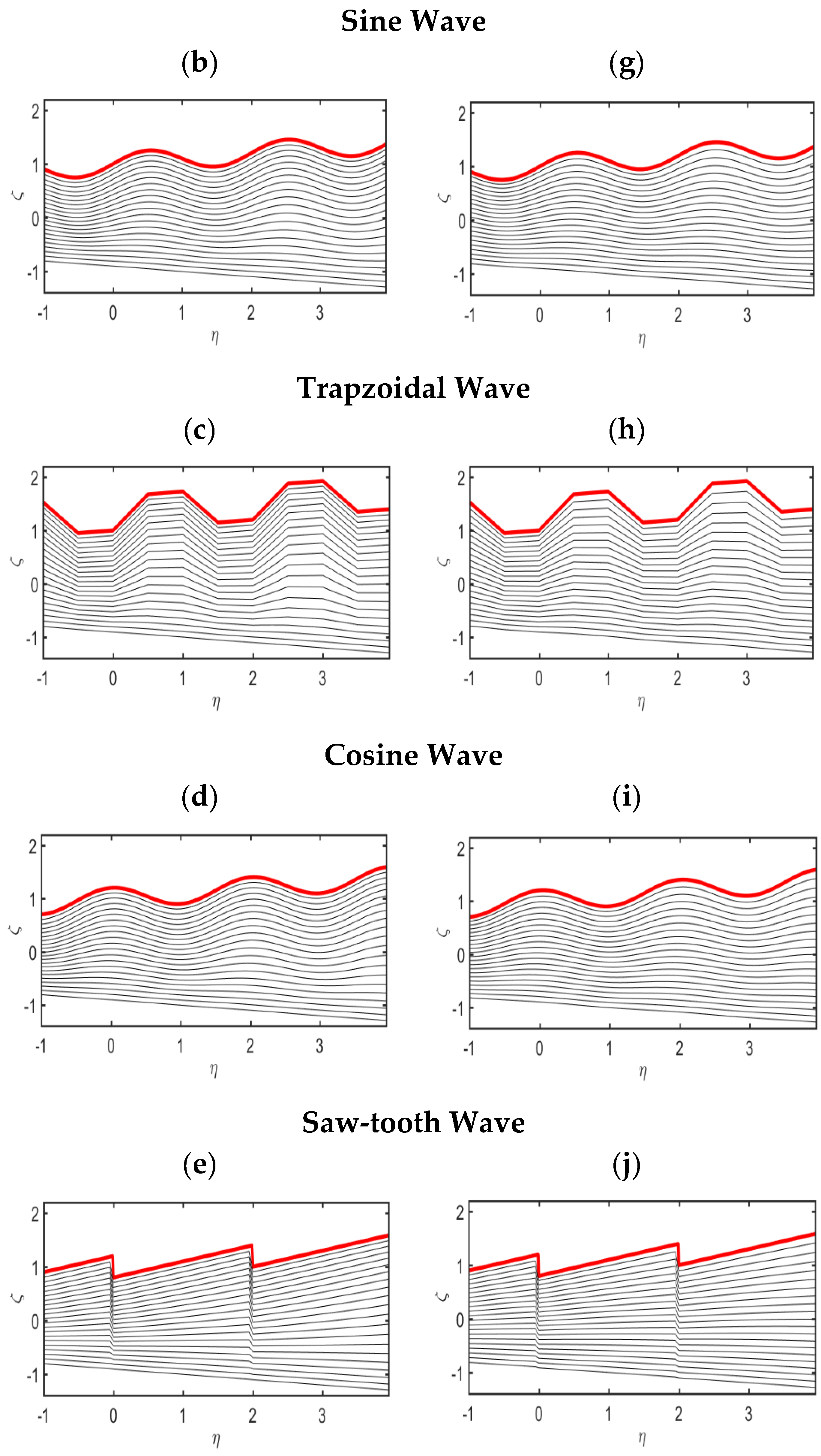Figure 7a–e is plotted for a small numeric value of the viscoelastic parameter, e.g., $\beta =0.1$, for a curved pump. Figure 7f–j is plotted for a large numeric value of the viscoelastic parameter, e.g., $\beta \to \infty$. These figures are plotted under the combined effects of non-uniform parameter, porous medium, and curvature parameter. These figures are plotted for multi-sinusoidal wave frames and are clearly observed from the wave present in each figure of the stream function. The physical behavior of streamlines in both a smaller and larger strength of the time relaxation parameter on the curved pumps is almost the same in shape. The results of viscous liquid are obtained from $\beta =0$. Figure 8a–e is plotted for a uniform parameter, e.g., $\alpha =0$. Figure 8f–j is plotted for a non-uniform parameter, e.g., $\alpha =0.1$. These figures are plotted under the combined effects of a viscoelastic parameter (time relaxation parameter), porous medium, and curvature parameter. These figures are plotted for multi-sinusoidal wave frames and are clearly observed from the wave present in each figure of the stream function. These graphs show that the non-uniform parameter has a dynamic impact in enhancing the length of the streamlines. Figure 9a–e is plotted for a small numeric value of Darcy’s number, e.g., $DA=0.01$, for a curved pump. Figure 9f–j is plotted for a large numerical value of Darcy’s number, e.g., $DA=10$.

These figures are plotted under the combined effects of non-uniform, viscoelastic, and curvature parameters. These figures are plotted for multi-sinusoidal wave frames and are clearly observed from the wave present in each figure of the stream function. The physical behavior of streamlines in both a smaller and larger strength of porosity parameter on the curved pumps are almost the same in shape.

4. Conclusions

A mathematical formulation of the biomimetic rheology in a non-uniform curved pump was performed. The whole mathematical formulation was performed under the creeping phenomena and long wavelength assumption. The transportation of blood through a curved pump was controlled by forces such as a porous medium, the strength of viscoelastic parameter, and a non-uniform parameter. Due to the non-uniform nature of the rheological regime, curvilinear coordinates were used to derive the equations of motion. We have plotted all the figures for multi-sinusoidal wave frames such as square wave, sine wave, trapezoidal wave, cosine wave, and sawtooth wave. Some numerical computations are given below:

➣

The axial velocity is strongly affected with the increasing strength of the porous medium and the viscoelastic nature of fluid. The parabolic shape in the velocity profile is observed for a smaller strength of a porous medium and a smaller numeric value of the time relaxation parameter. BL is predicted for a larger strength of a porous medium and greater numeric values of time relaxation parameter. The sawtooth wave has a larger magnitude of axial velocity as compared with all other wave frames in curved and straight pumps. The non-uniform parameter played a large role in the augmentation of the magnitude of the velocity profile.

➣

Each form of sinusoidal wave can easily be predicted in the graphs of pressure gradients. The straight pump has a larger pressure gradient in magnitude as compared with the curved pump. The magnitude of the pressure gradient is strongly affected under larger strength porosity effects. The non-uniform curved pump has a larger pressure gradient as compared with the uniform curved pump.

➣

The curved pumps have a larger magnitude of peristaltic pumping as compared with the straight pump. The larger strength of the porous medium and non-uniform parameter have a vital role in enhancing peristaltic pumping. Reverse behavior is noticed for a larger strength of viscoelastic effects.

➣

The magnitude of streamlines for a trapezoidal wave is much larger as compared with all other peristaltic wave frames. The length of streamlines is increased by increasing the non-uniform parameter. Similar behavior in the streamlines is noticed for both straight and curved pumps.

➣

The physical results of a non-uniform straight pump are retrieved at smaller values of $\sigma$.

➣

The physical results of a uniform straight pump are retrieved at smaller values of $\sigma$ at $\alpha =0$.

➣

The results of viscous liquid are attained at $\beta =0$.

➣

The results of Tanveer et al. [28] are obtained using a cosine wave frame only at $\alpha =\beta =0$ and $DA\to \infty$.

Some more recent contributions are mentioned in references [27,28,29].

References

1. Mangan, E.V.; Kingsley, D.A.; Quinn, R.D.; Chiel, H.J. Development of a peristaltic endoscope. In Proceedings of the Proceedings 2002 IEEE International Conference on Robotics and Automation (Cat. No. 02CH37292), Washington, DC, USA, 11–15 May 2002; Volume 1, pp. 347–352. [Google Scholar]
2. Mishra, M.; Rao, A.R. Peristaltic transport in a channel with a porous peripheral layer: Model of a flow in gastrointestinal tract. J. Biomech. 2005, 38, 779–789. [Google Scholar] [CrossRef] [PubMed]
3. Lew, H.; Fung, Y.; Lowenstein, C. Peristaltic carrying and mixing of chyme in the small intestine (an analysis of a mathematical model of peristalsis of the small intestine). J. Biomech. 1971, 4, 297–315. [Google Scholar] [CrossRef]
4. Latham, T.W. Fluid Motions in a Peristaltic Pump. Ph.D. Thesis, Massachusetts Institute of Technology, Cambridge, MA, USA, 1966. [Google Scholar]
5. Shapiro, A.H.; Jaffrin, M.Y.; Weinberg, S.L. Peristaltic pumping with long wavelengths at low Reynolds number. J. Fluid Mech. 1969, 37, 799–825. [Google Scholar] [CrossRef]
6. Hayat, T.; Ali, N.; Asghar, S. Hall effects on peristaltic flow of a Maxwell fluid in a porous medium. Phys. Lett. A 2007, 363, 397–403. [Google Scholar] [CrossRef]
7. Javid, K.; Ali, N.; Sajid, M. Simultaneous effects of viscoelasticity and curvature on peristaltic flow through a curved channel. Meccanica 2016, 51, 87–98. [Google Scholar] [CrossRef]
8. Abbasi, F.M.; Zahid, U.M.; Akbar, Y.; Saba; Hamida, M.B.B. Thermodynamic analysis of electroosmosis regulated peristaltic motion of Fe3O4–Cu/H2O hybrid nanofluid. Int. J. Mod. Phys. B 2022, 2250060. [Google Scholar] [CrossRef]
9. Abd-Alla, A.; Abo-Dahab, S. Magnetic field and rotation effects on peristaltic transport of a Jeffrey fluid in an asymmetric channel. J. Magn. Magn. Mater. 2015, 374, 680–689. [Google Scholar] [CrossRef]
10. Ellahi, R.; Bhatti, M.M.; Pop, I. Effects of hall and ion slip on MHD peristaltic flow of Jeffrey fluid in a non-uniform rectangular duct. Int. J. Numer. Methods Heat Fluid Flow 2016, 26, 1802–1820. [Google Scholar] [CrossRef]
11. Bhatti, M.; Ellahi, R.; Zeeshan, A. Study of variable magnetic field on the peristaltic flow of Jeffrey fluid in a non-uniform rectangular duct having compliant walls. J. Mol. Liq. 2016, 222, 101–108. [Google Scholar] [CrossRef]
12. Tripathi, D.; Bég, O.A. A study on peristaltic flow of nanofluids: Application in drug delivery systems. Int. J. Heat Mass Transf. 2014, 70, 61–70. [Google Scholar] [CrossRef]
13. Javid, K.; Al-Khaled, K.; Hassan, M.; Khan, S.U.-D.; Ahmad, A.; Khan, S. A transport of Jeffrey model viscoelastic fluid by complex peristalsis motion of nonuniform curved channel’s walls under resistance of magnetic field. ZAMM-J. Appl. Math. Mech. Für Angew. Math. Mech. 2021, e202100067. [Google Scholar] [CrossRef]
14. Javid, K.; Waqas, M.; Asghar, Z.; Ghaffari, A. A theoretical analysis of Biorheological fluid flowing through a complex wavy convergent channel under porosity and electro-magneto-hydrodynamics effects. Comput. Methods Programs Biomed. 2020, 191, 105413. [Google Scholar] [CrossRef] [PubMed]
15. Javid, K.; Asghar, Z.; Ur Rehman, F. Biomechanics of electro-kinetically modulated peristaltic motion of bio-fluid through a divergent complex wavy channel. Can. J. Phys. 2021, 99, 70–79. [Google Scholar] [CrossRef]
16. Akram, S.; Saleem, N. Analysis of heating effects and different wave forms on peristaltic flow of Carreau fluid in rectangular duct. Adv. Math. Phys. 2020, 2020, 8294318. [Google Scholar] [CrossRef]
17. Akram, S.; Nadeem, S. Significance of nanofluid and partial slip on the peristaltic transport of a non-Newtonian fluid with different wave forms. IEEE Trans. Nanotechnol. 2014, 13, 375–385. [Google Scholar] [CrossRef]
18. Javid, K.; Ali, N.; Asghar, Z. Rheological and magnetic effects on a fluid flow in a curved channel with different peristaltic wave profiles. J. Braz. Soc. Mech. Sci. Eng. 2019, 41, 483. [Google Scholar] [CrossRef]
19. Asghar, Z.; Ali, N. A mathematical model of the locomotion of bacteria near an inclined solid substrate: Effects of different waveforms and rheological properties of couple-stress slime. Can. J. Phys. 2019, 97, 537–547. [Google Scholar] [CrossRef]
20. Hayat, T.; Ali, N.; Asghar, S. An analysis of peristaltic transport for flow of a Jeffrey fluid. Acta Mech. 2007, 193, 101–112. [Google Scholar] [CrossRef]
21. Kothandapani, M.; Srinivas, S. Peristaltic transport of a Jeffrey fluid under the effect of magnetic field in an asymmetric channel. Int. J. Non-Linear Mech. 2008, 43, 915–924. [Google Scholar] [CrossRef]
22. Ramesh, K.; Tripathi, D.; Bég, O.A.; Kadir, A. Slip and hall current effects on Jeffrey fluid suspension flow in a peristaltic hydromagnetic blood micropump. Iran. J. Sci. Technol. Trans. Mech. Eng. 2019, 43, 675–692. [Google Scholar] [CrossRef]
23. Ali, N.; Javid, K.; Sajid, M.; Anwar Bég, O. Numerical simulation of peristaltic flow of a biorheological fluid with shear-dependent viscosity in a curved channel. Comput. Methods Biomech. Biomed. Engin. 2016, 19, 614–627. [Google Scholar] [CrossRef]
24. Ali, N.; Sajid, M.; Abbas, Z.; Javed, T. Non-Newtonian fluid flow induced by peristaltic waves in a curved channel. Eur. J. Mech.-B Fluids 2010, 29, 387–394. [Google Scholar] [CrossRef]
25. Asghar, Z.; Ali, N.; Ahmed, R.; Waqas, M.; Khan, W.A. A mathematical framework for peristaltic flow analysis of non-Newtonian Sisko fluid in an undulating porous curved channel with heat and mass transfer effects. Comput. Methods Programs Biomed. 2019, 182, 105040. [Google Scholar] [CrossRef] [PubMed]
26. Narla, V.; Tripathi, D.; Bég, O.A. Analysis of entropy generation in biomimetic electroosmotic nanofluid pumping through a curved channel with joule dissipation. Therm. Sci. Eng. Prog. 2020, 15, 100424. [Google Scholar] [CrossRef]
27. Shampine, L.F.; Kierzenka, J.; Reichelt, M.W. Solving boundary value problems for ordinary differential equations in MATLAB with bvp4c. Tutor. Notes 2000, 2000, 1–27. [Google Scholar]
28. Tanveer, A.; Hayat, T.; Alsaedi, A. Numerical simulation for peristalsis of Sisko nanofluid in curved channel with double-diffusive convection. Ain Shams Eng. J. 2021, 12, 3195–32078. [Google Scholar] [CrossRef]
29. Ali, N.; Sajid, M.; Hayat, T. Long wavelength flow analysis in a curved channel. Z. Für Nat. A 2010, 65, 191–196. [Google Scholar] [CrossRef] [Green Version]
Figure 1. Peristaltic pumps.
Mathematics 10 01579 g001
Figure 2. Validation of numerical results with Tanveer et al. [28].
Mathematics 10 01579 g002
Figure 3. (a) The velocity distribution w ( ς ) for curvature parameter ( σ ) at q = 3 ,   D A = 0.01 ,   α = 0.1 ,   β = 0.1 ,   and   ϕ = 0.2 . (b) The velocity distribution w ( ς ) for viscoelastic parameter ( β ) at q = 3 ,   D A = 1 ,   α = 0.1 ,   σ = 1.5 ,   and     ϕ = 0.2 . (c) The velocity distribution w ( ς ) for non-uniform parameter ( α ) at q = 3 ,   D A = 0.01 ,   σ = 1.5 ,   β = 0.1 ,   and     ϕ = 0.2 . (d) The velocity distribution w ( ς ) for porosity parameter ( D A ) at q = 3 ,   β = 0.1 ,   α = 0.1 ,   σ = 1.5 ,   and     ϕ = 0.2 .
Mathematics 10 01579 g003aMathematics 10 01579 g003b
Figure 4. (a) The pressure gradient d p / d η for curvature parameter ( σ ) at q = 1.5 ,   D A = 0.01 ,   α = 0.1 ,   β = 0.5 ,   and     ϕ = 0.2 . (b) The pressure gradient d p / d η for viscoelastic parameter ( β ) at q = 1.5 ,   D A = 0.01 ,   α = 0.1 ,   σ = 3   &   ϕ = 0.2 . (c) The pressure gradient d p / d η for non-uniform parameter ( α ) at q = 1.5 ,   D A = 0.01 ,   σ = 3 ,   β = 0.5 ,   and   ϕ = 0.2 . (d) The pressure gradient d p / d η for porosity parameter ( D A ) at q = 1.5 ,   β = 0.5 ,   α = 0.1 ,   σ = 3 ,   and   ϕ = 0.2 .
Mathematics 10 01579 g004aMathematics 10 01579 g004b
Figure 5. (a) The pressure-rise Δ p for curvature parameter ( σ ) at D A = 0.01 ,   α = 0.1 ,   β = 0.5 ,   and   ϕ = 0.2 . (b) The pressure-rise Δ p for viscoelastic parameter ( β ) at D A = 0.01 ,   α = 0.1 ,   σ = 3 ,   and   ϕ = 0.2 . (c) The pressure-rise Δ p for non-uniform parameter ( α ) at D A = 0.01 ,   σ = 3 ,   β = 0.5 ,   and     ϕ = 0.2 . (d) The pressure-rise Δ p for porosity parameter ( D A ) at β = 0.5 ,   α = 0.1 ,   σ = 3 ,   and     ϕ = 0.2 .
Mathematics 10 01579 g005aMathematics 10 01579 g005b
Figure 6. Trapping phenomena for curvature parameter ( σ = 3 ,   ) using (a,f) square wave, (b,g) sine wave, (c,h) trapezoidal wave, (d,i) cosine wave, (e,j) saw-tooth wave at q = 2 ,   D A = 10 ,   α = 0.1 ,   β = 0.1 ,   and     ϕ = 0.2 .
Mathematics 10 01579 g006aMathematics 10 01579 g006b
Figure 7. Trapping phenomena for viscoelastic parameter ( β = 0.1 ,   100 ) using (a,f) square wave, (b,g) sine wave, (c,h) trapezoidal wave, (d,i) cosine wave, (e,j) saw-tooth wave at q = 2 ,   D A = 10 ,   α = 0.1 ,   σ = 2 ,   and     ϕ = 0.2 .
Mathematics 10 01579 g007aMathematics 10 01579 g007b
Figure 8. Trapping phenomena for non-uniform parameter ( α = 0 ,   0.1 ) using (a,f) square wave, (b,g) sine wave, (c,h) trapezoidal wave, (d,i) cosine wave, (e,j) saw-tooth wave at q = 2 ,   D A = 10 ,   α = 0.1 ,   σ = 3 ,   and   ϕ = 0.2 .
Mathematics 10 01579 g008aMathematics 10 01579 g008b
Figure 9. Trapping phenomena for porosity parameter ( D A = 0.01 ,   0.1 ) using (a,f) square wave, (b,g) sine wave, (c,h) trapezoidal wave, (d,i) cosine wave, (e,j) saw-tooth wave at q = 2 ,   β = 0.1 ,   α = 0.1 ,   σ = 3 ,   and   ϕ = 0.2 .
Mathematics 10 01579 g009aMathematics 10 01579 g009b
Publisher’s Note: MDPI stays neutral with regard to jurisdictional claims in published maps and institutional affiliations.