Article

A Hybrid Arithmetic Optimization and Golden Sine Algorithm for Solving Industrial Engineering Design Problems

1
School of Computer Science and Technology, Hainan University, Haikou 570228, China
2
School of Mathematics and Statistics, Hainan Normal University, Haikou 571158, China
3
Key Laboratory of Data Science and Intelligence Education of Ministry of Education, Hainan Normal University, Haikou 571158, China
4
School of Information Engineering, Sanming University, Sanming 365004, China
5
Faculty of Computer Sciences and Informatics, Amman Arab University, Amman 11953, Jordan
6
School of Computer Science, Universiti Sains Malaysia, Gelugor 11800, Malaysia
7
College of Physics and Information Engineering, Fuzhou University, Fuzhou 350108, China
*
Authors to whom correspondence should be addressed.
Mathematics 2022, 10(9), 1567; https://doi.org/10.3390/math10091567
Submission received: 6 April 2022 / Revised: 28 April 2022 / Accepted: 29 April 2022 / Published: 6 May 2022
(This article belongs to the Special Issue Optimisation Algorithms and Their Applications)

Abstract

:
Arithmetic Optimization Algorithm (AOA) is a physically inspired optimization algorithm that mimics arithmetic operators in mathematical calculation. Although the AOA has an acceptable exploration and exploitation ability, it also has some shortcomings such as low population diversity, premature convergence, and easy stagnation into local optimal solutions. The Golden Sine Algorithm (Gold-SA) has strong local searchability and fewer coefficients. To alleviate the above issues and improve the performance of AOA, in this paper, we present a hybrid AOA with Gold-SA called HAGSA for solving industrial engineering design problems. We divide the whole population into two subgroups and optimize them using AOA and Gold-SA during the searching process. By dividing these two subgroups, we can exchange and share profitable information and utilize their advantages to find a satisfactory global optimal solution. Furthermore, we used the Levy flight and proposed a new strategy called Brownian mutation to enhance the searchability of the hybrid algorithm. To evaluate the efficiency of the proposed work, HAGSA, we selected the CEC 2014 competition test suite as a benchmark function and compared HAGSA against other well-known algorithms. Moreover, five industrial engineering design problems were introduced to verify the ability of algorithms to solve real-world problems. The experimental results demonstrate that the proposed work HAGSA is significantly better than original AOA, Gold-SA, and other compared algorithms in terms of optimization accuracy and convergence speed.

1. Introduction

The main optimization process can be considered to obtain the best solution among all potential solutions according to the various NP-hard and engineering problems. Many real-world problems, such as image processing [1,2,3], engineering design [4,5,6,7,8], and job shop scheduling [9], can be expressed as optimization problems and solved using optimization techniques. In the past two decades, the complexity of real-world optimization problems has increased sharply. However, the traditional (mathematical) methods cannot find the optimal solution or near-optimal solution in many cases [10]. Therefore, many researchers have turned their attention to meta-heuristic algorithms (MAs). Unlike traditional techniques, MAs are flexible and reliable in solving complex optimization problems [11].
Over the past few decades, various MAs had been proposed according to natural phenomena, physical principles, biological behaviors, etc. [12]. MAs can be separated into three main categories (as shown in Figure 1): (1) swarm intelligence-based methods, (2) physics-based methods, and (3) evolution-based methods. The first kind of method mimics the biological entities in nature that have collaboration behavior to finish hunting, migrating, etc. [13]. Developed algorithms in this category are Whale Optimization Algorithm (WOA) [14], Particle Swarm Optimization (PSO) [15], Grey Wolf Optimizer (GWO) [16], Salp Swarm Algorithm (SSA) [17], Ant Lion Optimization (ALO) [18], Moth Flame Optimization (MFO) [19], Slime Mould Algorithm (SMA) [20], Harris Hawks Optimization (HHO) [21], Reptile Search Algorithm (RSA) [22], and Aquila Optimizer (AO) [23]. The second type of method mainly simulates the physical phenomena of the universe and methods designed based on these laws are Multi-Verse Optimizer (MVO) [24], Sine Cosine Algorithm (SCA) [25], Arithmetic Optimization Algorithm (AOA) [26], Golden Sine Algorithm (Gold-SA) [27], Henry Gas Solubility Optimization (HGSO) [28], Gravity Search Algorithm (GSA) [29], Atom Search Optimization (ASO) [30], and Equilibrium Optimizer (EO) [31]. The evolution-based methods stem from the biological evolution process in nature. Some of the well-known algorithms developed by this behavior are Genetic Algorithm (GA) [32], Bio-geography-Based Optimizer (BBO) [33], Differential Evolution (DE) [34], and Evolution Strategy (ES) [35]. However, considering the No-Free-Lunch (NFL) theorem [36], no specific optimization algorithm can solve all real-world problems, which motivates us to design more efficient methods to solve them well.
The Arithmetic Optimization Algorithm (AOA) [26] is a physics-based and gradient-free method proposed by Abualigah et al. in 2021. It originated from the commonly used mathematical operators including Addition (+), Subtraction (−), Multiplication (×), and Division (÷). This approach integrates these four operators to realize different search mechanisms (exploration and exploitation) in the search space. Specifically, AOA uses the high distribution characteristics of (× and ÷) operators to realize the exploration approach. In the same way, the (+ and −) operators are used to obtain the high-dense results (exploitation approach). However, some researches denote that the original AOA has some defects, such as it easily suffering from a local optimal and slow convergence speed. Therefore, many variant versions of AOA were proposed to improve its searchability. For example, Azizi et al. [37] proposed an improved AOA based on Levy flight to determine the steel structure’s optimal fuzzy controller parameters. Agushaka et al. [38] proposed an improved version of AOA called nAOA, which integrated the high-density values and beta distribution to enhance searchability. An Adaptive AOA, called APAOA, was proposed by Wang et al. [39]. In the APAOA, the parallel communication strategy was used to balance the exploration and exploitation ability of the original AOA. Another improved AOA that utilized a hybrid mechanism, named DAOA, was proposed by Abualigah et al. [40]. In DAOA, the differential evolution technique was integrated to enhance the local search ability of AOA, and to help it to jump out of the local optimal solution. Elkasem et al. [41] presented an eagle strategy AOA called ESAOA. In this work, the eagle strategy is used to avoid premature convergence and increase the population’s efficacy to obtain the optimal solution. Sharma et al. [42] introduced an opposition-based AOA namely OBAOA for identifying the parameters of PEMFCs. The opposition-based learning strategy is used to promote the algorithm to find the high-precision solution and improve the convergence rate. Abbassi et al. [43] developed an improved AOA to determine the solar cell parameters. In this work, the new operator called narrowed exploitation was used to narrow the search space and focus on the potential area to find the optimal or near-optimal solutions. Zhang et al. [44] proposed an improved AOA called IAO, which integrated the chaotic theory. The chaotic theory improves the algorithm to escape the optimal solution with a suitable convergence speed. Moreover, the IAO was used to optimize the weight of neural network.
Given the above discussion, some of the variants of AOA have strong searchability, but they cannot converge to the optimal solution at an appropriate time, i.e., they still easily fall into the local optimal solution. Furthermore, by considering the NFL theorem and increasingly complex real-world problems, the development of new and improved versions of MAs is ongoing. In general, a single optimizer also exposes some shortcomings; for example, it neglects to share useful information between populations, which may cause the algorithm to have insufficient search capability. Therefore, many researchers utilized the characteristic of two Mas, i.e., designing a hybrid algorithm to improve performance and applying it to solve complex real-world optimization problems. Unlike the single algorithm, the hybrid algorithm alleviates these shortcomings and increases diversity, and shares more helpful information within the population. Thus, the hybrid algorithm has more powerful searchability than the single algorithm. Gold-SA is a physics-based technique with a good exploitation ability to find the near-optimal solution. Furthermore, Gold-SA also has fewer parameters and is easy to program. Motivated by these considerations, in this paper, we propose an improved hybrid version of AOA called HAGSA that combines both AOA and Gold-SA. The proposed method uses Gold-SA to increase the population diversity and share more useful information between search agents. At the same time, Levy flight and a new strategy called Brownian mutation are used to enhance the exploration and exploitation capability of hybrid algorithms, respectively. To evaluate the effectiveness of the proposed method, we selected the CEC 2014 competition test suite as the benchmark function and compared the results with seven well-known methods, including AOA and Gold-SA. In addition, five classical engineering design problems, including the car side crash design problem, pressure vessel design problem, tension spring design problem, speed reducer design problem, and cantilever beam design problem, were also used to evaluate HAGSA’s ability to solve real-world problems. Experimental results demonstrate that the proposed work can provide complete results and achieve a faster convergence speed compared to other optimizers. The main contributions of this paper are as follows:
  • We propose a new hybrid algorithm based on the Arithmetic Optimization Algorithm and Golden Sine Algorithm (HAGSA).
  • Levy flight and a new mechanism called Brownian mutation are carried out to enhance the exploration and exploitation ability of the hybrid algorithm.
  • The performance of the proposed work is assessed on the CEC 2014 competition test suite and five classical engineering design problems.
  • Several well-known MAs are compared with the proposed method.
  • Experimental results indicate that HAGSA has more reliable performance than that of other well-known algorithms.
The remainder of this paper is structured as follows: Section 2 briefly illustrates the concepts of AOA and Gold-SA. Section 3 describes Levy flight, Brownian mutation, and the details of HAGSA. Section 4 presents and analyzes the experimental results of the proposed work. Finally, this paper’s conclusion and potential research directions are discussed in Section 5.

2. Preliminaries

This section introduces the inspiration and mathematical model of the original AOA and Gold-SA, in turn.

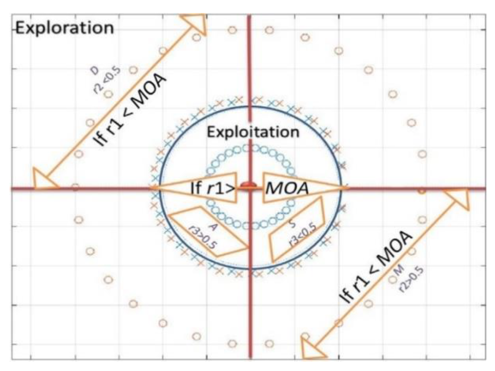
2.1. Arithmetic Optimization Algorithm (AOA)

The theory of AOA is described in this section. The main inspiration of AOA originates from the use of arithmetic operators such as Addition (A), Subtraction (S), Multiplication (M), and Division (D) to solve optimization problems [33]. In the following subsections, we discuss the different influences of these operators on optimization problems and the search method of AOA, as shown in Figure 2.

2.1.1. Initialization Phase

Like other meta-heuristic optimization algorithms, AOA is based on population behavior. The set of a population X containing N search agents is illustrated in Equation (1). In the matrix, each row indicates a search agent [33].
X = [ x 1 , 1 x 1 , j x 1 , n 1 x 1 , n x 2 , 1 x 2 , j x 2 , n x N 1 , 1 x N 1 , j x N 1 , n x N , 1 x N , j x N , n 1 x N , n ]
After generating the population, the fitness of each search agent is computed, and the best one will be determined. Next, AOA decides to perform exploration or exploitation through the Math Optimizer Accelerated (MOA) value, which is defined as follows:
M O A ( t ) = M i n + t × ( M a x M i n T )
where MOA(t) indicates the value of MOA at the t-th iteration. Min and Max denote the minimum and maximum values of the accelerated function, respectively. t denotes the current iteration, and T denotes the maximum iteration. The search agent performs the exploration phase when r1 > MOA, otherwise the exploitation phase will be executed.

2.1.2. Exploration Phase

In this section, the exploration phase of AOA is described. According to the main inspiration, the Division (D) and Multiplication (M) operators are introduced to achieve high distributed values or decisions [33]. The Division and Multiplication operators can be mathematically described as follows:
X i , j ( t + 1 ) = { X b e s t , j ( t ) × M O P × ( ( U B j L B j ) × μ + L B j ) ,   r 2 < 0.5 X b e s t , j ( t ) ÷ ( M O P + ε ) × ( ( U B j L B j ) × μ + L B j ) ,   otherwise
where Xi,j(t + 1) denotes the jth position of the ith solution in the next iteration. Xbest,j(t) denotes the best solution obtained so far in the jth position. LBj and UBj denote the lower and upper boundaries, respectively, of the search space at the jth dimension. ε is a small integer number, and r2 denotes the random value between 0 and 1. μ = 0.5, which represents the control function. Moreover, the Math Optimizer can be calculated as follows:
M O P ( t ) = 1 t 1 / α T 1 / α
where α = 0.5 denotes the dynamic parameter, which determines the accuracy of the exploitation phase throughout iterations.

2.1.3. Exploitation Phase

In this section, we discuss the exploitation phase of AOA. In contrast to the D and M operator, AOA utilizes the Addition (A), and Subtraction (S) operators to derive high density solutions because (S and A) can easily approach the target region due to their low dispersion [33]. The mathematical formula can be described as follows:
X i , j ( t + 1 ) = { X b e s t , j ( t ) M O P × ( ( U B j L B j ) × μ + L B j ) ,   r 3 < 0.5 X b e s t , j ( t ) + M O P × ( ( U B j L B j ) × μ + L B j ) ,   otherwise
where r3 denotes a random value in the range 0 to 1.
The pseudo-code of AOA is illustrated in Algorithm 1.
Algorithm 1 pseudo-code of AOA [33]
  • Input: The parameter of AOA such as control function (μ), dynamic parameter (α), number of search agents (N), and maximum iteration (T)
  • Output: the best solution
  • Initialize the search agent randomly.
  • While (t < T) do
  •    Check if any search agent goes beyond the search space and amend it.
  •    Calculate fitness for the given search agent.
  •    Update the MOA and MOP using Equations (2) and (4), respectively.
  •    For i = 1 to N do
  •      For j = 1 to D do
  •         Update the random value r1, r2, r3.
  •         If r1 > MOA then
  •           If r2 > 0.5 then
  •               Update position by Division (÷) operator in Equation (3).
  •           Else
  •               Update position by Multiplication (×) operator in Equation (3).
  •           End if
  •       Else
  •           If r3 > 0.5 then
  •               Update position by Addition (+) operator in Equation (5).
  •         Else
  •               Update position by Subtraction (−) operator in Equation (5).
  •         End if
  •       End if
  •     End for
  •    End for
  •    t = t + 1.
  • End while

2.2. Golden Sine Algorithm (Gold-SA)

This section introduces the basic theory of the Golden Sine Algorithm (Gold-SA). The inspiration of Gold-SA is a sine function in mathematics, and the individuals explore the approximate optimal solution in the search space according to the golden ratio [27]. The range of the sine function is [−1, 1], with period 2π. When the value of x1 changes, the corresponding variable y1 also changes. Combining the sine function and golden ratio helps to continuously reduce the search space and search in regions where the optimal values are more likely to be generated, thereby improving the convergence speed [27]. The calculation formula is as follows:
X i , j ( t + 1 ) = X i , j ( t ) × | sin ( p 1 ) | p 2 × sin ( p 1 ) × | d 1 × X b e s t , j ( t ) d 2 × X i , j ( t ) |
where p1 is the random value between [0, 2π], and p2 is the random between [0, π], and d1 and d2 are the coefficient factors, which are obtained by the following equation:
d 1 = a × τ + b × ( 1 τ )
d 2 = a × ( 1 τ ) + b × τ
where a and b are the initial values, which are −π and π. τ denotes the golden ratio, which is ( 5 1 ) / 2 . The pseudo-code of Gold-SA is shown in Algorithm 2.
Algorithm 2 pseudo-code of Gold-SA [27]
  • Input: The parameter of Gold-SA, such as the number of search agents (N), and maximum iteration (T).
  • Output: The best solution
  • Initialize the search agent randomly.
  • While (t < T) do
  •     Check if any search agent goes beyond the search space and amend it.
  •     Calculate fitness for the given search agent.
  •     For i = 1 to N do
  •         Update the random value p1 and p2, respectively.
  •         For j = 1 to D do
  •             Update position of search agent by the Equation (6).
  •         End for
  •     End for
  •     t = t + 1.
  • End while

3. The Proposed Algorithm
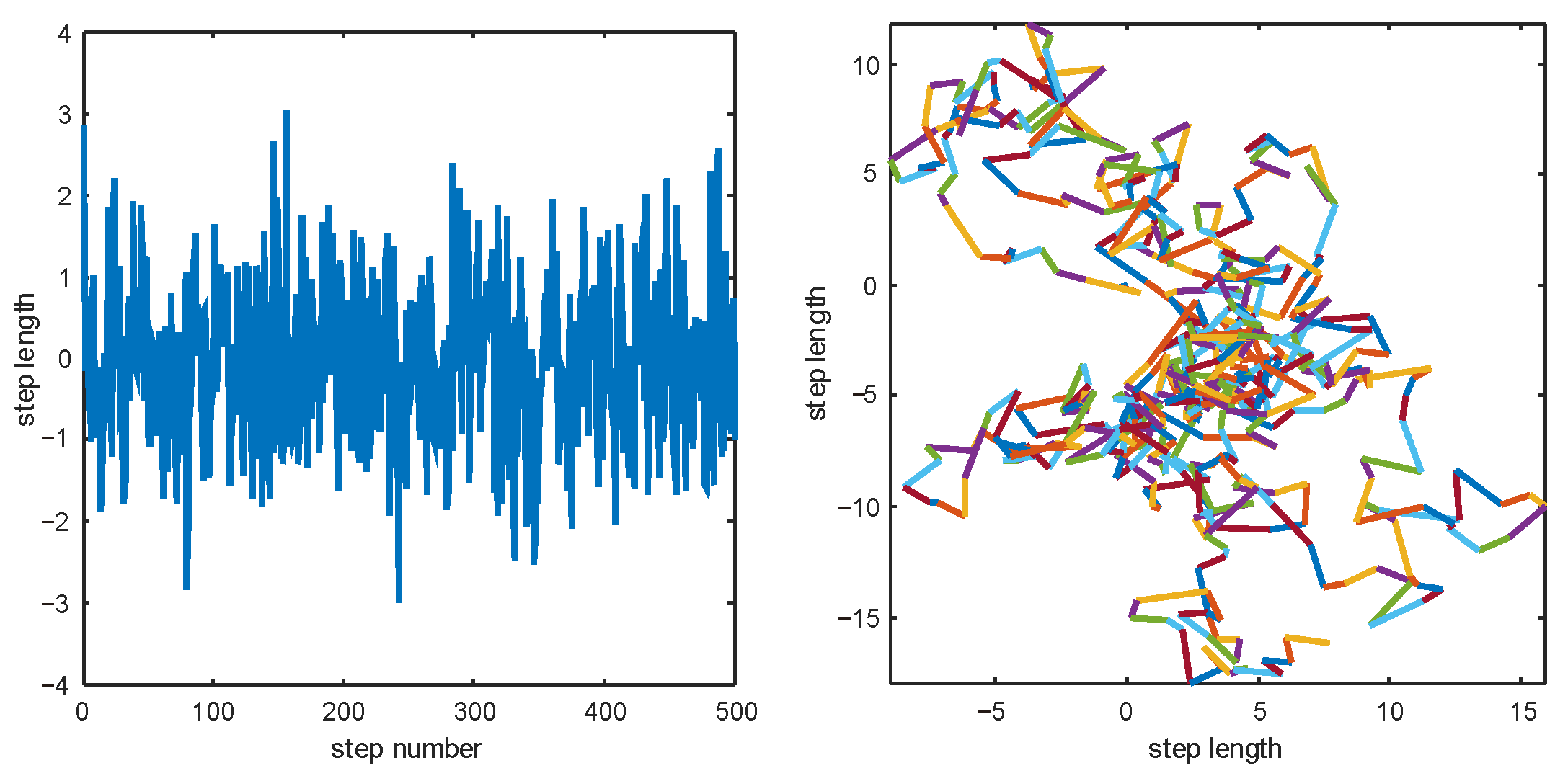
In this section, we describe the proposed method. First, Levy flight is presented. Second, we propose a new strategy called Brownian mutation. Then, the details of the proposed work, HAGSA, are discussed and analyzed.

3.1. Levy Flight

Numerous studies reveal that the flight trajectories of many flying animals are consistent with characteristics typical of Levy flight. Levy flight is a class of non-Gaussian random walk that follows the Levy distribution [41,42]. It performs occasional long-distance walking with frequent short-distance steps, as shown in Figure 3. The mathematical formula for Levy flight is as follows:
L e v y = 0.01 × r 4 × σ | r 5 | 1 β
σ = ( Γ ( 1 + β ) × sin ( π β 2 ) Γ ( 1 + β 2 ) × β × 2 ( β 1 2 ) ) 1 β
where r4 and r5 are random values between [0, 1], and β is a constant equal to 1.5.

3.2. Brownian Mutation

This paper proposes a Brownian mutation mechanism based on the mutation operator and Brownian motion. In 1995, differential evolution (DE) was proposed by Storn et al. [34], which was inspired by the mutation, crossover, and selection mechanisms in nature. Thus, DE obtains the optimal or near-optimal solution according to these operators. However, the crossover and mutation operators generate only one candidate solution in each iteration, limiting the population diversity and searchability of MAs [8]. Brownian motion (BM) is a stochastic process with a step size derived from a probability function defined by a normal distribution with μ = 0 and σ2 = 1 [43]. The formula of BM is listed as follows:
f B ( x ; μ , σ ) = 1 2 π σ 2 exp ( ( x μ ) 2 2 σ 2 ) = 1 2 π exp ( x 2 2 )
where x indicates a point following this motion, and the distribution and 2D trajectory of BM as shown in Figure 4. We can see that BM’s trajectory can explore distant areas of the neighborhood, which shows more efficiency than a uniform random search in the search space. Therefore, considering the high performance of Brownian motion and the limitation of the mutation operator, we propose Brownian mutation, which generates two trail vectors with the Brownian motion strategy. This method generates two candidate solutions V1 and V2 of the i-th search agent in parallel through Equations (12) and (13), respectively.
The first mutation candidate solution V1 is calculated as follows:
V 1 , j = { X r 6 ( t ) + B r o w n i a n × ( X r 7 ( t ) X r 8 ( t ) ) , if   r a n d ( ) < m r 1 X i , j , otherwise
where r6, r7, and r8 denote random values between 0 and 1. mr1 is the mutation rate, and its value is 0.3. Brownian indicates the Brownian motion.
The second mutation candidate solution V2 is calculated as follows:
V 2 , j = { X b e s t ( t ) + B r o w n i a n × ( X r 9 ( t ) X r 10 ( t ) ) , if   r a n d ( ) < m r 2 X i , j , otherwise
where r9, r10, and r11 denote random values between 0 and 1. mr2 is the mutation rate equal to 0.5.
When two candidate solutions V1 and V2 are generated, they are first modified according to the lower and upper boundaries. Then, the best candidate solution Vbest is selected using Equation (14) (lowest fitness as the criterion).
V b e s t = { V 1 ,   if   f ( V 1 ) < f ( V 2 ) V 2 ,   otherwise
Afterward, the best solution between Vbest and Xi is selected as the ith search agent in the next iteration. The following equation describes this behavior:
X i = { V b e s t , if   f ( V b e s t )   <   f ( X i ) X i , otherwise

3.3. The Details of HAGSA

As mentioned above, single MAs have low diversity and cannot share useful information within the population. Moreover, the original AOA has shortcomings, such as easily stagnating into optimal local solutions and slow convergence speed. The Gold-SA has strong local searchability in the search space. Thus, to overcome the disadvantages of the original AOA and take full advantage of the benefits of Gold-SA, in this paper, we present a hybrid algorithm based on the AOA and Gold-SA, namely HAGSA. We divided the whole population into two subgroups, Group A and Group B, and optimized them using AOA and Gold-SA, respectively. Integrating both AOA and Gold-SA can increase population diversity and all the exchange pf useful search information between search agents. This operation aims to enable search agents to find the valuable solution in the search space based on two MAs (AOA and Gold-SA) in less time and increase the diversity throughout the entire iterations. Furthermore, to enhance the searchability of the hybrid algorithm, it was integrated with Levy flight and Brownian mutation. Levy flight can improve the hybrid algorithm’s exploration ability, allowing search agents to explore more potential regions in the search space. Thus, the improved exploration phase can be calculated by Equation (16). Furthermore, the Brownian mutation is used to strengthen the exploitation capability of the hybrid algorithm and help the individuals escape the local optimal solution.
X i , j ( t + 1 ) = { X b e s t , j ( t ) × L e v y ( j ) × M O P × ( ( U B j L B j ) × μ + L B j ) ,   r 2 < 0 . 5 X b e s t , j ( t ) × L e v y ( j ) ÷ ( M O P + ε ) × ( ( U B j L B j ) × μ + L B j ) ,   otherwise
The pseudo-code of HAGSA is expressed in Algorithm 3, and the flowchart of the proposed work is shown in Figure 5.
Algorithm 3 pseudo-code of HAGSA
  • Input: The parameter such as control function (μ), dynamic parameter (α), number of search agent (N), and maximum iteration (T).
  • Output: best solution
  • Initialize the search agent randomly.
  • While (t < T) do
  •     Check if any search agent goes beyond the search space and amend it.
  •     Calculate fitness for the given search agent.
  •     Update the MOA and MOP using Equations (2) and (4), respectively.
  •     For i = 1 to N do
  •         For j = 1 to D do
  •             Update the random value r1, r2, r3.
  •             If i < N/2 then
  •                 If r1 > MOA then
  •                     If r2 > 0.5 then
  •                         Update position by Division (÷) operator in Equation (16).
  •                     Else
  •                         Update position by Multiplication (×) operator in Equation (16).
  •                     End if
  •                 Else
  •                     If r3 > 0.5 then
  •                         Update position by Addition (+) operator in Equation (5).
  •                     Else
  •                         Update position by Subtraction (−) operator in Equation (5).
  •                     End if
  •                 End if
  •             Else
  •                 Update position by Gold-SA operator in Equation (6).
  •             End if
  •             Generate candidate solution V1 and V2 by Equations (12) and (13).
  •             Check if V1 and V2 goes beyond the search space and amend it.
  •             Choose the best solution as Vbest with the lower fitness from V1 and V2.
  •             If f(Vbest) < f(Xi) then
  •                 Xi = Vi.
  •                 End if
  •             End for
  •         End for
  •         t = t + 1.
  • End while

3.4. Computational Complexity Analysis

In the initialization phase, HAGSA produces the search agents randomly in the search space, so the computational complexity of this phase is O(N × D), where N denotes the number of population and D denotes the dimension size. Afterward, HAGSA evaluates each individual’s fitness during the whole iteration with the complexity O(T × N × D), where T indicates the number of iterations. Finally, we used AOA, Gold-SA, Levy flight, and Brownian mutation to obtain the best solution. Thus, the computational complexities of these phases are O(3 × T × N × D). In summary, the total computational complexity of HAGSA is O(T × N × D).

4. Experimental Results and Discussion

This section evaluates the effectiveness of the proposed HAGSA algorithm using the CEC 2014 competition test suite and five industrial engineering design problems. First, the benchmark functions and experimental setup are described. Next, the statistical results of the CEC 2014 benchmark functions are analyzed and discussed. Finally, the five industrial engineering design problems are used to prove the advantages of HAGSA.

4.1. Definition of CEC 2014 Benchmark Functions

To validate the searchability of the proposed HAGSA, we considered the CEC 2014 competition test suite as a benchmark function to evaluate the performance of HAGSA and its peers, which include 30 extremely complex functions [44]. The details of the benchmark functions are listed in Table 1, where fmin denotes the theoretical optimal fitness. According to their characteristics, the CEC 2014 test suite can be categorized into four classes. C01–C03 are unimodal functions with only one global optimum without any local optima, and are suitable for evaluating algorithms’ exploitation capability. C04–C15 are multimodal functions with only one global optimal value with many local optimal values, and can evaluate algorithms’ exploration and local minima avoidance ability. C16–C22 are hybrid functions, including both unimodal and multimodal functions, and can simultaneously examine the exploration and exploitation capability of algorithms. C23–C30 are composition functions that maintain continuity around the local and global optima. All these functions are rotated and shifted, so their complexity increases dramatically. Figure 6 provides a 2D visualization of some functions of the CEC 2014 test suite to understand its characteristics.

4.2. Experimental Setup

As stated above, the CEC 2014 test suite was utilized to evaluate HAGSA’s optimization performance. To demonstrate the validity of the experimental results, the proposed algorithm HAGSA was compared with the basic AOA [26], Gold-SA [27], Remora Optimization Algorithm (ROA) [45], Aquila Optimizer (AO) [23], Sine Cosine Algorithm (SCA) [25], Whale Optimization Algorithm (WOA) [14], Flower Pollination Algorithm (FPA) [46], Differential Evolution (DE) [8], and Genetic Algorithm (GA) [47]. We set the maximum iteration T = 500, population size N = 50, dimension size D = 30, and 30 independent runs. The best results are highlighted in bold. All the experiments were conducted on a PC with an Intel (R) Core (TM) i5-11300H CPU @ 3.10 GHz, 16 GB RAM, Windows 10, and MATLAB R2016b. Table 2 denotes the parameter setting of algorithms, and the details of the compared algorithms can be listed as follows:
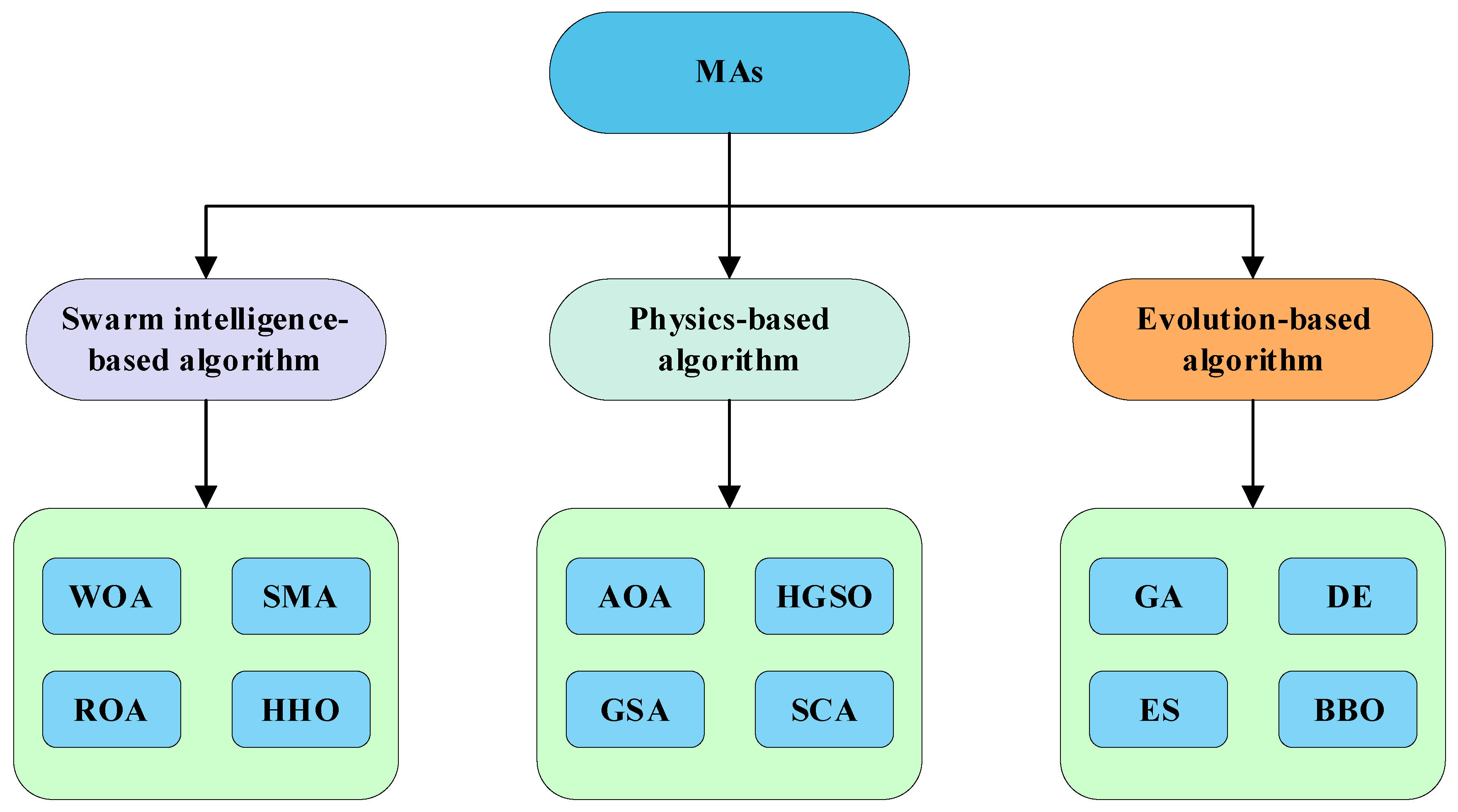
  • AOA: simulates four commonly used arithmetic operators as Division (÷), Multiplication (×), Subtraction (−), and Addition (+).
  • Gold-SA: inspired by the sine function with the golden section search in mathematics compute.
  • ROA: simulates remora’s parasitism behavior on different hosts including whales and swordfish during the hunting process.
  • AO: inspired by Aquila’s four different hunting methods.
  • SCA: simulates the distribution characteristics of sine and cosine functions.
  • WOA: simulates the hunting behavior of humpback whales in oceans.
  • FPA: simulates the pollination process of flowering plants in nature.
  • DE: integrates the differential mutation, crossover, and selection mechanisms.
  • GA: mimics the Darwinian evolution law and biological evolution of genetic mechanism in nature.
Table 2. Parameter setting of each algorithm.
AlgorithmParameters
AOA [26]α = 5; μ = 0.5;
Gold-SA [27]c1 = [1, 0]; c2 ∈ [0, 1]; c3 ∈ [0, 1]
ROA [45]C = 0.1
AO [23]U = 0.00565; r1 = 10; ω = 0.005; α = 0.1; δ = 0.1;
SCA [25]a ∈ [2, 0]
WOA [14]a1 ∈ [2, 0]; a2 ∈ [−1, −2]; b = 1
FPA [46]p = 0.8; β = 1.5
DE [8]Fmin = 0.2; Fmax = 0.8; CR = 0.1
GA [47]Pc = 0.85; Pm = 0.01

4.3. Statistical Results on CEC 2014 Benchmark Functions

Table 3 denotes the mean and standard deviation (std) values obtained by HAGSA and other competed algorithms for each CEC 2014 function with D = 30. According to Table 3, the statistical results illustrate that the HAGSA provides better searchability than its peers. For unimodal functions, HAGSA better obtains the global optimal solution on C01 and C03 than others. For multimodal functions, HAGSA outperforms all other well-known algorithms on nine functions, except functions C07–08, C11, and C14; FPA, DE, ROA, and AO find the global optimal solution for these functions, respectively. For hybrid functions, HAGSA achieves the best results for C16, C19, C20, and C22 among all algorithms. Finally, HAGSA also outperforms the results for composition functions compared to the original AOA, Gold-SA, and other compared algorithms on C23–25 and C28–C30, but not on C26. Figure 7 shows HAGSA and competitor algorithms’ ranking in various functions of the CEC 2014 test suite. In light of these results, HAGSA exhibits excellent performance by obtaining the best average over 21 functions.

4.4. Boxplot Behavior Analysis

The distribution characteristics of data can be displayed through boxplot analysis. The boxplot describes the data distribution as quartiles. The lowest and largest points of the edges of the boxplot are the minimum and maximum values obtained by the algorithm. The lower and upper quartiles are separated by the endpoints of the rectangle [5]. In this subsection, we use boxplot behavior to represent each algorithm’s distribution of the obtained value. Each sample runs 30 times independently for each CEC 2014 benchmark function with D = 30. The boxplot behavior of each algorithm is shown in Figure 8. HAGSA has better stability for most benchmark functions and shows excellent performance compared to the others. In particular, for C01, C04, C05, C08, C09, C12, C13, and C15, the boxplot of the proposed HAGSA method is very narrow compared to others and shows lower values. For C06, C14, and C16, HAGSA achieves the lower values obtained than most algorithms. However, the performance is not obvious when solving C10, C17, C18, C19, C21, C23, C25, C27, and C30.

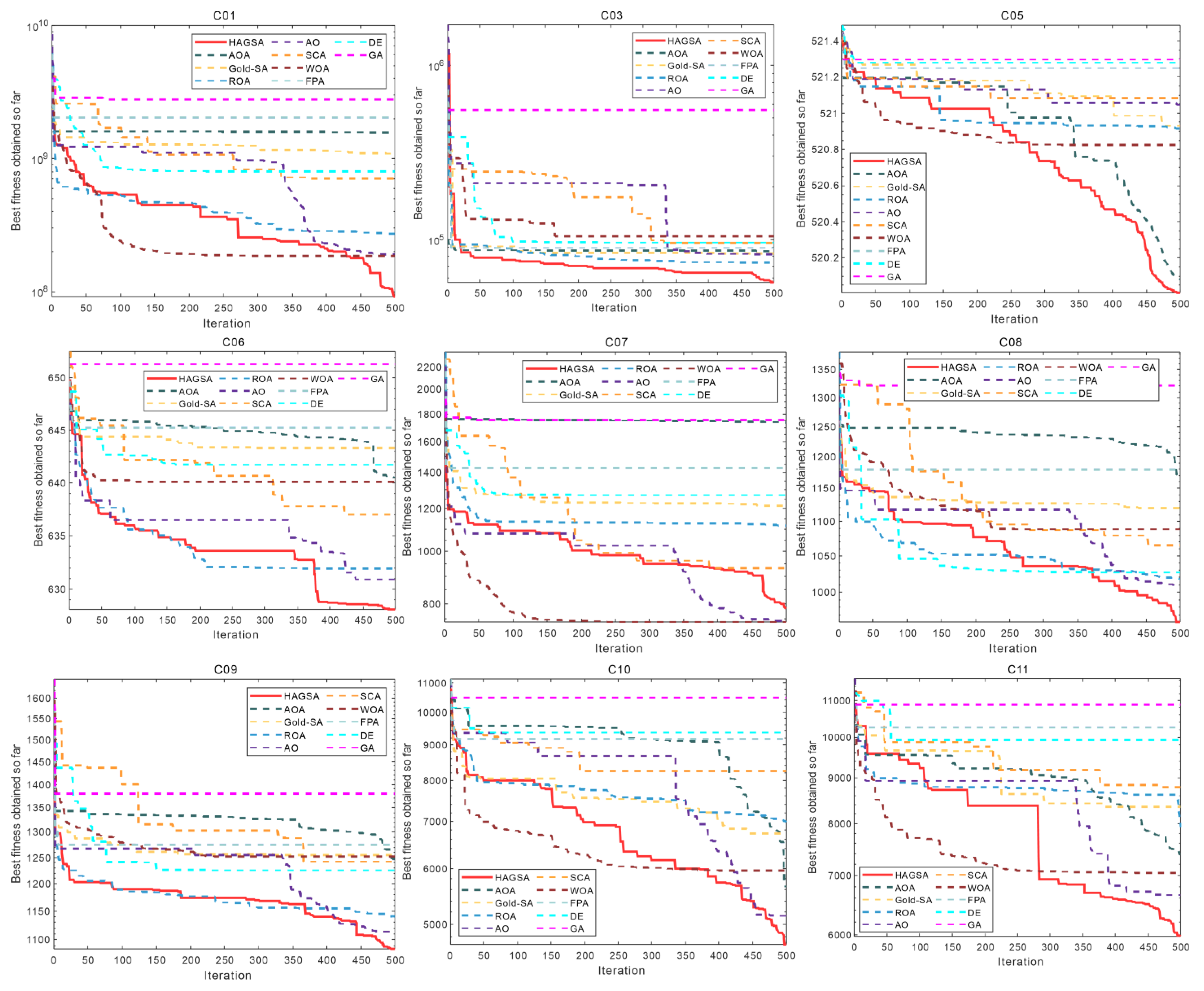
4.5. Convergence Behavior Analysis

In this subsection, we analyze the convergence behavior of each algorithm used over some benchmark functions. Figure 9 shows the convergence behavior of HAGSA, AOA, Gold-SA, ROA, AO, SCA, WOA, FPA, DE, and GA for selected functions. As can be seen from this figure, HAGSA achieves excellent behavior for most functions, which suggests the convergence of the proposed method. For unimodal functions (C01 and C03), although the convergence speed is slower than WOA in the early iteration (for C01), the convergence accuracy is higher than WOA at the end of the iteration. For C03, HAGSA has the fastest convergence speed and highest convergence accuracy. On the multimodal functions, HAGSA still maintains the fastest convergence speed and highest accuracy on most functions. In particular, for C05 and C06, although the global optimal is not found, HAGSA still has excellent performance compared to the others. However, the optimal value of HAGSA is ranked third and the WOA and AO are ranked first and second, respectively, when solving C07. For C10 and C11, it can be seen that the convergence curve of HAGSA is accelerated in the later stage of iteration; this is due to the excellent ability to jump out of the local optimal as a result of Brownian mutation. On hybrid functions, the convergence accuracy is still good compared to the others. For C16, C20, C21, and C22, the proposed HAGSA algorithm demonstrates its better performance compared to the original AOA and Gold-SA. On composition functions, the improvement is not obvious compared to the original Gold-SA and other well-known algorithms such as GA and FPA.

4.6. Wilcoxon Rank-Sum Test

Because the results obtained by each algorithm are random, in this subsection, we utilize the Wilcoxon rank-sum test (WRS) to evaluate the statistical significance difference between two samples at a significance level of 5% [2]. Specifically, if the p-value is less than 0.05, it indicates the statistical difference is significant; otherwise, the difference is not obvious. Furthermore, NaN denotes there is no difference between the two samples. The statistical results of the Wilcoxon rank-sum test are listed in Table 4; from this table, we can see that the proposed HAGSA algorithm shows better significant performance than the other algorithms on most benchmark functions.

4.7. Computational Time Analysis

To show the computational cost of the proposed HAGSA, in this subsection, we record the computational time cost obtained by algorithms on the CEC 2014 test suite. The statistical results are listed in Table 5; although HAGSA has the same computational complexity as AOA and Gold-SA, the computational time cost of HAGSA is more than that of AOA and Gold-SA. This is because HAGSA uses Brownian mutation to generate two candidates’ solutions to enhance the algorithm’s searchability and Levy flight is used to improve the exploitation ability of the hybrid algorithm. In addition, considering the NFL theorem, it is acceptable to increase computational time to obtain reliable solutions.

4.8. Industrial Engineering Design Problems

This subsection introduces five real-world industrial engineering design problems to evaluate the proposed algorithm’s searchability, including the car side crash design problem, pressure vessel design problem, tension spring design problem, speed reducer design problem, and cantilever beam design problem. Unlike benchmark functions, these industrial engineering design problems have many inequality and equality constraints, which is a vital challenge to MAs. In addition, using these problems helps evaluate the potential of algorithms to solve real-world problems.

4.8.1. Car Side Crash Design Problem

This problem aims to maintain the side impact crash performance and minimize the vehicle weight [48]. It has 11 parameters that need to be optimized; also, ten constraints were integrated into this problem. The model of this problem can be established as follows:
Consider x = [ x 1   x 2   x 3   x 4   x 5   x 6   x 7   x 8   x 9   x 10   x 11 ]
Minimize f ( x ) = Weight ,
Subject to { g 1 ( x ) = F a ( load   in   abdomen ) 1   kN , g 2 ( x ) = V × C u   ( dummy upper chest ) 0.32   m/s , g 3 ( x ) = V × C m   ( dummy middle chest ) 0.32   m/s , g 4 ( x ) = V × C l   ( dummy lower chest ) 0.32   m/s , g 5 ( x ) = Δ ur   ( upper rib deflection ) 32   mm , g 6 ( x ) = Δ mr   ( middle rib deflection ) 32   mm , g 7 ( x ) = Δ lr   ( lower rib deflection ) 32   mm , g 8 ( x ) = F   ( Public force ) p 4   kN , g 9 ( x ) = V MBP ( Velocity of   V Pillar at   middle point ) 9.9   mm/ms , g 10 ( x ) = V FD ( Velocity of front door at   V Pillar ) 15.7   mm/ms ,
Variable range { 0.5 x 1 x 7 1.5 ,   0.192 < x 8 , x 9 < 0.345 , 30 x 10 , x 11 30 ,
Table 6 shows the best results obtained by all algorithms. As shown in this table, the results of the proposed HAGSA are superior to those of other optimization techniques, and ROA and AO approaches are ranked second and third, respectively.

4.8.2. Pressure Vessel Design Problem

The pressure vessel design problem is shown in Figure 10. The goal of this problem is to minimize the total cost [49]. It has four design parameters: shell thickness (Ts), ball thickness (Th), shell radius (R), and shell length (L). The constraints and objective function can be expressed as follows:
Consider x = [ x 1   x 2   x 3   x 4 ] = [ T s   T h   R   L ]
Minimize f ( x ) = 0.6224 x 1 x 3 x 4 + 1.7781 x 2 x 3 2 + 3.1661 x 1 2 x 4 + 19.84 x 1 2 x 3
Subject to { g 1 ( x ) = x 1 + 0.0193 x 3 0 ,   g 2 ( x ) = x 3 + 0.00954 x 3 0 , g 3 ( x ) = π x 3 2 x 4 4 3 π x 3 3 + 1,296,000 0 ,   g 4 ( x ) = x 4 240 0
Variable range { 0 x 1 99 ,   0 x 2 99 , 10 x 3 200 ,   10 x 4 200
Figure 10. Pressure vessel design problem.
Mathematics 10 01567 g010
Table 7 shows the statistical results obtained by HAGSA and other comparison algorithms including AOA, Gold-SA, ROA, AO, SCA, WOA, FPA, DE, and GA. As can be seen from this table, HAGSA achieves competitive results in this design problem, and the results of ROA and AO are ranked second and third, respectively.

4.8.3. Tension Spring Design Problem

The main goal of this problem is to find the optimal parameters to minimize the production cost [50]. There are three parameters: wire diameter (d), mean diameter of the spring (D), and number of active coils (N), as shown in Figure 11. The mathematical model is expressed as follows:
Consider x = [ x 1   x 2   x 3 ] = [ d   D   N ]
Minimize f ( x ) = ( x 3 + 2 ) x 2 x 1 2
Subject to { g 1 ( x ) = 1 x 2 3 x 3 71,785 x 1 4 0 ,   g 2 ( x ) = 4 x 2 2 x 1 x 2 12,566 ( x 2 x 1 3 x 1 4 ) + 1 5108 x 1 2 0 , g 3 ( x ) = 1 140.45 x 1 x 2 2 x 3 0 ,   g 4 ( x ) = x 1 + x 2 1.5 1 0
Variable range { 0.05 x 1 2.00 ,   0.25 x 2 1.30 2.00 x 3 15.00
Figure 11. Tension spring design problem.
Mathematics 10 01567 g011
The statistical results of the tension spring design problem were obtained by HAGSA and other comparison algorithms as listed in Table 8. As can be seen from this table, the best cost of this design problem is 0.011196, and the three parameters are 0.050411, 0.37384, and 9.7854, respectively.

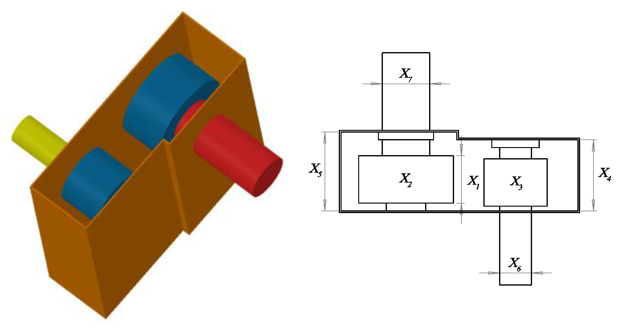
4.8.4. Speed Reducer Design Problem

This problem aims to construct a speed reducer with a minimum weight under constraints [51]. There are seven parameters: face width, the module of teeth, number of teeth in the pinion, length of the first shaft between bearings, length of the second shaft between bearings, the diameter of the first shafts, and the diameter of second shafts. Figure 12 shows the design of this problem, and its mathematical formula is as follows:
Consider x = [ x 1   x 2   x 3   x 4   x 5   x 6   x 7 ]
Minimize f ( x ) = 0.7854 x 1 x 2 2 ( 3.3333 x 3 2 + 14.9334 x 3 43.0934 ) 1.508 x 1 ( x 6 2 + x 7 2 ) + 7.4777 ( x 6 3 + x 7 3 ) ,
Subject to { g 1 ( x ) = 27 x 1 x 2 2 x 3 1 0 ,   g 2 ( x ) = 397.5 x 1 x 2 2 x 3 2 1 0 , g 3 ( x ) = 1.93 x 4 3 x 2 x 3 x 6 4 1 0 ,   g 4 ( x ) = 1.93 x 5 3 x 2 x 3 x 7 4 1 0 , g 5 ( x ) = ( 745 x 4 x 2 x 3 ) 2 + 16.9 × 10 6 110.0 x 6 3 1 0 ,   g 6 ( x ) = ( 745 x 4 x 2 x 3 ) 2 + 157.5 × 10 6 85.0 x 6 3 1 0 , g 7 ( x ) = x 2 x 3 40 1 0 ,   g 8 ( x ) = 5 x 2 x 1 1 0 , g 9 ( x ) = x 1 12 x 2 1 0 ,   g 10 ( x ) = 1.5 x 6 + 1.9 x 4 1 0 , g 11 ( x ) = 1.1 x 7 + 1.9 x 5 1 0 ,
Variable range { 2.6 x 1 3.6 ,   0.7 x 2 0.8 , 17 x 3 28 ,   7.3 x 4 8.3 , 7.8 x 5 8.3 ,   2.9 x 6 3.9 , 5.0 x 7 5.5
Figure 12. Speed reducer problem.
Mathematics 10 01567 g012
The proposed HAGSA is compared with AOA, Gold-SA, ROA, AO, SCA, WOA, FPA, DE, and GA. The statistical results are shown in Table 9. As can be seen, HAGSA is excellent for solving speed reducer design problems, and the results obtained by HAGSA are ranked first. The results of AOA and ROA are ranked second and third, respectively.

4.8.5. Cantilever Beam Design

The design of the cantilever beam is shown in Figure 13, and the goal of this problem is to minimize the total weight [52]. There are five parameters that need to be optimized. The objective function and constraints of this problem are as follows:
Consider x = [ x 1   x 2   x 3   x 4   x 5 ]
Minimize f ( x ) = 0.6224 ( x 1 + x 2 + x 3 + x 4 + x 5 )
Subject to g ( x ) = 60 x 1 3 + 27 x 2 3 + 19 x 3 3 + 7 x 4 3 + 1 x 5 3 1 0
Variable range 0.01 x 1 , x 2 , x 3 , x 4 , x 5 100
Figure 13. Cantilever beam structure.
Mathematics 10 01567 g013
The statistical results obtained by HAGSA, AOA, Gold-SA, ROA, AO, SCA, WOA, FPA, DE, and GA are shown in Table 10. From this table, HAGSA shows a lower cost than that of other optimization techniques, and the results of ROA and AO are ranked second and third, respectively.

5. Conclusions and Future Work

Considering the characteristic of AOA and Gold-SA, this paper proposes a hybrid optimization algorithm, namely HAGSA. First, Gold-SA is utilized to alleviate the shortcomings of AOA, such as low population diversity, premature convergence, and easy stagnation into local optimal solutions. Second, Levy flight and a new strategy called Brownian mutation are used to enhance the searchability of the hybrid algorithm.
We first used the CEC 2014 competition test suite to validate the optimization performance of HAGSA and its peers. The experimental results demonstrate that HAGSA outperforms other competitors in terms of optimization accuracy, convergence speed, robustness, and statistical difference. In addition, five industrial engineering design problems were carried out to test the ability of HAGSA to solve real-world problems. The experimental results also show that HAGSA is significantly better than its peers. Therefore, it is believed that HAGSA is a valuable method and can provide high-quality solutions to solve these kinds of problems. Although HAGSA has significant improvements over the original AOA and Gold-SA, its time consumption is a potential issue. This is because the BM strategy produces two candidate solutions and uses fitness evaluation to select the best solution. Thus, determining how to reduce the computational time under the premise of ensuring performance needs further research. In future works, we will: (1) improve the BM strategy to reduce the computational time without degrading HAGSA’s performance; (2) seek to hybridize other MAs to improve AOA’s optimization performance; and (3) apply HAGSA to solve combinatorial optimization problems (e.g., the traveling salesman problem, knapsack problem, and graph coloring problem). In addition, multilevel thresholding image segmentation would also be an interesting and meaningful research area.

Author Contributions

Q.L., Conceptualization, methodology, software, formal analysis, investigation, data curation, visualization, writing-original draft preparation, writing—review and editing, funding acquisition, validation, resources, project administration. N.L., supervision, writing-review and editing, resources, validation, funding acquisition. H.J., project administration, validation, conceptualization, supervision, methodology, writing—review and editing, funding acquisition. Q.Q., project administration, resources, supervision, validation, conceptualization, methodology, writing—review and editing, funding acquisition. L.A., writing—review and editing, supervision. Y.L., validation, writing—review and editing. All authors have read and agreed to the published version of the manuscript.

Funding

This research was funded by the Innovative Research Project for Graduate Students of Hainan Province under grant No. Qhys2021-190, the National Natural Science Foundation of China under grant No. 11861030, the Hainan Provincial Natural Science Foundation of China under grants No. 621RC511 and No. 2019RC176, the Natural Science Foundation of Fujian Province under grant No. 2021J011128, the Sanming University Introduces High Level Talents to Start Scientific Research Funding Support Project under grant No. 20YG14, and the Sanming University National Natural Science Foundation Breeding Project under grant No. PYT2105.

Institutional Review Board Statement

Not applicable.

Informed Consent Statement

Not applicable.

Data Availability Statement

The data presented in this study are available on request from the corresponding authors.

Acknowledgments

We acknowledge the anonymous reviewers for their constructive comments.

Conflicts of Interest

The authors declare no conflict of interest.

References

  1. Esparza, E.R.; Calzada, L.A.Z.; Oliva, D.; Heidari, A.A.; Zaldivar, D.; Cisneros, M.P.; Foong, L.K. An efficient harris hawks-inspired image segmentation method. Expert Syst. Appl. 2020, 155, 113428. [Google Scholar] [CrossRef]
  2. Liu, Q.; Li, N.; Jia, H.; Qi, Q.; Abualigah, L. Modified remora optimization algorithm for global optimization and multilevel thresholding image segmentation. Mathematics 2022, 10, 1014. [Google Scholar] [CrossRef]
  3. Ewees, A.A.; Abualigah, L.; Yousri, D.; Sahlol, A.T.; Al-qaness, A.A.; Alshathri, S.; Elaziz, M.A. Modified artificial ecosystem-based optimization for multilevel thresholding image segmentation. Mathematics 2021, 9, 2363. [Google Scholar] [CrossRef]
  4. Wang, S.; Liu, Q.; Liu, Y.; Jia, H.; Liu, L.; Zheng, R.; Wu, D. A hybrid SSA and SMA with mutation opposition-based learning for constrained engineering problems. Comput. Intell. Neurosci. 2021, 2021, 6379469. [Google Scholar] [CrossRef] [PubMed]
  5. Houssein, E.H.; Mahdy, M.A.; Blondin, M.J.; Shebl, D.; Mohamed, W.M. Hybrid slime mould algorithm with adaptive guided differential evolution algorithm for combinatorial and global optimization problems. Expert Syst. Appl. 2021, 174, 114689. [Google Scholar] [CrossRef]
  6. Wang, S.; Jia, H.; Liu, Q.; Zheng, R. An improved hybrid aquila optimizer and harris hawks optimization for global optimization. Math. Biosci. Eng. 2021, 18, 7076–7109. [Google Scholar] [CrossRef]
  7. Wu, D.; Wang, S.; Liu, Q.; Abualigah, L.; Jia, H. An Improved Teaching-Learning-Based Optimization Algorithm with Reinforcement Learning Strategy for Solving Optimization Problems. Comput. Intell. Neurosci. 2022, 2022, 1535957. [Google Scholar] [CrossRef]
  8. Zhang, H.; Wang, Z.; Chen, W.; Heidari, A.A.; Wang, M.; Zhao, X.; Liang, G.; Chen, H.; Zhang, X. Ensemble mutation-driven salp swarm algorithm with restart mechanism: Framework and fundamental analysis. Expert Syst. Appl. 2021, 165, 113897. [Google Scholar] [CrossRef]
  9. Giovanni, L.D.; Pezzella, F. An improved genetic algorithm for the distributed and flexible Job-shop scheduling problem. Eur. J. Oper. Res. 2010, 200, 395–408. [Google Scholar] [CrossRef]
  10. Wu, B.; Zhou, J.; Ji, X.; Yin, Y.; Shen, X. An ameliorated teaching–learning-based optimization algorithm based study of image segmentation for multilevel thresholding using Kapur’s entropy and Otsu’s between class variance. Inf. Sci. 2020, 533, 72–107. [Google Scholar] [CrossRef]
  11. Wang, S.; Jia, H.; Abualigah, L.; Liu, Q.; Zheng, R. An improved hybrid aquila optimizer and harris hawks algorithm for solving industrial engineering optimization problems. Processes 2021, 9, 1551. [Google Scholar] [CrossRef]
  12. Lin, S.; Jia, H.; Abualigah, L.; Altalhi, M. Enhanced slime mould algorithm for multilevel thresholding image segmentation using entropy measures. Entropy 2021, 23, 1700. [Google Scholar] [CrossRef] [PubMed]
  13. Su, H.; Zhao, D.; Yu, F.; Heidari, A.A.; Zhang, Y.; Chen, H.; Li, C.; Pan, J.; Quan, S. Horizontal and vertical search artificial bee colony for image segmentation of COVID-19 X-ray images. Comput. Biol. Med. 2021, 142, 105181. [Google Scholar] [CrossRef]
  14. Mirjalili, S.; Lewis, A. The whale optimization algorithm. Adv. Eng. Softw. 2016, 95, 51–67. [Google Scholar] [CrossRef]
  15. Khare, A.; Rangnekar, S. A review of particle swarm optimization and its applications in solar photovoltaic system. Appl. Soft Comput. 2013, 13, 2997–3006. [Google Scholar] [CrossRef]
  16. Mirjalili, S.; Mirjalili, S.M.; Lewis, A. Grey wolf optimizer. Adv. Eng. Softw. 2014, 69, 46–61. [Google Scholar] [CrossRef] [Green Version]
  17. Mirjalili, S.; Gandomi, A.H.; Mirjalili, S.Z.; Saremi, S.; Faris, H.; Mirjalili, S.M. Salp swarm algorithm: A bio-inspired optimizer for engineering design problems. Adv. Eng. Softw. 2017, 114, 163–191. [Google Scholar] [CrossRef]
  18. Mirjalili, S. The ant lion optimizer. Adv. Eng. Softw. 2015, 83, 80–98. [Google Scholar] [CrossRef]
  19. Mirjalili, S. Moth-flame optimization algorithm: A novel nature-inspired heuristic paradigm. Knowl. Based Syst. 2015, 89, 228–249. [Google Scholar] [CrossRef]
  20. Li, S.; Chen, H.; Wang, M.; Heidari, A.A.; Mirjalili, S. Slime mould algorithm: A new method for stochastic optimization. Future Gener. Comput. Syst. 2020, 111, 300–323. [Google Scholar] [CrossRef]
  21. Heidari, A.A.; Mirjalili, S.; Faris, H.; Aljarah, I.; Mafarja, M.; Chen, H. Harris hawks optimization: Algorithm and applications. Future Gener. Comput. Syst. 2019, 97, 849–872. [Google Scholar] [CrossRef]
  22. Abualigah, L.; Elaziz, M.A.; Sumari, P.; Geem, Z.; Gandomi, A.H. Reptile search algorithm (RSA): A nature-inspired meta-heuristic optimizer. Expert Syst. Appl. 2022, 191, 116158. [Google Scholar] [CrossRef]
  23. Abualigah, L.; Yousri, D.; Abd, E.M.; Ewees, A.A. Aquila optimizer: A novel meta-heuristic optimization algorithm. Comput. Ind. Eng. 2021, 157, 107250. [Google Scholar] [CrossRef]
  24. Mirjalili, S.; Mirjalili, S.M.; Hatamlou, A. Multi-verse optimizer: A nature-inspired algorithm for global optimization. Neural Comput. Appl. 2015, 27, 495–513. [Google Scholar] [CrossRef]
  25. Mirjalili, S. SCA: A sine cosine algorithm for solving optimization problems. Knowl. Based Syst. 2016, 96, 120–133. [Google Scholar] [CrossRef]
  26. Abualigah, L.; Diabat, A.; Mirjalili, S.; Elaziz, A.E.; Gandomi, A.H. The arithmetic optimization algorithm. Comput. Methods Appl. Mech. Eng. 2021, 376, 113609. [Google Scholar] [CrossRef]
  27. Tanyildizi, E.; Demir, G. Golden sine algorithm: A novel math-inspired algorithm. Golden sine algorithm: A novel math-inspired algorithm. Adv. Electr. Comput. Eng. 2017, 17, 71–78. [Google Scholar] [CrossRef]
  28. Neggaz, N.; Houssein, E.H.; Hussain, K. An efficient henry gas solubility optimization for feature selection. Expert Syst. Appl. 2020, 152, 113364. [Google Scholar] [CrossRef]
  29. Rashedi, E.; Nezamabadi-pour, H.; Saryazdi, S. GSA: A gravitational search algorithm. Inf. Sci. 2009, 179, 2232–2248. [Google Scholar] [CrossRef]
  30. Sun, P.; Liu, H.; Zhang, Y.; Meng, Q.; Tu, L.; Zhao, J. An improved atom search optimization with dynamic opposite learning and heterogeneous comprehensive learning. Appl. Soft Comput. 2021, 103, 107140. [Google Scholar] [CrossRef]
  31. Faramarzi, A.; Heidarinejad, M.; Stephens, B.; Mirjalili, S. Equilibrium optimizer: A novel optimization algorithm. Knowl.-Based Syst. 2021, 191, 105190. [Google Scholar] [CrossRef]
  32. Katoch, S.; Chauhan, S.S.; Kumar, V. A review on genetic algorithm: Past, present, and future. Multimed. Tools Appl. 2021, 80, 8091–8126. [Google Scholar] [CrossRef] [PubMed]
  33. Simon, D. Biogeography-based optimization. IEEE Trans. Evol. Comput. 2008, 12, 702–713. [Google Scholar] [CrossRef] [Green Version]
  34. Slowik, A.; Kwasnicka, H. Evolutionary algorithms and their applications to engineering problems. Neural Comput. Appl. 2020, 32, 12363–12379. [Google Scholar] [CrossRef] [Green Version]
  35. Hansen, N.; Ostermeier, A. Completely Derandomized Self-Adaptation in Evolution Strategies. Evol. Comput. 2001, 9, 159–195. [Google Scholar] [CrossRef]
  36. Wolpert, D.H.; Macready, W.G. No free lunch theorems for optimization. IEEE Trans. Evol. Comput. 1997, 1, 67–82. [Google Scholar] [CrossRef] [Green Version]
  37. Azizi, M.; Talatahari, S. Improved arithmetic optimization algorithm for design optimization of fuzzy controllers in steel building structures with nonlinear behavior considering near fault ground motion effects. Artif. Intell. Rev. 2021. [Google Scholar] [CrossRef]
  38. Agushaka, J.O.; Ezugwu, A.E. Advanced arithmetic optimization algorithm for solving mechanical engineering design problems. PLoS ONE 2021, 16, 0255703. [Google Scholar] [CrossRef]
  39. Wang, R.; Wang, W.; Xu, L.; Pan, J.; Chu, S. An adaptive parallel arithmetic optimization algorithm for robot path planning. J. Adv. Transport. 2021, 2021, 3606895. [Google Scholar] [CrossRef]
  40. Abualigah, L.; Diabat, A.; Sumari, P.; Gandomi, A.H. A novel evolutionary arithmetic optimization algorithm for multilevel thresholding segmentation of COVID-19 CT images. Processes 2021, 9, 1155. [Google Scholar] [CrossRef]
  41. Liu, Y.; Cao, B. A novel ant colony optimization algorithm with Levy flight. IEEE Access 2020, 8, 67205–67213. [Google Scholar] [CrossRef]
  42. Iacca, G.; Junior, V.C.S.; Melo, V.V. An improved jaya optimization algorithm with Levy flight. Expert Syst. Appl. 2021, 165, 113902. [Google Scholar] [CrossRef]
  43. Faramarzi, A.; Heidarinejad, M.; Mirjalili, S.; Gandomi, A.H. Marine Predators Algorithm: A nature-inspired metaheuristic. Expert Syst. Appl. 2020, 152, 113377. [Google Scholar] [CrossRef]
  44. Li, M.; Zhao, H.; Weng, X.; Han, T. A novel nature-inspired algorithm for optimization: Virus colony search. Adv. Eng. Softw. 2016, 92, 65–88. [Google Scholar] [CrossRef]
  45. Jia, H.; Peng, X.; Lang, C. Remora optimization algorithm. Expert Syst. Appl. 2021, 185, 115665. [Google Scholar] [CrossRef]
  46. Zhou, Y.; Wang, R.; Luo, Q. Elite opposition-based flower pollination algorithm. Neurocomputing 2016, 188, 294–310. [Google Scholar] [CrossRef]
  47. Ewees, A.A.; Elaziz, M.A.; Houssein, E.H. Improved grasshopper optimization algorithm using opposition-based learning. Expert Syst. Appl. 2018, 112, 156–172. [Google Scholar] [CrossRef]
  48. Yildiz, B.S.; Pholdee, N.; Bureerat, S.; Yildiz, A.R.; Sait, S.M. Enhanced grasshopper optimization algorithm using elite opposition-based learning for solving real-world engineering problems. Eng. Comput. 2021. [Google Scholar] [CrossRef]
  49. Houssein, E.H.; Helmy, B.E.; Rezk, H.; Nassef, A.M. An efficient orthogonal opposition-based learning slime mould algorithm for maximum power point tracking. Neural Comput. Appl. 2022, 34, 3671–3695. [Google Scholar] [CrossRef]
  50. Taheri, A.; Rahimizadeh, K.; Rao, R.V. An efficient balanced teaching-learning-based optimization algorithm with individual restarting strategy for solving global optimization problems. Inf. Sci. 2021, 576, 68–104. [Google Scholar] [CrossRef]
  51. Ahmadianfar, I.; Heidari, A.A.; Gandomi, A.H.; Chu, X.; Chen, H. RUN beyond the metaphor: An efficient optimization algorithm based on runge kutta method. Expert Syst. Appl. 2021, 181, 115079. [Google Scholar] [CrossRef]
  52. Cheng, Z.; Song, H.; Wang, J.; Zhang, H.; Chang, T.; Zhang, M. Hybrid firefly algorithm with grouping attraction for constrained optimization problem. Knowl. Based Syst. 2021, 220, 106937. [Google Scholar] [CrossRef]
Figure 1. Classification of MAs.
Mathematics 10 01567 g001
Figure 2. The different search phases of AOA.
Mathematics 10 01567 g002
Figure 3. Levy distribution and 2D Levy trajectory.
Mathematics 10 01567 g003
Figure 4. Brownian distribution and 2D Brownian trajectory.
Mathematics 10 01567 g004
Figure 5. Flowchart of HAGSA.
Mathematics 10 01567 g005
Figure 6. View of some CEC 2014 benchmark functions.
Mathematics 10 01567 g006
Figure 7. The radar graphs of algorithms on CEC 2014 benchmark functions.
Mathematics 10 01567 g007
Figure 8. Boxplot behavior of algorithms on some functions.
Mathematics 10 01567 g008aMathematics 10 01567 g008b
Figure 9. Convergence curve of algorithms on some functions.
Mathematics 10 01567 g009aMathematics 10 01567 g009b
Table 1. CEC 2014 benchmark functions.
Function TypesNo.Name of the FunctionDRangefmin
UnimodalC01Rotated High Conditioned Elliptic Function30[−100, 100]100
C02Rotated Bent Cigar Function30[−100, 100]200
C03Rotated Discus Function30[−100, 100]300
MultimodalC04Shifted and Rotated Rosenbrock Function30[−100, 100]400
C05Shifted and Rotated Ackley Function30[−100, 100]500
C06Shifted and Rotated Weierstrass Function30[−100, 100]600
C07Shifted and Rotated Griewank Function30[−100, 100]700
C08Shifted Rastrigin Function30[−100, 100]800
C09Shifted and Rotated Rastrigin Function30[−100, 100]900
C10Shifted Schwefel Function30[−100, 100]1000
C11Shifted and Rotated Schwefel Function30[−100, 100]1100
C12Shifted and Rotated Katsuura Function30[−100, 100]1200
C13Shifted and Rotated HappyCat Function30[−100, 100]1300
C14Shifted and Rotated HGBat Function30[−100, 100]1400
C15Shifted and Rotated Expanded Griewank plus Rosenbrock Function30[−100, 100]1500
HybridC16Shifted and Rotated Expanded Scaffer F6 Function30[−100, 100]1600
C17Hybrid Function 1(N = 3)30[−100, 100]1700
C18Hybrid Function 2(N = 3)30[−100, 100]1800
C19Hybrid Function 3(N = 4)30[−100, 100]1900
C20Hybrid Function 4(N = 4)30[−100, 100]2000
C21Hybrid Function 5(N = 5)30[−100, 100]2100
C22Hybrid Function 6(N = 5)30[−100, 100]2200
CompositionC23Composition Function 1(N = 5)30[−100, 100]2300
C24Composition Function 2(N = 3)30[−100, 100]2400
C25Composition Function 3(N = 3)30[−100, 100]2500
C26Composition Function 4(N = 5)30[−100, 100]2600
C27Composition Function 5(N = 5)30[−100, 100]2700
C28Composition Function 6(N = 5)30[−100, 100]2800
C29Composition Function 7(N = 3)30[−100, 100]2900
C30Composition Function 8(N = 3)30[−100, 100]3000
Table 3. The mean fitness and std obtained with the different algorithms on the CEC 2014 test suite.
FunctionHAGSAAOAGold-SAROAAOSCAWOAFPADEGA
C01Mean1.94 × 1081.08 × 1096.73 × 1083.59 × 1087.85 × 1085.11 × 1081.97 × 1094.63 × 1085.30 × 1092.77 × 109
Std7.50 × 1073.49 × 1082.21 × 1081.63 × 1083.92 × 1071.26 × 1083.25 × 1081.97 × 1082.23 × 1081.07 × 108
C02Mean2.40 × 10106.81 × 10106.18 × 10106.80 × 10106.83 × 10102.93 × 10108.59 × 10106.99 × 10105.09 × 10101.03 × 1011
Std7.78 × 1091.18 × 10109.47 × 1097.53 × 1091.27 × 1095.26 × 1097.45 × 1092.39 × 1091.02 × 10100.00
C03Mean8.55 × 1048.19 × 1048.73 × 1046.60 × 1048.72 × 1047.58 × 1049.20 × 1041.26 × 1057.01 × 1041.42 × 107
Std2.10 × 1036.52 × 1032.50 × 1037.55 × 1037.66 × 1031.61 × 1041.22 × 1046.25 × 1041.56 × 1041.25 × 104
C04Mean1.45 × 1041.05 × 1041.27 × 1042.54 × 1031.40 × 1042.57 × 1031.73 × 1041.74 × 1036.37 × 1032.58 × 104
Std7.37 × 1022.84 × 1033.47 × 1031.17 × 1031.95 × 1026.06 × 1022.18 × 1033.95 × 1022.59 × 1035.19 × 102
C05Mean5.20 × 1025.21 × 1025.21 × 1025.21 × 1025.21 × 1025.21 × 1025.21 × 1025.21 × 1025.21 × 1025.21 × 102
Std8.39 × 1028.06 × 1027.03 × 1021.07 × 10−18.92 × 10−27.53 × 10−28.15 × 10−28.17 × 10−26.61 × 10−28.05 × 10−2
C06Mean6.17 × 1026.38 × 1026.42 × 1026.35 × 1026.42 × 1026.39 × 1026.45 × 1026.39 × 1026.34 × 1026.50 × 102
Std3.562.452.423.072.761.971.432.822.632.05
C07Mean1.47 × 1031.34 × 1031.13 × 1039.16 × 1021.19 × 1039.50 × 1021.56 × 1037.41 × 1021.16 × 1031.75 × 103
Std7.04 × 101.06 × 1029.78 × 109.09 × 101.24 × 103. × 106.79 × 101.56 × 101.12 × 1027.10 × 10
C08Mean1.09 × 1031.14 × 1031.12 × 1031.13 × 1031.13 × 1031.19 × 1031.18 × 1031.13 × 1031.08 × 1031.31 × 103
Std2.42 × 103.04 × 103.10 × 102.57 × 102.02 × 102.22 × 101.37 × 104.63 × 102.32 × 102.23 × 10
C09Mean1.14 × 1031.22 × 1031.26 × 1031.37 × 1031.26 × 1031.22 × 1031.29 × 1031.20 × 1031.20 × 1031.38 × 103
Std1.65 × 102.17 × 102.71 × 102.23 × 101.89 × 102.49 × 101.67 × 105.07 × 102.70 × 102.31 × 10−13
C10Mean6.12 × 1037.26 × 1038.04 × 1036.34 × 1038.16 × 1037.97 × 1039.45 × 1036.57 × 1038.93 × 1031.07 × 104
Std6.25 × 1023.79 × 1025.47 × 1027.11 × 1025.84 × 1024.49 × 1023.61 × 1027.50 × 1022.87 × 1025.36 × 102
C11Mean7.56 × 1037.85 × 1038.90 × 1037.28 × 1037.81 × 1038.96 × 1031.01 × 1047.47 × 1039.31 × 1031.10 × 104
Std7.10 × 1024.20 × 1025.68 × 1026.88 × 1026.68 × 1022.55 × 1023.79 × 1027.89 × 1024.51 × 1024.69 × 102
C12Mean1.20 × 1031.20 × 1031.20 × 1031.20 × 1031.20 × 1031.20 × 1031.20 × 1031.20 × 1031.20 × 1031.21 × 103
Std5.52 × 105.78 × 10−15.35 × 10−15.62 × 10−15.98 × 10−15.89 × 10−16.48 × 10−16.75 × 10−15.80 × 10−19.19 × 10⁻¹
C13Mean1.30 × 1031.31 × 1031.31 × 1031.31 × 1031.31 × 1031.31 × 1031.31 × 1031.31 × 1031.31 × 1031.31 × 103
Std8.34 × 10−19.07 × 10−18.99 × 10−18.64 × 10−14.09 × 10−13.93 × 10−18.37 × 10−19.22 × 10−17.67 × 10−14.48 × 10⁻¹
C14Mean1.45 × 1031.63 × 1031.57 × 1031.47 × 1031.41 × 1031.49 × 1031.73 × 1031.42 × 1031.59 × 1031.79 × 103
Std1.44 × 104.41 × 104.36 × 102.20 × 105.87 × 101.99 × 102.46 × 109.003.95 × 103.58 × 10
C15Mean4.34 × 1032.50 × 1054.92 × 1049.04 × 1038.92 × 1042.54 × 1045.38 × 1054.74 × 1031.03 × 1059.16 × 105
Std2.25 × 1031.31 × 1053.55 × 1048.15 × 1033.54 × 101.62 × 1041.55 × 1052.24 × 1031.35 × 1054.74 × 10−10
C16Mean1.61 × 1031.61 × 1031.61 × 1031.61 × 1031.61 × 1031.61 × 1031.61 × 1031.61 × 1031.61 × 1031.61 × 103
Std3.71 × 10−13.70 × 10−13.21 × 10−14.71 × 10−14.08 × 10−11.95 × 10−12.08 × 10−14.66 × 10−12.37 × 10−11.88 × 10⁻¹
C17Mean8.59 × 1078.90 × 1071.36 × 1081.61 × 1071.64 × 1081.56 × 1072.47 × 1082.35 × 1079.17 × 1065.48 × 108
Std7.10 × 1066.17 × 1078.13 × 1071.40 × 1075.24 × 1065.76 × 1066.66 × 1072.13 × 1071.30 × 1072.33 × 108
C18Mean1.36 × 1072.44 × 1092.78 × 1092.90 × 1083.80 × 1094.77 × 1087.52 × 1096.11 × 1062.65 × 1081.20 × 1010
Std2.06 × 1072.04 × 1091.67 × 1096.85 × 1082.05 × 1062.52 × 1082.30 × 1097.19 × 1063.73 × 1083.82 × 109
C19Mean2.01 × 1032.24 × 1032.27 × 1032.30 × 1032.30 × 1032.25 × 1032.49 × 1032.32 × 1032.10 × 1032.80 × 103
Std5.12 × 101.05 × 1029.98 × 1019.65 × 103.15 × 103.29 × 107.58 × 105.24 × 106.27 × 102.51 × 10
C20Mean3.67 × 1041.86 × 1052.45 × 1059.06 × 1044.34 × 1055.90 × 1043.43 × 1064.97 × 1052.75 × 1041.07 × 108
Std3.96 × 1049.23 × 1041.27 × 1056.04 × 1045.11 × 1042.94 × 1044.51 × 1067.78 × 1052.08 × 1042.87 × 107
C21Mean1.12 × 1063.36 × 1075.47 × 1079.65 × 1065.65 × 1075.18 × 1061.07 × 1081.25 × 1075.17 × 1052.80 × 108
Std6.21 × 1052.39 × 1072.92 × 1079.83 × 1061.66 × 1062.86 × 1065.82 × 1079.65 × 1067.13 × 1052.14 × 108
C22Mean2.85 × 1034.93 × 1034.69 × 1033.28 × 1036.49 × 1033.37 × 1033.08 × 1043.32 × 1033.08 × 1031.68 × 105
Std2.12 × 1022.12 × 1071.78 × 1037.41 × 1022.78 × 1021.72 × 1023.05 × 1042.89 × 1022.52 × 1027.01 × 104
C23Mean2.50 × 1032.50 × 1032.50 × 1032.50 × 1032.50 × 1032.72 × 1032.50 × 1032.72 × 1032.84 × 1032.50 × 103
Std0.000.000.000.000.003.17 × 100.004.01 × 109.01 × 100.00
C24Mean2.60 × 1032.60 × 1032.60 × 1032.60 × 1032.60 × 1032.63 × 1032.60 × 1032.61 × 1032.69 × 1032.60 × 103
Std0.008.87 × 10−20.001.46 × 10−72.34 × 10−51.87 × 100.005.811.34 × 100.00
C25Mean2.70 × 1032.70 × 1032.70 × 1032.70 × 1032.70 × 1032.75 × 1032.70 × 1032.72 × 1032.73 × 1032.70 × 103
Std0.000.000.000.000.001.15 × 100.001.83 × 108.740.00
C26Mean2.77 × 1032.77 × 1032.77 × 1032.77 × 1032.78 × 1032.70 × 1032.79 × 1032.74 × 1032.73 × 1032.79 × 103
Std4.33 × 104.41 × 104.25 × 104.62 × 104.99 × 104.96 × 10−12.35 × 1018.00 × 104.33 × 102.39 × 10
C27Mean2.90 × 103 4.05 × 1032.90 × 1032.90 × 1032.90 × 1033.91 × 1032.90 × 1033.99 × 103.86 × 1032.90 × 103
Std0.003.71 × 1020.000.003.982.65 × 1020.002.42 × 1022.46 × 1020.00
C28Mean3.00 × 1035.34 × 1033.00 × 1033.00 × 1033.00 × 1035.95 × 1033.00 × 1035.40 × 1035.36 × 1033.00 × 103
Std0.002.75 × 1030.000.000.006.11 × 1020.008.95 × 1024.64 × 1020.00
C29Mean3.10 × 1034.32 × 1083.10 × 1037.17 × 1061.46 × 1044.43 × 1073.10 × 1031.79 × 1076.87 × 1073.10 × 103
Std0.001.80 × 1080.007.00 × 1066.28 × 1041.75 × 1070.001.63 × 1075.50 × 1070.00
C30Mean3.20 × 1034.16 × 1063.20 × 1033.29 × 1051.66 × 1056.97 × 1053.20 × 1034.02 × 1054.17 × 1053.20 × 103
Std0.002.65 × 1060.002.80 × 1051.44 × 1052.87 × 1050.002.76 × 1052.34 × 1050.00
Table 4. Statistical results of Wilcoxon rank-sum test obtained by each algorithm.
FunctionHAGSA vs.
AOAGold-SAROAAOSCAWOAFPADEGA
C013.02 × 10−113.02 × 10−112.71 × 10−22.13 × 10−44.08 × 10−112.64 × 10−13.02 × 10−111.29 × 10−92.37 × 10−12
C023.02 × 10−113.02 × 10−117.01 × 10−23.02 × 10−115.83 × 10−133.02 × 10−113.02 × 10−113.02 × 10−111.21 × 10⁻¹²
C033.02 × 10−113.02 × 10−113.32 × 10−62.49 × 10−62.00 × 10−56.52 × 10−93.02 × 10−113.82 × 10−103.02 × 10⁻¹¹
C043.02 × 10−113.02 × 10−112.06 × 10−22.61 × 10−104.71 × 10−41.31 × 10−83.02 × 10−113.69 × 10−111.21 × 10⁻¹²
C051.78 × 10−103.02 × 10−113.02 × 10−113.02 × 10−113.02 × 10−113.02 × 10−113.02 × 10−113.02 × 10−113.02 × 10⁻¹¹
C064.62 × 10−103.02 × 10−112.75 × 10−37.73 × 10−22.23 × 10−91.29 × 10−113.02 × 10−111.30 × 10−12.95 × 10−11
C073.02 × 10−116.07 × 10−111.45 × 10−13.02 × 10−112.13 × 10−53.02 × 10−113.02 × 10−113.02 × 10−113.16 × 10⁻¹²
C083.02 × 10−113.02 × 10−111.73 × 10−61.25 × 10−73.02 × 10−112.84 × 10−43.02 × 10−115.49 × 10−119.40 × 10⁻¹²
C093.02 × 10−113.02 × 10−111.44 × 10−27.70 × 10−83.34 × 10−114.42 × 10−63.02 × 10−116.12 × 10−101.21 × 10⁻¹²
C102.23 × 10−93.02 × 10−115.09 × 10−82.97 × 10−13.02 × 10−111.46 × 10−103.02 × 10−113.02 × 10−113.02 × 10⁻¹¹
C113.50 × 10−93.02 × 10−111.37 × 10−35.01 × 10−13.34 × 10−112.96 × 10−53.02 × 10−113.02 × 10−113.02 × 10⁻¹¹
C126.91 × 10−42.39 × 10−81.76 × 10−22.90 × 10−11.69 × 10−95.27 × 10−54.50 × 10−113.02 × 10−112.80 × 10⁻¹¹
C133.02 × 10−113.69 × 10−111.38 × 10−26.07 × 10−111.68 × 10−33.02 × 10−113.02 × 10−113.02 × 10−117.88 × 10⁻¹²
C143.02 × 10−113.02 × 10−114.22 × 10−41.33 × 10−101.39 × 10−61.09 × 10−103.02 × 10−113.02 × 10−111.72 × 10⁻¹²
C153.02 × 10−113.02 × 10−115.49 × 10−13.02 × 10−111.69 × 10−92.37 × 10−103.02 × 10−113.02 × 10−111.21 × 10⁻¹²
C161.56 × 10−84.18 × 10−91.64 × 10−52.23 × 10−94.50 × 10−113.20 × 10−93.02 × 10−113.02 × 10−113.02 × 10⁻¹¹
C173.02 × 10−113.02 × 10−116.97 × 10−33.95 × 10−17.22 × 10−62.43 × 10−53.02 × 10−112.32 × 10−23.00 × 10−11
C183.02 × 10−113.02 × 10−114.86 × 10−31.21 × 10−106.70 × 10−113.96 × 10−83.02 × 10−114.08 × 10−112.63 × 10⁻¹¹
C193.02 × 10−113.34 × 10−112.39 × 10−44.35 × 10−55.61 × 10−53.55 × 10−13.02 × 10−114.57 × 10−91.72 × 10−12
C203.02 × 10−111.41 × 10−91.00 × 10−39.83 × 10−81.91 × 10−22.20 × 10−73.69 × 10−117.96 × 10−33.02 × 10−11
C213.02 × 10−113.02 × 10−113.18 × 10−44.17 × 10−22.28 × 10−51.07 × 10−73.02 × 10−113.38 × 10−23.02 × 10−11
C225.49 × 10−111.46 × 10−105.32 × 10−33.03 × 10−27.70 × 10−81.64 × 10−53.02 × 10−114.06 × 10−23.02 × 10−11
C231.21 × 10−12NaNNaNNaN1.21 × 10−121.21 × 10⁻¹²NaN1.21 × 10−12NaN
C241.21 × 10−12NaN1.61 × 10−16.62 × 10−41.21 × 10−121.21 × 10⁻¹²NaN1.21 × 10−12NaN
C251.21 × 10−12NaNNaNNaN1.21 × 10−121.93 × 10⁻⁹NaN1.21 × 10−12NaN
C268.11 × 10−83.55 × 10−12.86 × 10−44.56 × 10−23.98 × 10−69.59 × 10−98.00 × 10−17.40 × 10−31.89E-02
C271.21 × 10−12NaNNaN4.19 × 10−21.21 × 10−121.21 × 10⁻¹²NaN1.21 × 10−12NaN
C281.21 × 10−12NaNNaNNaN1.21 × 10−121.21 × 10⁻¹²NaN1.21 × 10−12NaN
C291.21 × 10−12NaN6.61 × 10−51.61 × 10−11.21 × 10−121.21 × 10⁻¹²NaN1.21 × 10−12NaN
C301.21 × 10−12NaN6.25 × 10−101.31 × 10−71.21 × 10−121.21 × 10⁻¹²NaN1.21 × 10−12NaN
Table 5. The computational time for HAGSA and its peers.
FunctionHAGSAAOAGold-SAROAAOSCAWOAFPADEGA
C010.53750.17220.12600.35870.33030.17560.14820.21020.27430.1516
C020.59980.14870.09180.29180.28540.14910.13320.16970.20100.1048
C030.55190.16590.10940.23950.28170.15880.13910.15580.20500.1043
C040.50850.15850.09290.25450.24990.14900.18030.14720.19710.1027
C050.59590.15640.13340.36150.34040.15210.17940.17050.23650.1136
C066.72341.12441.49285.55712.38891.52031.58371.56703.12401.3135
C070.64730.16050.12030.28720.32830.18500.11920.16610.22900.1047
C080.47860.14470.10270.29720.24930.13910.12120.17070.17990.1051
C090.60480.18470.10610.30450.27350.16810.12890.17910.21010.1046
C100.82560.19800.14400.42170.43600.20120.14740.20880.33060.1520
C110.89860.21000.15960.74390.40110.21260.18020.21470.35690.2055
C121.27240.32450.26021.12080.61990.32060.29460.32600.73700.3250
C130.53310.14510.09330.25550.29300.15410.11370.15410.20130.0944
C140.51300.15080.11080.30540.28160.19560.11800.15090.18550.1184
C150.49460.16100.13200.33720.30800.19140.14210.17710.22450.1277
C160.50780.15380.09780.32740.31630.15990.11640.19520.23970.1200
C170.60810.16840.15370.42100.32020.17300.18520.17900.28570.1479
C180.48030.14390.10280.31620.33320.25050.11380.20670.21150.1057
C191.67770.34500.31211.26460.70300.51360.31950.54900.85680.2681
C200.49750.15840.09870.31220.32950.15770.13710.19580.21950.1226
C210.58460.20160.12690.43380.32110.17940.15870.17440.27010.1310
C220.67560.19510.13080.58800.36880.19320.15340.20290.31520.1749
C231.88110.36950.31461.35980.75760.36920.41630.39300.92360.3200
C241.45120.29160.24591.12420.59350.42640.27250.41990.94950.2777
C251.63960.33340.28781.31090.70710.34650.31060.45181.03070.3435
C266.48001.52582.09845.04023.02122.02101.77591.73844.37101.6796
C276.33081.53341.28724.73502.86451.86171.84531.75054.31881.5384
C281.75700.46840.39551.11510.84010.45850.53620.66381.12720.3811
C292.07520.49420.62051.52710.95430.72520.63150.63431.42550.6466
C301.23670.33210.27590.89860.66840.34310.31480.35810.79410.4417
Table 6. Statistical results of car side crash design problem.
AlgorithmOptimum VariablesOptimum Cost
x1x2x3x4x5x6x7x8x9x10x11
HAGSA0.51.2530.51.1090.50.50.5010.3440.1923.9046.38122.9765
AOA0.51.2620.51.1560.50.7720.50.3100.1920.3651.16223.2139
Gold-SA0.51.2780.6121.1020.5441.3230.50.3450.3450.1700.29423.9711
ROA0.51.2350.51.1660.51.1100.50.3410.1920.2752.92623.0801
AO0.7241.1750.5021.2000.50.7920.50.3080.1920.7392.83723.1694
SCA0.5671.3340.5401.1670.51.1090.50.2330.2630.3012.39324.3513
WOA0.9531.1060.51.2060.5240.5590.5010.2820.2980.2467.32624.6495
FPA0.5321.3220.5151.1430.6160.5160.5340.1970.1970.7101.89224.1309
DE0.5051.4460.5211.1820.51.4660.50.3120.1921.00813.26624.7181
GA1.0731.04650.5951.0960.7140.5020.5210.3220.2645.5498.21525.4504
Table 7. Statistical results of the pressure vessel design problem.
AlgorithmOptimum VariablesOptimum Cost
TsThRL
HAGSA0.83047950.377066444.00935154.95575982.8355
AOA0.83954750.411384544.27936156.88836068.3284
Gold-SA0.71401790.461943540.49522197.73626090.4062
ROA0.86100260.393498444.96907144.29216023.0145
AO0.80300470.452448643.65139158.31466024.2153
SCA0.9630870.47693951.441287.30956246.7789
WOA0.9377260.47337349.943698.81346195.7655
FPA0.9718430.47840252.547981.32256393.2109
DE1.0096770.49883454.047069.22706398.6641
GA1.0254220.48403754.745864.67206439.9228
Table 8. Statistical results of the tension spring design problem.
AlgorithmOptimum VariablesOptimum Cost
dDN
HAGSA0.0504110.373849.78540.011196
AOA0.0517910.3889.55560.012026
Gold-SA0.0606830.679823.10630.012783
ROA0.0592210.63083.51880.012209
AO0.050.33719313.09050.012721
SCA0.0613650.703552.92320.013043
WOA0.05020690.35122412.3360.012692
FPA0.101871.0939.53870.130890
DE0.067660.9079352.08710.016985
GA0.054010.4651139.67970.015848
Table 9. Statistical results of the speed reducer design problem.
AlgorithmOptimum VariablesOptimum Cost
x1x2x3x4x5x6x7
HAGSA3.497670.7177.37.80013.349825.285592995.4897
AOA3.507760.7177.776857.961333.350755.285573007.0806
Gold-SA3.494410.7177.37.83.423835.28723016.2163
ROA3.507760.7177.776857.961333.350755.285573007.0806
AO3.497480.7178.076457.83.351625.285733002.8462
SCA3.60.7178.38.33.430325.300133085.2732
WOA3.52470.7178.144418.058973.350915.285683019.883
FPA3.60.7177.37.83.412615.281433056.8032
DE3.51190.7178.38.33.373565.381513088.6759
GA3.48960.7177.713887.83.656145.292183094.3185
Table 10. Statistical results of the cantilever beam design problem.
AlgorithmOptimum VariablesOptimum Cost
x1x2x3x4x5
HAGSA5.92715.39624.50813.4762.17261.3404
AOA6.47465.5154.11383.78271.87241.3577
Gold-SA5.79085.01424.93973.41752.57131.3562
ROA5.85675.43164.43423.65422.12631.3418
AO5.82195.45724.45513.55172.21981.342
SCA5.7815.56694.99923.50492.50941.3954
WOA6.64245.01844.84513.04282.2871.3626
FPA5.77636.42394.69383.65011.66851.3861
DE7.13234.96124.25593.37482.57971.3918
GA6.51954.19435.76434.18472.28621.4320
Publisher’s Note: MDPI stays neutral with regard to jurisdictional claims in published maps and institutional affiliations.

