The Trefoil Soliton

Abstract

The Kiepert trefoil is an algebraic curve with remarkable geometric and number theoretic properties. Ludwig Kiepert, generalizing ideas due to Serret and Liouville, determined that it could be parametrized by arc length in terms of elliptic functions. In this note, we observe some other properties of the curve. In particular, the curve is a special example of a buckled ring, and thus a solitary wave solution to the planar filament equation, evolving by rotation. It is also a solitary wave solution to a flow in the (three-dimensional) filament hierarchy, evolving by translation.

1. Introduction

The problem of finding curves whose arc length can be expressed as an elliptic integral of the first kind inspired many nineteenth century mathematicians. A. Legendre [1] saw that the Bernoulli Lemniscate, $r^2=2cos(2\theta )$, had this property, which was already known by Fagnano, and sought other examples. J. Serret constructed a family of such curves [2], and J. Liouville extended Serret’s results [3]. See [4], pp. 727, 733–739, for a readable account of Liouville’s work.

In 1870, Friedrich Wilhelm A. L. Kiepert extended the family of such curves [5]. Among the curves he found was the curve referred to here as the Kiepert trefoil, given by the polar equation $r^3=2cos(3\theta )$ (or more generally, $r^3={\alpha }^{3}cos(3\theta )$). It is an algebraic curve of genus 1. Its arc length parametrization is given by certain elliptic functions known as Dixon functions [6]. The curve possesses many remarkable geometric and number theoretic properties; some of them can be found in [6,7,8,9,10].

In this note, we will focus on the Kiepert trefoil as solution to two variational problems. For the first, we will see that it evolves by pure rotation under the planar filament flow. For the other, the trefoil can be characterized as the only closed curve except for the circle that evolves under the flow by translation in the binormal direction (Theorem 1).

2. The Filament Equation

The vortex filament equation is an equation for the evolution of curves given by

$$\frac{\partial \gamma }{\partial t}={\gamma }_t=I_1=\kappa B$$

(1)

where $s\to \gamma (t,s)$ is an arc-length parametrized curve evolving in time t, $\kappa =\kappa (t,s)$ is the curvature, $\tau =\tau (t,s)$ is the torsion and $\{T,N,B\}$ is the orthonormal Frenet frame. The Frenet equations are

$${\gamma }_s=T{T}_s=\kappa N,N_s=-\kappa T+\tau B,B_s=-\tau N.$$

If the initial curve $\gamma (0,s)$ is an elastic curve, then under (1) $\gamma$ evolves by rigid motion. It is a solitary wave solution or soliton. The elastic curves are the critical points of the variational problem

$${\mathcal{F}}_{\lambda }(\gamma )=\int {\kappa }^2+\lambda ds,$$

where $\lambda$ is a Lagrange multiplier acting as a length constraint. The solutions with $\lambda =0$ are the free elastic curves (see [11] for details.)

Equation (1) is just the first of an infinite hierarchy of commuting flows, determined by vector fields $I_n$, which correspond under the Hasimoto transformation to the nonlinear Schrödinger Equation (NLS). (See [12,13].) We will consider the next two flows. They are

$${\gamma }_t=I_2=\frac{1}{2}{\kappa }^{2}T+{\kappa }_{s}N+\kappa \tau B$$

(2)

and

$${\gamma }_t=I_3={\kappa }^2\tau T+(2{\kappa }_s\tau +\kappa {\tau }_s)N+(\kappa {\tau }^2-{\kappa }_{ss}-\frac{1}{2}{\kappa }^3)B.$$

(3)

Critical points for $\int \frac{1}{2}{\kappa }^2\tau ds$ are soliton solutions to the flow $\mathcal{G}$ given by (2); critical points for $\int \frac{1}{2}{({\kappa }_s)}^2+\frac{1}{2}{\kappa }^2{\tau }^2-\frac{1}{8}{\kappa }^{4}ds$ are soliton solutions for the flow $\mathcal{H}$ given by (3).

3. The Second Flow

The flow $\mathcal{G}$ defined by Equation (2) has the nice property that initial curves with no torsion (i.e., planar curves) remain planar under the evolution. This happens for alternate terms in the hierarchy and allows one to consider the planar filament equation (see, e.g., [14]).

Buckled rings are equilibrium configurations of closed elastic rings under uniform pressure. They are solitons of the planar filament equation (see [12,14]); that is, they evolve by isometries and parameter shift under the flow. Buckled rings are closed (i.e., periodic) solutions of the differential equation

$${\kappa }_{ss}+\frac{1}{2}{\kappa }^3+\lambda \kappa =p$$

where $\lambda$ is a Lagrange multiplier corresponding to a length constraint and p is the pressure. The quantity p may also be viewed as a Lagrange multiplier corresponding to a constraint on the area. Integrating,

$${({\kappa }_s)}^2+\frac{1}{4}{\kappa }^4+\lambda {\kappa }^2-2p\kappa =c.$$

(4)

Various authors have given explicit solutions to the buckled ring problem, from early work by Greenhill [15] to the recent work of Djondjorov et al. [16]. The most challenging detail concerns the condition for a solution to be a closed curve.

The fact that the Kiepert trefoil is a solution to the buckled ring problem was noted by Greenhill ([15] p. 477), but seems to have been forgotten until recently. Wegner mentions it in a recent paper [17]. The curvature of the trefoil $r^3={\alpha }^{3}cos(3\theta )$ satisfies the differential equation

$${({\kappa }_s)}^2+\frac{1}{4}{\kappa }^4=AkA=\frac{16}{{\alpha }^3}$$

(5)

The solution to this equation can be expressed very simply as a multiple of the reciprocal of a Weierstrass ℘-function $\wp (s;0,g_3)$ corresponding to the hexagonal lattice. Exploiting this fact, we can embed the trefoil within a family of solutions defined as follows: The Weierstrass function $\wp (z;g_2,g_3)$ is the elliptic function satisfying the differential equation

$${\wp }^{\prime }{(z)}^2=4\wp {(z)}^3-g_2\wp (z)-g_3$$

(6)

Proposition 1.

Given a and b, let $g_2=ab$ and $g_3=a^2/4$. Then $\kappa (s)=\frac{a}{\wp (s;g_2,g_3)}+b$ is a solution to Equation (4) for $\lambda =-\frac{3}{2}{b}^2$, $p=2a-b^3$, and $c=(\frac{3}{4}{b}^4-4ab)$.

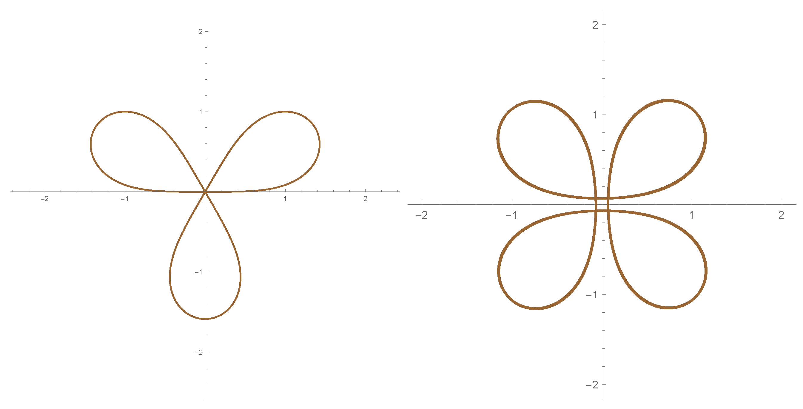
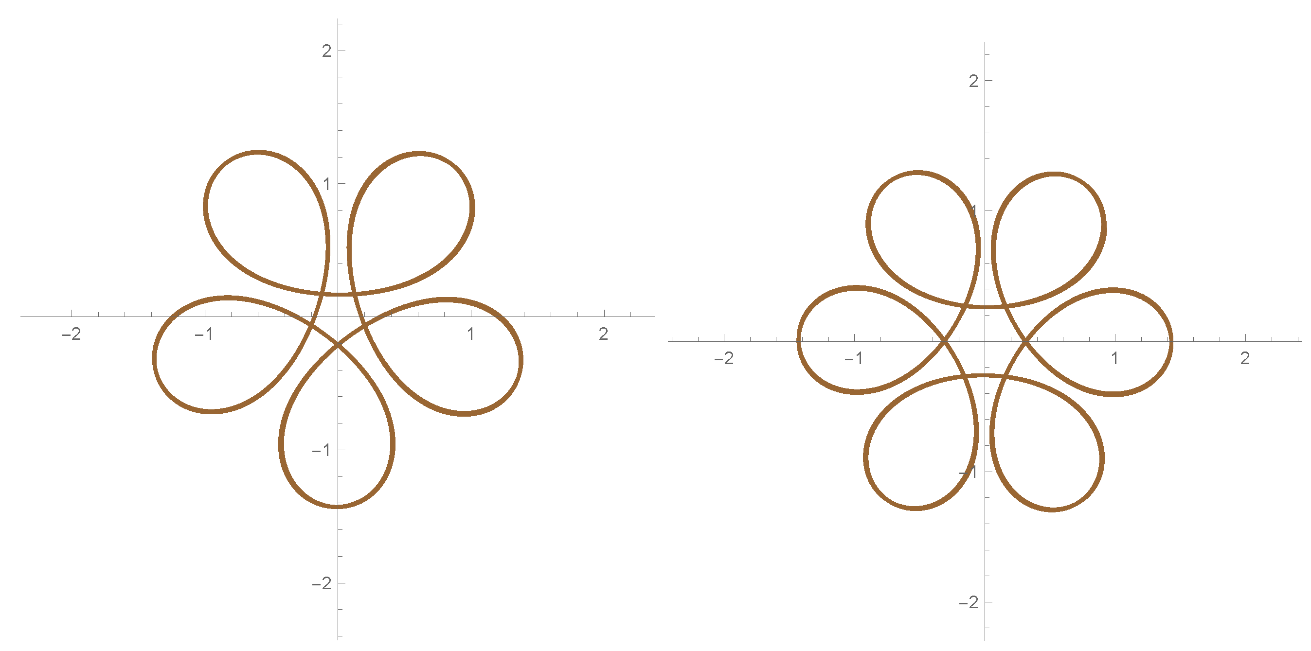
For convenience assume $p=2$. This is accomplished by setting $a=b^3/2+1$. As b varies we have a one-parameter family of solutions to Equation (4), infinitely many of which are buckled rings. (Figure 1, Figure 2 and Figure 3). For $b=0$, the curve is the trefoil $r^3=4cos(3\theta )$. Note that the trefoil is a special solution: $\lambda =0$. By analogy with the free elastic curve, one can say that the trefoil is a free buckled ring. In particular, the Kiepert trefoil evolves by a pure rotation. The vector field $I_2=\frac{1}{2}{\kappa }^{2}T+{\kappa }_{s}N$ along the trefoil is a Killing field, the restriction of an infinitestimal isometry of the plane (see, e.g., [13,14]).

4. The Third Flow

Now we consider the evolution Equation (3); ${\gamma }_t=I_3$. Unlike the previous example, planar solutions need not remain planar under the flow. Restricting attention to planar solutions, the Euler–Lagrange equation for critical points of $\mathcal{H}$ is

$$E={\kappa }_{ssss}+\frac{5}{2}{\kappa }^2{\kappa }_{ss}+\frac{5}{2}\kappa {\kappa }_s^2+\frac{3}{8}{\kappa }^5=0.$$

(7)

Since this corresponds to a completely integrable finite-dimensional Hamiltonian system, the solutions of this equation should in theory be determined by quadratures, and indeed there are sufficiently many first integrals in involution. From the general theory (see [18] for details), there are two important vector fields defined along a solution curve. The vector field

$$J=\left(-\frac{3}{8}{\kappa }^4+\frac{1}{2}{\kappa }_s^2-\kappa {\kappa }_{ss}\right)T+\left(-{\kappa }_{sss}-\frac{3}{2}{\kappa }^2{\kappa }_s\right)N$$

is constant along solutions. The vector field $I_3=(-{\kappa }_{ss}-\frac{1}{2}{\kappa }^3)B$ satisfies the equation

$$T\times J={(I_3)}_s$$

(8)

As shown in [18], the vector fields $I_3$ and J determine a cylindrical coordinate system and allow one to solve the Frenet equations once the curvature $\kappa$ is determined.

In [8], the authors consider special solutions to Equation (7) satisfying the equation

$${({\kappa }_s)}^2+\frac{1}{4}{\kappa }^4=P(\kappa )$$

where $P(\kappa )$ is a polynomial. Note that buckled rings all satisfy such an equation. They establish that the only polynomials are $P_1(\kappa )=a{\kappa }^2+4a^2$ and $P_2(\kappa )=b\kappa$.

The solutions using $P_1$ (up to scaling) are two specific (non-closed) elastic curves with curvature

$$\kappa =A\mathrm{cn}(\alpha s,p)A=2\alpha p$$

where the elliptic modulus is

$$p^2=\frac{3-\sqrt{3}}{6}\mathrm{or}{p}^2=\frac{3+\sqrt{3}}{6}.$$

For the polynomial $P_2$, the only solutions (up to scaling) are the Kiepert trefoil and the cirle (if $b\ne 0$) and the line ($b=0$). In particular, the trefoil is the only buckled ring satisfying Equation (7).

In fact, for the trefoil the vector field J vanishes. Consequently, Equation (8) implies that $I_3$ is a constant vector field. Conversely, for planar curves, if $I_3$ is constant then $J=0$.

The Hamiltonian flow for this member of the hierarchy is ${\gamma }_t=I_3$. Thus we can conclude:

Theorem 1.

The Kiepert trefoil and the circle are the only closed curves that evolve by translation under the flow (3).

References

- Legendre, A. Traité des Fonctions Elliptiques; Imprimerie de Huzard-Courcier: Paris, France, 1925; Volume I. [Google Scholar]
- Serret, J.-A. Mémoire sur la représentation géométrique des fonctions elliptiques et ultra-elliptiques. J. Math. Pures Appl. 1845, 10, 257–285. [Google Scholar]
- Liouville, J. Sur la division du périmètre de la lemniscate, le diviseur étant un nombre entier réel ou complexe quelconque. C. R. 1843, 17, 635–640. [Google Scholar]
- Lutzen, J. Joseph Liouville 1809–1882: Master of Pure and Applied Mathematics; Studies in the History of Mathematics and the Physical Sciences; Springer: Berlin/Heidelberg, Germany, 1990. [Google Scholar]
- Kiepert, L. De Curvis Quarum Arcus Integralibus Ellipticis Primi Generis Exprimuntur; Friedrich-Wilhelms-Universität: Berlin, Germany, 1870. [Google Scholar]
- Langer, J.; Singer, D. The Trefoil. Milan J. Math. 2014, 82, 161–182. [Google Scholar] [CrossRef]
- Clark, T. The Trefoil: An Analysis in Curve Minimization and Spline Theory. Ph.D. Thesis, Case Western Reserve Universiy, Cleveland, OH, USA, 2020. Available online: http://rave.ohiolink.edu/etdc/view?acc_num=case1596460534956624 (accessed on 2 January 2022).
- Clark, T.A.; Singer, D.A. The Trefoil Spline. Comput. Aided Des. 2022; in press. [Google Scholar] [CrossRef]
- Langer, J.; Singer, D. Subdividing the Trefoil by Origami. Geometry 2013, 2013, 171–180. [Google Scholar] [CrossRef]
- Zwikker, C. The Advanced Geometry of Plane Curves and Their Applications; Dover Publications: Mineola, NY, USA, 1963. [Google Scholar]
- Langer, J.; Singer, D. On the total squared curvature of closed curves. J. Differ. Geom. 1984, 20, 1–22. [Google Scholar] [CrossRef]
- Hasimoto, H. A soliton on a vortex filament. J. Fluid Mech. 1972, 51, 477–485. [Google Scholar] [CrossRef]
- Langer, J.; Perline, R. Poisson Geometry of the Filament Equation. J. Nonlinear Sci. 1991, 1, 71–83. [Google Scholar] [CrossRef]
- Langer, J.; Perline, R. The Planar Filament Equation, Mechanics day (Waterloo, ON, 1992). Fields Inst. Commun. 1996, 7, 171–180. [Google Scholar]
- Greenhill, A.G. The Elastic Curve, under uniform normal pressure. Math. Ann. 1899, 52, 465–500. [Google Scholar] [CrossRef]
- Djondjorov, P.; Vassilev, V.; Mladenov, I. Plane Curves Associated with Integrable Dynamical Systems of the Frenet-Serret Type. In Trends in Differential Geometry, Complex Analysis and Mathematical Physics; Sekigawa, K., Gerdjikov, V., Dimiev, S., Eds.; World Scientific: Singapore, 2009; pp. 56–63. [Google Scholar]
- Wegner, F. From Elastica to Floating Bodies of Equilibrium. arXiv 2019, arXiv:abs/1909.12596v4. [Google Scholar]
- Langer, J. Recursion in Curve Geometry. N. Y. J. Math 1999, 5, 25–51. [Google Scholar]
Figure 1.
The trefoil (left); b = 0.3694 (right).
Figure 2.
b = 0.5764 (left); b = 0.7225 (right).
Figure 3.
b = −0.53 (left); b = −0.362 (right).
Publisher’s Note: MDPI stays neutral with regard to jurisdictional claims in published maps and institutional affiliations. |
© 2022 by the author. Licensee MDPI, Basel, Switzerland. This article is an open access article distributed under the terms and conditions of the Creative Commons Attribution (CC BY) license (https://creativecommons.org/licenses/by/4.0/).
Share and Cite
MDPI and ACS Style
Singer, D.A. The Trefoil Soliton. Mathematics 2022, 10, 1512. https://doi.org/10.3390/math10091512
AMA Style
Singer DA. The Trefoil Soliton. Mathematics. 2022; 10(9):1512. https://doi.org/10.3390/math10091512
Chicago/Turabian StyleSinger, David A. 2022. "The Trefoil Soliton" Mathematics 10, no. 9: 1512. https://doi.org/10.3390/math10091512
Note that from the first issue of 2016, this journal uses article numbers instead of page numbers. See further details here.