Accurate Solutions to Non-Linear PDEs Underlying a Propulsion of Catalytic Microswimmers

Abstract

Catalytic swimmers self-propel in electrolyte solutions thanks to an inhomogeneous ion release from their surface. Here, we consider the experimentally relevant limit of thin electrostatic diffuse layers, where the method of matched asymptotic expansions can be employed. While the analytical solution for ion concentration and electric potential in the inner region is known, the electrostatic problem in the outer region was previously solved but only for a linear case. Additionally, only main geometries such as a sphere or cylinder have been favoured. Here, we derive a non-linear outer solution for the electric field and concentrations for swimmers of any shape with given ion surface fluxes that then allow us to find the velocity of particle self-propulsion. The power of our formalism is to include the complicated effects of the anisotropy and inhomogeneity of surface ion fluxes under relevant boundary conditions. This is demonstrated by exact solutions for electric potential profiles in some particular cases with the consequent calculations of self-propulsion velocities.

1. Introduction

Ionic catalytic swimmers self-propel in water or water–electrolyte solutions due to their nonuniform release of ionic species. Their phoretic mobility finds its origin in the ability to generate a fluid flow near the particle surface, thanks to local ion concentration gradients and electric fields [1,2]. The latter mostly appear within a so-called electrostatic diffuse layer (EDL) close to the charged particle, the extension of which is defined by the Debye length ${\lambda }_D$ of a bulk solution. Since the nanometric EDL for microparticles is thin compared to their characteristic dimension a, it macroscopically appears that the liquid slips over the surface. The emergence of an apparent slip flow in turn provides hydrodynamic stresses that cause the self-propulsion of the particle.

These self-propelled artificial swimmers have promising biomedical applications [3,4] and can be broadly classified into two different categories depending on the nature of the ionic flux from their surface [5,6]. The first type of swimmers release solely one type of ion (typically cations) from the active part of the particle with their simultaneous absorption by another part. Such a situation is typical of the self-propulsion of Pt-Au colloids induced by the catalytic decomposition of hydrogen peroxide [7,8]. The active sectors of swimmers of the second type release both cations and anions, whilst another part of these particles is inert. This type of swimmer has received much attention in recent years since it has implications for understanding the chemotaxis of enzymatic motors [9,10,11,12].

The mathematical model of a catalytic swimmer is based on the system of PDEs governing ion concentrations, electric potential, and fluid velocity. This includes the Nernst–Planck (NP), Poisson and Navier–Stokes (NS) equations [3]. For microparticles, the Reynolds and Peclet numbers are always small, so the NP and NS equations are decoupled since the convective terms in them can be neglected. In the limit of thin EDL, the method of matched asymptotic expansions can be employed to find an accurate solution to a system of governing equations for concentration and potential profiles [2,13,14]. In such an approach, the surrounding solution may be divided into two regions with the dividing surface located at a distance ${\lambda }_D$ from the particle surface. The problem in the inner region can be analytically solved [3,13], but the solution to NP equations in the outer region is still challenging. The outer solution is constructed at distances of the order of a and yields the values of concentrations and an electric field at the dividing surface. The gradients of these fields determine an apparent slip velocity which in turn can be used to calculate the propulsion speed of the swimmer. Such a strategy to calculate swimmer velocity has been widely employed for particles that release one type of ions only [7,8,15,16]. Some analytical solutions are known for the situation of low variations of concentrations and potential, where the linearisation of the NP equations is justified [7,8]. However, the non-linear outer problem has previously only been numerically solved [16]. Only recently did we propose an analytical solution for a specific case of a Janus spherical particle with prescribed equal surface fluxes of cations and anions [17], but we are unaware of other accurate analytical solutions to the problem. Finally, we note that catalytic swimmers take a multitude of diverse forms, but to date, only main geometries, such as sphere or cylinder, have been favoured.

In this paper, we obtain an accurate analytical solution to non-linear NP equations in the outer region. Our results are valid for particles of any shape with a given arbitrary distribution of surface ion fluxes. From this solution, one can calculate the apparent slip velocity and then the propulsion speed of the swimmers themselves. To illustrate the use of the general result, we derive exact solutions for two types of spherical microswimmers that are especially relevant. Our work enables the interpretation of a number of intriguing phenomena, including the reversal of the direction of particle motion as well as the self-propulsion of uncharged particles. These have previously been experimentally observed and also found in numerical studies [18,19], but could not be predicted within a simple linear model.

2. Model and Governing Equations

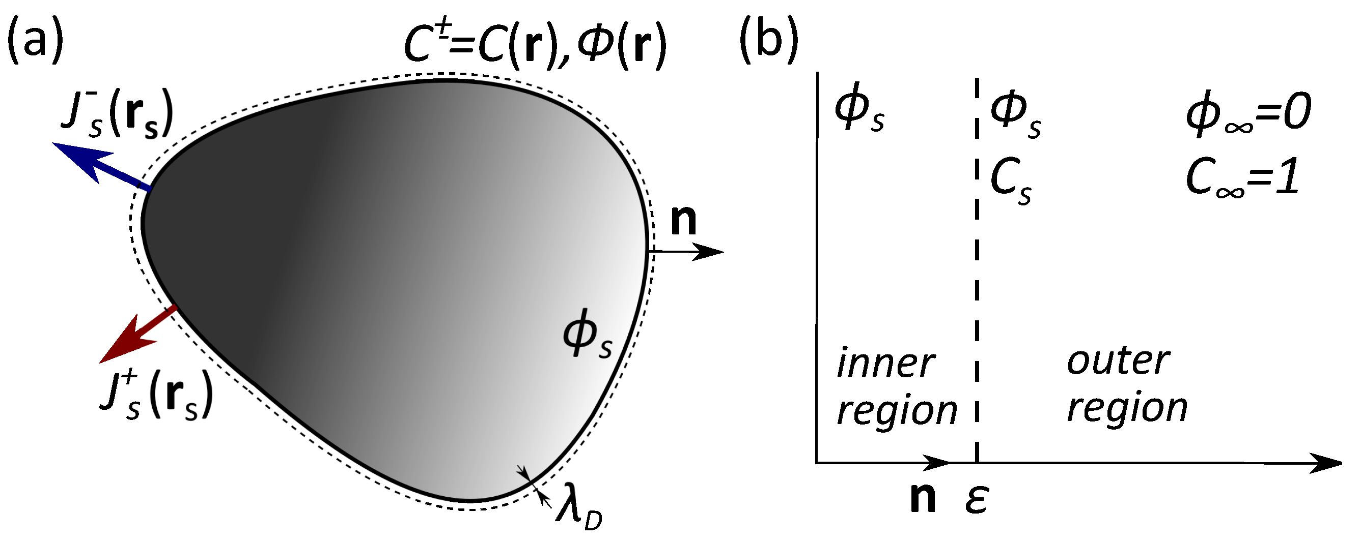
One imagines a particle of an arbitrary shape and uniform surface potential ${\varphi }_s$ in contact with a reservoir of 1:1 electrolyte solution of permittivity $ϵ$ and concentration $c_{\infty }$ (see Figure 1a). Note that, here and below, the potentials are scaled by $k_{B}T/e,$ where e is the elementary positive charge, $k_B$ is the Boltzmann constant, and T is the temperature. This ion-containing solution builds up a so-called electrostatic diffuse layer (EDL) close to the particle where the surface charge is balanced by the cloud of counterions. The extension of the EDL is defined by the Debye length of a bulk electrolyte solution, ${\lambda }_D={\left(8\pi e^2{c}_{\infty }/ϵk_{B}T\right)}^{-1/2}$. We consider that a particle can release both cations and anions, and assume that the fluxes of the released ions vary along the surface, but are not necessarily piecewise constant. These emerging at surface cations and anions diffuse towards the bulk solution. A corollary is the concentration gradients arising at distances comparable to the particle size. Since the diffusion rates of cations and anions are different, in addition, an electric field is induced. This field slows down (speeds up) ions with greater (smaller) diffusion coefficients, thus maintaining the electro-neutrality of the solution. Thus, to find the migration (phoretic) velocity of the particle, quantitative calculations of the inhomogeneous concentrations and potential are required.

The basic assumptions of our model are as follows. We might argue that for microparticles, the Reynolds number and the ratio $\lambda D/a$ are always small, as is the Peclet number for a typical ionic diffusivity. This will be used in our analytical calculations, but we do not make any further assumptions.

The ion fluxes are governed by dimensionless NP equations [3]:

$$\nabla ·{\mathbf{J}}^{\pm }=0,{\mathbf{J}}^{\pm }=\nabla C^{\pm }\pm C^{\pm }\nabla \Phi .$$

(1)

Here, the upper (lower) sign corresponds to positive (negative) ions, and $\Phi$ is a dimensionless local potential. The coordinates are scaled by a (characteristic) particle size $a,$ the concentrations $C^{\pm }$ by $c_{\infty }$. In turn, the fluxes ${\mathbf{J}}^{\pm }$ are scaled by $D^{+}{c}_{\infty }/a,$ where $D^{+}$ is the diffusion coefficient of cations. The first term in (1) represents the diffusion flux, while the second one is associated with the flux due to ion electrophoresis. Note that, in Equation (1), we neglect convective fluxes by assuming that the Peclet number is low.

An arising electric field is described by the Poisson equation for the electric potential,

$${\nabla }^2\Phi =\frac{C^{+}-C^{-}}{2{\epsilon }^2},$$

(2)

where $\epsilon ={\lambda }_D/a\ll 1$.

To solve the system of Equations (1) and (2), we have to apply the boundary conditions. Far from the particle, we deal with bulk electrolyte, so that we can naturally impose

$$\begin{array}{c}r\to \infty :C^{+}=C^{-}=1,\end{array}$$

(3)

$$\begin{array}{c}\Phi ={\varphi }_{\infty }=0.\end{array}$$

(4)

We also set the ion fluxes at the particle surface S (defined by $\mathbf{r}={\mathbf{r}}_{\mathbf{s}}$),

$$\begin{array}{c}\mathbf{r}\in S:{\mathbf{J}}^{+}·\mathbf{n}=J_s^{+}\left(\mathbf{r}\right),\end{array}$$

(5)

$$\begin{array}{c}{\mathbf{J}}^{-}·\mathbf{n}=\frac{D^{+}}{D^{-}}{J}_s^{-}\left(\mathbf{r}\right),\end{array}$$

(6)

$$\begin{array}{c}\Phi ={\varphi }_s\left(\mathbf{r}\right).\end{array}$$

(7)

The dimensionless fluxes and potential in (5)–(7) are assumed to be $O\left(1\right).$

Since the system of Equations (1) and (2) is non-linear, its general solution cannot be obtained. However, it can be simplified for some experimentally relevant cases. The particle size a is usually large compared to the Debye length ${\lambda }_D,$ so we only consider the case of $\epsilon \ll 1.$ If so, an asymptotic solution of the system of PDEs can be constructed using the method of matched expansions in two regions with different lengthscales. The lengthscale of the outer region is a and that for the inner region is ${\lambda }_D.$ We denote the potential and concentration at the dividing surface between the inner and outer regions as ${\Phi }_s\ne {\varphi }_s$ and $C_s$ (see Figure 1b).

If $\epsilon \ll 1,$ the leading-order solution of (2) for the outer region is

$$C^{+}=C^{-}=C,$$

(8)

meaning that the electroneutrality holds here to $O\left({\epsilon }^2\right).$ However, one should take into account small $C^{+}-C^{-}=O\left({\epsilon }^2\right)$, since this induces a finite potential difference in the outer region. The system (1) then becomes

$$\begin{array}{ccc}\hfill {\nabla }^{2}C+\nabla ·\left(C\nabla \Phi \right)& =& 0,\hfill \end{array}$$

(9)

$$\begin{array}{ccc}\hfill {\nabla }^{2}C-\nabla ·\left(C\nabla \Phi \right)& =& 0.\hfill \end{array}$$

(10)

Summing up and subtracting Equations (9) and (10), we obtain [7,8]

$$\begin{array}{ccc}\hfill {\nabla }^{2}C& =& 0,\hfill \end{array}$$

(11)

$$\begin{array}{ccc}\hfill \nabla ·\left(C\nabla \Phi \right)& =& 0,\hfill \end{array}$$

(12)

The latter two equations were derived earlier only for a situation of $J_s^{-}=0$. The methods of a solution of the Laplace Equation (11) are, of course, well known. However, integrating Equation (12) for the potential remains challenging. It was performed earlier for a linear case only, when the surface flux is weak, $\left|J_s^{\pm }\right|\ll 1,$ and concentration disturbances are small, so that $C\simeq 1$. In this case, Equation (12) is simplified to the Laplace equation for the potential.

Likewise, by calculating the sum and difference of Equations (5) and (6), we find

$$\begin{array}{c}\mathbf{r}\in S:\nabla C·\mathbf{n}=\frac{D^{-}{J}_s^{+}+D^{+}{J}_s^{-}}{2D^{-}},\end{array}$$

(13)

$$\begin{array}{c}C\nabla \Phi ·\mathbf{n}=\frac{D^{-}{J}_s^{+}-D^{+}{J}_s^{-}}{2D^{-}}.\end{array}$$

(14)

Solving differential Equation (12) with boundary condition (14) allows one to obtain the potential ${\Phi }_s$ of the dividing surface from the outer solution. We note that condition (7) refers to the particle surface and can be applied in the inner region only.

Since the inner region is thin it microscopically appears that the outer liquid slips over the particle surface. Provided that the Reynolds number is low, the apparent slip velocity is given by [13]:

$${\mathbf{v}}_s={\nabla }_s{\Phi }_s\left({\varphi }_s-{\Phi }_s\right)+4{\nabla }_s\left(ln{C}_s\right)ln\left[cosh\left(\frac{{\varphi }_s-{\Phi }_s}{4}\right)\right],$$

(15)

where ${\nabla }_s$ is the gradient operator along the particle surface. The first term here is associated with an electro-osmotic contribution to the slip velocity, while the second term reflects a diffusio-osmotic one.

When field variations in the outer region are small, $C\simeq 1$ and $\Phi \ll 1,$ Equation (15) can be linearised to give

$${\mathbf{v}}_s={\varphi }_s{\nabla }_s{\Phi }_s+4{\nabla }_s\left(ln{C}_s\right)ln\left[cosh\left(\frac{{\varphi }_s}{4}\right)\right].$$

(16)

The particle velocity can be calculated as the surface integral of the distribution of the apparent slip velocity [14]

$${\mathbf{v}}_p=-\frac{1}{S}\int {\mathbf{v}}_{s}dS.$$

(17)

We stress that the equations formulated in this Section are general and valid for particles of any shape, as well as for any distribution and intensity of ion fluxes at the particle surface. Some of them have, of course, been reported before, but only for specific situations or geometries.

3. Results and Examples

The main mathematical challenge is to solve non-linear Equation (12) for an outer potential. Once it is found, the self-propulsion velocity of the microswimmers can be readily calculated.

To illustrate the use of the model, we here consider the case of the constant ratio of the fluxes of two ion species at the particle surface

$$J_s^{-}\left(\mathbf{r}\right)/J_s^{+}\left(\mathbf{r}\right)=\alpha ,$$

(18)

where $\alpha$ is an arbitrary constant.

In this case, the solution of (12) satisfying the boundary conditions (4) and (14) is

$$\Phi =-\beta ln\left(C\right),$$

(19)

$$\beta ={\displaystyle \frac{\alpha D^{+}-D^{-}}{\alpha D^{+}+D^{-}}}.$$

(20)

Although at first glance Equation (18) may appear as a crude model, it incorporates the two main experimentally relevant cases of $\alpha =0$ and $\alpha =1$. Below, we shall see that they correspond to swimmers of the first and second types, correspondingly.

In the former case, $J_s^{-}=0$ and $\beta =-1$. This means that only cations are released from the particle surface. Such a situation takes place for swimmers of the first type, e.g., the Pt-Au colloids in the hydrogen peroxide solution [7,8]. In the steady state, the net flux should vanish

$$\int J_s^{+}dS=0,$$

(21)

and (19) becomes equivalent to the Boltzmann distribution for anions

$$C=exp\Phi .$$

(22)

In the latter case, $\beta =\frac{D^{+}-D^{-}}{D^{+}+D^{-}}$ and the surface fluxes of anions and cations are equal, $J_s^{-}\left(\mathbf{r}\right)=J_s^{+}\left(\mathbf{r}\right).$ Such specific swimmers of the second type are known to adequately model the enzymatic motors [9,10,11,12].

The simplest solution for a phoretic self-propulsion velocity can be obtained for a spherical particle. We naturally use a spherical coordinate system $(r,\theta )$, where the radial distance is scaled by a, and formulate boundary conditions using the so-called Damköhler number $\mathrm{Da}$, which is characteristic of ion excess near the particle. When $\mathrm{Da}\ll 1$, the surface flux is weak, and the system is close to equilibrium, so that $C\simeq 1$. However, if $\mathrm{Da}\sim 1$, the concentration of the released ions is comparable to the bulk one, and we deal with a highly non-equilibrium system. Below, we illustrate calculations of the electric potential and the self-propulsion velocity for the two types of swimmers specified above.

If $\alpha =0$ (swimmers of the first type), the simplest axisymmetric boundary condition can probably be formulated as

$$r=1:{\partial }_{r}C=\mathrm{Da}cos\theta ,$$

(23)

with $\mathrm{Da}=J_0^{+}/2$, where $J_0^{+}$ is the maximal flux of the released cations. Condition (23) was simply chosen to satisfy the condition of zero net flux (21). The solution of the Laplace Equation (11) with the boundary condition (23) reads

$$C=1+\frac{\mathrm{Da}}{2r^2}cos\theta$$

(24)

The latter equation allows one to immediately find the inner limits of the outer solutions, $C_s=C\left(1,\theta \right)$ and ${\Phi }_s=\Phi \left(1,\theta \right),$ as well as their gradients along the particle surface in order to then calculate a distribution of the apparent slip velocity given by Equation (15). Finally, the self-propulsion velocity is calculated using Equation (17), and we perform this integration numerically.

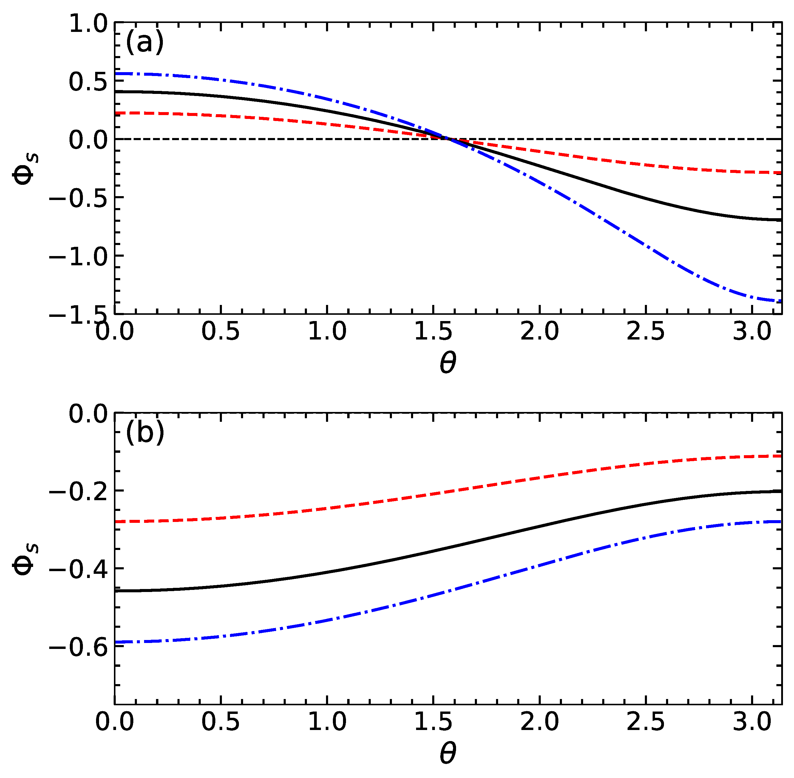
Figure 2a shows the electric potential at the dividing surface as a function of $\theta$. Calculations are made using $\alpha =0$ and several values of $\mathrm{Da}$. It can be seen that on increasing $\theta$ the function ${\Phi }_s\left(\theta \right)$ decreases and its absolute magnitude grows with $\mathrm{Da}$. ${\Phi }_s$ is positive if $\theta <\pi /2$, i.e., near the active side of the particle where the cations are released. The potential is negative when $\pi /2<\theta <\pi$, i.e., near a side that absorbs cations. The typical values of ${\Phi }_s$ are finite and, hence, should significantly influence the apparent slip velocity given by Equation (15). Indeed, since the gradients of concentration and of electric potential along the particle surface are negative, the sign of the first term in (15) is controlled by the sign of ${\varphi }_s-{\Phi }_s$. Clearly, at finite ${\Phi }_s$, the sign of this difference can in principle even reverse. Note that the second term is negative for any ${\varphi }_s-{\Phi }_s$ and that its magnitude is small compared to the first one provided this difference is small. 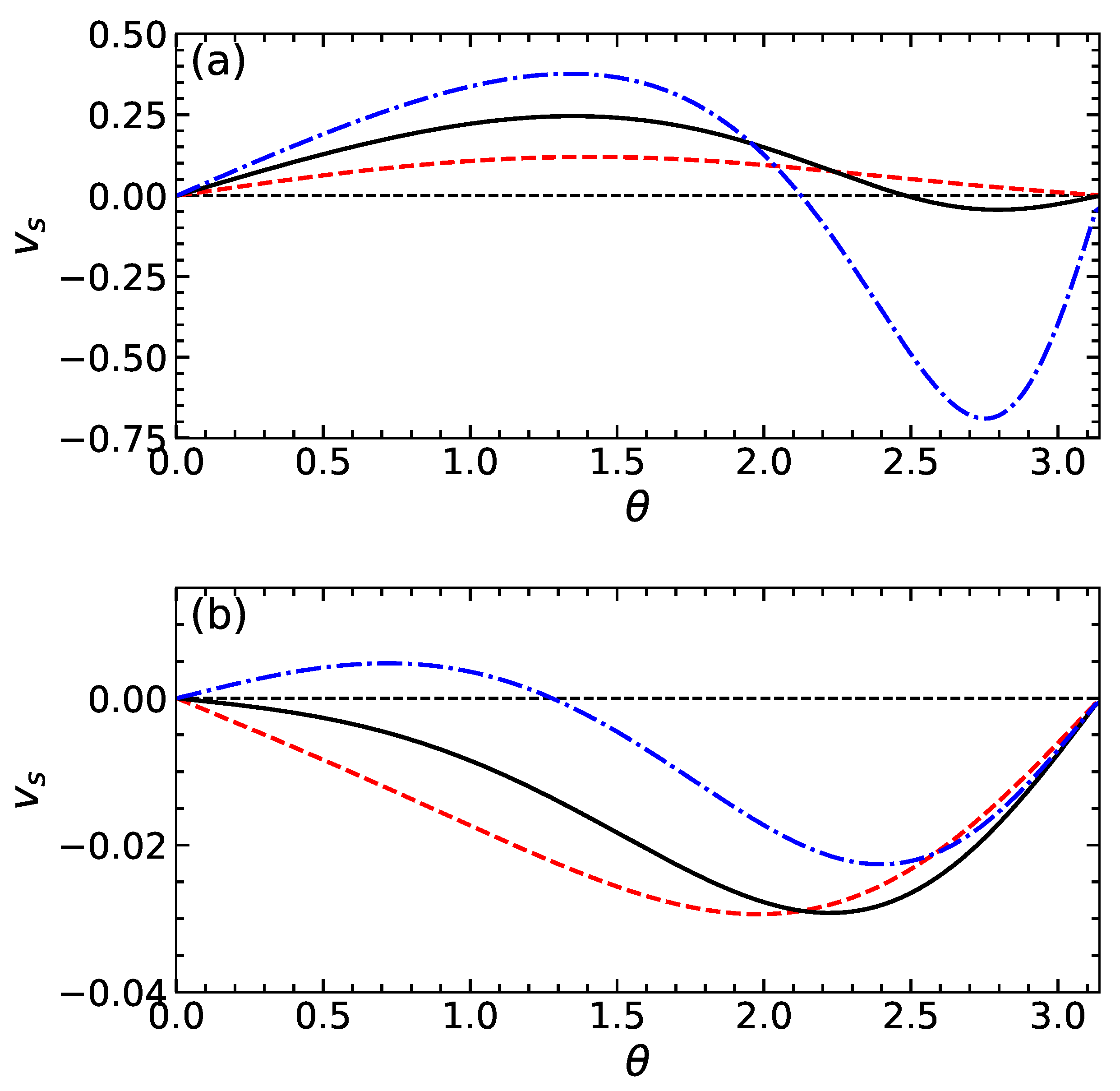Figure 3a includes the slip velocity calculated from Equation (15) using the same values of $\mathrm{Da}$ as in Figure 2a. For these calculations, we fix ${\varphi }_s=-0.5$, i.e., our particle is weakly and negatively charged. For sufficiently small $\mathrm{Da}$, the difference ${\varphi }_s-{\Phi }_s$ remains negative, so that the slip velocity is positive and takes a maximum value at $\theta \simeq \pi /2$. When $\mathrm{Da}\ge 1$, the function $v_s\left(\theta \right)$ has two extrema, and the slip velocity reverses the sign by becoming negative at some $\theta >\pi /2$. This occurs provided ${\varphi }_s-{\Phi }_s$ becomes positive as discussed above.

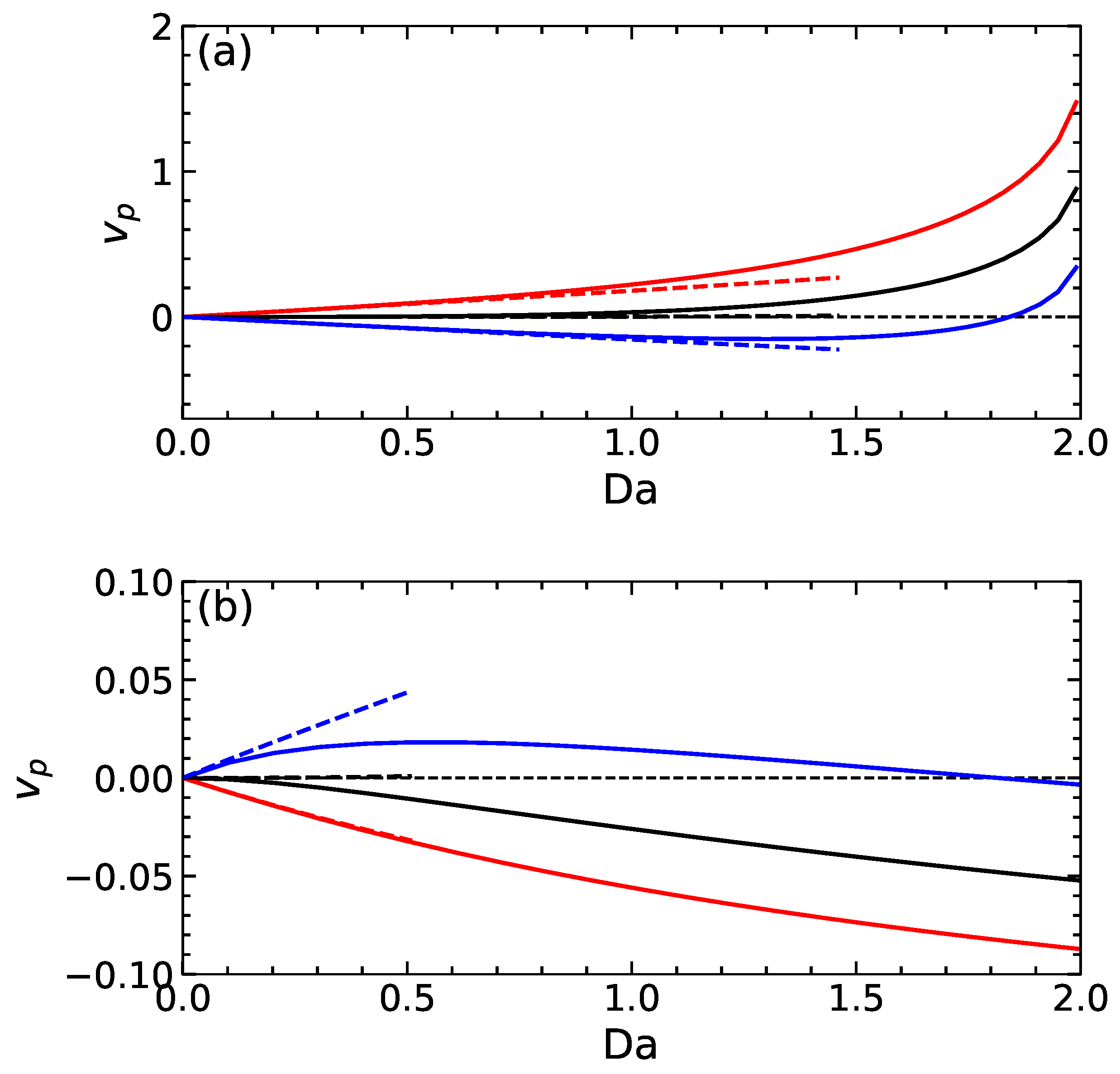
Figure 4a includes velocities $v_p$ as a function of $\mathrm{Da}$ calculated for swimmers of the first type. The calculations are made using several values of ${\varphi }_s$, which correspond to weakly charged and uncharged particles. The integral (17) is calculated on a grid $N=500$ points using the standard trapezoidal rule. It can be seen that, at $\mathrm{Da}=0$, all particles are immobile, but if we increase $\mathrm{Da}$, they start to move. The velocity of a positively charged particle is always positive. The uncharged particle remains practically immobile at relatively small $\mathrm{Da}$, but when $\mathrm{Da}=O\left(1\right)$, it propels itself in the same direction as the positively charged swimmer. Notably, the absolute value of $v_p$ highly increases non-linearly with the Damköhler number. The velocity of a negatively charged swimmer is first negative, but at some $\mathrm{Da}$, it becomes positive, i.e., the reversal of the particle velocity occurs. Furthermore, included in Figure 4a are the calculations made within a linear theory, i.e., where the apparent slip velocity was found from Equation (16). We see that the linear theory predicts that the uncharged particle remains immobile at all $\mathrm{Da}$ and that velocities of charged particles are linear in $\mathrm{Da}$. This is not surprising since both ${\nabla }_s{\Phi }_s$ and ${\nabla }_s\left(ln{C}_s\right)$ are proportional to $\mathrm{Da}$. As expected, the linear fits are quite good at small $\mathrm{Da}$, but at larger values, there is significant discrepancy.

We then consider the case of $\alpha =1$ (second type of swimmers) imposing the boundary condition

$$r=1:{\partial }_{r}C=\mathrm{Da}\left(1+cos\theta \right),$$

(25)

which ensures the positive flux over the entire surface of a sphere. The Damköhler number in this case can be expressed as $\mathrm{Da}=J_0^{+}(D^{+}+D^{-})/\left(2D^{-}\right)$, and the net ion flux is $O\left(\mathrm{Da}\right)$. The solution to (11) with the boundary condition (25) has the form

$$C=1+\frac{\mathrm{Da}}{2r}\left(2+\frac{cos\theta }{r}\right).$$

(26)

The latter equation allows us to calculate the electric potential and the apparent slip velocity, as we did in the prior example. This in turn allows one to obtain the particle velocity by the numerical integration of Equation (17).

The theoretical curves for ${\Phi }_s$ and $v_s$ are shown in Figure 2b and Figure 3b. The calculations are made with the same parameters as those used for swimmers of the first type and using $\beta =0.5$. Our results show that the potential of the dividing surface is always negative. Its gradient along the particle surface is positive and rather small. We also see that the absolute value of ${\Phi }_s$ reduces with $\theta$ and increases with $\mathrm{Da}$. As a result, the slip velocity is negative for the cases of $\mathrm{Da}=0.5$ and 1, but the situation of $\mathrm{Da}=1.5$ is different. In the latter case, it is positive at smaller $\theta$, but then, upon increasing $\theta$, it becomes negative.

Figure 4b shows the results for propulsion velocities of swimmers of the second type depending on $\mathrm{Da}$ calculated for the same values of ${\varphi }_s$ as in Figure 4a. We see that with an increasing $\mathrm{Da}$, the velocity of positively charged and neutral particles are negative and grow monotonically. An intriguing behaviour is observed for a negatively charged particle. If we increase $\mathrm{Da}$ from zero, the emerging propulsion velocity is positive, and the function $v_p\left(\mathrm{Da}\right)$ increases until it reaches a maximum. On further increasing $\mathrm{Da}$, the velocity decreases and at some $\mathrm{Da}$ becomes negative, the direction of the swimmer propulsion reverses. Interestingly, in this situation, the (negatively) charged particle propels much slower than a neutral one. Such a reversal of the direction of self-propulsion for this type of swimmer has already been found numerically [18] and also observed in the experiment [19]. Our theory gives an interpretation of the phenomenon and highlights its relevance to the potential of the dividing surface.

4. Conclusions

For catalytic swimmers of any shape, we developed a theory describing the velocity of their (phoretic) propulsion. Our mathematical model is valid for the arbitrary fluxes of ions released from their surface. The only assumptions are that the EDL should remain thin and the Peclet number small.

In our work, we employed the method of matched asymptotic expansions to find an accurate solution of the system of non-linear PDEs that describe the ion concentrations and potential near a self-propelling microparticle. Namely, from the outer solution, we determined finite potential at the dividing surface, i.e., at the outer edge of the inner region. This allowed us to find the apparent slip velocity of the liquid over the particle surface, and then calculate the velocity of the swimmer itself relative to a (stagnant) bulk electrolyte solution. As an initial example illustrating our approach, we chose a situation of the constant ratio of the fluxes of both ion species at the spherical swimmer surface, and specified two types of specific axisymmetric boundary conditions that are experimentally relevant. However, our model can be employed for more complex problems and geometries. For example, a fruitful direction could be a search for an optimal particle shape that provides the required propulsion velocity [20,21,22].

Our calculations enable one to predict and interpret several intriguing non-linear effects such as the propulsion of uncharged swimmers and the reversal of the direction of the self-propulsion of charged particles. These results are directly relevant for the self-propulsion of Pt-Au colloids induced by the catalytic decomposition of hydrogen peroxide and for chemotaxis of enzymatic motors that is currently an area of very active research.