
Minimizing Dependency Ratio in Spain through Demographic Variables


Abstract
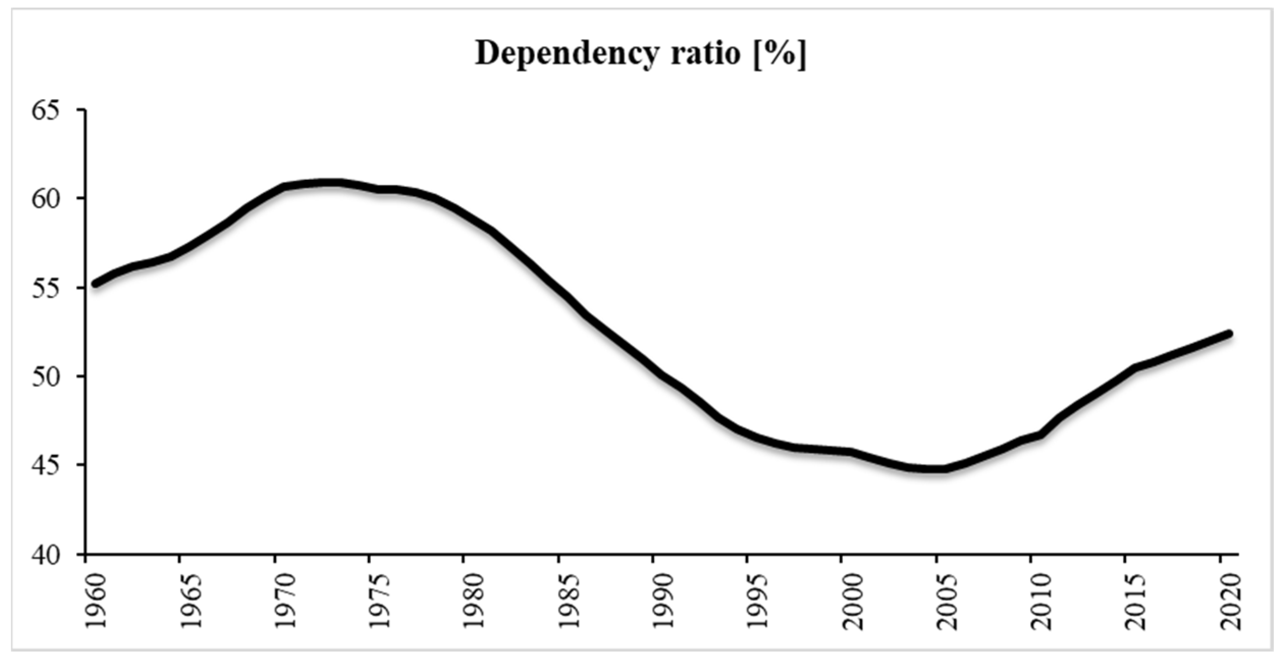
:1. Introduction
2. Materials and Methods
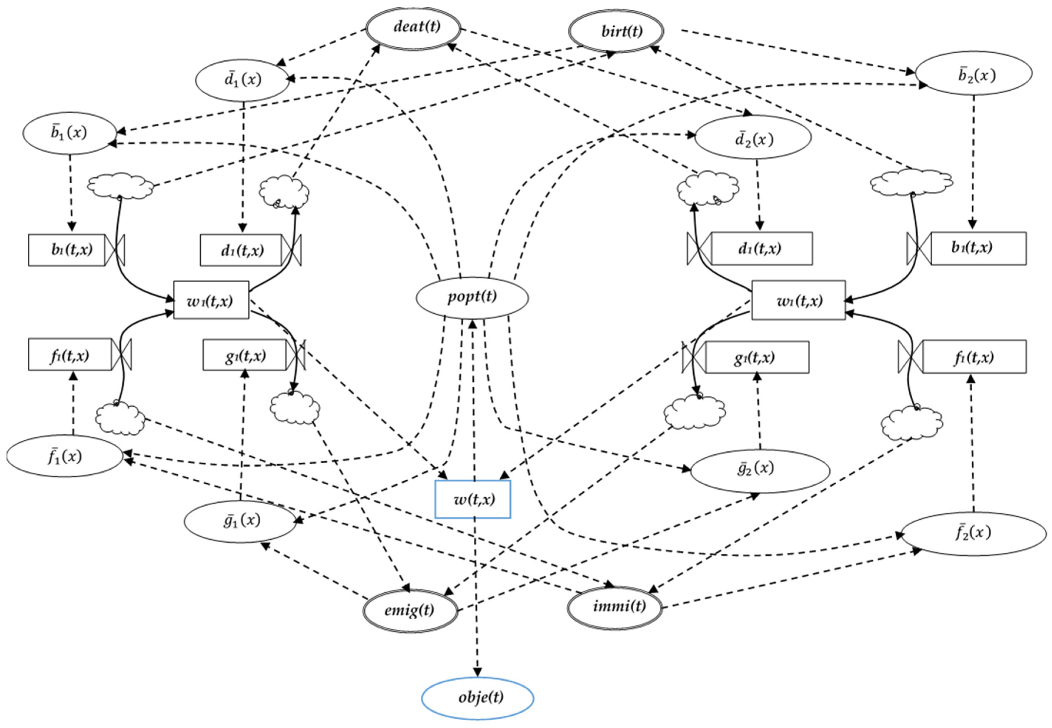
2.1. Demographic Model
2.2. Research Data
2.3. Instruments
2.3.1. Verification and Validation of the Model
2.3.2. Optimizing with Strategies and Scenarios
2.3.3. Optimizing with a Genetic Algorithm
3. Results
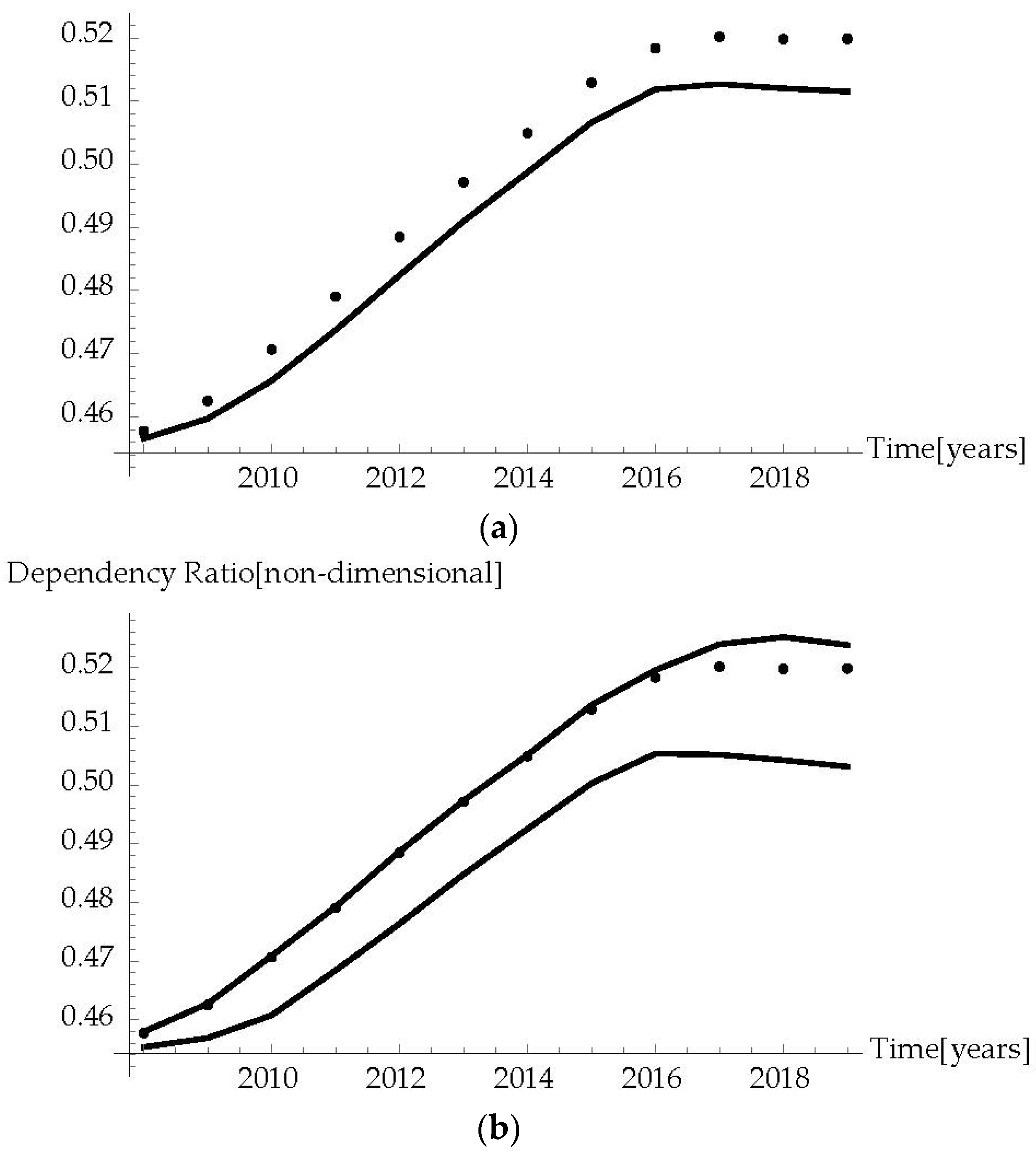
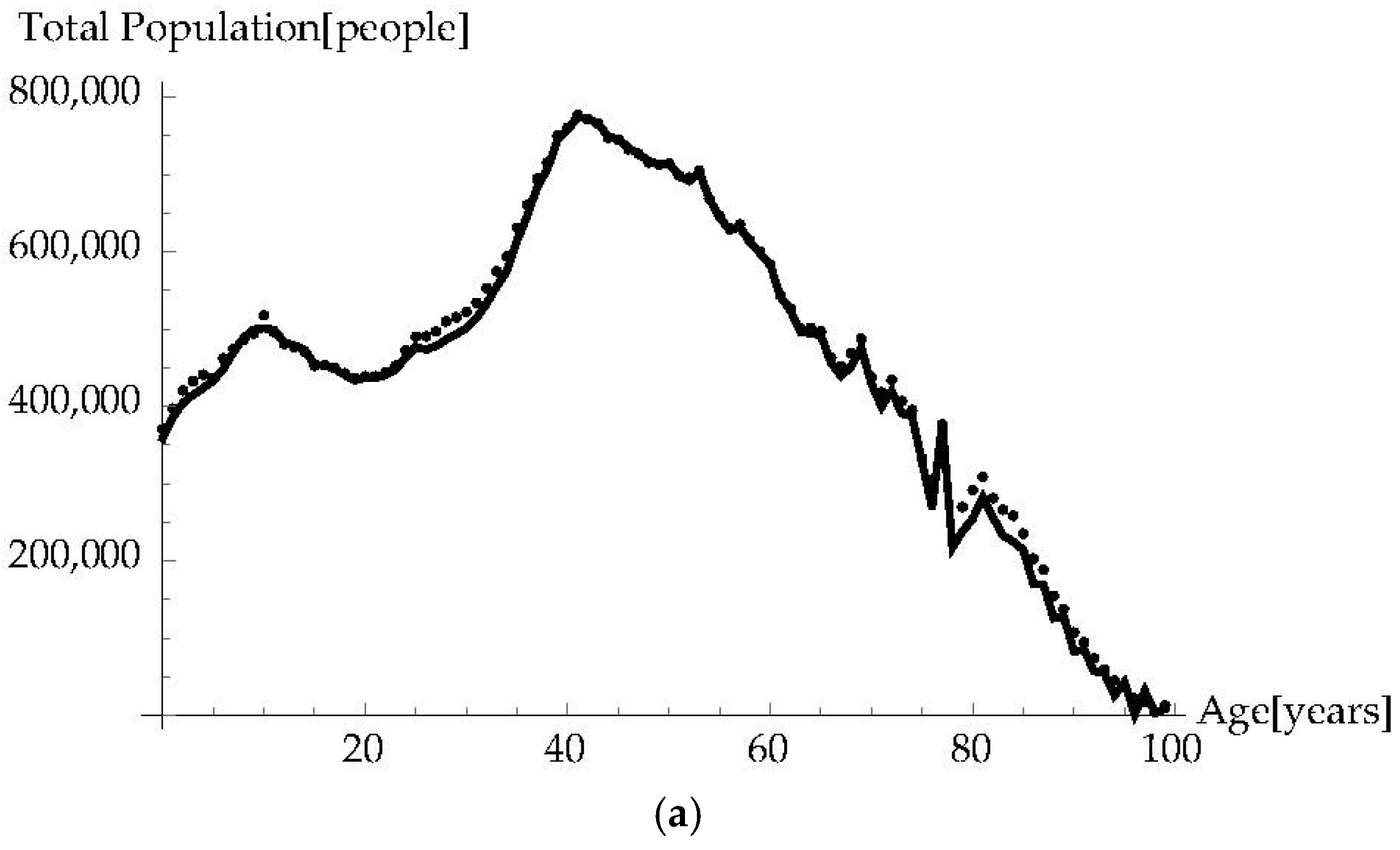
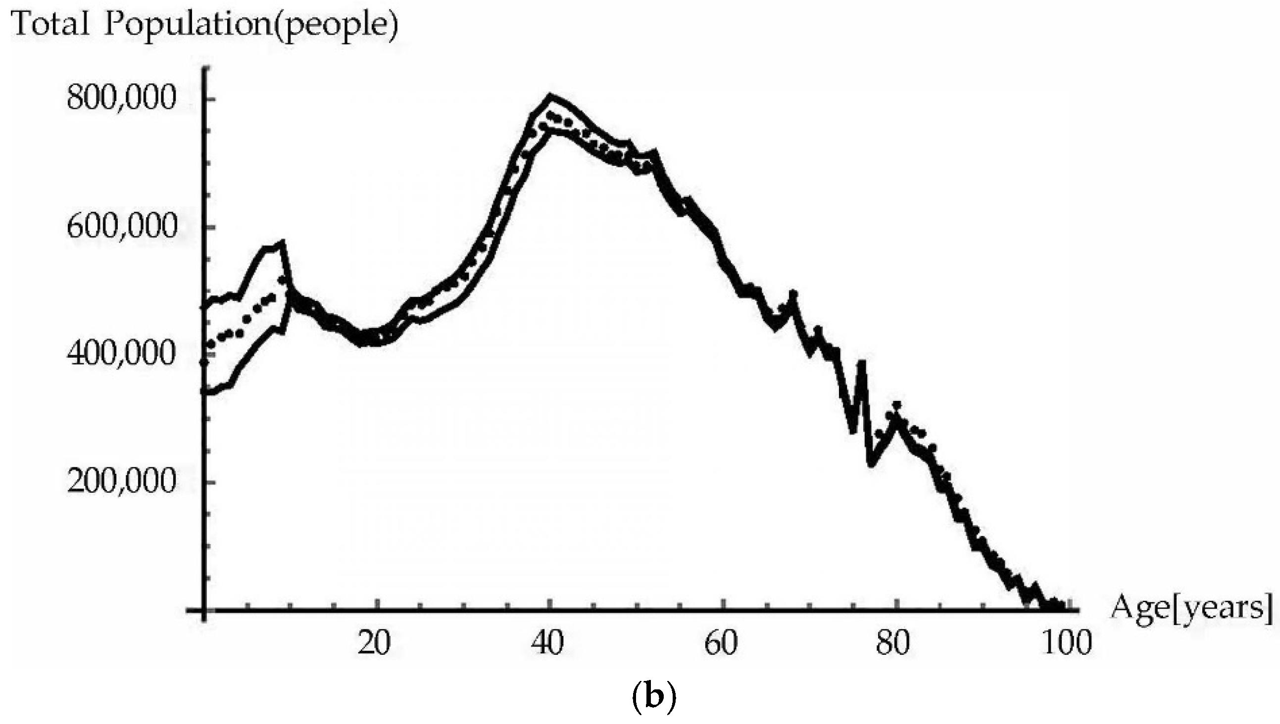
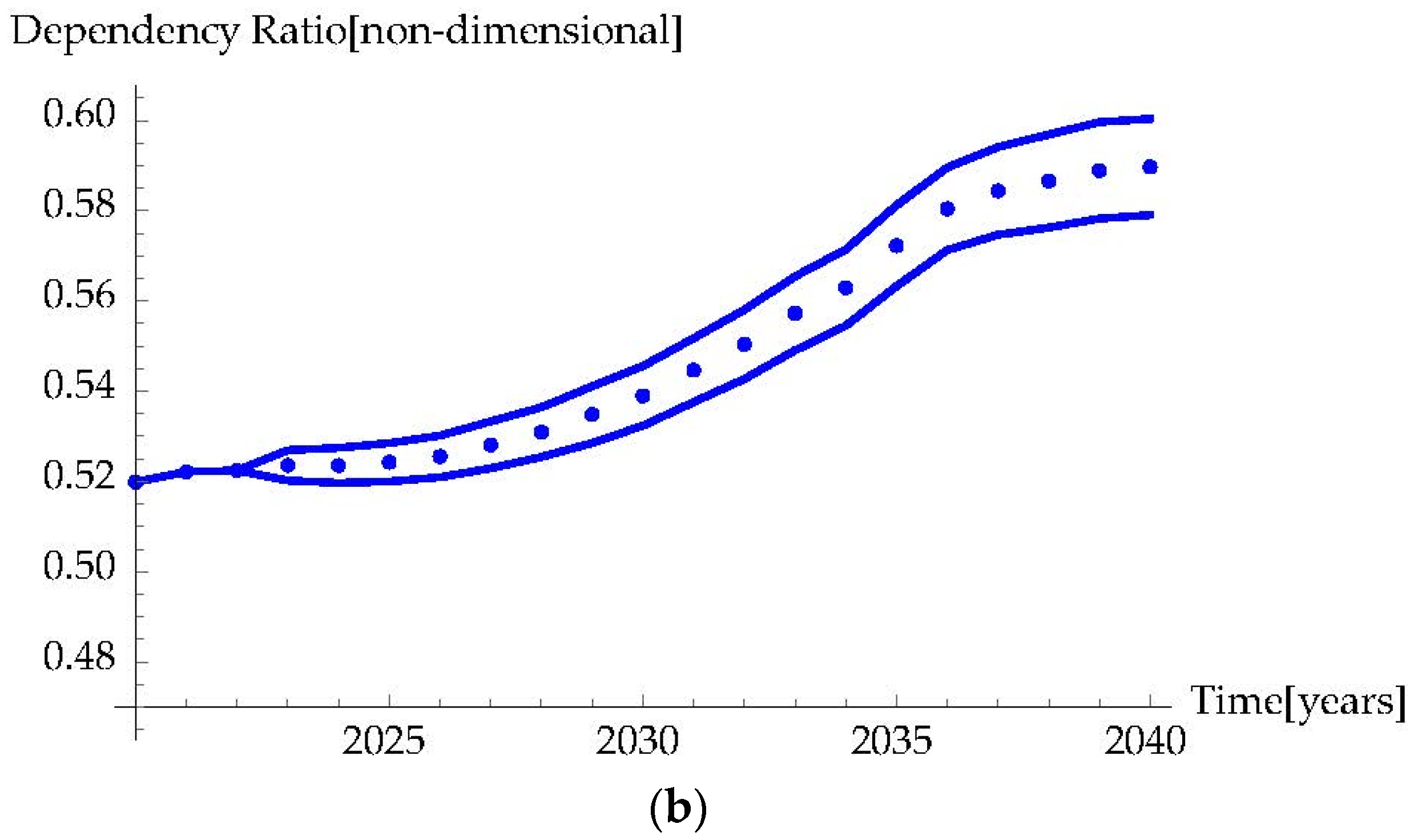
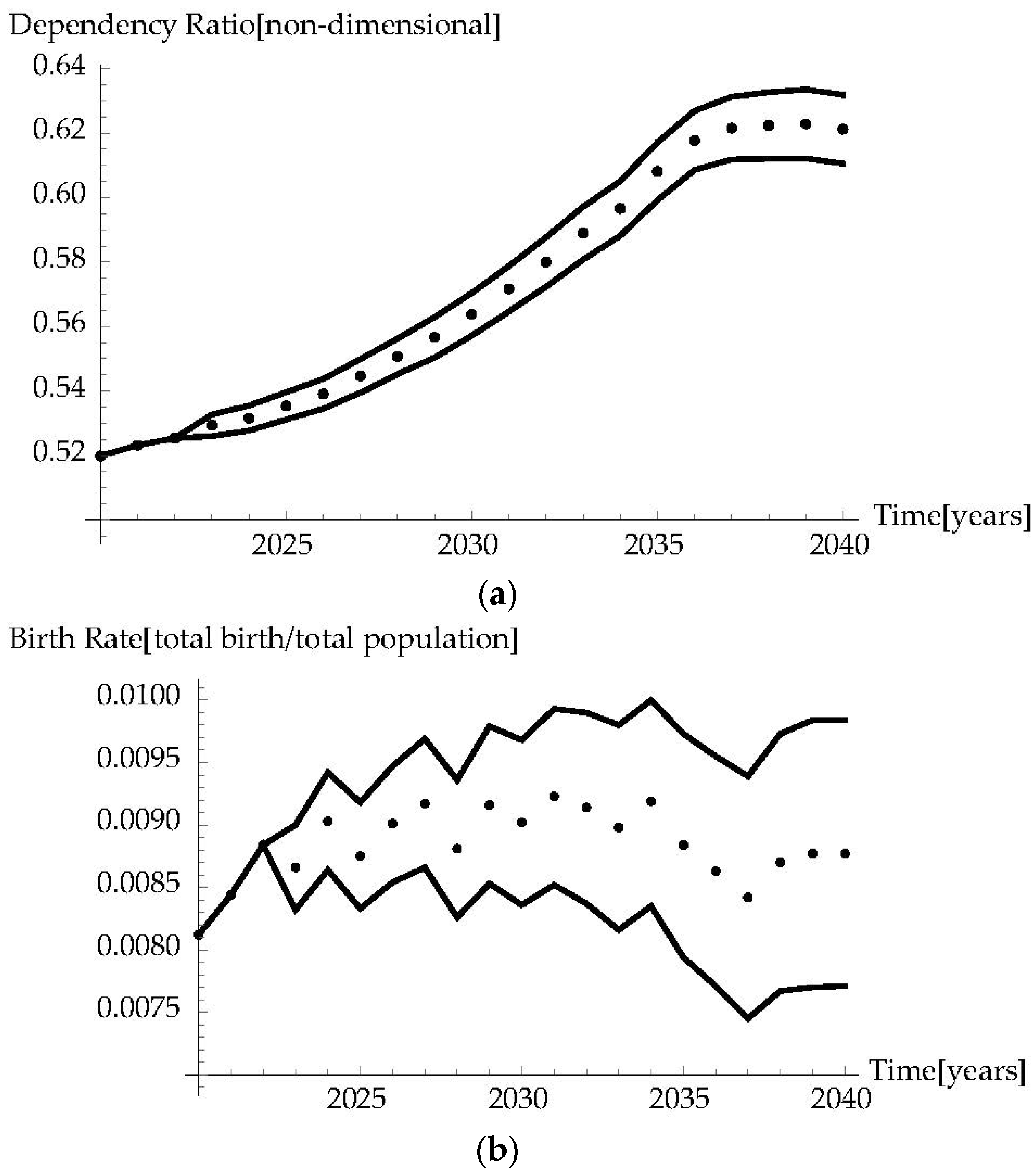
3.1. Model Verification
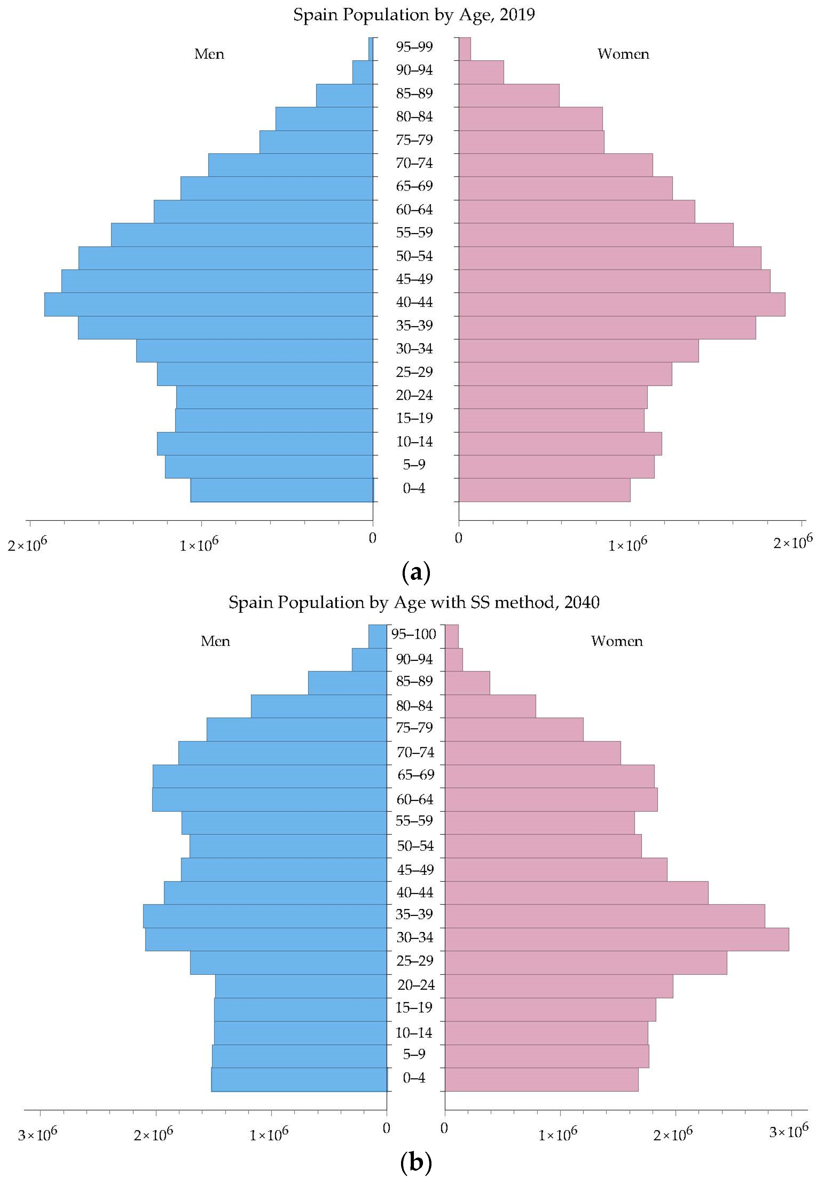
3.2. Application Case
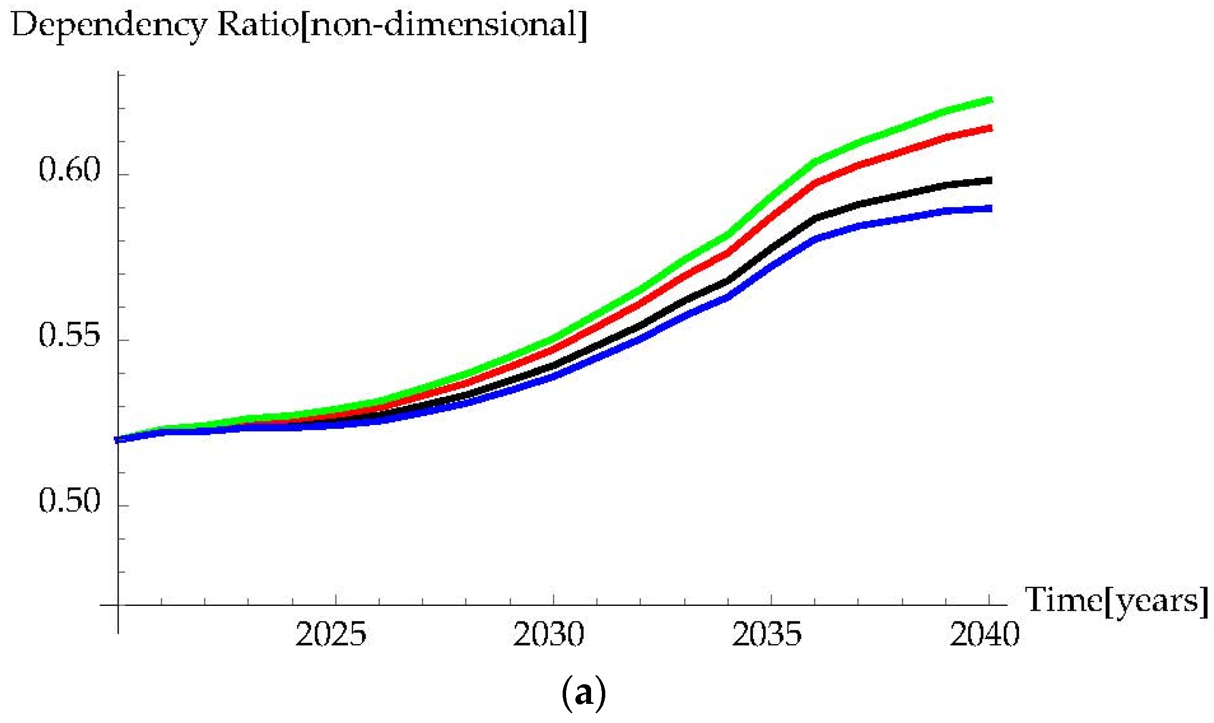
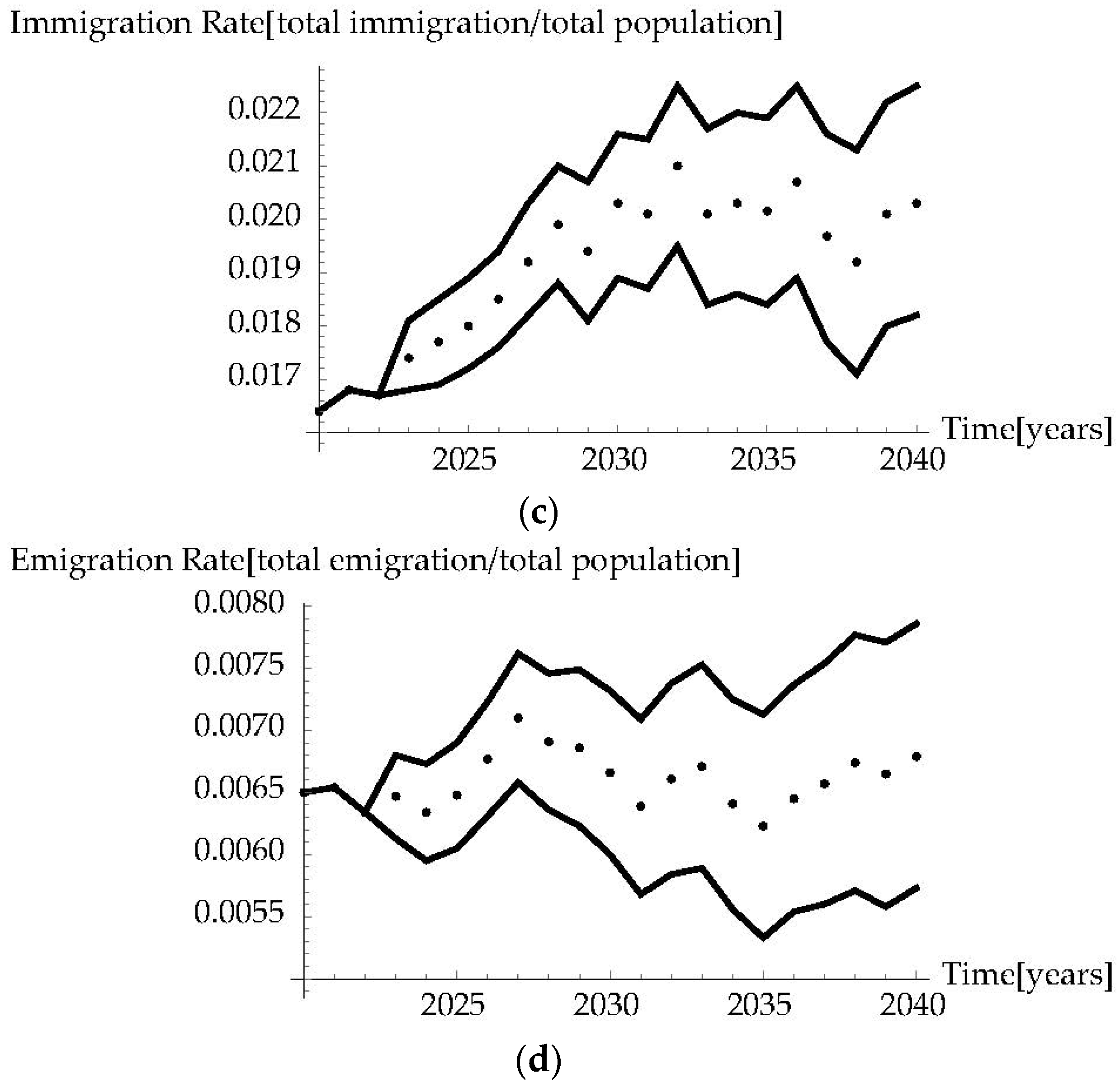
3.2.1. Strategies and Scenarios
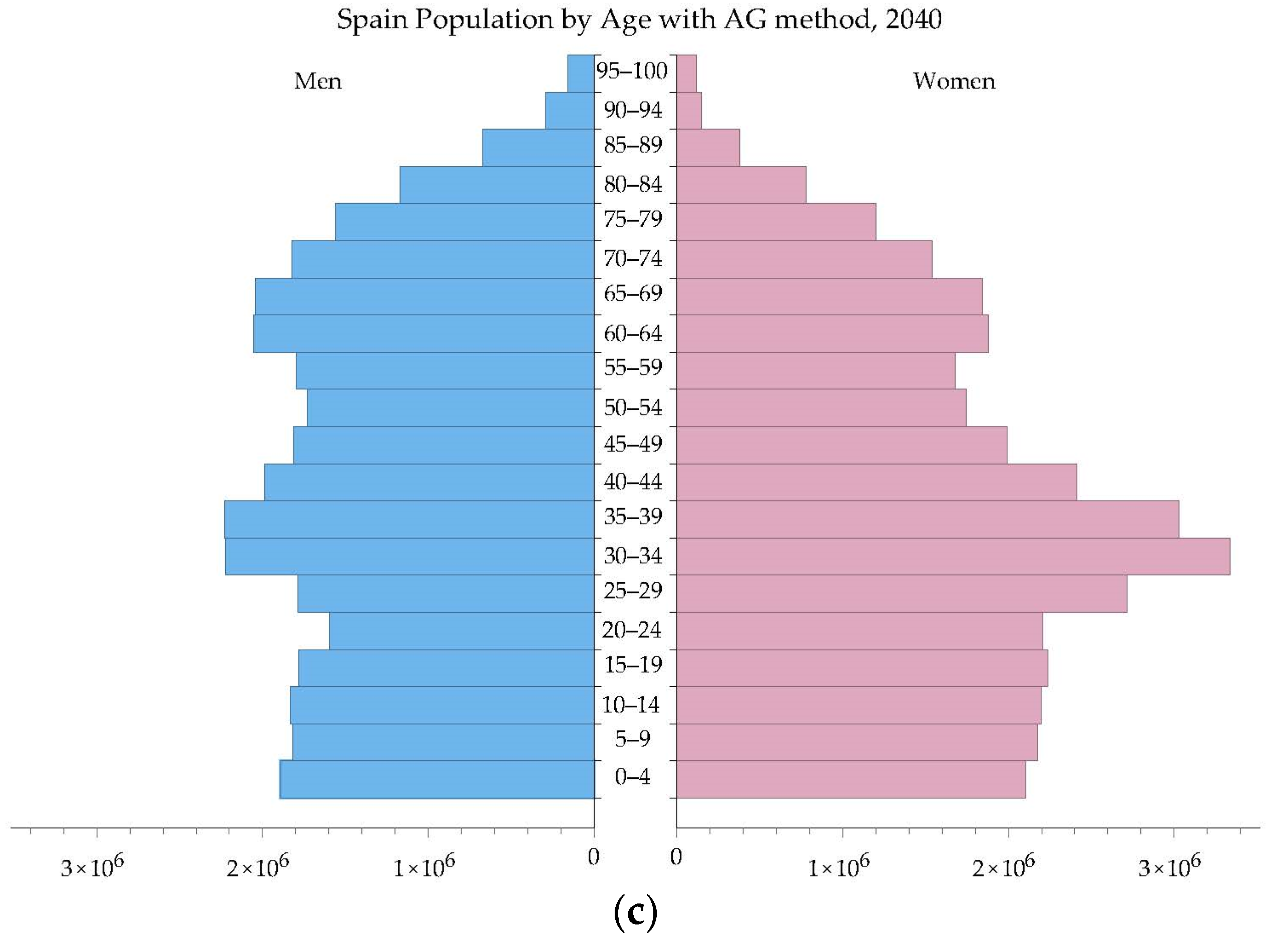
3.2.2. Genetic Algorithm
4. Discussion and Final Remarks
Author Contributions
Funding
Conflicts of Interest
Appendix A

| Acronym Variable | Database (Source) | Period |
|---|---|---|
| bi | EUROSTAT/Population and social conditions/Demography and migration/Fertility/Live births per mother’s age and newborn’s sex (demo_fasec) | 2007–2019 |
| di | EUROSTAT/Population and social conditions/Demography and migration/Mortality/Deaths per age and sex (demo_magec) | 2007–2019 |
| ei | EUROSTAT/Population and social conditions/Demography and migration//Emigration/Emigration per age and sex (migr_emi2) | 2007–2019 |
| yi | EUROSTAT/Population and social conditions/Demography and migration//Immigration/Immigration per age and sex (migr_imm8) | 2007–2019 |
| wi | EUROSTAT/Population and social conditions/Demography and migration/Population/Population on 1 January by age and sex (demo_pjan) | 2007 and 2019 |
| Year | Real Data | Minimum | Maximum |
|---|---|---|---|
| 2008 | 0.4577 | 0.4554 | 0.4580 |
| 2009 | 0.4625 | 0.4569 | 0.4628 |
| 2010 | 0.4707 | 0.4608 | 0.4709 |
| 2011 | 0.4791 | 0.4684 | 0.4793 |
| 2012 | 0.4885 | 0.4764 | 0.4887 |
| 2013 | 0.4971 | 0.4848 | 0.4974 |
| 2014 | 0.5049 | 0.4925 | 0.5051 |
| 2015 | 0.5129 | 0.5003 | 0.5136 |
| 2016 | 0.5184 | 0.5054 | 0.5196 |
| 2017 | 0.5202 | 0.5052 | 0.5240 |
| 2018 | 0.5198 | 0.5042 | 0.5252 |
| 2019 | 0.5199 | 0.5032 | 0.5239 |
| Year | Min (SS1) | Max (SS1) | Min (SS2) | Max (SS2) | Min (SS3) | Max (SS3) | Min (SS4) | Max (SS4) |
|---|---|---|---|---|---|---|---|---|
| 2020 | 0.520 | 0.520 | 0.520 | 0.520 | 0.520 | 0.520 | 0.520 | 0.520 |
| 2021 | 0.522 | 0.522 | 0.523 | 0.523 | 0.523 | 0.523 | 0.522 | 0.522 |
| 2022 | 0.523 | 0.523 | 0.521 | 0.526 | 0.521 | 0.527 | 0.522 | 0.522 |
| 2023 | 0.521 | 0.528 | 0.522 | 0.529 | 0.523 | 0.530 | 0.520 | 0.527 |
| 2024 | 0.521 | 0.529 | 0.522 | 0.530 | 0.524 | 0.531 | 0.520 | 0.527 |
| 2025 | 0.521 | 0.530 | 0.523 | 0.532 | 0.525 | 0.533 | 0.520 | 0.529 |
| 2026 | 0.522 | 0.532 | 0.524 | 0.535 | 0.527 | 0.536 | 0.521 | 0.530 |
| 2027 | 0.525 | 0.536 | 0.528 | 0.539 | 0.530 | 0.541 | 0.523 | 0.533 |
| 2028 | 0.528 | 0.539 | 0.531 | 0.543 | 0.534 | 0.546 | 0.525 | 0.536 |
| 2029 | 0.532 | 0.544 | 0.535 | 0.549 | 0.538 | 0.552 | 0.529 | 0.541 |
| 2030 | 0.536 | 0.549 | 0.540 | 0.555 | 0.543 | 0.557 | 0.532 | 0.546 |
| 2031 | 0.541 | 0.555 | 0.546 | 0.562 | 0.550 | 0.565 | 0.538 | 0.552 |
| 2032 | 0.547 | 0.562 | 0.552 | 0.570 | 0.557 | 0.574 | 0.543 | 0.558 |
| 2033 | 0.554 | 0.570 | 0.560 | 0.578 | 0.566 | 0.583 | 0.549 | 0.565 |
| 2034 | 0.559 | 0.576 | 0.567 | 0.586 | 0.572 | 0.591 | 0.555 | 0.571 |
| 2035 | 0.569 | 0.587 | 0.577 | 0.597 | 0.583 | 0.603 | 0.563 | 0.581 |
| 2036 | 0.577 | 0.596 | 0.587 | 0.608 | 0.593 | 0.615 | 0.571 | 0.590 |
| 2037 | 0.581 | 0.601 | 0.592 | 0.613 | 0.598 | 0.621 | 0.575 | 0.594 |
| 2038 | 0.583 | 0.604 | 0.596 | 0.617 | 0.603 | 0.625 | 0.576 | 0.597 |
| 2039 | 0.585 | 0.608 | 0.601 | 0.621 | 0.607 | 0.631 | 0.578 | 0.600 |
| 2040 | 0.586 | 0.610 | 0.604 | 0.624 | 0.610 | 0.635 | 0.579 | 0.600 |
References
- Age Dependency Ratio. Available online: https://data.worldbank.org/indicator/SP.POP.DPND (accessed on 28 February 2022).
- Available online: https://esa.un.org/poppolicy/publications.aspx (accessed on 28 February 2022).
- Simon, C.; Belyakov, A.O.; Feichtinger, G. Minimizing the dependency ratio in a population with below-replacement fertility through immigration. Theor. Popul. Biol. 2012, 82, 158–169. [Google Scholar] [CrossRef] [PubMed] [Green Version]
- Cruz, M.; Ahmed, S.A. On the impact of demographic change on economic growth and poverty. World Develp. 2018, 105, 95–106. [Google Scholar] [CrossRef]
- Samir, K.C.; Lutz, W. The human core of the shared socioeconomic pathways: Population scenarios by age, sex and level of education for all countries to 2100. Glob. Environ. Chang. 2017, 42, 181–192. [Google Scholar] [CrossRef] [Green Version]
- Estructura Demográfica y Envejecimiento de la Población. Available online: http://ec.europa.eu/eurostat/statistics-explained/index.php/Population_structure_and_ageing/es (accessed on 28 February 2022).
- United, N. Replacement Migration: Is It a Solution to Declining and Ageing Populations? United Nations Publications: New York, NY, USA, 2001. [Google Scholar]
- Schmertmann, C.P. Stationary populations with below-replacement fertility. Demogr. Res. 2012, 26, 319–330. [Google Scholar] [CrossRef] [Green Version]
- Micó, J.C.; Soler, D.; Sanz, M.T.; Caselles, A.; Amigó, S. Birth rate and population pyramid: A stochastic dynamical model. In Modelling for Engineering & Human Behaviour 2018, Valencia, Spain, 16–18 July 2018; Jodar, L., Cortes, J.C., Alcedo, L., Eds.; Universitat Politécnica de Valencia: Valencia, Spain, 2018; pp. 292–297. [Google Scholar]
- Micó, J.C.; Soler, D.; Sanz, M.T.; Caselles, A.; Amigó, S. Optimizing the demographic rates to control the dependency ratio in Spain. In Modelling for Engineering & Human Behaviour 2019, Valencia, Spain, 10–12 July 2019; Company, R., Cortes, J.C., Jodar, L., Lopez-Navarro, E., Eds.; Universitat Politécnica de Valencia: Valencia, Spain, 2019; pp. 193–198. [Google Scholar]
- Eurostat. Available online: https://ec.europa.eu/eurostat/data/database (accessed on 28 February 2022).
- Forrester, J.W. The City. Urban Dynamics; MIT Press: Cambridge, UK, 1969. [Google Scholar]
- Djidjeli, K.; Price, W.G.; Temarel, P.; Twizell, E.H. Partially implicit schemes for the numerical solutions of some non-linear differential equations. Appl. Math. Comput. 1998, 96, 177–207. [Google Scholar] [CrossRef]
- Letellier, C.; Elaydi, S.; Aguirre, L.A.; Alaoui, A. Difference equations versus differential equations, a possible equivalence for the Rossler system? Phys. D Nonlin. Phen. 2004, 195, 29–49. [Google Scholar] [CrossRef] [Green Version]
- Canh, N.T. El Desafío de la Población (The Population Challenge). Sesión Pública del Sudeste Asiático, Vietnam. 2003. Available online: http://www.eurosur.org/futuro/03.htm (accessed on 28 February 2022).
- Marchetti, C.; Meyer, P.S.; Ausubel, J.H. Human population dynamics revisited with the logistic model: How much can be modeled and predicted? Technol. Forecast. Soc. Chang. 1996, 52, 1–30. [Google Scholar] [CrossRef] [Green Version]
- Caselles, A. A tool for discovery by complex function fitting. In Cybernetics and Systems Research’98; Trappl, R., Ed.; Austrian Society for Cybernetic Studies: Vienna, Austria, 1998; pp. 787–792. [Google Scholar]
- Caselles, A. Modelización y Simulación de Sistemas Complejos (Modeling and Simulation of Complex Systems); Universitat de València: Valencia, Spain, 2008; Available online: https://www.uv.es/caselles/Mod1.pdf (accessed on 28 February 2022).
- Sanz, M.T. Modelo Socio-Demográfico Dinámico Para el Estudio de la Sostenibilidad Demográfica Desde Factores Calidad de Vida. Ph.D. Thesis, Universidad Politécnica de Valencia, Valencia, Spain, 2012. [Google Scholar]
- Caselles, A.; Soler, D.; Sanz, M.T.; Micó, J.C. A Methodology for Modeling and Optimizing Social Systems. Cybern. Syst. 2020, 51, 265–314. [Google Scholar] [CrossRef]
- Secretaría General Para el Reto Demográfico. Proyecciones Población del Instituto Nacional de Estadística y Previsiones Demográficas de la Autoridad Independiente de Responsabilidad Fiscal. Available online: https://www.google.com/search?client=firefox-b-d&q=PROYECCIONES+POBLACI%C3%93N+DEL+INSTITUTO+NACIONAL+DE+ESTAD%C3%8DSTICA+Y+PREVISIONES+DEMOGR%C3%81FICAS+DE+LA+AUTORIDAD+INDEPENDIENTE+DE+RESPONSABILIDAD+FISCAL# (accessed on 28 February 2022).
- Marois, G.; Bélanger, A.; Lutz, W. Population aging, migration, and productivity in Europe. Proc. Natl. Acad. Sci. USA 2020, 117, 7690–7695. [Google Scholar] [CrossRef] [PubMed] [Green Version]
- Conde-Ruiz, J.I.; González, C.I. Estudios Sobre la Economía Española—2021/07; El Proceso de Envejecimiento en España; Fedea: Madrid, Spain, 2021; Available online: https://www.google.com/search?client=firefox-b-d&q=eee2021-07# (accessed on 28 February 2022).


| Control Variable | SS1 | SS2 | SS3 | SS4 |
|---|---|---|---|---|
| Birth rate | ↑ | ↑ | ↑ | ↑ |
| Emigration rate | ↑ | ↓ | ↑ | ↓ |
| Immigration rate | ↑ | ↓ | ↓ | ↑ |
| CROM | CROI | Minimum PCRO | Maximum PCRO |
|---|---|---|---|
| CROM(1) Birth rate | 0.00784 | 0.00784 | 0.0200 |
| CROM(2) Immigration rate | 0.01632 | 0.00500 | 0.0350 |
| CROM(3) Emigration rate | 0.00644 | 0.00482 | 0.0200 |
Publisher’s Note: MDPI stays neutral with regard to jurisdictional claims in published maps and institutional affiliations. |
© 2022 by the authors. Licensee MDPI, Basel, Switzerland. This article is an open access article distributed under the terms and conditions of the Creative Commons Attribution (CC BY) license (https://creativecommons.org/licenses/by/4.0/).
Share and Cite
Micó, J.C.; Soler, D.; Sanz, M.T.; Caselles, A.; Amigó, S. Minimizing Dependency Ratio in Spain through Demographic Variables. Mathematics 2022, 10, 1471. https://doi.org/10.3390/math10091471
Micó JC, Soler D, Sanz MT, Caselles A, Amigó S. Minimizing Dependency Ratio in Spain through Demographic Variables. Mathematics. 2022; 10(9):1471. https://doi.org/10.3390/math10091471
Chicago/Turabian StyleMicó, Joan C., David Soler, Maria T. Sanz, Antonio Caselles, and Salvador Amigó. 2022. "Minimizing Dependency Ratio in Spain through Demographic Variables" Mathematics 10, no. 9: 1471. https://doi.org/10.3390/math10091471