
Deep Learning XAI for Bus Passenger Forecasting: A Use Case in Spain


Abstract
:1. Introduction
2. Related Works
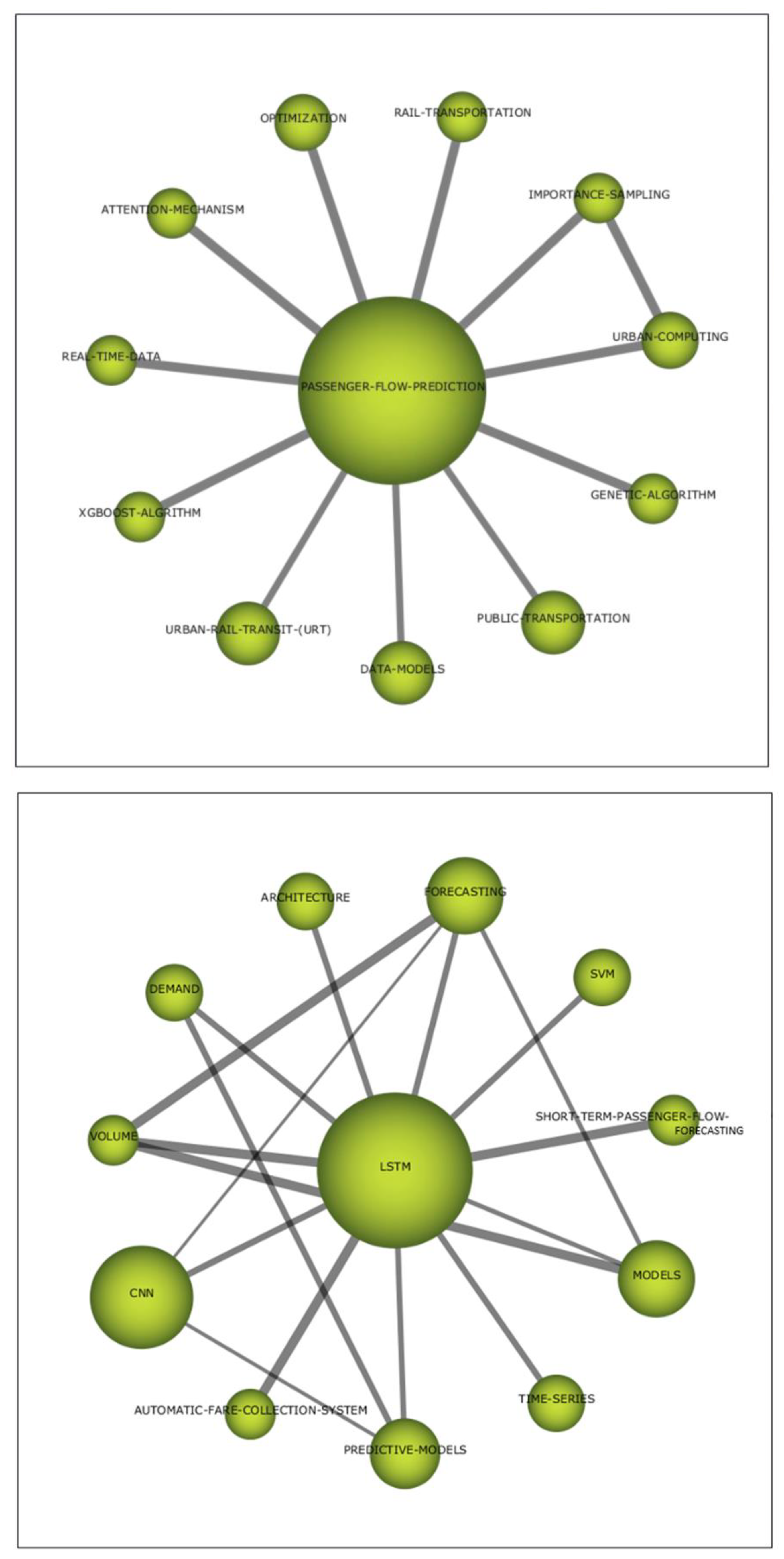
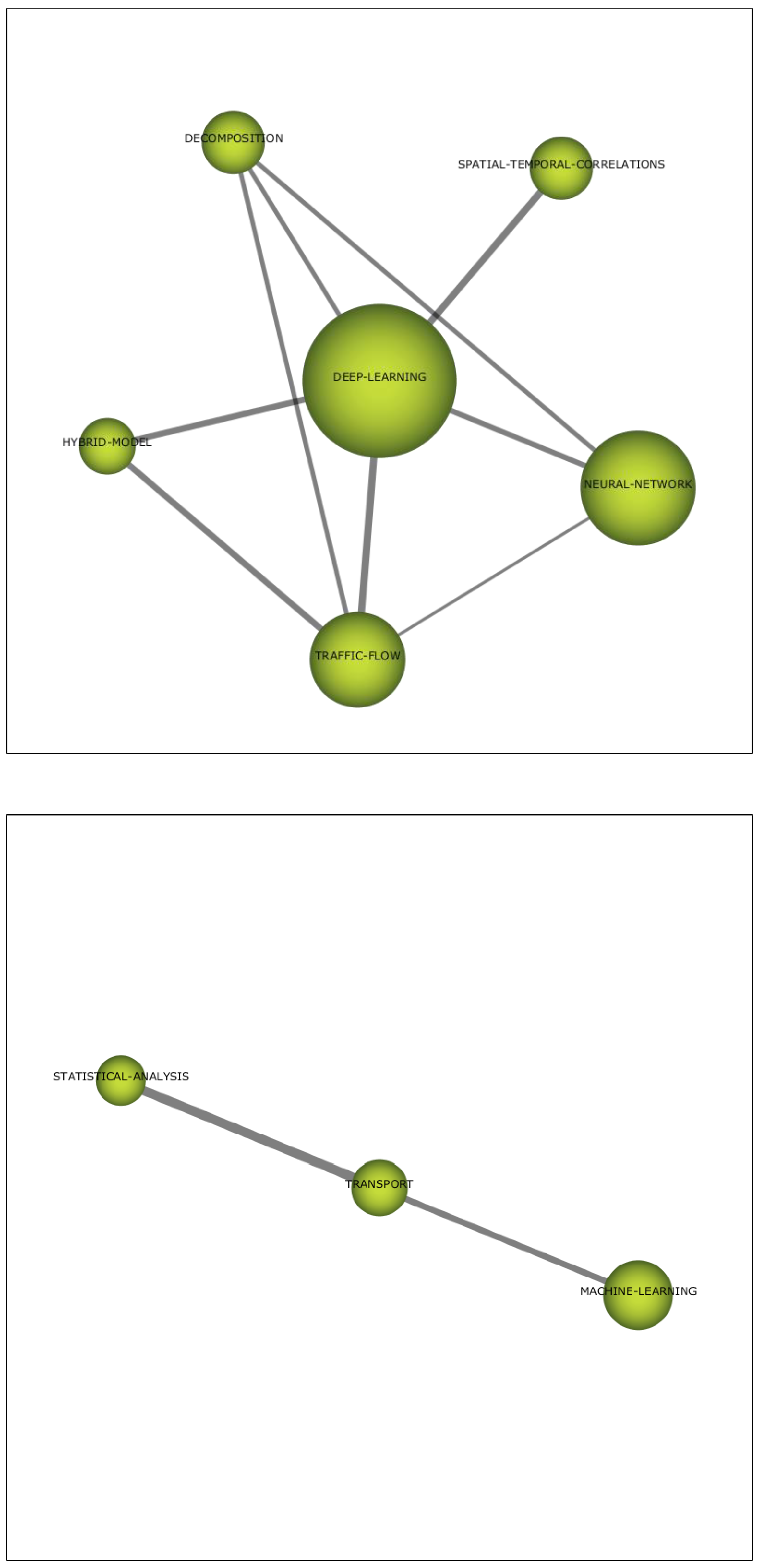
- DEEP-LEARNING. Based on neural networks, this algorithms are widely used for the traffic flow prediction problem presented here.
- LSTM. This theme includes specific deep/machine learning algorithms which are important or motor for the problem at hand. Thus, LSTM models are the central and predominant topic, the Convolutional Neural Networks (CNN) are in second place, and finally, Support Vector Machine (SVM) is much less prominent. The theme is related with time model prediction since in the problems we are dealing with, they are very common.
- PASSENGER-FLOW-PREDICTION. This is a heterogeneous topic that includes the optimization problems and techniques studied, including genetic algorithms. It also includes other predictive techniques such as XGBoost. This theme includes other interesting terms that point to the use of real-time data and predictive applications on urban and public transportation.
- TRANSPORT. This is a very small and declining theme which includes the use of statistical analysis and generic machine learning for the problem posed.
3. Methodology
3.1. The 2-Tuple Fuzzy Linguistic Model
- If , then is less than .
- If , then
- (a)
- If , then and represent the same information.
- (b)
- If , then is less than .
- (c)
- If , then is greater than .
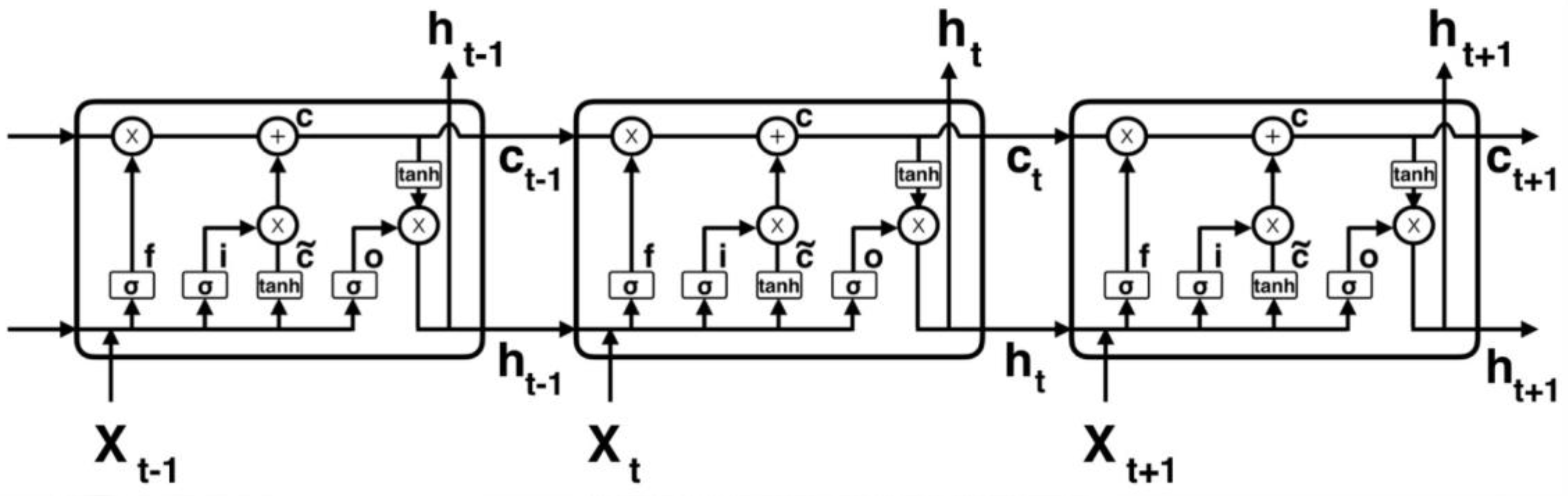
3.2. LSTM Model
3.3. Surrogate Trees and Rules
- Select the dataset X used to train the black box model.
- For the selected dataset X, get the predictions of the black box model.
- Select a regression tree model.
- Train the regression tree on the dataset X and its predictions.
- Obtaining the rules from the regression tree.
- Measure how well the surrogate model replicates the predictions of the black box model.
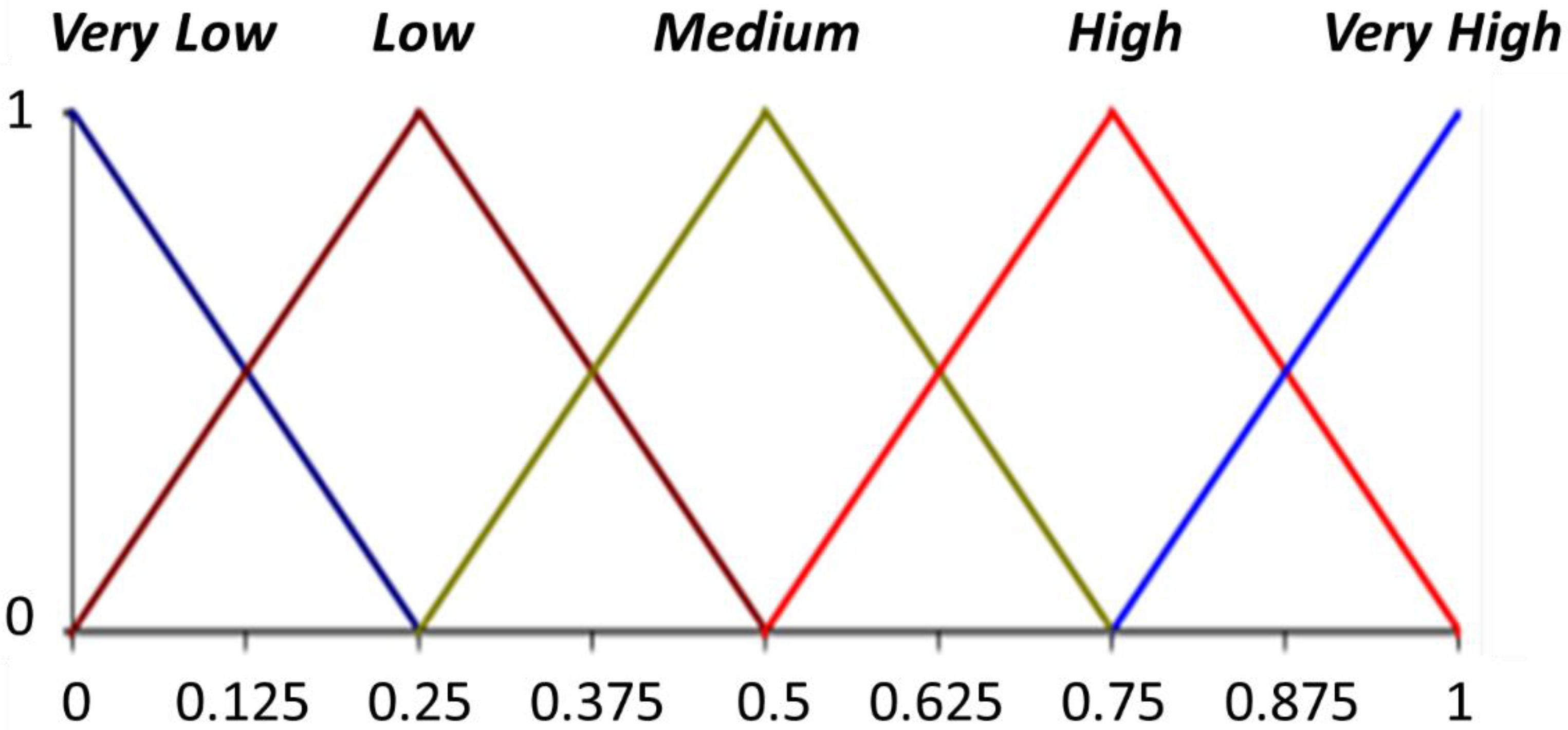
- Fuzzification of the variable to be predicted using the fuzzy 2-tuple linguistic model.
- Interpret the surrogate fuzzy linguistic model.
4. Proposed Model
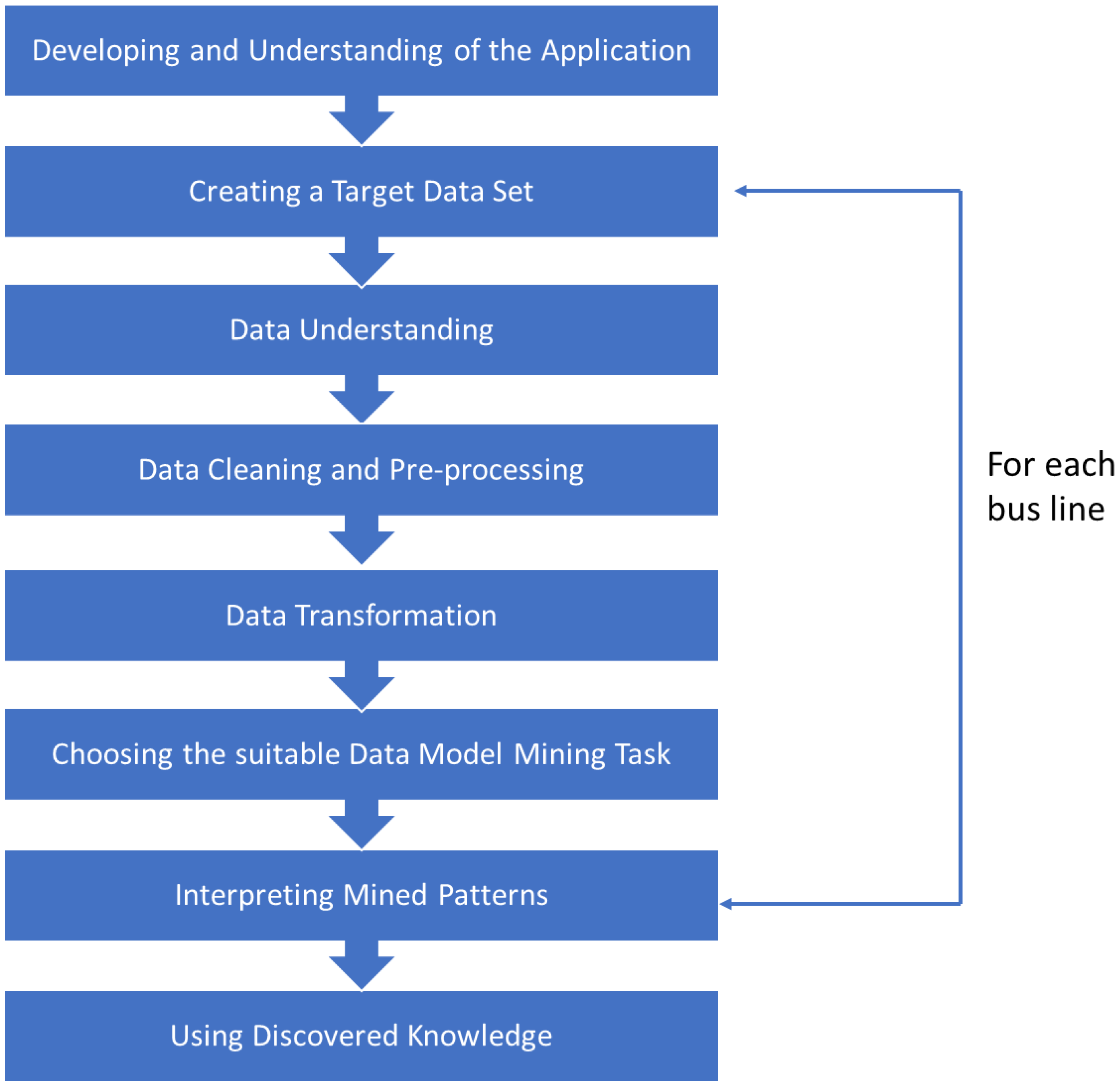
4.1. Developing and Understanding of the Application
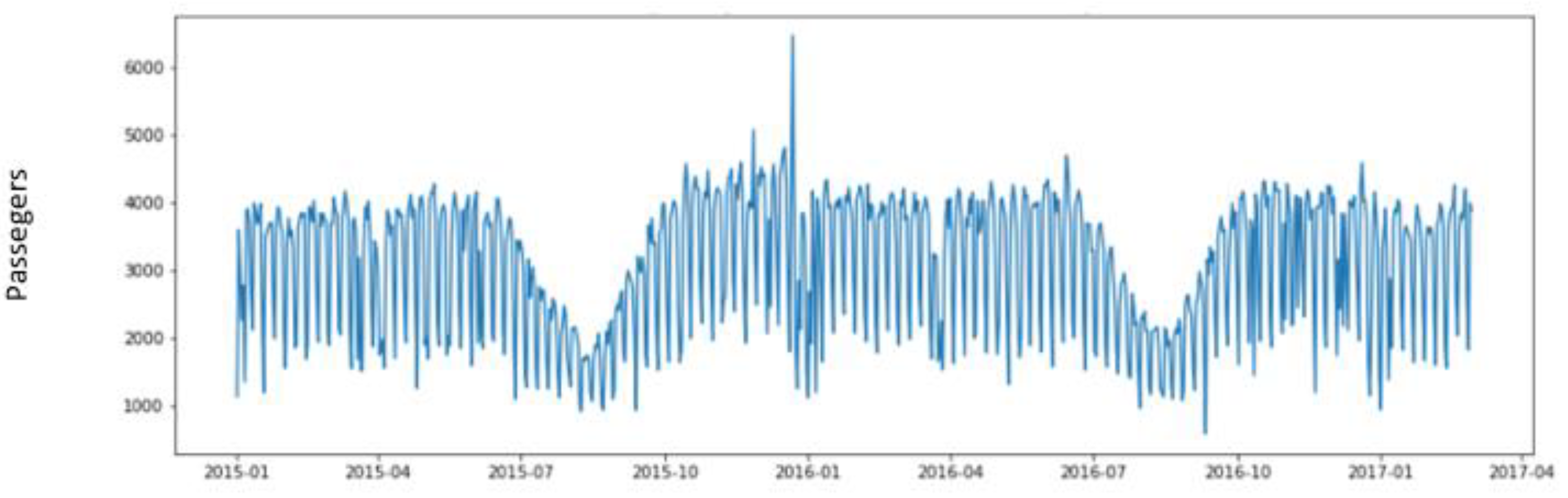
4.2. Creating a Target Data Set
- -
- Date: Field that indicates the date formed by year, month and day (e.g., 20160101);
- -
- Passengers: number of passengers in the selected time slot.
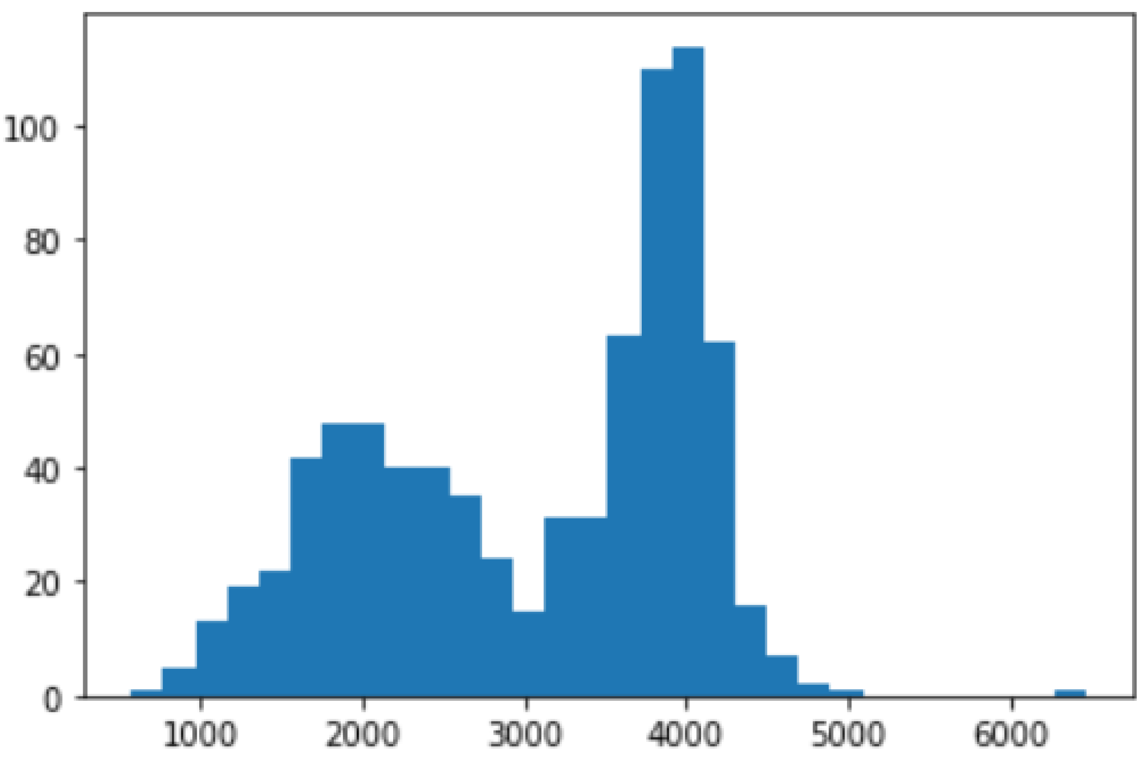
4.3. Data Understanding
- -
- Date: Field that indicates the date formed by year, month and day;
- -
- Month: indicates the month (e.g., January = 1);
- -
- Holiday; 1: yes, 0: no;
- -
- Day of week: indicates the day of week (e.g., Monday = 0);
- -
- Passengers: number of passengers.
4.4. Data Cleansing and Pre-Processing
4.5. Data Transformation
- -
- day of week: Mon., Tue., Wed., Thu., Fri., Sat., Sun.;
- -
- month: Jan., Feb., March, April, May, June, July, Aug., Sept., Oct., Nov., Dec.
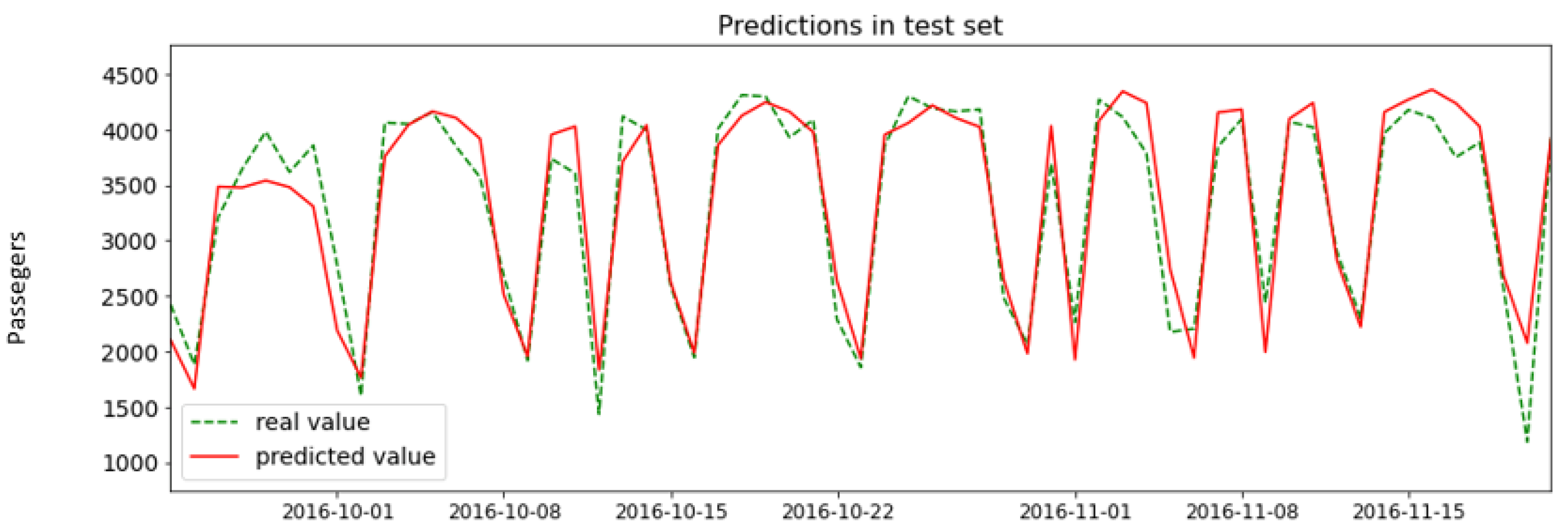
4.6. Choosing the Most Suitable ML Algorithm
4.7. Interpreting Mined Patterns
4.8. Using Discovered Knowledge
5. Discussion
- Rule 1: very high demand. Days that are not summer days and are neither weekends nor holidays. That is, days when people go about their daily routine.
- Rule 2: high demand. Days in September that are neither weekends nor holidays. In Madrid, the demand for passengers increases in the month of September because most of the population is already working and the schools are starting the academic year.
- Rule 3: Days in July that are neither weekends nor holidays. On those days, students do not have to attend classes and from the second fortnight onwards, some workers start their vacations. Therefore, passenger demand starts to decrease.
- Rule 4: Saturdays when passenger demand on the eve was very high. A large part of the population does not work on Saturday afternoons. On those days, public transport is usually used for leisure activities, so passenger demand is lower than on the eve.
- Rule 5: Holiday that are not weekends or days in August. It seems that during those holidays people prefer to stay at home or move to other areas.
- Rule 6. August days that are not weekends. In August many companies close and workers have to take mandatory vacations. In addition, students do not have to go to class, so passenger demand declines.
- Rule 7. Saturdays where passenger demand on the eve was high/medium. Same interpretation as in Rule 4.
- Rule 8. Sundays where passenger demand on the eve was not low or very low. The activities carried out by people in Madrid are similar on Saturdays and Sundays, but many street stores are closed on Sundays. For this reason, passenger demand on these two days is similar, with a lower demand on Sundays.
- Rule 9. Sundays where passenger demand on the eve was very low. Same interpretation as in Rule 8.
6. Conclusions and Future Work
Author Contributions
Funding
Institutional Review Board Statement
Informed Consent Statement
Data Availability Statement
Acknowledgments
Conflicts of Interest
References
- Spirin, I.; Zavyalov, D.; Zavyalova, N. Globalization and development of sustainable public transport systems. In Proceedings of the 16th International Scientific Conference Globalization and Its Socio-Economic Consequences, Rajecke Teplice, Slovakia, 5–6 October 2016; Volume 5, pp. 2076–2084. [Google Scholar]
- Li, W.; Sui, L.; Zhou, M.; Dong, H. Short-term passenger flow forecast for urban rail transit based on multi-source data. EURASIP J. Wirel. Commun. Netw. 2021, 2021, 9. [Google Scholar] [CrossRef]
- Schmidhuber, J. Deep Learning in Neural Networks: An Overview. Neural Netw. 2015, 61, 85–117. [Google Scholar] [CrossRef] [PubMed] [Green Version]
- LeCun, Y.; Bengio, Y.; Hinton, G. Deep learning. Nature 2015, 521, 436–444. [Google Scholar] [CrossRef] [PubMed]
- Hochreiter, S.; Schmidhuber, J. Long Short-Term Memory. Neural Comput. 1997, 9, 1735–1780. [Google Scholar] [CrossRef] [PubMed]
- Gers, F.A.; Schmidhuber, J.; Cummins, F. Learning to Forget: Continual Prediction with LSTM. Neural Comput. 2000, 12, 2451–2471. [Google Scholar] [CrossRef] [PubMed]
- Jiao, F.; Huang, L.; Song, R.; Huang, H. An Improved STL-LSTM Model for Daily Bus Passenger Flow Prediction during the COVID-19 Pandemic. Sensors 2021, 21, 5950. [Google Scholar] [CrossRef] [PubMed]
- Zadeh, L.A. The concept of a linguistic variable and its applications to approximate reasoning. Pt I. Inf. Sci. 1975, 8, 199–249. [Google Scholar] [CrossRef]
- Liu, H.; Ning, H.; Mu, Q.; Zheng, Y.; Zeng, J.; Yang, L.T.; Huang, R.; Ma, J. A review of the smart world. Future Gener. Comput. Syst. 2019, 96, 678–691. [Google Scholar] [CrossRef]
- Manibardo, E.L.; Laña, I.; Del Ser, J. Deep learning for road traffic forecasting: Does it make a difference? IEEE Trans. Intell. Transp. Syst. 2021, 1–25. Available online: https://ieeexplore.ieee.org/document/9447807 (accessed on 28 February 2022). [CrossRef]
- Cristóbal, T.; Padrón, G.; Quesada-Arencibia, A.; Alayón, F.; de Blasio, G.; García, C.R. Bus travel time prediction model based on profile similarity. Sensors 2019, 19, 2869. [Google Scholar] [CrossRef] [PubMed] [Green Version]
- Cobo, M.J.; López-Herrera, A.G.; Herrera-Viedma, E.; Herrera, F. SciMAT: A new science mapping analysis software tool. J. Am. Soc. Inf. Sci. Technol. 2012, 63, 1609–1630. [Google Scholar] [CrossRef]
- Lv, W.; Lv, Y.; Ouyang, Q.; Ren, Y. A Bus Passenger Flow Prediction Model Fused with Point-of-Interest Data Based on Extreme Gradient Boosting. Appl. Sci. 2022, 12, 940. [Google Scholar] [CrossRef]
- Jin, W.; Li, P.; Wu, W.; Wei, L. Short-Term Public Transportation Passenger Flow Forecasting Method Based on Multi-source Data and Shepard Interpolating Prediction Method. In International Conference on Man-Machine-Environment System Engineering; Springer: Singapore, 2018; pp. 281–294. [Google Scholar] [CrossRef]
- Ouyang, Q.; Lv, Y.; Ma, J.; Li, J. An LSTM-Based Method Considering History and Real-Time Data for Passenger Flow Prediction. Appl. Sci. 2020, 10, 3788. [Google Scholar] [CrossRef]
- Gummadi, R.; Edara, S.R. Prediction of passenger flow of transit buses over a period of time using artificial neural network. In Proceedings of the Third, International Congress on Information and Communication Technology, London, UK, 27–28 February 2018; Springer: Singapore, 2019; pp. 963–971. [Google Scholar] [CrossRef]
- Nagaraj, N.; Gururaj, H.L.; Swathi, B.H.; Hu, Y.-C. Passenger flow prediction in bus transportation system using deep learning. Multimed Tools Appl. 2022, 81, 12519–12542. [Google Scholar] [CrossRef] [PubMed]
- Zhai, H.; Tian, R.; Cui, L.; Xu, X.; Zhang, W. A novel hierarchical hybrid model for short-term bus passenger flow forecasting. J. Adv. Transp. 2020, 2020, 7917353. [Google Scholar] [CrossRef]
- Zou, L.; Shu, S.; Lin, X.; Lin, K.; Zhu, J.; Li, L. Passenger Flow Prediction Using Smart Card Data from Connected Bus System Based on Interpretable XGBoost. Wirel. Commun. Mob. Comput. 2022, 2022, 5872225. [Google Scholar] [CrossRef]
- Liu, L.; Chen, R.C. A novel passenger flow prediction model using deep learning methods. Transp. Res. Part C Emerg. Technol. 2017, 84, 74–91. [Google Scholar] [CrossRef]
- Chen, T.; Fang, J.; Xu, M.; Tong, Y.; Chen, W. Prediction of Public Bus Passenger Flow Using Spatial–Temporal Hybrid Model of Deep Learning. J. Transp. Eng. Part A Syst. 2022, 148, 04022007. [Google Scholar] [CrossRef]
- Wu, W.; Xia, Y.; Jin, W. Predicting bus passenger flow and prioritizing influential factors using multi-source data: Scaled stacking gradient boosting decision trees. IEEE Trans. Intell. Transp. Syst. 2020, 22, 2510–2523. Available online: https://ieeexplore.ieee.org/document/9284598 (accessed on 28 February 2022). [CrossRef]
- Liu, Y.; Lyu, C.; Liu, X.; Liu, Z. Automatic feature engineering for bus passenger flow prediction based on modular convolutional neural network. IEEE Trans. Intell. Transp. Syst. 2020, 22, 2349–2358. Available online: https://ieeexplore.ieee.org/document/9141203 (accessed on 28 February 2022). [CrossRef]
- Liu, W.; Tan, Q.; Wu, W. Forecast and early warning of regional bus passenger flow based on machine learning. Math. Probl. Eng. 2020, 2020, 6625435. [Google Scholar] [CrossRef]
- Tan, Q.; Ling, X.; Chen, M.; Lu, H.; Wang, P.; Liu, W. Statistical analysis and prediction of regional bus passenger flows. Int. J. Mod. Phys. B 2019, 33, 1950094. [Google Scholar] [CrossRef]
- Bai, Y.; Sun, Z.; Zeng, B.; Deng, J.; Li, C. A multi-pattern deep fusion model for short-term bus passenger flow forecasting. Appl. Soft Comput. 2017, 58, 669–680. [Google Scholar] [CrossRef]
- Han, Y.; Wang, C.; Ren, Y.; Wang, S.; Zheng, H.; Chen, G. Short-term prediction of bus passenger flow based on a hybrid optimized LSTM network. ISPRS Int. J. Geo-Inf. 2019, 8, 366. [Google Scholar] [CrossRef] [Green Version]
- Zhang, N.; Chen, H.; Chen, X.; Chen, J. Forecasting public transit use by crowdsensing and semantic trajectory mining: Case studies. ISPRS Int. J. Geo-Inf. 2016, 5, 180. [Google Scholar] [CrossRef] [Green Version]
- Luo, D.; Zhao, D.; Ke, Q.; You, X.; Liu, L.; Zhang, D.; Ma, H.; Zuo, X. Fine-grained service-level passenger flow prediction for bus transit systems based on multitask deep learning. IEEE Trans. Intell. Transp. Syst. 2020, 22, 7184–7199. Available online: https://ieeexplore.ieee.org/document/9126198 (accessed on 28 February 2022). [CrossRef]
- Wang, Y.; Currim, F.; Ram, S. Deep Learning of Spatiotemporal Patterns for Urban Mobility Prediction Using Big Data. Inf. Syst. Res. 2022. [Google Scholar] [CrossRef]
- Toqué, F.; Khouadjia, M.; Come, E.; Trepanier, M.; Oukhellou, L. Short & long term forecasting of multimodal transport passenger flows with machine learning methods. In Proceedings of the 2017 IEEE 20th International Conference on Intelligent Transportation Systems (ITSC), Yokohama, Japan, 16–19 October 2017; IEEE: Piscataway, NJ, USA; pp. 560–566. Available online: https://ieeexplore.ieee.org/document/8317939 (accessed on 28 February 2022).
- Zhai, H.; Cui, L.; Nie, Y.; Xu, X.; Zhang, W. A comprehensive comparative analysis of the basic theory of the short term bus passenger flow prediction. Symmetry 2018, 10, 369. [Google Scholar] [CrossRef] [Green Version]
- Minh, D.; Wang, H.X.; Li, Y.F.; Nguyen, T.N. Explainable artificial intelligence: A comprehensive review. Artif. Intell. Rev. 2021, 1–66. [Google Scholar] [CrossRef]
- Rawal, A.; Mccoy, J.; Rawat, D.B.; Sadler, B.; Amant, R. Recent Advances in Trustworthy Explainable Artificial Intelligence: Status, Challenges and Perspectives. IEEE Trans. Artif. Intell. 2021, 1, 1. Available online: https://www.computer.org/csdl/journal/ai/5555/01/09645355/1zc6Hmkb1xm (accessed on 28 February 2022). [CrossRef]
- Thakker, D.; Mishra, B.K.; Abdullatif, A.; Mazumdar, S.; Simpson, S. Explainable artificial intelligence for developing smart cities solutions. Smart Cities 2020, 3, 1353–1382. [Google Scholar] [CrossRef]
- Peijl, E.V.D.; Najjar, A.; Mualla, Y.; Bourscheid, T.J.; Spinola-Elias, Y.; Karpati, D.; Nouzri, S. Toward XAI & Human Synergies to Explain the History of Art: The Smart Photobooth Project. In Proceedings of the International Workshop on Explainable, Transparent Autonomous Agents and Multi-Agent Systems, Virtual Event, 3–7 May 2021; Springer: Cham, Switzerland, 2021; pp. 208–222. [Google Scholar]
- Corchado, J.; Chamoso, P.; Hernández, G.; Gutierrez, A.R.; Camacho, A.; González-Briones, A.; Pinto-Santos, F.; Goyenechea, E.; Garcia-Retuerta, D.; Alonso-Miguel, M.; et al. Deepint. net: A rapid deployment platform for smart territories. Sensors 2021, 21, 236. [Google Scholar] [CrossRef] [PubMed]
- Kostopoulos, G.; Panagiotakopoulos, T.; Kotsiantis, S.; Pierrakeas, C.; Kameas, A. Interpretable Models for Early Prediction of Certification in MOOCs: A Case Study on a MOOC for Smart City Professionals. IEEE Access 2021, 9, 165881–165891. Available online: https://ieeexplore.ieee.org/document/9646955 (accessed on 28 February 2022). [CrossRef]
- Barredo-Arrieta, A.; Laña, I.; Del Ser, J. What lies beneath: A note on the explainability of black-box machine learning models for road traffic forecasting. In Proceedings of the 2019 IEEE Intelligent Transportation Systems Conference (ITSC), Auckland, NZ, USA, 27–30 October 2019; IEEE: Piscataway, NJ, USA; pp. 2232–2237. Available online: https://ieeexplore.ieee.org/document/8916985 (accessed on 28 February 2022).
- Daoud, A.; Alqasir, H.; Mualla, Y.; Najjar, A.; Picard, G.; Balbo, F. Towards Explainable Recommendations of Resource Allocation Mechanisms in On-Demand Transport Fleets. In Proceedings of the International Workshop on Explainable, Transparent Autonomous Agents and Multi-Agent Systems, Virtual Event, 3–7 May 2021; Springer: Cham, Switzerland, 2021; pp. 97–115. [Google Scholar]
- Alonso, J.M.; Castiello, C.; Mencar, C. A bibliometric analysis of the explainable artificial intelligence research field. In Proceedings of the International Conference on Information Processing and Management of Uncertainty in Knowledge-Based Systems, Cádiz, Spain, 11–15 June 2018; Springer: Cham, Switzerland, 2018; pp. 3–15. [Google Scholar]
- Herrera, F.; Martínez, L. A 2-tuple fuzzy linguistic representation model for computing with words. IEEE Trans. Fuzzy Syst. 2000, 8, 746–752. Available online: https://ieeexplore.ieee.org/document/890332 (accessed on 28 February 2022).
- Marín Díaz, G.; Carrasco, R.A.; Gómez, D. RFID: A Fuzzy Linguistic Model to Manage Customers from the Perspective of Their Interactions with the Contact Center. Mathematics 2021, 9, 2362. [Google Scholar] [CrossRef]
- Bueno, I.; Carrasco, R.A.; Porcel, C.; Herrera-Viedma, E. Profiling clients in the tourism sector using fuzzy linguistic models based on 2-tuples. Procedia Comput. Sci. 2022, 199, 718–724. [Google Scholar] [CrossRef]
- Elshawi, R.; Al-Mallah, M.H.; Sakr, S. On the interpretability of machine learning-based model for predicting hypertension. BMC Med. Inform. Decis. Mak. 2019, 19, 146. [Google Scholar] [CrossRef] [PubMed] [Green Version]
- Bueno, I.; Carrasco, R.A.; Ureña, R.; Herrera-Viedma, E. A business context aware decision-making approach for selecting the most appropriate sentiment analysis technique in e-marketing situations. Inf. Sci. 2022, 589, 300–320. [Google Scholar] [CrossRef]
- Molnar, C. Interpretable Machine Learning; Lulu Press: Morrisville, NC, USA, 2020. [Google Scholar]
- Bologna, G. A simple convolutional neural network with rule extraction. Appl. Sci. 2019, 9, 2411. [Google Scholar] [CrossRef] [Green Version]
- Keneni, B.M.; Kaur, D.; Al Bataineh, A.; Devabhaktuni, V.K.; Javaid, A.Y.; Zaientz, J.D.; Marinier, R.P. Evolving rule-based explainable artificial intelligence for unmanned aerial vehicles. IEEE Access 2019, 7, 17001–17016. [Google Scholar] [CrossRef]
- Singh, N.; Singh, P.; Bhagat, D. A rule extraction approach from support vector machines for diagnosing hypertension among diabetics. Expert Syst. Appl. 2019, 130, 188–205. [Google Scholar] [CrossRef]
- Fernandez, A.; Herrera, F.; Cordon, O.; del Jesus, M.J.; Marcelloni, F. Evolutionary fuzzy systems for explainable artificial intelligence: Why, when, what for, and where to? IEEE Comput. Intell. Mag. 2019, 14, 69–81. Available online: https://ieeexplore.ieee.org/document/8610271 (accessed on 28 February 2022). [CrossRef]
- Da Costa FChaves, A.; Vellasco, M.M.B.; Tanscheit, R. Fuzzy rules extraction from support vector machines for multi-class classification. Neural Comput. Appl. 2013, 22, 1571–1580. [Google Scholar] [CrossRef]
- Yeganejou, M.; Dick, S.; Miller, J. Interpretable deep convolutional fuzzy classifier. IEEE Trans. Fuzzy Syst. 2019, 28, 1407–1419. [Google Scholar] [CrossRef]
- Viaña, J.; Cohen, K. Fuzzy-based, noise-resilient, explainable algorithm for regression. In Proceedings of the North American Fuzzy Information Processing Society Annual Conference, West Lafayette, IN, USA, 7–9 June 2021; Springer: Cham, Switzerland, 2021; pp. 461–472. [Google Scholar] [CrossRef]
- Shafique, U.; Qaiser, H. A comparative study of data mining process models (KDD, CRISP-DM and SEMMA). Int. J. Innov. Sci. Res. 2014, 12, 217–222. [Google Scholar]
- Chollet, F. Deep Learning with Python; Manning: Shelter Island, NY, USA, 2018. [Google Scholar]


| Ref. | Fundamentals | Datasets | Application | Interpretation of Model |
|---|---|---|---|---|
| Lv et al., 2022 [13] | XGBoost | Passenger data and Point of Interest | Bus passenger flow prediction in Beijing (China) | |
| Jin et al., 2018 [14] | Shepard model | Passenger data and multi-source data | Bus passenger flow Prediction | |
| Jiao et al., 2021 [7] | STL (Locally Weighted Regression) and LSTM (Long Short-Term memory) based model | Passenger data, weather data, holiday data, etc. | Bus passenger flow prediction in Beijing (China) | |
| Ouyang et al., 2020 [15] | Feature extraction based on XGBoost model and prediction based on LSTM | Historical and real-time passenger data and Point of Interest | Bus passenger flow prediction in Beijing (China) | |
| Gummadi and Edara, 2019 [16] | Artificial Neural Network | Passenger flow data | Bus passenger flow prediction | |
| Nagaraj et al., 2022 [17] | LSTM | Passenger flow data | Bus passenger flow prediction in in Karnataka State Road Transport Corporation Bus Rapid Transit (KSRTCBRT) transportation in India | |
| Zhai et al., 2020 [18] | Hybrid model based on time series model (ARIMA), Deep Belief Networks (DBNs), and improved Incremental Extreme Learning Machine (Im-ELM) | Passenger flow data collected by the automatic passenger counting | Bus passenger flow prediction in Dalian (China) | |
| Zou et al., 2022 [19] | XGBoost | Travel Card Data passenger data | Bus Passenger flow prediction in Guangzhou (China) | Contributions of variables to the prediction of passenger flow |
| Liu and Chen, 2017 [20] | Stacked Autoen- Coders (SAE) & Deep Neural Network (DNN) | Passenger flow data collected by the automatic passenger counting and holidays data | Bus rapid transit passenger flow prediction in Xiamen (China) | |
| Chen et al., 2022 [21] | Spatial–Temporal Graph Sequence with Attention Network (STGSAN) | Passenger flow data | Bus passenger flow prediction in Urumqi (China) | |
| Wu et al., 2020 [22] | Stacking Gradient Boosting Decision Tree (SS-GBDT) | Passenger flow data and multi-source information | Bus passenger flow prediction in Guangzhou (China) | |
| Liu et al., 2020 [23] | Deep Neural Network and Modular Convolutional Neural Network | Passenger flow data | Bus & passenger flow prediction in Nanjing (China) | |
| Liu et al., 2020b [24] | Support Vector Machine (SVM) | Passenger flow from bus station data and smart travel card data | Bus passenger flow prediction in Shenzhen Tong (China) | |
| Tan et al., 2019 [25] | Random Forest | Smart travel card data | Bus passenger flow prediction in Shenzhen (China) | |
| Bai et al., 2017 [26] | Multi-Pattern Deep Fusion (MPDF) based on Deep Belief Network | Passenger flow data | Bus passenger flow prediction in Guangzhou (China) | |
| Han et al., 2019 [27] | LSTM | Passenger flow data | Bus passenger flow prediction in Qingdao (China) | |
| Zhang et al., 2016 [28] | XGBoost | Passenger flow data, Point of Interests data and wheather data | Bus passenger boarding choices and public transit passenger flow in Guangzhou (China) | |
| Luo et al., 2020 [29] | Multitask Deep-Learning (MDL) incluiding LSTM, CNN, etc. | Spatio-temporal and heterogenous flow data | Bus passenger flow prediction in Jinan (China) | |
| Wang et al., 2022 [30] | LSTM and CNN | Spatio-temporal flow data | Bus passenger flow prediction | |
| Toqué et al., 2017 [31] | LSTM, Random Forest, Neural Network | Bus passenger ticketing logs | Bus passenger flow prediction in Paris (France) | |
| Zhai et al., 2018 [32] | Several Machine Learning methods: SVM, Neural Networks, ARIMA, etc. | Passenger flow data from automatic passenger counters, automatic fare collection systems… | Bus passenger flow prediction in Shanghai (China) | |
| Our proposal | LSTM | Passenger flow data and holidays data | Bus passenger flow prediction in Madrid (Spain) | XAI Global Surrogate Model and 2-tuple Fuzzy Linguistic Model |
| Technique | Global or Local | Advantages | Disadvantages |
|---|---|---|---|
| Feature Importance | Global | Highly compressed global interpretation. Consider interactions between features | Unclear whether it can be used on training dataset or testing dataset |
| Partial Dependence Plot | Global | Intuitive and clear interpretation | Assumption of independence between features |
| Individual Conditional Expectation | Global | Intuitive and easy to understand | Plot can become too overcrowded to understand |
| Feature Interaction | Global | Detects all interactions been features | Computationally expensive |
| Global Surrogate Models | Global | Easy to measure the goodness of the surrogate model using R-squared measure | Not clear what is the best cut-off for R-squared to trust the resulted surrogate model |
| Local Surrogate Model (LIME) | Local | Short and comprehensible explanation. Explains different types of data | Very close points may have totally different explanations |
| Shapley Value Explanations | Local | Explanation is based on strong game theory theorem | Computationally very expensive |
| Model | ||
|---|---|---|
| 1 | XGBoost | 0.87 |
| 2 | Random Forest | 0.87 |
| 3 | SVM (linear kernel) | 0.88 |
| 4 | SVM (polynomial kernel) | 0.75 |
| 5 | SVM (RBF kernel) | 0.80 |
| 6 | Shallow Dense Neural Network | 0.80 |
| 7 | LSTM | 0.89 |
| Rule ID | Antecedent | Consequent |
|---|---|---|
| 1 | IF (Sat = 0) and (Sun = 0) and (holiday = 0) and (Jul = 0) and (Aug = 0) and (Sept = 0) | THEN prediction = 3907 |
| 2 | IF (Sat = 0) and (Sun = 0) and (holiday = 0) and (Sept = 1) | THEN prediction = 3150 |
| 3 | IF (Sat = 0) and (Sun = 0) and (holiday = 0) and (Jul = 1) | THEN prediction = 2694 |
| 4 | IF (Sat = 1) and (y(−1) > 3110) | THEN prediction = 2438 |
| 5 | IF (Sat = 0) and (Sun = 0) and (holiday = 1) and (Aug = 0) | THEN prediction = 1819 |
| 6 | IF (Sat = 0) and (Sun = 0) and (Aug = 1) | THEN prediction = 1968 |
| 7 | IF (Sat = 1) and (y(−1) ≤ 3110) | THEN prediction = 1627 |
| 8 | IF (Sun = 1) and (y(−1) > 1832) | THEN prediction = 1874 |
| 9 | IF (Sun = 1) and (y(−1) ≤ 1832) | THEN prediction = 1233 |
| Prediction | Prediction Min-Max Scale | Prediction 2-Tuple Representation |
|---|---|---|
| 1233 | 0 | Very Low |
| 1627 | 0.1473448 | (Low, −0.103) |
| 1819 | 0.21914734 | (Low, −0.031) |
| 1832 | 0.22400898 | (Low, −0.026) |
| 1874 | 0.23971578 | (Low, −0.01) |
| 1968 | 0.27486911 | (Low, 0.025) |
| 2438 | 0.45063575 | (Medium, −0.049) |
| 2694 | 0.54637248 | (Medium, 0.046) |
| 3110 | 0.70194465 | (High, −0.048) |
| 3150 | 0.71690352 | (High, −0.033) |
| 3907 | 1 | Very High |
| Rule ID | Antecedent | Consequent |
|---|---|---|
| 1 | IF (Sat = 0) and (Sun = 0) and (holiday = 0) and (Jul = 0) and (Aug = 0) and (Sept = 0) | THEN prediction = (Very High, 0) |
| 2 | IF (Sat = 0) and (Sun = 0) and (holiday = 0) and (Sept = 1) | THEN prediction = (High, −0.033) |
| 3 | IF (Sat = 0) and (Sun = 0) and (holiday = 0) and (Jul = 1) | THEN prediction = (Medium, 0.046) |
| 4 | IF (Sat = 1) and (y(−1) > (High, −0.048)) | THEN prediction = (Medium, −0.049) |
| 5 | IF (Sat = 0) and (Sun = 0) and (holiday = 1) and (Aug = 0) | THEN prediction = (Low, −0.031) |
| 6 | IF (Sat = 0) and (Sun = 0) and (Aug = 1) | THEN prediction = (Low, 0.025) |
| 7 | IF (Sat = 1) and (y(−1) ≤ (High, −0.048)) | THEN prediction = (Low, −0.103) |
| 8 | IF (Sun = 1) and (y(−1) > (Low, −0.026)) | THEN prediction = (Low, −0.01) |
| 9 | IF (Sun = 1) and (y(−1) ≤ (Low, −0.026)) | THEN prediction = (Very Low, 0) |
Publisher’s Note: MDPI stays neutral with regard to jurisdictional claims in published maps and institutional affiliations. |
© 2022 by the authors. Licensee MDPI, Basel, Switzerland. This article is an open access article distributed under the terms and conditions of the Creative Commons Attribution (CC BY) license (https://creativecommons.org/licenses/by/4.0/).
Share and Cite
Monje, L.; Carrasco, R.A.; Rosado, C.; Sánchez-Montañés, M. Deep Learning XAI for Bus Passenger Forecasting: A Use Case in Spain. Mathematics 2022, 10, 1428. https://doi.org/10.3390/math10091428
Monje L, Carrasco RA, Rosado C, Sánchez-Montañés M. Deep Learning XAI for Bus Passenger Forecasting: A Use Case in Spain. Mathematics. 2022; 10(9):1428. https://doi.org/10.3390/math10091428
Chicago/Turabian StyleMonje, Leticia, Ramón A. Carrasco, Carlos Rosado, and Manuel Sánchez-Montañés. 2022. "Deep Learning XAI for Bus Passenger Forecasting: A Use Case in Spain" Mathematics 10, no. 9: 1428. https://doi.org/10.3390/math10091428