A New Intelligent Dynamic Control Method for a Class of Stochastic Nonlinear Systems

Abstract

This paper presents a new method for a comprehensive stabilization and backstepping control system design for a class of stochastic nonlinear systems. These types of systems are so abundant in practice that the control system designer must assume that random noise with a definite probability distribution affects the dynamics and observations of state variables. Stochastic control is intended to determine the time course of control variables so that the control target is achievable even with minimal cost. Since the mathematical equations of stochastic nonlinear systems are not always constant, not every model-based controller can be accurate. Therefore, in this paper, a type-3 fuzzy neural network is used to estimate the parameters of the backstepping control method. In the simulation, the proposed method is compared with the Type-1 fuzzy and RBFN methods. Results clearly show that the proposed method has a very good performance and can be used for any system in this class.

1. Introduction

The essence of most real and physical systems is nonlinear. This nonlinear dynamic behaviour complicates control systems, especially when hysteresis phenomena are taken into account [1,2,3]. In recent years, nonlinear systems have received a lot of attention and many efforts have been made to stabilize them. One of the root causes of instability in systems is related to their nonlinear nature (dynamics), to which the designer of the control system must pay special attention [4,5,6,7,8]. Hence, innovative techniques in [9] are proposed to achieve a systematic design procedure for these highly nonlinear systems, including the backstepping design method. Due to the increasing complexity of the problem, these systems are classified into the following three classes of systems: strict feedback systems, pure feedback systems, and block strict feedback systems. In [10], using the backstepping method, and in combination with the radial basis function neural network (RBFN), a creative controller was designed for strict feedback nonlinear stochastic systems with unknown dynamics. There is a so-called “explosion of complexity”, which complicates the design and simulation by increasing the system rank. A very creative technique called dynamic surface control (DSC) is suggested in [11], which can prevent disturbing phenomena. Numerous studies [7,8,9,10,11] use this technique instead of using the backstepping design method, in order to prevent the occurrence of the phenomenon of an “explosion of complexity”, and they have proposed some methods to stabilize different forms of nonlinear systems. Some of these studies will be reviewed in the following. In [12]. with the development of a dynamic level control method using Gaussian networks, a controller for non-linear toxins in the form of strict feedback with desired indeterminacy is presented. In [13], the problem of adaptive tracking control for a class of indeterminate strict single input–single output with unknown path and control perturbations is investigated, and the DSC design method is used to solve the “explosion of complexity” problem. In [14], a creative controller is presented based on a combination of the dynamic surface control and adaptive fuzzy sliding mode control method for a MEMS gyroscope. In [15], the dynamic surface control, considering the saturation, is presented for the problem of safe entry into the spacecraft terminal based on the spacecraft’s relative motion model and the potential to prevent the collision of the sphere. Occurrence of failure in control systems can lead to catastrophic accidents. Therefore, many efforts have been made to prevent the occurrence of such accidents, and to deal with adverse effects on control systems. Malfunctions may occur in various parts of a control system, from the attack of sensors, actuators, controllers, communication lines, and so on. Among the topics of interest to researchers in recent years is the occurrence of malfunctions in control system cells. Actuator failure means changing the characteristic of the actuator from a linear state to a variety of nonlinear states, including the actuator’s physical performance, its jamming, the dead-zone phenomenon, the residual phenomenon in the actuator, and so on. In the following, studies will be reviewed that have examined the occurrence of each of these types of defects in the actuators. In [16], DSC has been used to avoid the “explosion of complexity” phenomenon in a conventional backstepping method, and then, by introducing the Lyapunov integral function, they provide a controller for pure feedback nonlinear systems with a dead-zone area. In [17], the occurrence of variable failures in nonlinear systems has been investigated. They proposed an adaptive synchronization sliding mode technique to solve the problems caused by uncertain system parameters, actuator failure, and perturbations. In [18], the problem of adaptive control for stochastic nonlinear systems with time delay and a dead-zone is investigated. In the aforementioned paper, they used an adaptive control scheme based on neural networks, DSC, and a minimum learning parameters algorithm. In order to reduce the complexity of the calculations, a creative controller has also been proposed to eliminate the adverse effect of time delay from the Lyapunov–Krasovskii function [19]. In [20], the adaptive tracking control technique has been investigated for a more general class of systems with stochastic nonlinear time delay and with a dead area at input.

In [21], by combining the adaptive neural network and backstepping technologies, a method for controlling a class of stochastic nonlinear systems that can consider uncertainty and work in the operational situation of the system is proposed. Additionally, via the combination of these two technologies, a control method for a class of strict-feedback stochastic nonlinear systems is presented in [22]. In this method, the input disturbances are also considered. In [23], a comparative adaptive neural controller has been used to design a decentralized H∞ controller. Each of the subsystems of this proposed design are designed using the backstepping and Lyapanov methods. Recently, type-2 and-3 fuzzy systems have played a huge role in controlling the system and, as such, are proposed for a class of uncertain nonlinear systems. [24].

The innovations of this article are as follows:

1-

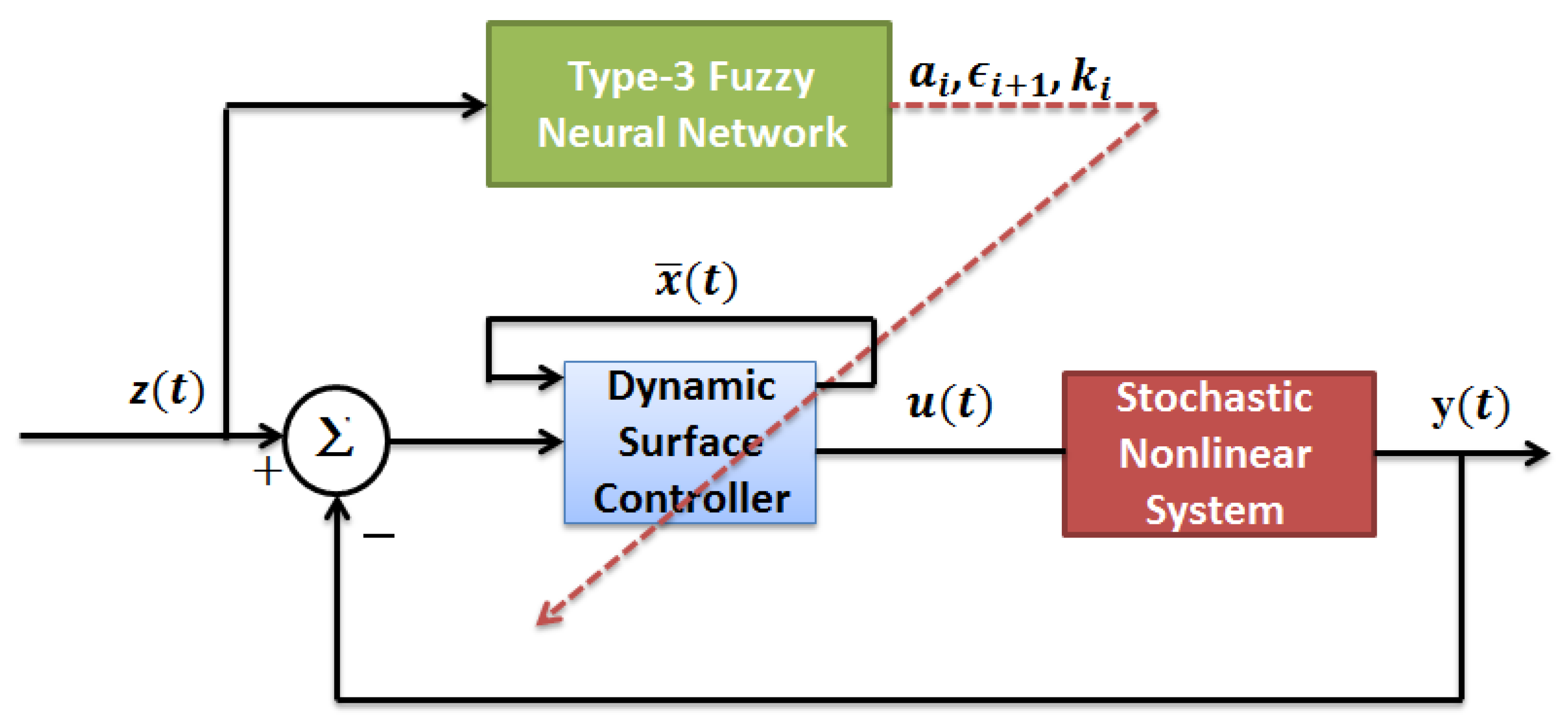
Using the combination of a type-3 fuzzy neural network and a backstepping control method for the first time.

2-

Applying actuator failure to stochastic nonlinear system in a new way.

3-

Ensuring the stability of the control system analytically.

The structure of the article is such that the problem is explained first. Then, the specifications of type-3 fuzzy neural network are presented. The proposed control system is described in detail below. In the simulation section, the performance of the control system is evaluated. Finally. in the conclusion section, all of the research results are expressed.

2. Statement of the Problem

Consider a nonlinear stochastic strict feedback system:

$$\{\begin{array}{c}\begin{array}{c}d{x}_1=\left(g_1{x}_2+f_1\right)dt+{\psi }_{1}d\psi ,\\ ⋮\\ d{x}_i=\left(g_i{x}_{i+1}+f_i\right)dt+{\psi }_{i}d\psi , \end{array}\\ ⋮ \\ \begin{array}{c}d{x}_n=\left(g_{n}u+f_n\right)dt+{\psi }_{n}d\psi , \\ y=x_1, \\ u\left(t\right)=p_{o}v\left(t\right)-d\left[v\right]\left(t\right), \end{array}\end{array}{b}_m\le g_i\le b_M , x={\left[x_1,x_2,\dots ,x_n\right]}^T, 1\le i\le n$$

(1)

where $\psi$ is the standard two-dimensional external motions defined on the probability space (Ω, F, P) with Ω as the sample space, F as a filtration, P as a criterion Probability, and smoothly unknown functions such as below:

$$f_i(·),g_i(·):R^i\times R^{+}\to R, {\psi }_i^T:R^i\times R^{+}\to R^{i\times i},$$

(2)

where

$$f\left(0\right)=0, {\psi }_i^T\left(0\right)=0$$

(3)

It should be noted that in (1), $u$ is the control input or the output of the actuator, which can be exposed to many nonlinear variations, including residuals in the actuator. In conducting this research, and in each step of the stability analysis procedure, a series of definitions, concepts, and lemma will be used, which will be briefly explained as we continue. Consider the following stochastic system:

$$dx=f\left(x,t\right)dt+h\left(x,t\right)d\psi , x={\left[x_1,x_2,\dots ,x_n\right]}^T\in R^n$$

(4)

where $x$ is vector of system state. The following factions are locally Lipchitz functions;

$$f:R^n\times R^{+}\to R^n, h:R^n\times R^{+}\to R^{n\times r},f\left(0,t\right), h\left(0,t\right)=0,\forall t\ge 0$$

(5)

Definition 1.

For each function as follows:

$$V\left(x,t\right)ϵ C^{2,1}\left(R^n\times R^{+},R^{+}\right)$$

(6)

Related to relation (4), the differential actuator L is defined as:

$$LV=\frac{\partial v}{\partial t}+\frac{\partial v}{\partial x}f+\frac{1}{2}Tr\left\{h^T\frac{{\partial }^{2}v}{\partial x^2}h\right\}$$

(7)

The last term of (7) is called an Ito correction. The second order derivative$\frac{{\partial }^{2}v}{\partial x^2}$is the main challenge for the control system designer and the difference between stochastic and deterministic systems is determined in this phrase.

Lemma 1.

Consider a stochastic system (4), and assume that$f\left(x,t\right)$and$h\left(x,t\right)$in their arguments$C^1$,$f\left(0,t\right)$, and$h\left(0,t\right)$are uniformly bounded in$t$. In the following functions:

$$V\left(x,t\right)ϵ C^{2,1}\left(R^n\times R^{+},R^{+}\right), \mu (·),{\mu }_2(·)ϵ K_{\infty }$$

(8)

And there are the constants$a_0>0$,$b_0\ge 0$such that:

$${\mu }_1\left(\left|x\right|\right)\le v\left(x,t\right)\le {\mu }_2\left(\left|x\right|\right), LV\le a_{0}v\left(x,t\right)+b_0$$

(9)

Then the system (4) is bounded in probability.

Lemma 2.

An inequality will also be widely used during the design of the controller and to prove its stability, hence, it is first described as an inequality.

$$xy\le \frac{a^p}{p}[x{]}^p+\frac{1}{q{a}^q}[y{]}^q, \left(p-1\right)\left(q-1\right)=1$$

(10)

Optimal determination of values$p$and$q$is very important. Trial and error methods are commonly used in articles. In this paper, for the first time, we calculate these parameters online using a fuzzy system. This is one of the valuable innovations of this paper.

Lemma 3.

For each continuous function:

$$f\left(x\right):R^n\to R, f\left(0\right)=0,x=[x_1,x_2,\dots .,x_{n]{ }^T}$$

(11)

with always positive functions

$$h_i\left(x_i\right)R\to R^{+}, j=1,2,\dots ,n$$

(12)

There is

$$\left|f\left(x\right)\right|\le {\displaystyle \sum }_{j=1}^n\left|x_j\right|h_j\left(x_j\right)$$

(13)

Executor actuator: analytically, suppose$C_m\left[0,t_E\right]$is a space of uniform continuous fragment functions. For an input$v\left(t\right)$, where$v\left(t\right)\in C_m\left[0,t_E\right]$, the executable actuator is:

$$\begin{array}{c}{F}_r\left[v;u_{-1}\right]\left(0\right)=f_r\left(v\left(0\right),u_{-1}\right)\\ F_r\left[v;u_{-1}\right]\left(t\right)=f_r\left(v\left(t\right),f_r[v;u_{-1}](t_1\right)), t_i<t\le t_{i+1}, 0\le i\le N-1 \end{array}$$

(14)

where,

$$f_1\left(v,u\right)=\max \left(v-r,\min \left(v+r,u\right)\right)$$

(15)

and,

$$0=t_0<t_1<\dots <t_N=t_{E,}$$

(16)

Therefore, there is a fraction in interval$\left[0,t_E\right]$, such that the function$v\left(t\right)$on each of the sub-intervals$\left[t_i,t_{i+1}\right]$is uniform.

Prandtl–Ishlinskii (PI) Waste: It is a nonlinear condition as follows:

$$u\left(t\right)=p_{0}v\left(t\right)-{{\displaystyle \int }}_0^{R}p\left(r\right)f_r\left[v\right]\left(t\right)dr$$

(17)

In which $u\left(t\right)$ is the output of the actuator, $v\left(t\right)$ the input signal to the actuator. $p\left(r\right)$ is the density function, and

$$p_0={{\displaystyle \int }}_0^{R}p\left(r\right)dr$$

(18)

is a constant that depends on the density function $p\left(r\right)$.

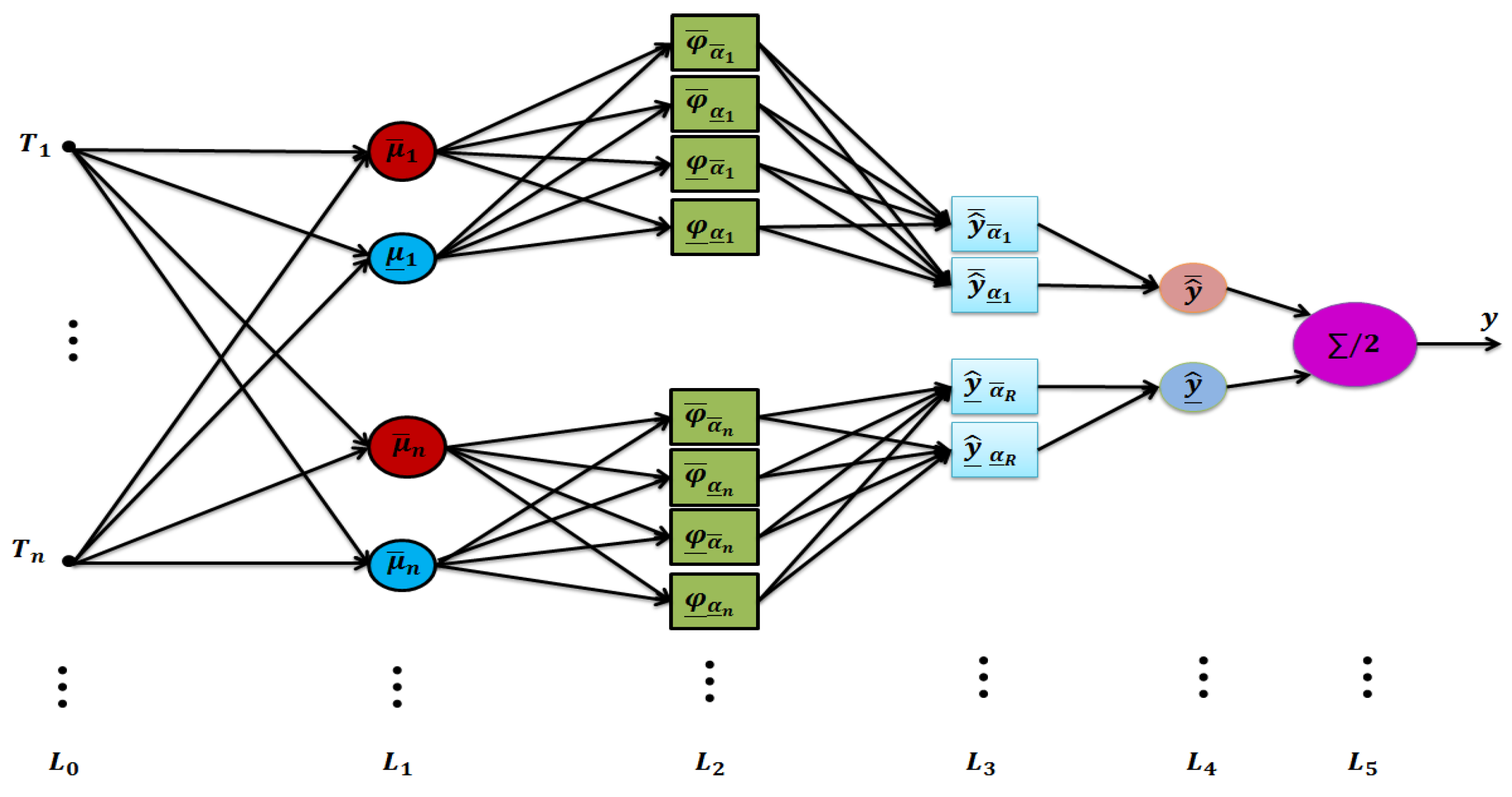
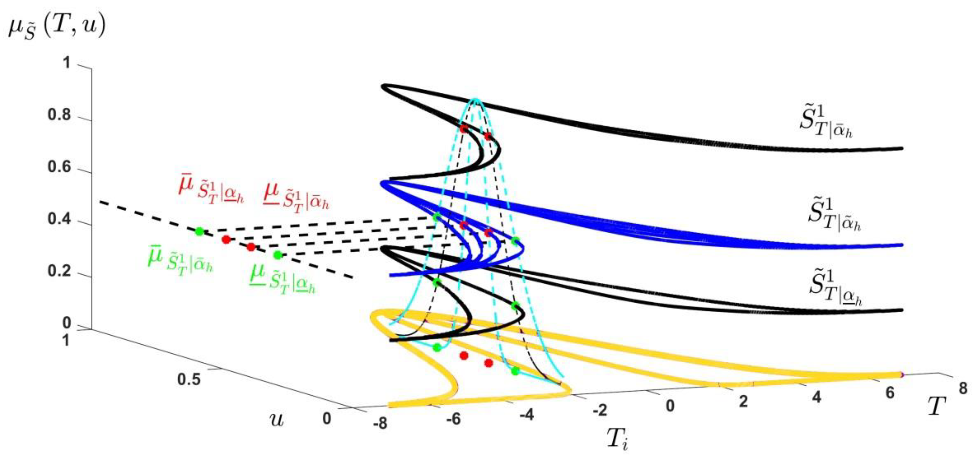
3. Type-3 Fuzzy Neural Network

In this section, the type-3 fuzzy neural network structure (Figure 1) and calculations are presented. The membership degree of type-3 fuzzy sets is calculated as follows:

$${\overline{\mu }}_{{\tilde{S}}_T^j|{\overline{\alpha }}_h}\left(T\right)=\exp \left(-\frac{{\left(T-c_{{\tilde{S}}_T^j|{\overline{\alpha }}_h}\right)}^2}{{\overline{\sigma }}_{{\tilde{S}}_T^j|{\overline{\alpha }}_h}^2}\right),{\overline{\mu }}_{{\tilde{S}}_T^j|{\underset{\_}{\alpha }}_h}\left(T\right)=\exp \left(-\frac{{\left(T-c_{{\tilde{S}}_T^j|{\underset{\_}{\alpha }}_h}\right)}^2}{{\overline{\sigma }}_{{\tilde{S}}_T^j|{\underset{\_}{\alpha }}_h}^2}\right)$$

(19)

$${\underset{\_}{\mu }}_{{\tilde{S}}_T^j|{\overline{\alpha }}_h}\left(T\right)=\exp \left(-\frac{{\left(T-c_{{\tilde{S}}_T^j|{\overline{\alpha }}_h}\right)}^2}{{\underset{\_}{\sigma }}_{{\tilde{S}}_T^j|{\overline{\alpha }}_h}^2}\right),{\underset{\_}{\mu }}_{{\tilde{S}}_T^j|{\underset{\_}{\alpha }}_h}\left(T\right)=\exp \left(-\frac{{\left(T-c_{{\tilde{S}}_T^j|{\underset{\_}{\alpha }}_h}\right)}^2}{{\underset{\_}{\sigma }}_{{\tilde{S}}_T^j|{\underset{\_}{\alpha }}_h}^2}\right)$$

(20)

where, h = 1, …, n, j = 1, 2, $c_{{\tilde{S}}_T^j|{\overline{\alpha }}_h}$ is the mean of MF ${\tilde{S}}_T^j|{\overline{\alpha }}_h$, ${\overline{\sigma }}_{{\tilde{S}}_T^j|{\overline{\alpha }}_h}$, and ${\underset{\_}{\sigma }}_{{\tilde{S}}_T^j|{\overline{\alpha }}_h}$ are the upper and lower standard divisions for ${\tilde{S}}_T^j|{\overline{\alpha }}_h$.

The calculation of upper rule firing at ${\overline{\alpha }}_h$ are as follows:

$${\overline{\phi }}_{{\overline{\alpha }}_h}^1={\overline{\mu }}_{{\tilde{S}}_T^1|{\overline{\alpha }}_h}{\overline{\mu }}_{{\tilde{S}}_P^1|{\overline{\alpha }}_h}{\overline{\mu }}_{{\tilde{S}}_M^1|{\overline{\alpha }}_h},{\overline{\phi }}_{{\overline{\alpha }}_h}^2={\overline{\mu }}_{{\tilde{S}}_T^1|{\overline{\alpha }}_h}{\overline{\mu }}_{{\tilde{S}}_P^1|{\overline{\alpha }}_h}{\overline{\mu }}_{{\tilde{S}}_M^2|{\overline{\alpha }}_h}$$

(21)

$${\overline{\phi }}_{{\overline{\alpha }}_h}^3={\overline{\mu }}_{{\tilde{S}}_T^1|{\overline{\alpha }}_h}{\overline{\mu }}_{{\tilde{S}}_P^2|{\overline{\alpha }}_h}{\overline{\mu }}_{{\tilde{S}}_M^1|{\overline{\alpha }}_h},{\overline{\phi }}_{{\overline{\alpha }}_h}^4={\overline{\mu }}_{{\tilde{S}}_T^1|{\overline{\alpha }}_h}{\overline{\mu }}_{{\tilde{S}}_P^2|{\overline{\alpha }}_h}{\overline{\mu }}_{{\tilde{S}}_M^2|{\overline{\alpha }}_h}$$

(22)

$${\overline{\phi }}_{{\overline{\alpha }}_h}^5={\overline{\mu }}_{{\tilde{S}}_T^2|{\overline{\alpha }}_h}{\overline{\mu }}_{{\tilde{S}}_P^1|{\overline{\alpha }}_h}{\overline{\mu }}_{{\tilde{S}}_M^1|{\overline{\alpha }}_h},{\overline{\phi }}_{{\overline{\alpha }}_h}^6={\overline{\mu }}_{{\tilde{S}}_T^2|{\overline{\alpha }}_h}{\overline{\mu }}_{{\tilde{S}}_P^1|{\overline{\alpha }}_h}{\overline{\mu }}_{{\tilde{S}}_M^2|{\overline{\alpha }}_h}$$

(23)

$${\overline{\phi }}_{{\overline{\alpha }}_h}^7={\overline{\mu }}_{{\tilde{S}}_T^2|{\overline{\alpha }}_h}{\overline{\mu }}_{{\tilde{S}}_P^2|{\overline{\alpha }}_h}{\overline{\mu }}_{{\tilde{S}}_M^1|{\overline{\alpha }}_h},{\overline{\phi }}_{{\overline{\alpha }}_h}^8={\overline{\mu }}_{{\tilde{S}}_T^2|{\overline{\alpha }}_h}{\overline{\mu }}_{{\tilde{S}}_P^2|{\overline{\alpha }}_h}{\overline{\mu }}_{{\tilde{S}}_M^2|{\overline{\alpha }}_h}$$

(24)

The firing of upper rule at α_h, are as follows:

$${\overline{\phi }}_{{\underset{\_}{\alpha }}_h}^1={\overline{\mu }}_{{\tilde{S}}_T^1|{\underset{\_}{\alpha }}_h}{\overline{\mu }}_{{\tilde{S}}_P^1|{\underset{\_}{\alpha }}_h}{\overline{\mu }}_{{\tilde{S}}_M^1|{\underset{\_}{\alpha }}_h},{\overline{\phi }}_{{\underset{\_}{\alpha }}_h}^2={\overline{\mu }}_{{\tilde{S}}_T^1|{\underset{\_}{\alpha }}_h}{\overline{\mu }}_{{\tilde{S}}_P^1|{\underset{\_}{\alpha }}_h}{\overline{\mu }}_{{\tilde{S}}_M^2|{\underset{\_}{\alpha }}_h}$$

(25)

$${\overline{\phi }}_{{\underset{\_}{\alpha }}_h}^3={\overline{\mu }}_{{\tilde{S}}_T^1|{\underset{\_}{\alpha }}_h}{\overline{\mu }}_{{\tilde{S}}_P^2|{\underset{\_}{\alpha }}_h}{\overline{\mu }}_{{\tilde{S}}_M^1|{\underset{\_}{\alpha }}_h},{\overline{\phi }}_{{\underset{\_}{\alpha }}_h}^4={\overline{\mu }}_{{\tilde{S}}_T^1|{\underset{\_}{\alpha }}_h}{\overline{\mu }}_{{\tilde{S}}_P^2|{\underset{\_}{\alpha }}_h}{\overline{\mu }}_{{\tilde{S}}_M^2|{\underset{\_}{\alpha }}_h}$$

(26)

$${\overline{\phi }}_{{\underset{\_}{\alpha }}_h}^5={\overline{\mu }}_{{\tilde{S}}_T^2|{\underset{\_}{\alpha }}_h}{\overline{\mu }}_{{\tilde{S}}_P^1|{\underset{\_}{\alpha }}_h}{\overline{\mu }}_{{\tilde{S}}_M^1|{\underset{\_}{\alpha }}_h},{\overline{\phi }}_{{\underset{\_}{\alpha }}_h}^6={\overline{\mu }}_{{\tilde{S}}_T^2|{\underset{\_}{\alpha }}_h}{\overline{\mu }}_{{\tilde{S}}_P^1|{\underset{\_}{\alpha }}_h}{\overline{\mu }}_{{\tilde{S}}_M^2|{\underset{\_}{\alpha }}_h}$$

(27)

$${\overline{\phi }}_{{\underset{\_}{\alpha }}_h}^7={\overline{\mu }}_{{\tilde{S}}_T^2|{\underset{\_}{\alpha }}_h}{\overline{\mu }}_{{\tilde{S}}_P^2|{\underset{\_}{\alpha }}_h}{\overline{\mu }}_{{\tilde{S}}_M^1|{\underset{\_}{\alpha }}_h},{\overline{\phi }}_{{\underset{\_}{\alpha }}_h}^8={\overline{\mu }}_{{\tilde{S}}_T^2|{\underset{\_}{\alpha }}_h}{\overline{\mu }}_{{\tilde{S}}_P^2|{\underset{\_}{\alpha }}_h}{\overline{\mu }}_{{\tilde{S}}_M^2|{\underset{\_}{\alpha }}_h}$$

(28)

Equations (29)–(36) are formulations of the upper and lower slices of the lower firing rules.

$${\underset{\_}{\phi }}_{{\overline{\alpha }}_h}^1={\overline{\mu }}_{{\tilde{S}}_T^1|{\overline{\alpha }}_h}{\overline{\mu }}_{{\tilde{S}}_P^1|{\overline{\alpha }}_h}{\overline{\mu }}_{{\tilde{S}}_M^1|{\overline{\alpha }}_h},{\underset{\_}{\phi }}_{{\overline{\alpha }}_h}^2={\overline{\mu }}_{{\tilde{S}}_T^1|{\overline{\alpha }}_h}{\overline{\mu }}_{{\tilde{S}}_P^1|{\overline{\alpha }}_h}{\overline{\mu }}_{{\tilde{S}}_M^2|{\overline{\alpha }}_h}$$

(29)

$${\underset{\_}{\phi }}_{{\overline{\alpha }}_h}^3={\overline{\mu }}_{{\tilde{S}}_T^1|{\overline{\alpha }}_h}{\overline{\mu }}_{{\tilde{S}}_P^2|{\overline{\alpha }}_h}{\overline{\mu }}_{{\tilde{S}}_M^1|{\overline{\alpha }}_h},{\underset{\_}{\phi }}_{{\overline{\alpha }}_h}^4={\overline{\mu }}_{{\tilde{S}}_T^1|{\overline{\alpha }}_h}{\overline{\mu }}_{{\tilde{S}}_P^2|{\overline{\alpha }}_h}{\overline{\mu }}_{{\tilde{S}}_M^2|{\overline{\alpha }}_h}$$

(30)

$${\underset{\_}{\phi }}_{{\overline{\alpha }}_h}^5={\overline{\mu }}_{{\tilde{S}}_T^2|{\overline{\alpha }}_h}{\overline{\mu }}_{{\tilde{S}}_P^1|{\overline{\alpha }}_h}{\overline{\mu }}_{{\tilde{S}}_M^1|{\overline{\alpha }}_h},{\underset{\_}{\phi }}_{{\overline{\alpha }}_h}^6={\overline{\mu }}_{{\tilde{S}}_T^2|{\overline{\alpha }}_h}{\overline{\mu }}_{{\tilde{S}}_P^1|{\overline{\alpha }}_h}{\overline{\mu }}_{{\tilde{S}}_M^2|{\overline{\alpha }}_h}$$

(31)

$${\underset{\_}{\phi }}_{{\overline{\alpha }}_h}^7={\overline{\mu }}_{{\tilde{S}}_T^2|{\overline{\alpha }}_h}{\overline{\mu }}_{{\tilde{S}}_P^2|{\overline{\alpha }}_h}{\overline{\mu }}_{{\tilde{S}}_M^1|{\overline{\alpha }}_h},{\underset{\_}{\phi }}_{{\overline{\alpha }}_h}^8={\overline{\mu }}_{{\tilde{S}}_T^2|{\overline{\alpha }}_h}{\overline{\mu }}_{{\tilde{S}}_P^2|{\overline{\alpha }}_h}{\overline{\mu }}_{{\tilde{S}}_M^2|{\overline{\alpha }}_h}$$

(32)

$${\underset{\_}{\phi }}_{{\underset{\_}{\alpha }}_h}^1={\overline{\mu }}_{{\tilde{S}}_T^1|{\underset{\_}{\alpha }}_h}{\overline{\mu }}_{{\tilde{S}}_P^1|{\underset{\_}{\alpha }}_h}{\overline{\mu }}_{{\tilde{S}}_M^1|{\underset{\_}{\alpha }}_h},{\underset{\_}{\phi }}_{{\underset{\_}{\alpha }}_h}^2={\overline{\mu }}_{{\tilde{S}}_T^1|{\underset{\_}{\alpha }}_h}{\overline{\mu }}_{{\tilde{S}}_P^1|{\underset{\_}{\alpha }}_h}{\overline{\mu }}_{{\tilde{S}}_M^2|{\underset{\_}{\alpha }}_h}$$

(33)

$${\underset{\_}{\phi }}_{{\underset{\_}{\alpha }}_h}^3={\overline{\mu }}_{{\tilde{S}}_T^1|{\underset{\_}{\alpha }}_h}{\overline{\mu }}_{{\tilde{S}}_P^2|{\underset{\_}{\alpha }}_h}{\overline{\mu }}_{{\tilde{S}}_M^1|{\underset{\_}{\alpha }}_h},{\underset{\_}{\phi }}_{{\underset{\_}{\alpha }}_h}^4={\overline{\mu }}_{{\tilde{S}}_T^1|{\underset{\_}{\alpha }}_h}{\overline{\mu }}_{{\tilde{S}}_P^2|{\underset{\_}{\alpha }}_h}{\overline{\mu }}_{{\tilde{S}}_M^2|{\underset{\_}{\alpha }}_h}$$

(34)

$${\underset{\_}{\phi }}_{{\underset{\_}{\alpha }}_h}^5={\overline{\mu }}_{{\tilde{S}}_T^2|{\underset{\_}{\alpha }}_h}{\overline{\mu }}_{{\tilde{S}}_P^1|{\underset{\_}{\alpha }}_h}{\overline{\mu }}_{{\tilde{S}}_M^1|{\underset{\_}{\alpha }}_h},{\underset{\_}{\phi }}_{{\underset{\_}{\alpha }}_h}^6={\overline{\mu }}_{{\tilde{S}}_T^2|{\underset{\_}{\alpha }}_h}{\overline{\mu }}_{{\tilde{S}}_P^1|{\underset{\_}{\alpha }}_h}{\overline{\mu }}_{{\tilde{S}}_M^2|{\underset{\_}{\alpha }}_h}$$

(35)

$${\underset{\_}{\phi }}_{{\underset{\_}{\alpha }}_h}^7={\overline{\mu }}_{{\tilde{S}}_T^2|{\underset{\_}{\alpha }}_h}{\overline{\mu }}_{{\tilde{S}}_P^2|{\underset{\_}{\alpha }}_h}{\overline{\mu }}_{{\tilde{S}}_M^1|{\underset{\_}{\alpha }}_h},{\underset{\_}{\phi }}_{{\underset{\_}{\alpha }}_h}^8={\overline{\mu }}_{{\tilde{S}}_T^2|{\underset{\_}{\alpha }}_h}{\overline{\mu }}_{{\tilde{S}}_P^2|{\underset{\_}{\alpha }}_h}{\overline{\mu }}_{{\tilde{S}}_M^2|{\underset{\_}{\alpha }}_h}$$

(36)

The type-reduction procedure from a type-3 fuzzy to a type-2 one, are computed as follows (Figure 2):

$${\overline{\widehat{y}}}_{{\overline{\alpha }}_h}=\frac{{\displaystyle \sum _{l=1}^R{\overline{\phi }}_{{\overline{\alpha }}_h}^l{\overline{\theta }}_l}}{{\displaystyle \sum _{l=1}^R\left({\overline{\phi }}_{{\overline{\alpha }}_h}^l+{\underset{\_}{\phi }}_{{\overline{\alpha }}_h}^l\right)}},{\overline{\widehat{y}}}_{{\underset{\_}{\alpha }}_h}=\frac{{\displaystyle \sum _{l=1}^R{\overline{\phi }}_{{\underset{\_}{\alpha }}_h}^l{\overline{\theta }}_l}}{{\displaystyle \sum _{l=1}^R\left({\overline{\phi }}_{{\underset{\_}{\alpha }}_h}^l+{\underset{\_}{\phi }}_{{\underset{\_}{\alpha }}_h}^l\right)}}$$

(37)

$${\underset{\_}{\widehat{y}}}_{{\overline{\alpha }}_h}=\frac{{\displaystyle \sum _{l=1}^R{\underset{\_}{\phi }}_{{\overline{\alpha }}_h}^l{\underset{\_}{\theta }}_l}}{{\displaystyle \sum _{l=1}^R\left({\overline{\phi }}_{{\overline{\alpha }}_h}^l+{\underset{\_}{\phi }}_{{\overline{\alpha }}_h}^l\right)}},{\underset{\_}{\widehat{y}}}_{{\underset{\_}{\alpha }}_h}=\frac{{\displaystyle \sum _{l=1}^R{\overline{\phi }}_{{\underset{\_}{\alpha }}_h}^l{\underset{\_}{\theta }}_l}}{{\displaystyle \sum _{l=1}^R\left({\underset{\_}{\phi }}_{{\underset{\_}{\alpha }}_h}^l+{\underset{\_}{\phi }}_{{\underset{\_}{\alpha }}_h}^l\right)}}$$

(38)

where, R is the number of rules (here R = 5), and ${\underset{\_}{\theta }}_l$ and ${\overline{\theta }}_l$ are the parameters of the lower and upper of the l-th rule.

The type-reduction procedure from type-2 fuzzy to type-1 one is as follows:

$$\overline{\widehat{y}}=\frac{{\displaystyle \sum _{h=1}^n{\overline{\alpha }}_h{\overline{\widehat{y}}}_{{\overline{\alpha }}_h}}}{{\displaystyle \sum _{h=1}^n\left({\overline{\alpha }}_h+{\underset{\_}{\alpha }}_h\right)}}+\frac{{\displaystyle \sum _{h=1}^n{\underset{\_}{\alpha }}_h{\overline{\widehat{y}}}_{{\underset{\_}{\alpha }}_h}}}{{\displaystyle \sum _{h=1}^n\left({\overline{\alpha }}_h+{\underset{\_}{\alpha }}_h\right)}},\underset{\_}{\widehat{y}}=\frac{{\displaystyle \sum _{h=1}^n{\overline{\alpha }}_h{\underset{\_}{\widehat{y}}}_{{\overline{\alpha }}_h}}}{{\displaystyle \sum _{h=1}^n\left({\overline{\alpha }}_h+{\underset{\_}{\alpha }}_h\right)}}+\frac{{\displaystyle \sum _{h=1}^n{\underset{\_}{\alpha }}_h{\underset{\_}{\widehat{y}}}_{{\underset{\_}{\alpha }}_h}}}{{\displaystyle \sum _{h=1}^n\left({\overline{\alpha }}_h+{\underset{\_}{\alpha }}_h\right)}}$$

(39)

The output $\widehat{y}$ is computed as:

$$\widehat{y}=\frac{\overline{\widehat{y}}+\underset{\_}{\widehat{y}}}{2}$$

(40)

The type-3 fuzzy neural network parametric learning process can be seen in Appendix A.

4. Controller Design

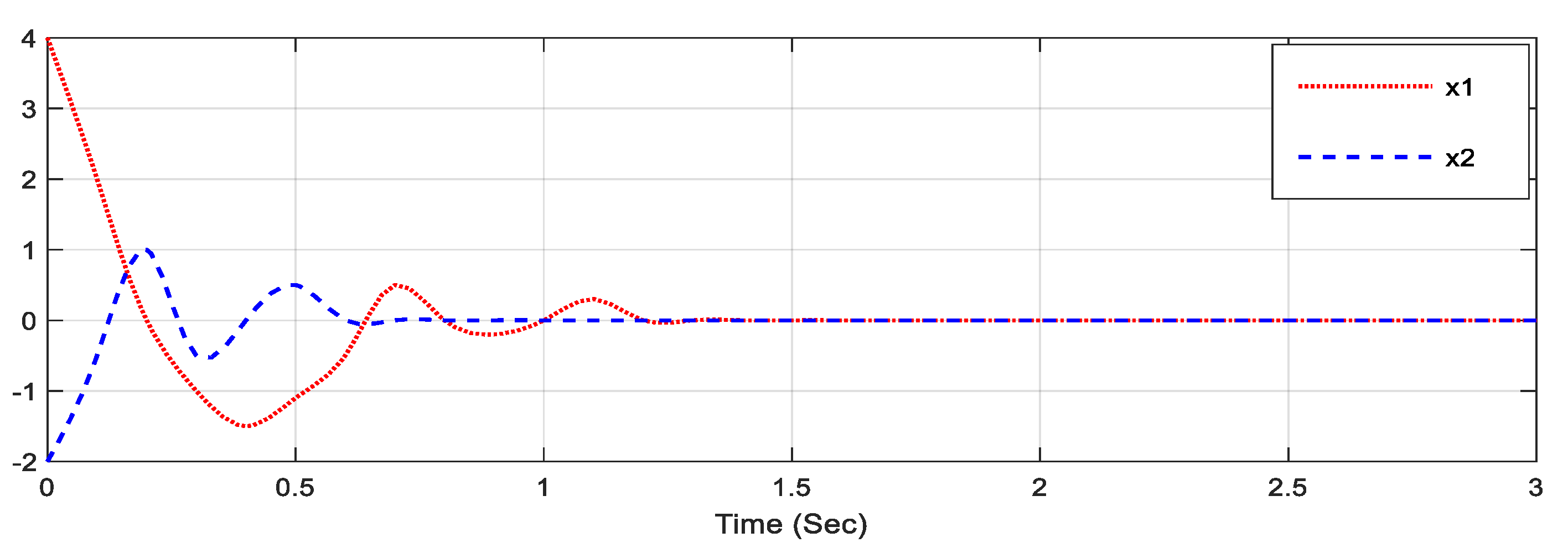
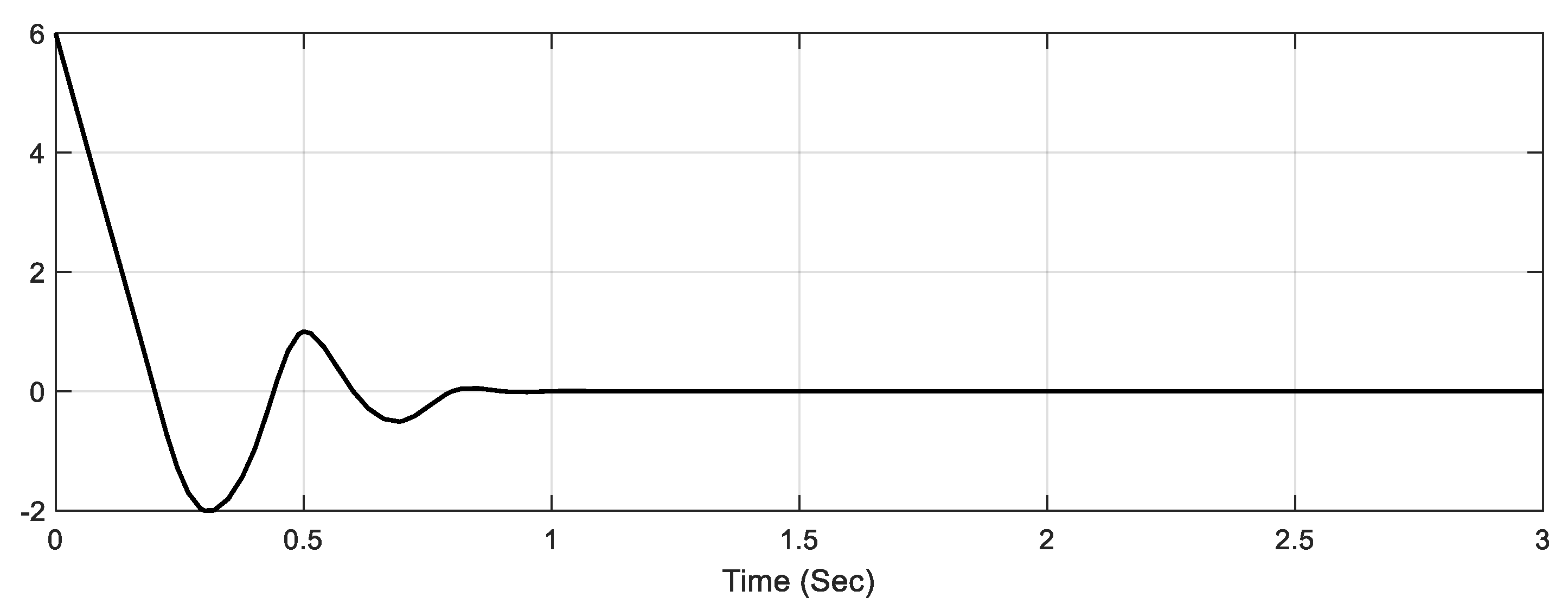
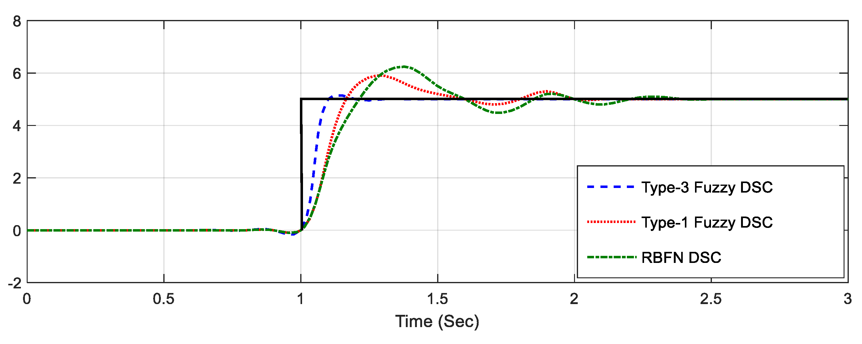
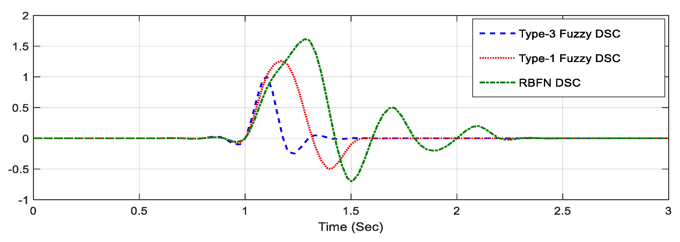
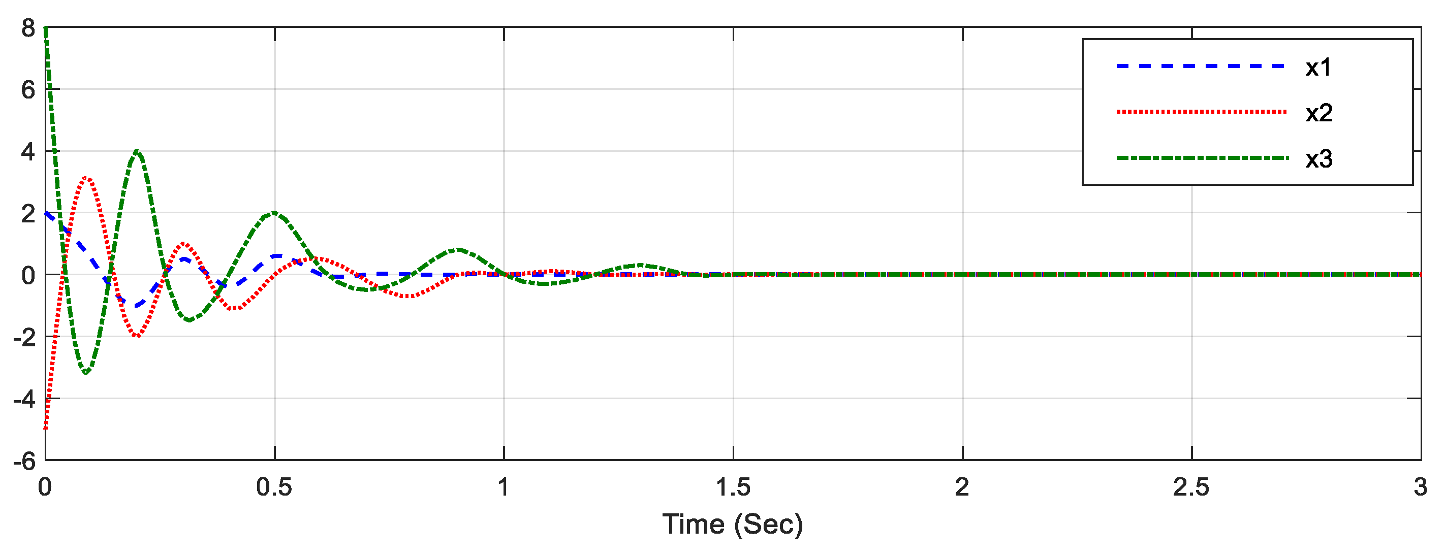
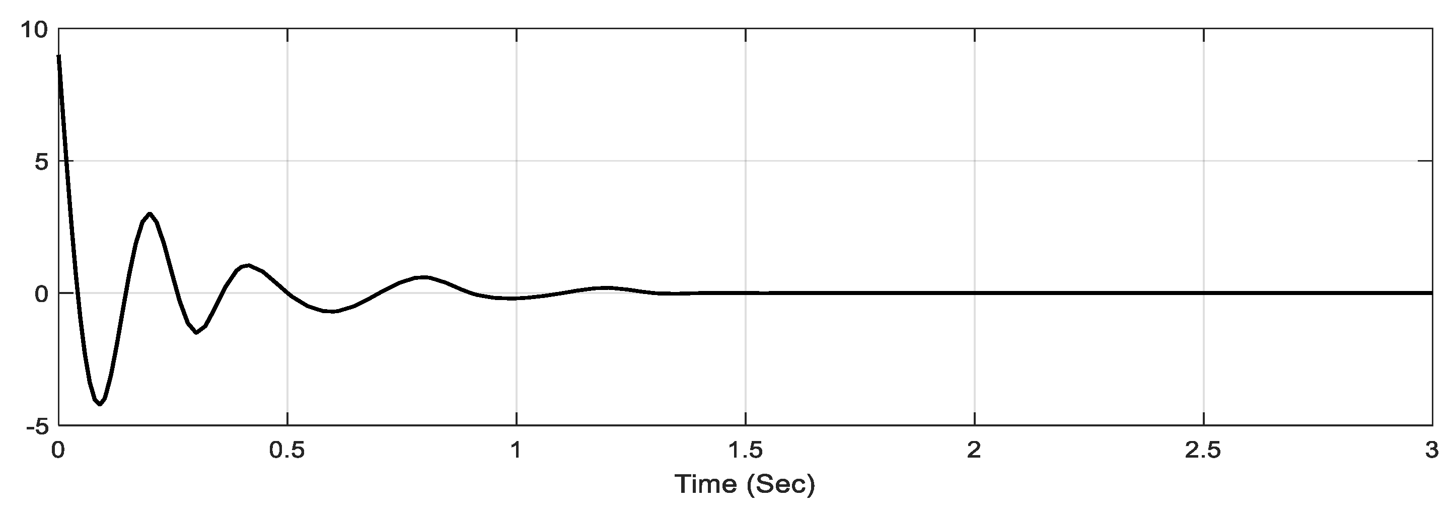
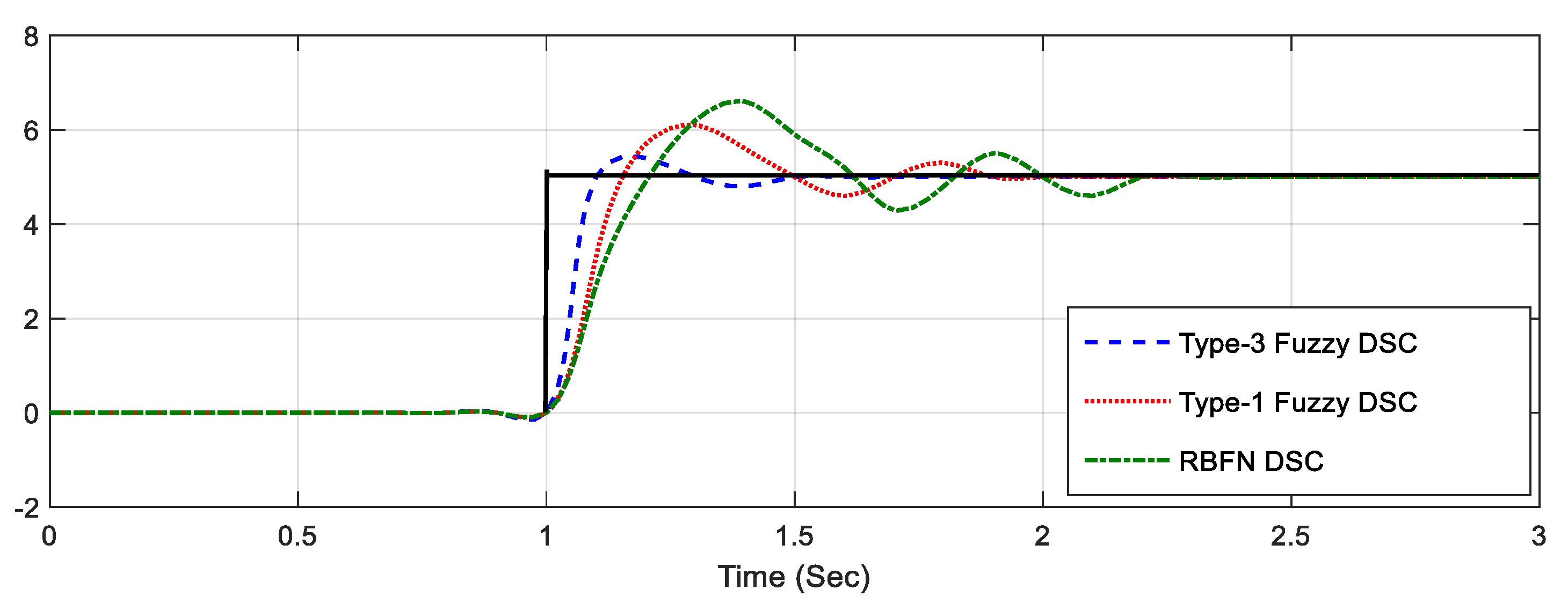
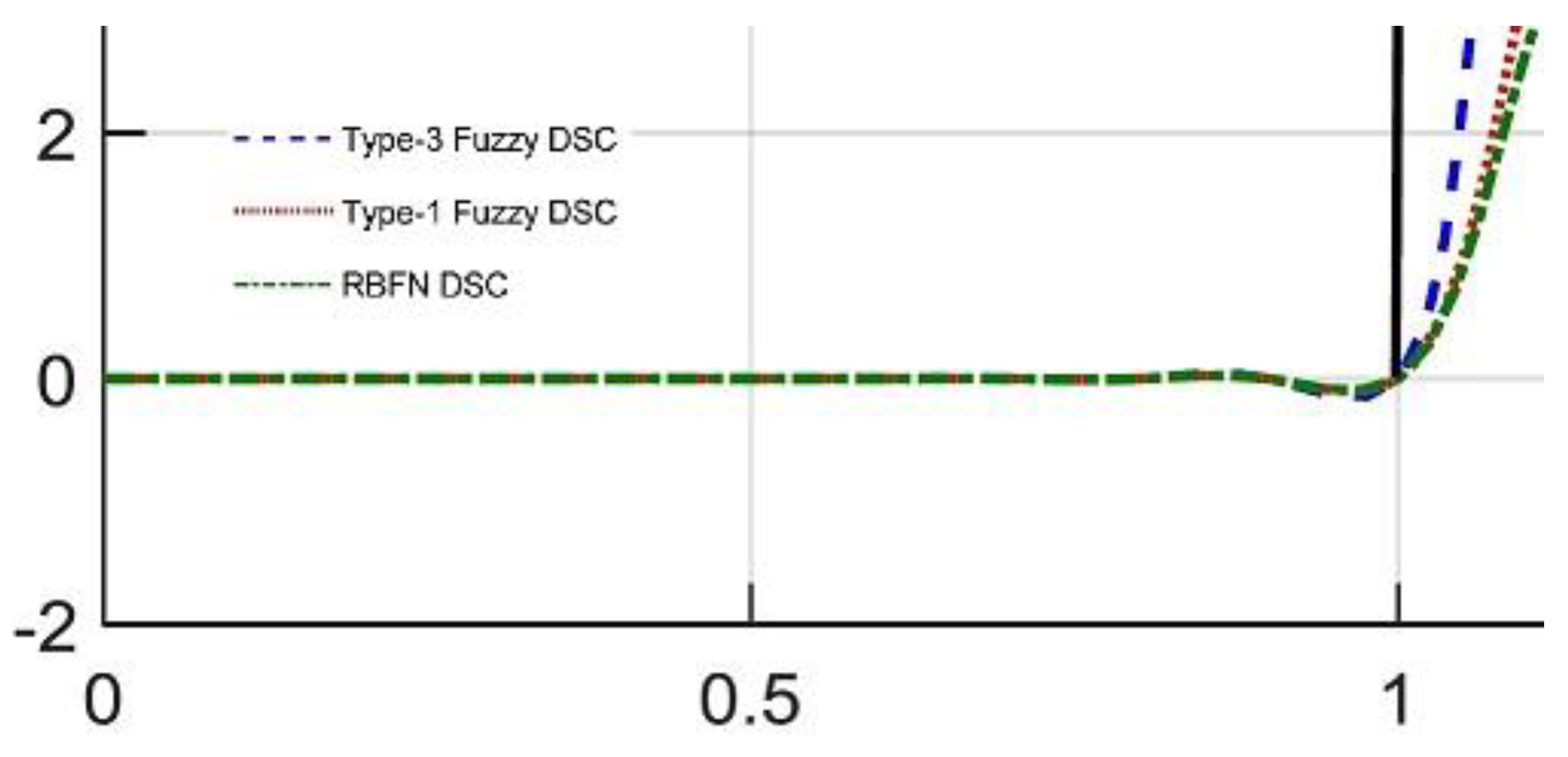
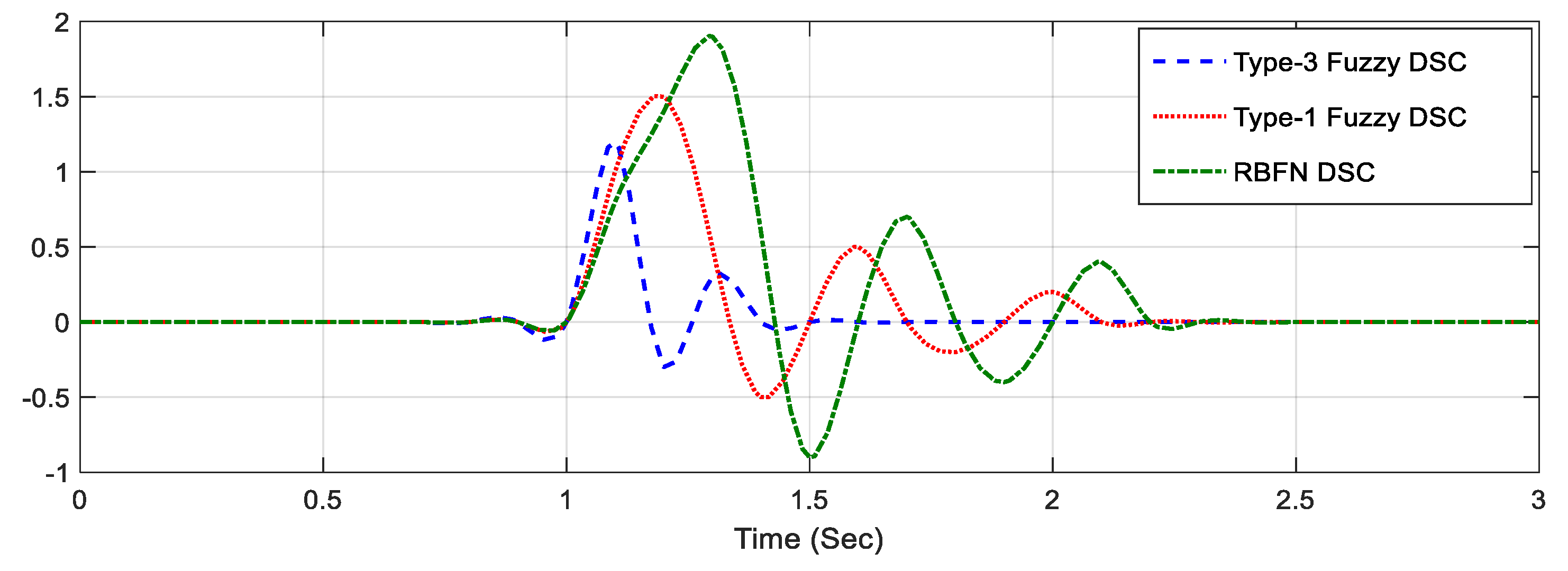
As presented in the literature review, an approach for the stabilization of stochastic nonlinear systems is presented in the form of strict feedback, which is based on the backstepping design technique and neural networks. The present method is an extension of the method proposed in [5]. The differences between our work and the aforementioned work are as follows: replacing the backstepping design method by using the dynamic surface control (DSC) design, and the use of a type-3 fuzzy system instead of a radial base function neural network (RBFN). Numerous articles have proven the ability and accuracy of type-3 fuzzy systems compared to other computational intelligence tools. Finally, the proposed design method will be used to investigate the occurrence of PI waste in the actuator. This method is based on a multi-step recursive design algorithm that will be described below. Consider the strict feedback stochastic nonlinear system (17), then for each $i$ step, an error surface ($S_i$), as follows:

$$S_i=x_i-z_i, 1\le i\le n, z_1=y_r$$

(41)

where $S_i$ is the i-th error surface, $x_i$ is the i-th state, and $z_i$ is the i-th desired state for the system. The proposed design procedure consists of n sequential step calculations. A virtual control input ${\overline{x}}_{i+1}$ for each step is defined as follows:

$$\begin{array}{c}{\overline{x}}_{i+1}=-k_i{S}_i-\frac{1}{2a_i}{S}_i^3\widehat{\theta }{\zeta }_i^T\left(z_i\right){\zeta }_i\left(z_i\right), 1\le i\le n, z_i=\left[\breve{x_i},\widehat{\theta }\right], \breve{x_i}=\left[x_1,\dots ,x_i\right]\\ v=\overline{x_{n+1}}=-k_n{S}_n-\frac{1}{2a_n}{S}_n^3\widehat{\theta }{\zeta }_i^T\left(z_n\right){\zeta }_n\left(z_n\right) \end{array}$$

(42)

where $k_i$ and $a_i$ are the design parameters (calculated by a type-3 fuzzy system), and ${\zeta }_i\left(z_i\right)$ are the type-3 fuzzy membership functions in the first layer of the type-3 fuzzy neural network. An estimation of $\theta$ is shown by $\widehat{\theta }$. The virtual control input is passed through a low-pass filter in order to obtain the desired value of the next step mode.

$${ϵ}_{i+1}{\dot{z}}_{i+1}+z_{i+1}={\overline{x}}_{i+1} , 1\le i\le n-1$$

(43)

In (21), ${ϵ}_{i+1}$ is design parameter (calculated by type-3 fuzzy system). The i-th filter error is as follows:

$$y_i=z_i-{\overline{x}}_i=-{ϵ}_i{\dot{z}}_i$$

(44)

The derivative of (22) is as follows:

$$d{y}_i=\left(\frac{y_i}{{ϵ}_i}+B_i\left(s_i,{\zeta }_i,y_i,\theta ,x_i,x_i\right)\right)dt+G_i\left(s_i,{\zeta }_i,y_i,\theta ,x_i,x_i\right)d\psi$$

(45)

where $B_i(.)$ and $G_i(.)$ are smooth and continuous functions, with maximums of $M_i$ and $N_i$, respectively. The adaptation law to update the parameters of the type-3 fuzzy neural network is as follows:

$$\widehat{\theta }={\displaystyle \sum }_{j=1}^n\frac{\lambda }{2a_j^2}{S}_J^6{\zeta }_j^T\left(z_j\right){\zeta }_j\left(z_j\right)-k_0\widehat{\theta }$$

(46)

The block diagram of the proposed control system is shown in Figure 3.

As shown in Figure 3, the dynamic surface control (DSC) is the main controller that needs to be configured. In previous studies that have been carried out, the parameters of this controller were usually calculated by trial and error or with prior knowledge, but in this article, we use the type-3 fuzzy neural network to calculate the aforementioned parameters. Online tunning of control system parameters is very important, especially in systems with high nonlinearity dynamics or stochastic systems, such as in [25,26].

5. Simulations

In this section, to show the efficiency of the proposed method, two stochastic nonlinear dynamic systems will be controlled and the results will be depicted.

Example 1.

Consider the following second-order stochastic nonlinear system.

$$\{\begin{array}{c}d{x}_1=\left(\left(1+x_1^2\right)x_2+x_{1}sin\left(x_1\right)\right)dt+x_1^{3}d\psi \\ d{x}_2=\left(\left(2+\frac{x_2^2}{1+x_1^2}\right)u+x_1{x}_2^2\right)dt+\left(1+sin\left(x_1\right)\right)x_{2}d\psi \\ y=x_1 \end{array}$$

(47)

where$x_1$and$x_2$are the states of the system,$u$is the input of the system (control signal), and$y$is the system’s output. Figure 4 shows the simulation result of Example 1 and the performance of the proposed control system (dynamic surface control with a type-3 fuzzy neural network) for the convergence of both system states.

The control signal generated by the proposed control system for the convergence of the states in Figure 4 is shown in Figure 5.

For further evaluation and analysis, the proposed control method is compared with the other two methods. In this scenario, the system output is supposed to rise from 0 to 5 after 1 s. One method is a dynamic surface control based on type-1 fuzzy system, and the other is based on radial basis function neural network. Figure 6 shows the result of this comparison.

The control signals generated by all three controllers in Figure 6 are shown in Figure 7.

It can be seen from Figure 4, Figure 5, Figure 6 and Figure 7 that the proposed control system has a good performance and has been able to manage the states (output) of the controlled system in less than 1 s. Additionally, comparison with the other two controllers (type-1 fuzzy and RBFN) shows the high speed and accuracy of the type-3 fuzzy. It can be seen from Figure 7 that the control cost (control signal peak) in the type-3 fuzzy is much lower than the other cases. In the following, a more complex system (48) is introduced, and the performance of the control system for this system (Example 2) is challenged.

Example 2.

Consider the following third-order stochastic nonlinear system.

$$\{\begin{array}{c}d{x}_1=\left(\left(0.3+x_1^2\right)x_2-0.8sin\left(x_1\right)\right)dt+x_{1}sin\left(x_1\right)d\psi \\ d{x}_2=\left(\left(1+x_2^2\right)x_3-x_2-0.5x_2^3-x_1^3-\sqrt{x_1}\right)dt+x_{1}cos\left(x_2\right)d\psi \\ \begin{array}{c}d{x}_3=\left(\left(1.5+sin\left(x_1{x}_2\right)\right)x_3-0.5x_3-\frac{1}{3}{x}_3^2-x_2^2{x}_3-\frac{x_1}{1+x_1^2}\right)dt+3x_1{e}^{x_2^2}d\psi \\ y=x_1 \end{array} \end{array}$$

(48)

where$x_1$and$x_2$are the states of the system,$u$is the input of the system (control signal), and$y$is the system’s output. This system (48) has three states, and the proposed control system has been able to converge all of them very well (Figure 8).

As shown in Figure 9, the control signal converges the system in less than 1.5 s. As in Example 1, here the performance of the proposed control system is compared with the other two methods, and the results are shown in Figure 10.

It is seen in Figure 10 that the proposed control method (DSC based on a type-3 fuzzy system) manages and controls the system (48) in less than 0.5 s, while the RBFN-based method takes more than 1 s. The control signal of all three controllers for the aforementioned operation is shown in Figure 12.

As can be seen from Figure 8, Figure 9, Figure 10, Figure 11 and Figure 12, the proposed control method has been able to handle a nonlinear and complex random system (48) well and control it in less than 1 s. Figure 10 shows that the DSC based on the type-3 fuzzy system touches the desired value for the first time in less than 0.1 s, and that the overshoot percentage is less than 6%. Additionally, Figure 11 shows a close view of Figure 10 when the step is applied. Figure 12, which shows the control signal of all three controllers, clearly shows the fast response of the proposed method with the lowest control cost. The swirling domain of the proposed controller control signal is much lower than the RBFN DSC and type-1 fuzzy DSC methods, and its response is about 0.6 s faster than other two mentioned methods.

6. Conclusions

In this paper, an innovative control method for stochastic nonlinear systems is presented. In this method, for the first time, a new type-3 fuzzy system in the framework of neural networks (commonly called a type-3 fuzzy neural network) was used to adjust the dynamic surface control method. The class of stochastic nonlinear systems was considered as strict feedback with Prandtl–Ishlinskii (PI) waste, which includes a wide range of real-world systems. The proposed control system was set up to detect changes in less than 1 s, and to generate the appropriate signal immediately. To evaluate the proposed method, two common and widely used systems are simulated, and the results show the high efficiency and accuracy of the proposed control system. Additionally, to compare with other methods, two methods (a type-1 fuzzy system and RBFN) were compared with the proposed method, which testifies to the superiority of the proposed method both in terms of speed and accuracy and in terms of minimum control cost (minimum overshoot).

References

1. Vaiana, N.; Sessa, S.; Marmo, F.; Rosati, L. A class of uniaxial phenomenological models for simulating hysteretic phenomena in rate-independent mechanical systems and materials. Nonlinear Dyn. 2018, 93, 1647–1669. [Google Scholar] [CrossRef]
2. Vaiana, N.; Sessa, S.; Rosati, L. A generalized class of uniaxial rate-independent models for simulating asymmetric mechanical hysteresis phenomena. Mech. Syst. Signal Process. 2021, 146, 106984. [Google Scholar] [CrossRef]
3. Aguirre, G.; Janssens, T.; Brussel, H.V.; Al-Bender, F. Asymmetric-hysteresis compensation in piezoelectric actuators. Mech. Syst. Signal Process. 2012, 30, 218–231. [Google Scholar] [CrossRef]
4. Borisov, A.; Bosov, A.; Miller, A. Optimal Stabilization of Linear Stochastic System with Statistically Uncertain Piecewise Constant Drift. Mathematics 2022, 10, 184. [Google Scholar] [CrossRef]
5. Bashkirtseva, I. Controlling Stochastic Sensitivity by Feedback Regulators in Nonlinear Dynamical Systems with Incomplete Information. Mathematics 2021, 9, 3229. [Google Scholar] [CrossRef]
6. Tavoosi, J.; Shirkhani, M.; Abdali, A.; Mohammadzadeh, A.; Nazari, M.; Mobayen, S.; Asad, J.H.; Bartoszewicz, A. A New General Type-2 Fuzzy Predictive Scheme for PID Tuning. Appl. Sci. 2021, 11, 10392. [Google Scholar] [CrossRef]
7. Wang, J.; Xu, C.; Tavoosi, J. A Novel Nonlinear Control for Uncertain Polynomial Type-2 Fuzzy Systems (Case Study: Cart-Pole System). Int. J. Uncertain. Fuzziness Knowl.-Based Syst. 2021, 29, 753–770. [Google Scholar] [CrossRef]
8. Mohammadi, F.; Mohammadi-ivatloo, B.; Gharehpetian, G.B.; Ali, M.H.; Wei, W.; Erdinç, O.; Shirkhani, M. Robust Control Strategies for Microgrids: A Review. IEEE Syst. J. 2021, 1–12. [Google Scholar] [CrossRef]
9. Wang, M.; Wang, Z.; Dong, H.; Han, Q.L. A Novel Framework for Backstepping-Based Control of Discrete-Time Strict-Feedback Nonlinear Systems with Multiplicative Noises. IEEE Trans. Autom. Control 2021, 66, 1484–1496. [Google Scholar] [CrossRef]
10. Zhang, H.; Zhang, X.; Bu, R. Radial Basis Function Neural Network Sliding Mode Control for Ship Path Following Based on Position Prediction. J. Mar. Sci. Eng. 2021, 9, 1055. [Google Scholar] [CrossRef]
11. Niu, B.; Li, H.; Zhang, Z.; Li, J.; Hayat, T.; Alsaadi, F.E. Adaptive Neural-Network-Based Dynamic Surface Control for Stochastic Interconnected Nonlinear Nonstrict-Feedback Systems with Dead Zone. IEEE Trans. Syst. Man Cybern. Syst. 2019, 49, 1386–1398. [Google Scholar] [CrossRef]
12. O’Hara, J.M.; Jolly, J.C.K.; Reynold, C.E.; Mantis, N.J. Localization of non-linear neutralizing B cell epitopes on ricin toxin’s enzymatic subunit (RTA). Immunol. Lett. 2014, 158, 7–13. [Google Scholar] [CrossRef] [PubMed] [Green Version]
13. Labiod, S.; Guerra, T.M. Adaptive Fuzzy Control for Multivariable Nonlinear Systems with Indefinite Control Gain Matrix and Unknown Control Direction. IFAC-PapersOnLine 2020, 53, 8019–8024. [Google Scholar] [CrossRef]
14. Fei, J.; Fang, Y.; Yuan, Z. Adaptive Fuzzy Sliding Mode Control for a Micro Gyroscope with Backstepping Controller. Micromachines 2020, 11, 968. [Google Scholar] [CrossRef]
15. Wu, G.Q.; Song, S.M.; Sun, J.N. Finite-Time Dynamic Surface Antisaturation Control for Spacecraft Terminal Approach Considering Safety. J. Spacecr. Rocket. 2018, 55, 1430–1443. [Google Scholar] [CrossRef]
16. Ma, Z.; Ma, H. Adaptive Fuzzy Backstepping Dynamic Surface Control of Strict-Feedback Fractional-Order Uncertain Nonlinear Systems. IEEE Trans. Fuzzy Syst. 2020, 28, 122–133. [Google Scholar] [CrossRef]
17. Hu, J.; Zhang, P.; Kao, Y.; Liu, H.; Chen, D. Sliding mode control for Markovian jump repeated scalar nonlinear systems with packet dropouts: The uncertain occurrence probabilities case. Appl. Math. Comput. 2019, 362, 124574. [Google Scholar] [CrossRef]
18. Sui, S.; Chen, C.L.P.; Tong, S. Neural-Network-Based Adaptive DSC Design for Switched Fractional-Order Nonlinear Systems. IEEE Trans. Neural Netw. Learn. Syst. 2021, 32, 4703–4712. [Google Scholar] [CrossRef]
19. Sheng, Z.; Lin, C.; Chen, B.; Wang, Q.G. An asymmetric Lyapunov-Krasovskii functional method on stability and stabilization for T-S fuzzy systems with time delay. IEEE Trans. Fuzzy Syst. 2021, 1. [Google Scholar] [CrossRef]
20. Min, H.; Xu, S.; Zhang, Z. Adaptive Finite-Time Stabilization of Stochastic Nonlinear Systems Subject to Full-State Constraints and Input Saturation. IEEE Trans. Autom. Control 2021, 66, 1306–1313. [Google Scholar] [CrossRef]
21. Wang, J.; Liu, Z.; Zhang, Y.; Chen, C.L.P.; Lai, G. Adaptive Neural Control of a Class of Stochastic Nonlinear Uncertain Systems With Guaranteed Transient Performance. IEEE Trans. Cybern. 2020, 50, 2971–2981. [Google Scholar] [CrossRef] [PubMed]
22. Homayoun, B.; Arefi, M.M.; Vafamand, N. Robust adaptive backstepping tracking control of stochastic nonlinear systems with unknown input saturation: A command filter approach. Int. J. Robust Nonlinear Control 2020, 30, 3296–3313. [Google Scholar] [CrossRef]
23. Liu, H.; Li, X.; Liu, X.; Wang, H. Backstepping-based decentralized bounded-H∞ adaptive neural control for a class of large-scale stochastic nonlinear systems. J. Frankl. Inst. 2019, 356, 8049–8079. [Google Scholar] [CrossRef]
24. Mohammadzadeh, A.; Castillo, O.; Band, S.S.; Mosavi, A. A Novel Fractional-Order Multiple-Model Type-3 Fuzzy Control for Nonlinear Systems with Unmodeled Dynamics. Int. J. Fuzzy Syst. 2021, 23, 1633–1651. [Google Scholar] [CrossRef]
25. Al-Bender, F.; Symens, W.; Swevers, J.; Brussel, H.V. Theoretical analysis of the dynamic behavior of hysteresis elements in mechanical systems. Int. J. Non-Linear Mech. 2004, 39, 1721–1735. [Google Scholar] [CrossRef]
26. Vaiana, N.; Sessa, S.; Marmo, F.; Rosati, L. Nonlinear dynamic analysis of hysteretic mechanical systems by combining a novel rate-independent model and an explicit time integration method. Nonlinear Dyn. 2019, 98, 2879–2901. [Google Scholar] [CrossRef]
Figure 1. The structure of the type-3 fuzzy neural network.
Mathematics 10 01406 g001
Figure 2. A view of the type-3 MF horizontal slices.
Mathematics 10 01406 g002
Figure 3. Block diagram of the proposed control system.
Mathematics 10 01406 g003
Figure 4. The states of the system (47).
Mathematics 10 01406 g004
Figure 5. The control signal.
Mathematics 10 01406 g005
Figure 6. Comparison of dynamic surface control performance based on the type-3 fuzzy system, type-1 fuzzy system, and RBFN.
Mathematics 10 01406 g006
Figure 7. The control signals of the three controllers in Figure 6.
Mathematics 10 01406 g007
Figure 8. The control signal generated by the proposed control system is shown in Figure 9.
Mathematics 10 01406 g008
Figure 9. The control signal.
Mathematics 10 01406 g009
Figure 10. Comparison of dynamic surface control performance based on the type-3 fuzzy system, type-1 fuzzy system and RBFN.
Mathematics 10 01406 g010
Figure 11. A closer view of Figure 10.
Mathematics 10 01406 g011
Figure 12. The control signals of the three controllers in Figure 10.
Mathematics 10 01406 g012
Publisher’s Note: MDPI stays neutral with regard to jurisdictional claims in published maps and institutional affiliations.