1. Introduction
In contrast to the traditional global methods, local methods give the solution of a partial differential equation at an arbitrary point of its domain directly, instead of extracting the response value at this point from the whole field solution. These methods are based on probabilistic interpretations of certain partial differential equations. The relationship between stochastic processes and parabolic and elliptic differential equations was demonstrated a long time ago by Lord Rayleigh [
1] and Courant [
2], respectively. The development of the probabilistic methods is based on the It
calculus, properties of It
diffusion processes, and Monte Carlo simulations. The theoretical considerations supporting the probabilistic methods involve random processes and stochastic integrals. An elaborate presentation of this framework can be found in [
3,
4,
5,
6] and the references cited therein. The main idea of these approaches concerns boundary value problems in bounded domains: A probabilistic manner to interpret the value of the solution of the boundary value problem at a specific point
x is to consider a plethora of stochastic trajectories, emanating from
x and driven by a drift and diffused by a Wiener process connected both directly with the coefficients of the differential operator under investigation. These trajectories travel inside the bounded domain and cross the boundary in finite time. Averaging the values of the field at the boundary hitting points (thus evoking the boundary condition of the problem) gives a very good estimation of the sought solution of the boundary value problem. In exterior domains, the situation changes drastically since the unboundedness of the domain does not provide any reason justifying the aforementioned boundary hitting in finite time. This is the main reason why no systematic probabilistic attempts had been made to face boundary value problems in unbounded domains.
Recently, the probabilistic interpretation of boundary value problems in exterior domains has been reestablished appropriately in [
7]. The main effort in that work was to force the trajectories emanating from the point
x and travelling inside the infinite domain
D to hit the boundary
in finite time. Without special treatment, the generated trajectories have a strong probability to travel to infinity without hitting the boundary of the domain. Actually, even if some paths cross the boundary, their travel time could be very large, creating strong difficulties to the application of the Monte Carlo simulation. The monitoring of the trajectories is accomplished by selecting appropriately a set of attracting or repulsive points
, which constitute irregular points for the stochastic process. This actually is not enough since the orientation of the trajectories towards or away from these singular points is simultaneously guaranteed by the repulsive lateral surfaces of several cones
having as vertexes the singular points. These cones are repulsive since on the lateral surfaces the driving terms of the stochastic processes obtain infinite values. The process of the directivity of the stochastic paths inside the cones under discussion has been presented extensively in [
7] but we focus here on the fact that the monitoring of the curves is mainly accomplished via suitable stochastic differential equations with driving terms generated by the eigen-solutions of the Laplace operator in local (associated to the cones) spherical coordinates. The point is that under this directionality, the generated trajectories hit (for the first time) the boundary
in finite time. All these paths are gathered and exploited as follows: The points of the boundary on which the first exit occurs—the traces of the trajectories on the boundary—are selected and offer a set of points on which the average of the values of the boundary data of the boundary value problem is calculated thus formatting a first accumulation term. In addition, on every trajectory a stochastic integral is calculated where the integrand is the inhomogeneous term of the underlying differential equation. The mean value of these integrals over the large number of trajectories forms a second accumulator which is superposed to the first one, (this second term is absent in the case of a homogeneous differential equation) leading to the construction of an extended mean value term. When the number of the trajectories increases, the aforementioned total mean value converges to the corresponding probabilistic expectation value of the underlying fields, which in turn coincides with the value sought from the beginning of the solution of the boundary value problem at the starting point
x. The description above refers rather to the Dirichlet problem, which is the main subject of investigation in the present work but similar arguments are encountered in the Neumann boundary value problem [
8,
9]. One of the main advantages of the probabilistic approach is that it is based on very stable and accurate Monte Carlo simulations. In [
7], the above methodology has been developed and applied mainly in the exterior Laplace boundary value problem, referring so to potential functions.
In the present work, a probabilistic framework handling the acoustic scattering problem is developed. More precisely, we consider the exterior Dirichlet boundary value problem involving the Helmholtz operator, without restriction on the wavenumber. It worth mentioning that working with stochastic trajectories that stemmed from the Helmholtz equation itself diversifies qualitatively the stochastic framework by offering two alternative stochastic differential regimes, referring to preselected outgoing or ingoing wave propagation. In brief terms, this deviation is due to the nature of the driving terms which govern, in conjunction with the Wiener process, the topology of the stochastic curves. These driving terms are built in the form
—where
h belongs to the kernel of the Helmholtz operator—and are responsible for the probabilistic conditioning. They are expressed in terms of spherical local coordinates inside the cones
. The crucial remark is that two alternatives emerge: When the generating function is selected to be equal to
, where
stands for the spherical Bessel function of second kind and order
m, the trajectories are forced to move inwardly, from the observation point towards the scatterer’s region. This behavior is reminiscent of the stochastic design encountered in [
7]. In contrast to that, when the selection is set to
, involving now the spherical Bessel functions of first kind
, the stochastic curves present an opposite behavior. More precisely, most of the trajectories emanating from
x move fast away outwards, hitting the exterior cup of the cone, which represents a portion of the measurement region located at the near field or far field regime, depending on the measurement status and the subsequent narrowness (the angle of the cone is just the first positive root of the Legendre polynomial
) of the cone. The two situations above can be melted by selecting the radial part of the driving function
to be a combination of the spherical Bessel functions:
. Choosing suitably the coefficient
, it is feasible to settle a stochastic framework assuring equipartition of stochastic experiments in two directions: The outgoing trajectories hitting the measurement region and revealing the contribution of the data and the ingoing trajectories hitting the scatterer and activating the boundary condition. This is an efficient manner to acquire a stochastic representation for the acoustic field
u at the observation point
x, which constitutes simultaneously the emanation point of the stochastic experiments. Actually, the description above settles the framework of the direct scattering problem.
In the realm of the inverse scattering problem, which is the cornerstone of the current work, the common issue with the settlement above is the invocation of the radial function , establishing the aforementioned equipartition of the stochastic experiments. The essential structural difference stems from the simple argument that a representation scheme involving three separate terms (the value of the acoustic field u at the starting point x and the expectation values of the field on both detached portions of the cone with the scatterer and the data region) is an underdetermined scheme. To diminish the unknowns of the problem, we do not apply the stochastic analysis to the acoustic field itself, but to the solenoidal vector Helmholtz equation solution and potentially to the scalar Helmholtz equation solution . These functions merit the principal property of vanishing at the starting point x, leaving alone among the terms of the aforementioned triple, the tag of war between the expectation values over the data region and the scatterer’s surface, where the boundary condition prevails. Following a sampling process, in the case that the vertex of the cone detects the scatterer’s surface points, a functional measuring the balance between the abovementioned measurement term and the boundary condition attains minimum values and quantifies the inversion.
The structure of the work is developed as follows: In
Section 2, the mathematical principles of the scattering problem are briefly presented. In
Section 3, the stochastic differential equations that stemmed from the boundary value problem under discussion are constructed and the suitably layered conical regions serving as the domains of the stochastic processes are confined. The probabilistic analysis of the subsequent stochastic differential system is also developed. This analysis focuses on the analytical investigation of a priori estimates concerning all the involved probabilities of hitting the several surface portions of the conical structures. Especially in
Section 3.2, three separate stochastic representations of the scattered field are provided based on outgoing, ingoing and mixed-type propagating stochastic trajectories. Special attention has been paid to the third case constituting a stochastic representation, embodying, in an equipartitioned manner, the contribution of the data region as well as of the scatterer’s surface. These representations and mainly the third one constitute alternative probabilistic representations of the scattered field and could be considered as the stochastic analogue of the well known classical integral representations, produced on the basis of Green’s theorem. In
Section 4, some crucial parameters of the stochastic implementation are investigated as far as their numerical implementation is concerned. The solution of the inverse scattering problem from convex scatterers on the basis of exploiting stochastically far field data and the stochastic process of transferring data from the far field to the near field region are presented in
Section 5. The analytic as well as numerical investigation are extensively provided and testified to via interesting special cases. In
Section 6, the inverse reconstruction algorithm in the case of exploitation of near data is implemented and applied in connected and disconnected scatterers.
2. Helmholtz Equation and Scattering Processes
Let us consider an open bounded region
D in
, confined by a smooth (with continuous curvature to support the classical version of the probabilistic calculus, though there exist improvements allowing Lipschitz domains [
10]) surface
, standing for a hosted inclusion inside the surrounding medium
.
The elliptic boundary value problem representing acoustic scattering of time harmonic stationary waves by obstacles is the one involving the Helmholtz equation, which is produced after imposing time harmonic dependence in wave equation. So, the acoustic scattering field
emanated from the interference of an incident time harmonic wave
with the soft scatterer
satisfying the following boundary value problem
where we recognize the wave number
, the unit vector
, indicating the direction of the incident wave, and the angular frequency
of the scattering process. Sommerfeld radiation Condition (
3), which holds uniformly over all possible directions
, assures that the scattered field is an outgoing field. Indeed, this condition not only gives information about the asymptotic behavior of the scattered wave but also incorporates the physical property according to which the whole energy of the scattered wave travels outwards, leaving behind the scatterer from which it emanates. In the case of a hard scatterer, Dirichlet boundary Condition (
2) should be replaced by the Neumann boundary condition. In that case, we have knowledge about the normal derivative of the field
on the surface
. In any case, it is well known that asymptotically it holds that
where we recognize the far field pattern, or, alternatively stated, scattering amplitude
, totally characterizing the behavior of the wave field
several wave-lengths away from the scatterer
D. Actually, Equation (
4) offers the first term of the asymptotic expansion of
via the famous Atkinson–Wilcox expansion theorem [
11]. This theorem establishes a recurrence relation between the participants of this expansion. All but the first term are incorporated in the remaining field
. A more systematic treatment of this expansion is sometimes needed and the current work offers such an opportunity as the implication of this stuff is needed in Remark 2 of
Section 5.
In all cases, the direct exterior boundary value problem consists in the determination of the field
outside
D when boundary data (i.e., the function
) and geometry (i.e., the shape of
) are given. In fact, in most applications, we are interested in determining the remote pattern of this field far away from the bounded domain
D. For example, in the case of the Dirichlet BVP (
1)–(
3), it would be sufficient to determine the far field pattern
participating in the representation (
4) if we deal with an application in which we do not have access near the domain
D.
The inverse exterior boundary value problem aims at determining the shape of the surface
when the boundary data is known and the remote pattern is measured. Equivalently, instead of considering as data the measured remote field, it is usual to have at hand the Dirichlet to Neumann (DtN) operator on a sphere—or part of it—surrounding the domain
D and the scattered field on it. Generally, a large class of interesting inverse boundary value problems are based on data incorporating both the measured field along with its normal derivative on a given surface belonging to the near field region (Pertaining to the Helmholtz operator, we refer to [
12] (
Section 3.2) as an excellent reference relevant to the construction of the DtN mapping). It is known [
13] that a specific scattering amplitude (far field pattern) leads to a unique DtN oparator, providing parallel pace to those approaches. On the other hand, the involvement of the Dirichlet to Neumann (DtN) operator is valuable but generally intricate, given that in principle this operator is not local. The present work aims as a supplementary to offer, as a byproduct, a localization concept to the reduction of the DtN operator from the far field pattern. This localization is in the core of the nature of locality supported by the implication of probabilistic methods in the solvability of boundary value problems.
3. The Stochastic Differential Equations in Connection with the Scattering Problem
In the core of the present work lie the stochastic differential equations of the type
In the equation above,
, while
and
are measurable functions. The Brownian motion
is
n-dimensional while the initial state
x is fixed. It is proved in [
4] that, under certain conditions on
b and
, the stochastic differential Equation (
5) has a unique
t-continuous solution
(It
diffusion) which is adapted to the filtration (increasing family)
generated by
. In addition
. We may integrate obtaining
where we recognize [
4] the It
integral
. The specific conditions mentioned above impose at most linear growth and Lipschitz behavior of the coefficients, uniformly over time.
The unique solution , generated by the arguments above, is called the strong solution, because the version of the Brownian motion is given in advance and the solution constructed from it is -adapted. The price we pay to obtain such a good and unique solution is the restriction on the coefficients b and . In general terms, the linear growth excludes the appearance of explosive solutions while the Lipschitz condition establishes uniqueness.
The coefficient
is known as the drift of the process. In the absence of the random term, the drift is exclusively responsible for the evolution of the dynamical system
and so “drives” the vector
. It clearly retains this basic property in the case of small randomness, induced by small
, and the trajectory of the process keeps its orientation, while obtaining a fluctuating morphology due of course to the randomness. It is an issue of great importance to investigate the behavior of composite functions of the form
, where
is a
map from
into
and
here denotes an arbitrary element of the probability set
participating in the triple
defining the probability space. The method for this effort is provided by the well known multi-dimensional It
formula, according to which
is again an It
process with components
,
, satisfying
where the relations
,
span the calculus of products between infinitesimals. We evoke here
, the well known [
4] expectation of a stochastic process
where the superscript is necessary to indicate the starting point of the involved stochastic processes.
For every It
diffusion
in
, the infinitesimal
generatorA is defined by
,
. This limit is considered in the point-wise classical sense. For every
x, the set
is defined as the set of all the functions
f, guaranteeing the existence of the limit. In addition
denotes the set of functions assuring the existence of the limit for all
. The domain
incorporates
. More precisely, every
belongs to
and satisfies
The infinitesimal generator offers the link between the stochastic processes and the partial differential equations.
The well known Dynkin’s formula [
4] connects the infinitesimal operator
A with expectation values of suitable stochastic processes. Indeed, let
and suppose that
is a stopping time (i.e.,
for all
) with
. Then
The existence of a compact support for the functions
f is not necessary if
is the first exit time of a bounded set. Dynkin’s formula is very helpful in obtaining stochastic representations of boundary value problem solutions in bounded domains. As for example, the
solution of the harmonic Dirichlet boundary value problem (with surface data
) inside a bounded domain
D in
:
has the stochastic representation
as an immediate consequence of Equation (
9) with
(and so
and
). In the stochastic framework under discussion, the first exit time
from the open set
D is a particular type of stopping times and plays a special role. At that time, the stochastic process
, obeying Equation (
5) with
and very large
T, “hits” the boundary
. This particular exit process brings into light the boundary itself and a crucial connection is established between the solution of the differential equation and the points of the boundary on which data are given. Generally the process
represents points in
, but more precisely, the multidimensional stochastic field
represents points on the surface
.
It is clear that the situation changes drastically when we are treating the corresponding exterior harmonic boundary value problem defined on the unbounded open domain
. We focus on the Helmholtz equation
, governing the behavior of the scattered field
u. According to the aforementioned discussion, the first idea to represent stochastically the problem might be to adopt the genuine Brownian motion again, with infinitesimal generator
helping in adapting Dynkin’s formula as follows:
where
now is the first time of exit from the set
. Unfortunately, this representation is not adequate any more. Indeed, the Brownian motion in
is transient, which means that
and then the prerequisite (for the validity of Dynkin’s formula) of almost surely finite flying time (before hitting for first time the boundary of
) of the process
is not guaranteed. The violation of the finite life time could be avoided if a more general form of Dynkin’s rule was used (
stands for the characteristic function of the set
A):
However, the validity of this formula requires that , which is strongly ambiguous since u has no compact support and the life time variable is not controllable. In addition, the Monte Carlo simulation would be very slow since a part of trajectories could ramble for a long time before hitting the boundary or just making eternal loops inside the exterior space . Even if these drawbacks were bypassed, the implication of the integral term is not desirable since it involves the values of the field along several paths and actually necessitates the enrichment of data over a large part of the exterior space, a fact which is unrealizable. The information is restricted on the surface of the scatterer (boundary condition) and on the data surface where measurements are gathered.
As discussed in the Introduction, for theoretical and application reasons, it is necessary to impose a driving mechanism forcing the trajectories to have finite life time and to obtain exploitable directivity towards the regions of given information. The initiative concept is to select a point
inside the bounded component
D. Placing this auxiliary point inside or outside
D depends on two different states of probabilistic conditioning as presented in [
7]. In the present work focusing on the inverse problem, the first choice is adopted. This point could be the coordinate origin
O or could be selected according to the specific features of the problem. Let
be once again the initial point of the stochastic process under construction. We consider the unit vector
. For simplicity we denote
as
since the points
are assumed as fixed parameters, though the same procedure might be profitable to be applied for several pairs
. We introduce now two sets of functions belonging to the kernel of the Helmholtz operator. More precisely, evoking the well known Legendre polynomial functions (It is essential to select the normalization condition
)
and the spherical Bessel (
) and Neumann (
) functions, we introduce two families (
) of eigensolutions:
,
, where
and
. For simplicity, we suppress the dependence on the wavenumber, denoting
.
Every member
,
of the
l-family gives birth to a different stochastic process
where
, which obeys the stochastic rule
or equivalently
Both processes depend on the adopted member but this dependence is ignored in the symbolism of them, for simplicity. The Helmholtz equation’s solution is expressed in local spherical coordinates adapted to the cone with vertex located at and axis parallel to . The pair defines the z-axis of this local coordinate system. In y-terminology, the origin of the coordinates coincides with the point . Finally, is the closest root of to the right endpoint of its domain and is indicative of the narrowness of the cone.
We will gather here some information whose justification is postponed: Working with a particular , the process has a specific driving term , which defines drastically the orientation of the trajectories. We will see in following sections that depending on the kind of the involved spherical Bessel’s function, the vertex is a strong attractor or repellent for the process. Furthermore, the paths are also repelled from the lateral surface of the cone and in any case the trajectories are forbidden to cross this lateral surface. So, the process is generated in —at the point x—and is attracted or repelled by the singularity at the same time that it is repelled by the boundary . The trajectories cannot escape the cones , which become narrower as the parameter m increases.
Before investigating the above-presented stochastic processes, it is necessary to make a concrete construction of the domain confining the mobility of the paths.
This emanates from the strict conditions required to assure the existence and uniqueness of the solution of the stochastic differential equation under examination. The coefficients of the s.d.e. (
5) must be regular functions and share Lipschitz behavior, uniformly over time [
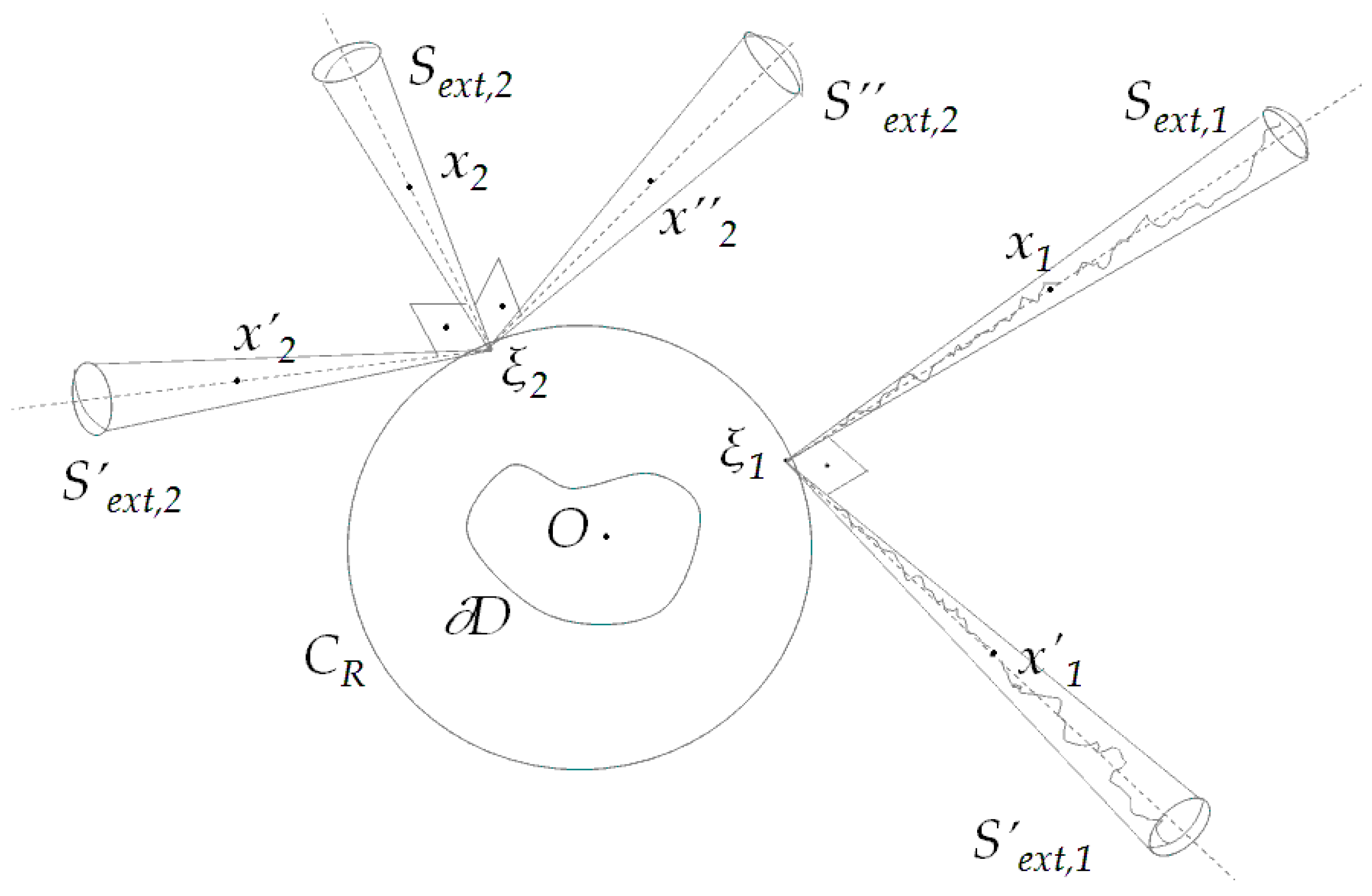
4]. In our case this is accomplished only if we insert into the conical structures interior protective surfaces, thus avoiding the sets on which the driving terms become irregular. In
Figure 1, we give the generic slightly modified conical region supported by a large cup and a small spherical shell deteriorating the singular point
as well as a specification of this region by selecting the protective interior conical surface to coincide with
. The regions under discussion are defined as follows:
and
(with small positive parameters
). The first case is the most general selection while the second one is going to be the most profitable for the application of the methodology.
3.1. The Probabilistic Analysis of the Stochastic Differential Equations Related to the Scattering Problem
Applying Equation (
13) with
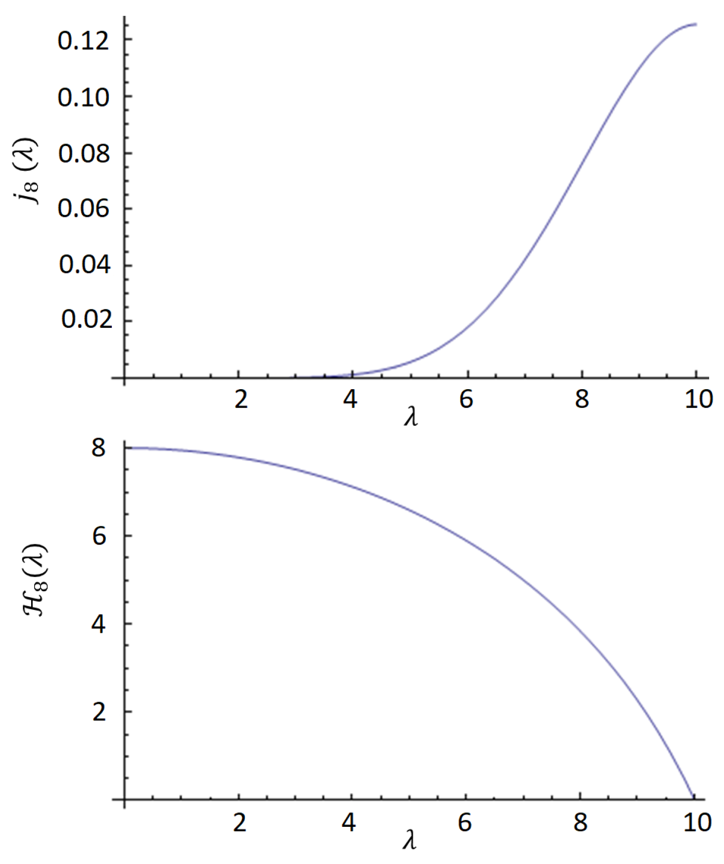
and exploiting the recurrence relation of spherical Bessel functions, we find that
with
This function takes the value
m at
, as a simple asymptotic analysis reveals. In addition, it decreases until the first root, while positivity above a lower bound level
is guaranteed when
, where the values
are uniquely determined due the monotonicity of
(see
Figure 2). It is noticeable that the sequence
increases (
), while their specific values are very useful in the numerical treatment of the problem, as will be clarified in forthcoming sections.
The parameter L, defining the height of the detached exterior space , is usually selected equal to the value .
The following result concerns the duration of the stochastic process traveling inside .
Proposition 1. Let the starting point x belong to . Then the expectation of the first exit time τ (from the detached exterior space ) is estimated as follows: Proof. We apply the It
formula (see [
4]) to the function
and obtain in tensor form
We find that
and
, where
I is the
identity tensor. Consequently, Equation (
19) becomes
The products
and
must be determined via the stochastic differential Equation (
15) and the usual infinitesimal product relations of It
calculus. Indeed, we obtain
Integrating, taking the expectation value and exploiting the independence of
,
, we obtain
Given that
we obtain Relation (
17). On the basis of the restriction
, Relation (
17) easily provides (
18). □
One immediate consequence of the above result is that . So, as expected on the basis of the repellent role of the auxiliary point , the paths are mostly forced to move outwards.
One important issue concerns the probability of the trajectories approaching the lateral surface. We recall that the interior conical protective surface serving at avoiding singular behavior of the driving term is no longer impenetrable, although it retains a repelling role.
Proposition 2. If the domain of the stochastic process (15) is and τ is the first exit time from this domain, then the probability of escaping from the lateral surface, instead of the cups, converges to zero as the parameter ϵ tends to zero: Proof. We apply the It
formula to the function
(
), where
satisfies the Helmholtz equation, and obtain straightforwardly that
Equation (
24) will be repeatedly exploited in the sequel. In the meanwhile, we select
, obtaining
where the independence of
is again exploited. Let
denote the subset of the
-algebra
representing the status of escaping from the lateral surface via points satisfying
. More clearly, we set
Then the set appearing in the statement of the current proposition represents the subset of supporting escaping from the lateral surface independently of the distance from the auxiliary point ; it is identified clearly with the set , simply denoted by .
Similarly, it holds that
. The argument in expectation term of Equation (
25) is positive and so by restriction over specific probability subsets, Expression (
25) gives
Applying Jensen’s inequality for conditional expectations [
14] to the convex function
, we find that
Given that
, Equation (
28) becomes
On the basis of Relation (
18), the direct estimate
helps in modifying Equation (
29) as follows
where
is a well known increasing function with zero limiting value as
. Evoking the increasing inverse function
(which also vanishes as its argument goes to zero), we find that
Thanks to
and the aforementioned properties of
, it holds that
□
The Estimates (
30) and (
31) are rigorous and ensure the convergence regime established in the above proposition but their intrinsic form is not directly exploitable when a rate of convergence is explored. To facilitate the analysis, we introduce a time threshold
T and investigate its influence in cases where we consider the stochastic process with a life time less than
T. In practice, the numerical experiments revealed that the driving term is strong enough to force a short finite time travel inside
. Paying attention to this situation we state and prove the next proposition.
Proposition 3. If the domain of the stochastic process (15) is and τ is the first exit time from this domain, then the probability of escaping from the lateral surface, instead of the cups, in finite time T has the estimate Proof. Equation (
25) gives that
which coincides with the second result of the proposition. Equation (
33) is a direct consequence of the result (
34) if the selection
is adopted. □
The estimate (
33) is useful only when the modification of the original cone is very small. Actually, the term
is always greater than unity and so only when
is appropriately small does this probability estimate acquires a fruitful asymptotic content. Moreover, the result (
34) merits its own attention since it assigns the appropriate probability to lateral escapes confined in the region
. In particular, when
the term
becomes significantly less than unity and contributes essentially to the determination of the probability estimate, verifying the small likelihood of trajectories orientated inwards concerning the vertex of the cone.
The next issue is to estimate the probabilities of escaping from the possible exit surfaces in the case of the domain . In fact, it is now possible to give strict values to the probabilities of hitting the spherical cups of the structure .
Proposition 4. Let the height of be selected as and select a small variable . Furthermore, let the surface of the inner spherical cup belong to . Referring to the stochastic process generated from a point x of the axis of the cone and evolving in , it holds thatwhere the angle is slightly smaller than the angle defining the lateral surface of . Proof. We consider the auxiliary function
, where again we use the spherical coordinates of the local coordinate system attached to the cone
. Clearly,
v belongs to
inside
and vanishes on the lateral surface of region
. We apply once again Dynkin’s formula for the field
, obtaining
Denoting
, we find that
Exploiting that
vanishes on the lateral surface, we split the equation above as follows
where the subscripts in expectations denote the two cups of the region
. Working similarly with the auxiliary field
(instead of
v), we infer that
So far we have selected the height of the cone
L equal to
. In fact, the parameter
defines a range of radial distance, inside which the crucial part of the driving term
remains strictly positive. In addition, inside the interval
, the spherical Legendre functions
are permanently opposite and free of zeros. Actually the same situation holds for the pair
of the Bessel functions of order
since as mentioned above the sequence
increases. Substituting then again
and solving the algebraic Systems (
39) and (
40), we find the unique solution
The denominator in these expressions cannot be zero due to the monotonicity properties of the involved functions. In most cases .
We notice that the function
increases in
, taking values from 0 to 1. More precisely, it rapidly increases in the vicinity of
and then approaches unity almost horizontally. These qualitative results concerning the monotonicity of
guarantee that there always exists a threshold
greater but very close (the angle
is slightly less than
) to
, such that
when
and
. These remarks help first in exploiting Equation () as follows
coinciding with Equation (
36). On the other hand, Equation (
41) provides easily
as stated in Equation (
35). □
Remark 1. It is worthwhile to notice that Equation (43) predicts, in most cases, negligible values for the probability of hitting on the interior spherical small cup. Indeed, having in mind that and thus adopting the reasonable simplification , we obtain that In the case that the arguments and belong to the realm of validity of asymptotic formulae for the involved special functions, we find thatwhich avoids being negligible only when the starting point is forced to be located closely above the inner cup. The situation remains unaltered even if the arguments and escape the asymptotic realm as the investigation of special functions imposes. Furthermore, Equation (35) can be easily weakened to offer a simpler (though underestimated) lower bound: When the point x is even slightly detached from the inner cup it holds that . Then the lower bound of the probability obtains the form . It is remarkable that this ratio involves the starting point and the height of the exterior cup alone. It is obvious that , a fact assuring the total accumulation of hitting points on the exterior cup when γ converges to zero.
For completeness reasons, we state the following result.
Proposition 5. Let the assumptions of Proposition 4 be valid except that the initial point x of the process is not located necessarily on the z-axis but potentially forms a polar angle with it. Then the probability of escaping from the lateral surface obeys the rule Proof. Imitating the arguments presented in Proposition 4, we easily see that the detaching of
x from the cone axis has the consequence of changing Formula (
38) as follows:
Proceeding similarly, we find that Equations (
41) and (
42) are replaced by relations
from which we deduce that
□
The closer the angle is laid to the zero value, the more is suppressed to zero, under the validity of the relation , induced by Remark 1. In contrast to that, when approaches , the factor goes to zero, taking down with it the probabilities and and amplifying drastically the appearance of lateral crossings. This is the reason we insist on locating the starting point of the stochastic process on the cone axis and then eventually eliminate the probability of lateral surface hitting.
So far, we have studied some basic qualitative properties of the trajectories representing the solutions of the underlying stochastic differential equations and derived estimations for some crucial probabilities concerning the hitting points of these trajectories on the components of the boundaries. Two cases have preoccupied our interest: The general case
as well as the more special conical region
. It will be clear during the implementation of the method that a result of the type (
31) pertaining to the first case would be useful—actually in a stronger form—even for the second case as well. In this direction, we state and prove the following lemmata.
Proof. The It
formula gives
from where we obtain the sought result via time integration. □
Lemma 2. For every , it holds that Proof. Equation (
24) is equivalent to
Integrating over time until the first exit time and taking the expectation value as usual, we obtain
The argument inside the expectation of the last expression can be handled via the previous lemma as follows
Combining Equations (
49) and (
50), we find that
□
The next proposition extends the main result of Proposition 3 not only for referring to the alternative conical structure but mainly for ameliorating the rate of convergence as diminishes:
Proposition 6. If the domain of the stochastic process (15) is and τ is the first exit time from this domain, then the probability of escaping from the lateral surface, instead of the cups, in finite time T has the estimatefor any real . Proof. Thanks to the monotonicity of the spherical Bessel function, Jensen’s inequality for conditional expectations and the independence of
, Equation (
48) is transformed as follows
Renaming to we have what the proposition states. □
We mention here that we restrict ourselves to the interesting case
. Actually, the result with
is an immediate consequence of Proposition 3 with
sufficiently small so that the right hand side of Equation (
33) is less than unity. The selection of
is related with the total travel time
T. The exponential term remains small when the term
does, where the wave-length
of the process appears. The quantity
commonly emerges in stochastic processes involving appropriately the space and time dimensions.
3.2. On Deriving Stochastic Representations for the Scattered Field
At this point, the involvement of the physical field representing the scattered wave
u presented in
Section 2 takes place. We recall that this field belongs to the kernel of the Helmholtz operator. Our aim is to embed appropriately this field in Dynkin’s calculus, which has already profited throughout the treatment of the stochastic process under consideration. More precisely, considering the field
, we are in a position to apply once more Dynkin’s formula leading to the stochastic representation
Denoting
, we find that
Working in
, the last relation obtains the form
where we have taken into account the less probable but still possible event of stochastic escaping via the lateral surface of
.
The Representation (
55) constitutes one of the fundamental results of this work and will be a subject of investigation during the examination of the inverse scattering problem. It has a local character since it is valid in a conical region
surrounding point
x and defines a specific portion of the exterior space. It constitutes a stochastic representation of the value of physical field in the point
x, involving three terms corresponding to stochastically first time escaping events from the two spherical cups and the lateral surface of the cone. The severe or mild implication of every portion of the manifolds, where escaping takes place, has been revealed previously in this section. In brief terms, the Representation (
55) favors the information offered in the exterior cup at the same time that it suppresses the importance of information that has taken place on the inner cup and eventually eliminates the involvement of the lateral surface. So this representation seems to be more adequate when we are interested in deriving a continuation of the remote field to the near field.
The immediate question arising on the basis of this discussion is whether there exists another stochastic representation giving priority to information on the interior cup and suppressing the involvement of data on the exterior spherical shell. This representation would have the character of a near to remote field transformation. This is actually accomplished by giving a primitive role to the auxiliary function
instead of
, which has been exploited so far. Taking advantage of the recurrence relation of spherical Bessel functions, we can transform Equation (
13) in the following form
with
This radial driving term is now negative (
Figure 3) and has opposite behavior compared to
. It is not the goal of this work to repeat all the theoretical investigation for this new stochastic differential System (
56) but it is now recognizable to follow the main characteristics of the stochastic trajectories ruled by the negative driving term (
57).
We remark easily, imitating the arguments presented in Proposition 1, that
and so we expect an inward directivity of the new set of trajectories. Actually, in the new situation, the point
is not a repellent point but an attractor for the stochastic paths. Indeed, a straightforward application once again of the concepts presented in Proposition 4 leads to the estimations
with
As special function properties reveal, is, for most of the parameter cases, close to unity, while lies in the vicinity of zero. Actually, we meet here the mirror situation, in which the trajectories starting from the axial point x converge inwards, attracted by the vertex .
Working in
, we are in a position to present, in a way analogous with Equation (
55), the representation of the scattered field in terms of the inward directed stochastic process:
The fundamental Expressions (
55) and (
59) give the essential basis to design the geometric characteristics of the conical structure. A common feature in these expressions is the presence of the ratios of spherical Bessel functions defined on the point
x as well as on the external and internal surface of the cone. These fractions can obtain very unbalanced values in the case that the position arguments are chosen arbitrarily. This is expected since these coefficients multiply expectation values of different orders due to the imposed conditional stochastic laws. So the selection of the geometrical characteristics of the detached conical region should obey the necessity to allow high sensitivity on revealing all types of data. In addition, the third terms in both representations incorporate a ratio between two controversial terms: The expectation value over the very few lateral escaping points and the very small value of the Legendre term
. This is a very interesting tag of war, whose investigation has caused the probabilistic analysis leading to Proposition 6. Actually, apart from the possibly large period of time
T, the mentioned ratio is proportional to
,
, which converges to 0 as
. These and relevant matters merit special treatment when application of the method takes place in the next section.
The Representations (
55) and (
59) have been built on the basis of, respectively, strongly outward and inward moving stochastic trajectories. They develop by nature a strong preference to represent the field at
x by data confined in the far field domain or the near field region, respectively. What remains is to explore the possibility of constructing a representation giving an equivalent role to the spherical cups and still deteriorating the role of the lateral surface. This can be realized via the implication of a modified driving term that stemmed from a linear combination of the spherical Bessel functions
and
. In fact, we start with the modified auxiliary function
, where the mixture coefficient will be determined methodologically later on. This radial function gives birth to the Helmholtz equation solution
, which as usual generates the set of stochastic differential equations
where
The stochastic representation obtains now the form
To reveal the special features of this representation, we need to explain its particular building. The selection of the parameters has a hierarchical structure. The cone
defines the crucial dimensions
and
. Then the coefficient
in the definition formula of
is chosen such that the function
obtains the same values at the end points of its domain, i.e.,
. This means that
Then the coefficients
and
of the first two terms of the Representation (
62) are equal and the equipartition has arisen as a possibility. What remains is to ascertain that the probabilities of hitting the two cups are comparable. This can be realized if the point
x is appropriately selected. To show the selection criterion for the observation point, let us examine the example pictured in
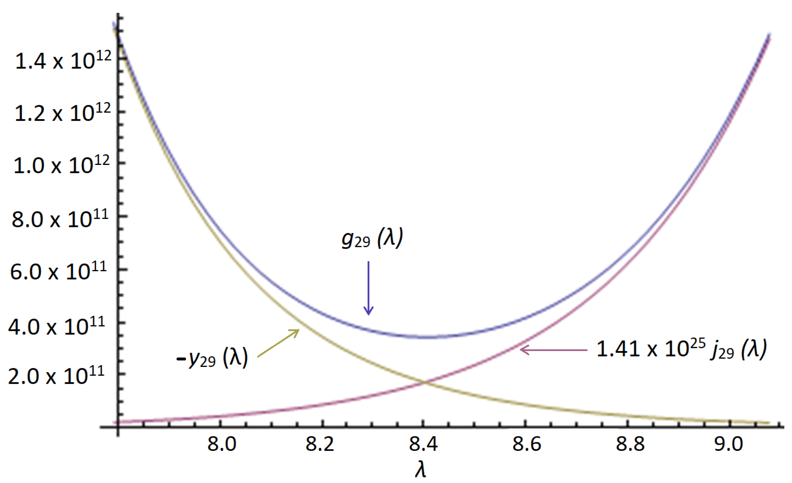
Figure 4.
We remark that the modified driving term
is separated into two branches—each one coinciding with one of the driving terms of the older stochastic processes—plus an abrupt transition region from the one situation to the other. The function
vanishes when
becomes zero, as implied by Equation (
61). The imposed condition
and the specific monotonicity behavior of
in the interval
guarantee the existence of only one point
where
vanishes and simultaneously
takes its minimal value.
As a simple analysis reveals and
Figure 5 demonstrates, the constituents
and
of
take the same value near the minimum point
, i.e.,
The unique point
x, satisfying Equation (
64), is selected to define the initial point
x of the stochastic process. Every trajectory emanating from
x is subjected, in the beginning of its travel, to a pure Brownian boost since the driving term is locally zero. So its initial directivity obeys the Brownian law, but once it finds an orientation, the driving term obtains abruptly one of the already studied inward or outward behaviors, pushing the trajectory to cross the corresponding cup. Intuitively, one half of the trajectories meets the exterior cup, while the other half escapes from the smaller inner spherical shell. This indication can be verified rigorously. Indeed, the above encountered probabilistic analysis applies again to define estimates of the hitting probabilities. Following the argumentation met in Proposition 4, using Equation (
64) and the asymptotic analysis of the involved special functions, we find that
The design of the geometrical parameters involved in the third representation has been applied in a specific sequence, which will be proved useful in the framework of the inverse problem. As far as the direct problem is concerned, the reasonable hierarchy is a little bit different: The first concern is the selection of the observation point
x and the next step is the determination of the coefficient
appearing in
by demanding the validity of relation
(see Equation (
64)). Then what remains is the determination of the interior and exterior radii
. These parameters could be selected arbitrarily but in that case the probabilities of escaping through the shells would be of different order and then the coefficients
and
of Representation (
62) would be unbalanced in order to compensate this unfitness. If equipartition of escaping is desired then the one parameter is selected freely and the other one must chosen (the selection is unique) so that
. Additional criteria concerning the choice of the free parameters have numerical origin and will be presented in the next section.
Summarizing, the Representation (
62) gives an equivalent role to the exterior and interior spherical shells since the involved coefficients are balanced to keep the same order while the probabilistic status favors the equipartition of the produced trajectories. The third lateral term is again predominated by the term
,
and fades away when
. The Representation (
62) is the conditionally probabilistic analogue of Green’s integral representation in the direct scattering problem with the advantage of validity on cropped conical portions of the exterior space having as spherical cups subsets of the far field region and the scatterer’s surface.
4. The Application Features of the Stochastic Implementation
The stochastic differential Equations (
15) can be slightly modified on the basis of recurrent relations valid for spherical Bessel and Legendre functions, thus providing the discretized Euler scheme [
15]
Similarly, the dual stochastic differential System (
56) leads to the discretized scheme
Both Euler schemes (in [
7], we presented an approach of higher accuracy leading to a stronger Taylor scheme inspired by [
15], but this is not necessary in the framework developed herein) are sufficient in the case of relatively spacious cones and their comparison with the static case [
7] reveals the influence of the wave number
k. Examining first the Scheme (
68), we see that when
, we take the stochastic framework encountered in [
7]. Consequently, in the absence of
k, the term
has the main contribution to radial driving of the stochastic process, representing mainly the attraction of the conical vertex
.
However, the situation changes drastically when handling the stochastic law (
67). This can be easily conceived when
and the asymptotic regime for the spherical Bessel functions is evoked. Then the term
tends to zero and the dominating factor in drift is
, forcing the trajectory to move upwards, as already predicted analytically in previous paragraphs. In addition, the terms
do not allow the paths to move far away from the local
z-axis.
The combined Scheme (
60) merits its own attention, but, as already explained, the initial direction of the trajectory activates one of the possible branches (the outward or inward scheme) that have been described above. Actually, every numerical experiment is evolved with probability one half via the rule (
67) or (
68) exclusively, since going back in the opposite direction has a tremendously small likelihood.
Having in mind the remarks above, we focus on the first stochastic System (
67) and investigate the geometric ingredients of the conical region
where the Representation (
55) applies. As far as the crucial parameter
, defining the height of the cone, is concerned, it is necessary that
is slightly less than the first local maximum point of
. To clarify this criterion, we present for example the case (
) in
Figure 6.
It is clear that only when
is chosen to be less than the first maximum point
of
, the driving term
remains positive in the whole interval
. To take advantage of all the available space, it is preferable to choose the parameter
to be less and close to the first maximum point
of
. In
Table 1 we see some important cases which will emerge in the applications. It is noticed that the appeared height of the cones is the maximal possible for every particular
m. Nevertheless, we have the flexibility to select smaller heights if this is useful.
When
m augments then the parameter
(the height of the cone) increases while the cone becomes narrower as the interior protective cone is defined by the angle
, which is a decreasing sequence. The selection of the parameter
is based on the remark that in the beginning of the process, the driving term offers an axial boost
, which becomes extremely large when
x approaches
. Then if we are interesting in assigning rapid directivity to the outward orientation of the process, we are obliged to design a small distance
, a fact rendering even smaller the distance
. In most of the numerical experiments of the outwards orientated stochastic cluster, the reference selection
was adopted in connection with the choice
. What remains is defining the parameter
for every particular
m. Referring to Equation (
55), the second term
has a coefficient of order one thanks to the proximity of the arguments
and so this term is governed by the very small probability of first exit from the interior shell, being so suppressed. The first term
is strongly favored by the probabilistic law since the majority of the trajectories hit this cup. This term has apparently a generally small coefficient
—due to the monotonicity of the Bessel function—but this just implies that the main contribution of the expectation is produced from strikes near the angle
where the denominator takes small values. It is important to determine
in a normalization sense in order for the leading term of the representation to be implemented numerically efficiently. There are several good choices, as numerical experiments revealed, but the optimized one has an exponential structure. One convenient choice leading to a balanced representation, as will be verified later, consists in taking
such that
where we meet the parameter
introduced in Proposition 6. This is always possible since
monotonically as
goes to zero. Then, the first leading term of Representation (
55) is an expectation involving the field
—over the exterior cup—with a multiplicative function
, which (as we move to the circular boundary of the cup) approaches the value
that equals
, which is greater (it holds that
, when
) than
. Consequently, the greater the parameter
, the stronger the weighting of the involvement of the marginal hitting points near the peripheral circle of the exterior cup. This has a parallel pace with the diminishing of the estimate expressing the contribution of the whole lateral conical surface. Indeed, evoking Proposition 6 (applied with
), the lateral term is bounded as follows:
The discussion above offers some a priori analytical origin to the selection criteria of the several involved parameters, whose final choice obeys of course the specific characteristics of the separate particular cases encountered in next sections.
5. On Exploiting the Remote Field via Stochastic Analysis in the Service of the Inverse Scattering Problem
In this section it will be demonstrated how the far field information is transferred on the surface of a sphere enclosing the space that is occupied by the scatterer and belonging to the regime of the near field. This sphere is centered at the coordinate origin O, has radius R and could be the circumscribing sphere of the scatterer. If the scatterer is a convex structure then the sphere could be replaced by the surface of the scatterer itself and this is a special and interesting case that merits separate treatment and is presented in the forthcoming subsection.
The goal is to transfer the data given in the far field region on the surface of the sphere
. What is offered as data is the far field pattern or equivalently the Dirichlet to Neumann operator (for some possible selections of the directivity
of the incident wave) in a large sphere with radius
equal to a few wavelengths. Focusing on a specific orientation
, the distance
has to be interpreted as the height
L of a cone
, having as axis this orientation and as vertex the uniquely determined point
of the sphere
(see
Figure 7).
This selection gives birth to the dimensionless quantity
, which must be fitted with the appropriate parameter
discussed earlier. In other words, we have to select the appropriate order
m such that
is slightly smaller than the first maximum point of
. The interior cup of the cone is selected via the choice of the parameter
, which as discussed in the previous section is assigned a considerably small value for several reasons. Then we construct the appropriate combination
, by selecting
via the rule (
63), assuring that
obtains the same values at the upper and lower cups of the cone (
). Given the parameter
m, the angle of the cone is defined uniquely and equals
. Then the starting point
of the stochastic process is selected according to the Formula (
64). We recall that this choice establishes the equipartition of spreading of trajectories towards the cups of the conical structure. We proceed then to the solution of the stochastic differential System (
60) in combination with Equation (
61) and the starting condition
. As discussed above, every numerical experiment obeying to the aforementioned stochastic law, splits with probability
to one of the dual numerical Schemes (
67) and (
68) presented in
Section 4. The crucial point though is that Formula (
62) is adequate to apply not to the physical field
u but to the vector field
. First, this is legitimate since the field
M belongs to the kernel of the Helmholtz operator. It is actually reminiscent of one of the three respectively perpendicular Navier eigenvectors constructed on the basis of a scalar solution of the Helmholtz equation, via repeated suitable application of the curl operator. Secondly, it is an efficient choice since
M constitutes a null field at the point
. This annihilation leaves active in the stochastic representation only the contributions of the field on the spherical walls of the conical structure. On the basis of the equipartition property
and Relation (
70), the Equation (
62) becomes
For large
(which affects slightly but effectively
and the cone via its angle) the right hand side of the last equation fades away exponentially. In addition, given that
, the interior cup is shrunk and the expectation value over it behaves as
, where
. So we obtain what is a simple but one of the fundamental results of this work:
expressing the tangential derivative
over the the sphere
at the point
. Then knowing
(this is not identical to the information offered by the far field pattern but strongly related to that. It is of course reminiscent of the gathered information offered by the Dirichlet to Neumann operator for a specific wave number and a concrete direction of incidence. See Remark 2) on the suitable portion of the far field region leads to the determination of the tangential derivative of the field on the—potentially–circumscribing sphere of the scatterer. If we are interested in determining fully the gradient of
u in
, we need to repeat the process above via the implication of a cone
with the same vertex
, vertical axis normal to the axis of
and identical geometrical parameters. This process incorporates a new set of numerical stochastic experiments concerning now the stochastic process
involves data on a different portion of the remote region (see
Figure 7) and provides that
where
is normal to
and
. Determining thus
and
implies reconstruction of the full vector field
. The last assertion holds even in the case that the surrounding surface is not spherical and so the vector
is not necessarily the normal vector on the surface. The same situation can be repeated for every arbitrary point
located on
. The selection of the secondary perpendicular cone is arbitrary and depends on the availability of data (see
Figure 7).
Combining Equations (
72) and (
73), suppressing indices, setting
and exploiting the identical geometric characteristics of the cones, we easily prove that
In fact, it is not always necessary to use a different set of cones (and far field subregions) for every particular point
of the surrounding near field surface. This remark can be explained in a converse manner introducing the well known case of the restricted far field data. The question is to determine the range of influence of this restricted set. Indeed, let us assume that the vector
is measured on a portion
of the remote field regime. As depicted in
Figure 8, the surface element
defines a truncated cone
which divides the surface
into two parts, the shadowed one and its complement
, on which a grid of points
can be distributed.
Every such point constitutes the vertex of a cone whose base is the sub-surface
. These cones do not have—in their majority—upper spherical cups orientated with their axis
, but this geometrical slight declination does not affect the probabilistic setting developed so far given that the influence of the bases to the evolution of the trajectories applies only to the final steps of their travel. In summary, if only
are to be determined (for a plethora of points
,
on
), then the information on
is enough. Moreover, if we are interested in determining the vectors
themselves, we evoke the dual perpendicular cones (as demonstrated in
Figure 7) whose base assembly forms a supplementary far field data region of indispensable utility.
The method will be accomplished after the determination of
u itself on
is fulfilled. We consider the—perpendicular to
M—vector solution of the Helmholtz equation
. It is easily proved that the scalar field
belongs also to the kernel of the Helmholtz operator and is annihilated clearly at the point
. Let us, for example, pay attention to the stochastic Representation (
62) in connection with the conical structures with vertex point
of
Figure 7. We take into account three mutually vertical cones
(geometrically identical) and apply Equation (
62) to the Helmholtz equation solutions
and
, respectively. We obtain then
In the far field regime and especially on the three surface portions , the field has the asymptotic behavior , where we meet the well known Beltrami operator . In Remark 2, we investigate the characteristics of the function and its mining mechanism from the offered data.
We proceed by adding the Relations (
75) for
. The left hand side of the produced equation is proved to be equal to
, if we take into account that
u satisfies the Helmholtz equation. Taking the interior expectations to be identical and suppressing subscripts (referring to a generic point
), we obtain
Exploiting Equation (
74), we find
which constitutes one of the basic results of this work.
Remark 2. The scattered field , obeys the Atkinson–Wilcox expansion [11]outside the circumscribing sphere (), where we encounter the radiation pattern , which appeared in Equation (4). In second order approximation, we have the following asymptotic form for the remote field: The coefficients are related via the well known [11] recursion scheme , . So the field that appeared in the Representation (76) is expressed asinvolving thus the second order approximation of the remote field expansion. The direct detection of in measurements via (78) is complicated and demanding since it requires high sensitivity analysis and suffers from the implication of measurement errors. However, its determination via a posteriori analysis of data is straightforward: The far field pattern always has expansion in terms of the spherical harmonics (Ω
stands for the unit sphere). Theoretically, in the absence of noise, the coefficients rapidly decay, satisfying [16] the growth condition . In practice, the coefficients are calculated via the integrals that appeared in (80) on the basis of the measured far field and then an expansion of the possibly polluted pattern in terms of spherical harmonics (see again (80)) can be constructed. Due to noise, the expansion coefficients of could violate the aforementioned growth condition but generally maintain a rapidly decreasing behavior. Thus, the field is represented as the expansion , taking into consideration the fact that the spherical harmonics are the eigenfunctions of the Beltrami operator (). The last expansion represents a stable estimation of in the case that the noise corruption does not alter the before-mentioned growth behavior to such an extent that the reasonable and much weaker summability condition is violated.
The same process is followed to construct numerical implementations of the remote vector wave field , participating in the expectations that appeared in representations (74) and (76). Indeed, in the case that the starting point x of the stochastic process is designed to belong to the near field region and especially close to the vertex ξ, the function behaves like as , where we recognize the spherical surface tangential gradient . Evoking the spherical harmonic expansion of the far field pattern, we find thatwhere there emerges, for every pair , one of the Hansen mutually orthogonal vector spherical harmonics (i.e., the eigenvectors , and ). The final step of the method is to implement the Representations (
74) and(
76) by evoking Monte Carlo simulations of the emerged expectation values over the spherical cups. Thus, for every cone under consideration we perform
N repetitions of independent stochastic experiments, providing trajectories obeying the stochastic differential System (
60). These trajectories are gathered and special attention is paid to their traces over the exterior and interior surfaces of the cones. On these exit points, we calculate the contribution of the involved fields, which are present in the expectation arguments and take appropriately the mean values of the accumulated terms. Consequently, Representation (
76) acquires the numerical implementation
where
represents the number of exits of the trajectories through the exterior surface of the cone
. Given that the involved cones in Representation (
76) are identical, then
. In addition, the theoretically established equipartition of the trajectories, pertaining to their orientation, implies that
, a fact which is approved by the experiments.
On Reconstructing Convex Scatterers
We consider in this section the pilot case of convex scatterers. As discussed above, the developed analysis of transferring data from the remote region to the near field region can take place up to the surface of the scatterer given that it is feasible to exploit a system of cones which do not intersect portions of the scattering bodies. Then, the surface
is an assembly of all the points
,
on which the right hand side of Equation (
76) equals
, satisfying thus the boundary condition (
2). The motif is to reveal that only one direction of excitation is sufficient to provide adequate inversions, and so the case
will be examined uniformly for all the case studies.
In the beginning, we consider the primitive case of a spherical scatterer of radius
a, centered at the coordinate origin. Being more specific, we consider the simple case of
and
. The needed synthetic data are produced via the well known representations [
16] of the scattering field and the far field pattern:
So, the terms
, representing the spherical harmonic expansion coefficients of the far field pattern are equal to
and play an important role to the construction of the arguments of the forthcoming numerically simulated expectation terms involved in the functions
,
, denoting the right hand side of Equation (
76) for several points
, sampled uniformly inside a cube
centered at the coordinate origin and having edges of length
. This cube hosts the determinable scatterer. We consider a remote distance
of order of
where the synthetic data are collected. We focus on the portion of data that is confined on a spherical subregion of the sphere
around the radial direction
. The aforementioned choices define the crucial geometric parameter
, defining the range of the remote scattering field and the typical size of the involved cones. So, according to the parametric analysis described in previous sections, the integer
m takes the optimal value
. The abovementioned range of used data
(on the sphere
and in the vicinity of
) has a spherical polar aperture confined by the angle
. (We recall that the supplementary data introduced by the dual perpendicular cones of type
and
play also a crucial role). The vertex of every involved cone
is one of the sampling points
; its interior cup is very close to the vertex via the selection
, which leads to a concrete Helmholtz kernel
so that the equilibrium
is established. This description defines the typical geometrical characteristics of the involved cones so that the interrelation between the remote and near field region is exploitable. Using again the parametric analysis exposed previously, the starting point
of every individual stochastic process taking place inside
should belong to the axis of the cone and distances from the vertex of a specific length so that the equipartition of the directivity of the trajectories is ensured (see Relation (
64)). Then, the geometrical feature
for the involved cones, is determined to have the exact value
. The hitting probabilities are theoretically foreseen by Equations (
65) and (
66) to be
and
and the simulations verified this prediction.
Prescribing further the performed numerical experiments, it is noticed that inside the cube
, a set of
uniformly distributed potentially candidate surface points
has been sampled and for every
, stochastic experiments have been performed pertaining to the solution of the underlying stochastic differential equations in the cones
,
and
. If additional a priori information was given about the possible location of the interface
, the distribution of the sampling points
would have selective characteristics. In any case, the Monte Carlo realization of the involved expectation terms required at most
experiments—repetitions with a typical life time of traveling inside the cones expressed via the rule
. This result is in conjunction with the uniform selection of the parameters
and
, defining in detail the angle of the cones according to the results of
Section 4. This stochastic implementation led to the determination of the stochastic terms
,
, expressing, as mentioned before, the right hand side of Expression (
76).
The inversion algorithm consists in constructing and investigating the objective function
. The points
assigning small values to the functional
are the supporting points of the surface
. In
Figure 9, we plot the level set of the interpolating function
, representing the set of points satisfying the criterion
with
.
We verify the high level of accuracy in the reconstruction as far as the region of influence of
is concerned (
Figure 8). It is reasonable that the points
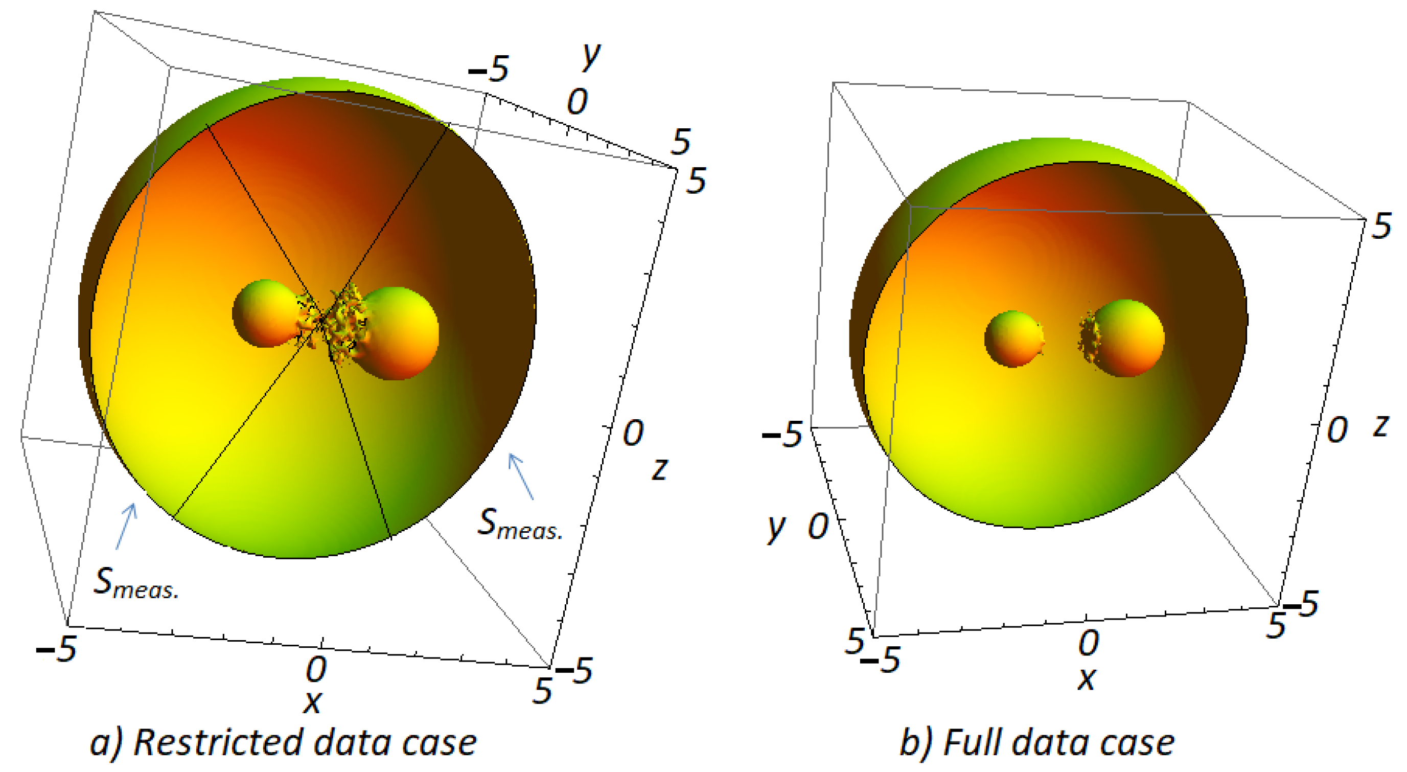
belonging to the shadowed region cannot be reconstructed appropriately, since they pertain to cones intersecting the scatterer and occupying regions, part of which do not belong to the real scattering region. Actually this is the drawback when non-convex scatterers are investigated since the stochastic representation has been formulated on the assumption that the trajectories are free to move in subregions where the underlying Helmholtz differential equation is valid. (In this case, we reach similarly the circumscribing sphere and proceed further differently as will be clarified in the next section)
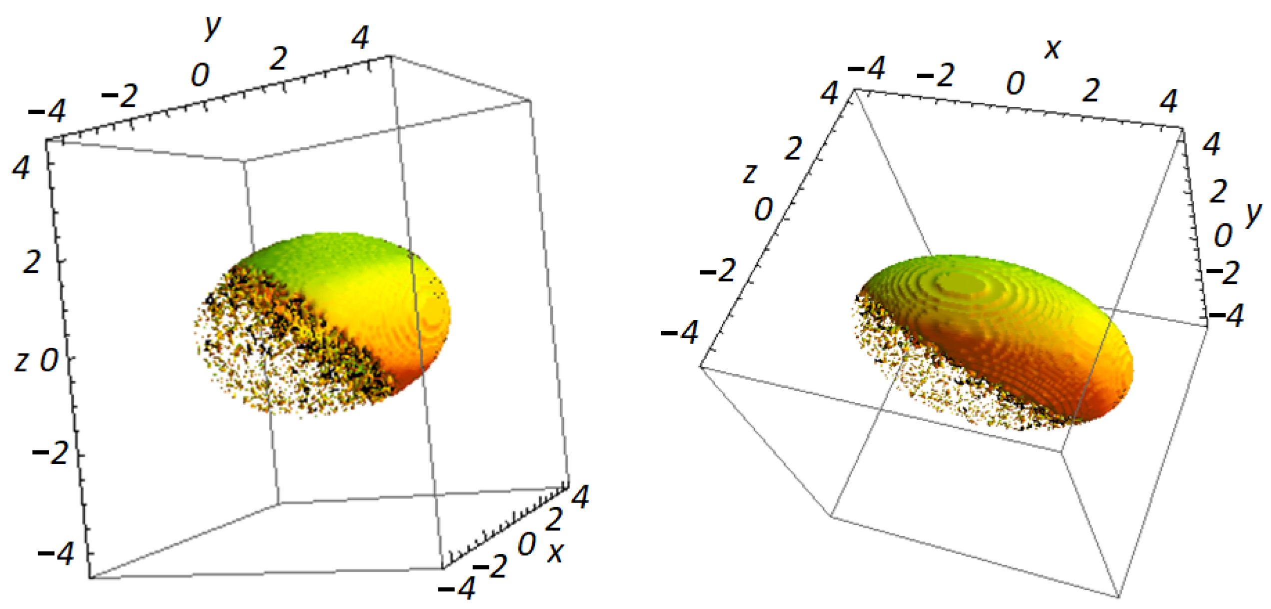
The presented methodology has been applied also in the case of the inverse acoustic problem by the ellipsoidal surface
with considerably unequal semi-axes
. In order to avoid the complexity of the ellipsoidal harmonics [
17] and to open up the rich and simple arsenal of data of the direct problem in the realm of the low-frequency region, we consider the indicative case
and evoke the stable results encountered in [
18] and the developed methodology in [
19]. More precisely, the far field pattern acquires the form
where the well known [
18] elliptic integrals
and
,
are involved.
Insisting on the back scattering setting
, we use (
83) to furnish the necessary data appeared in the mean-value terms of Formula (
82) exactly as we did in the spherical case. The 3D contour plot of the objective function
with
gives the very accurate reconstruction depicted in
Figure 10. The only difference in the parametric setting is that we have adopted a denser grid of sampling points (
) to reveal the strong anisotropy of the scatterer.


