The Instability and Response Studies of a Top-Tensioned Riser under Parametric Excitations Using the Differential Quadrature Method

Abstract

The differential quadrature method (DQM) is a numerical technique widely applied in structure mechanics problems. In this work, a top-tensioned riser conveying fluid is considered. The governing equation of this riser under parametric excitations is deduced. Through Galerkin’s method, the partial differential governing equation with respect to time t and vertical coordinate z is reduced into a 1D differential equation with respect only to time. Moreover, the DQM is applied to discretize the governing equation to give solution schemes for the risers’ parametric vibration problem. Furthermore, the instability region of Mathieu equation is studied by both the DQM and the Floquet theory to verify the effectiveness of the DQM, and the solutions of both methods show good consistency. After that, the influences of some factors such as damping coefficient, internal flow velocity, and wet-weight coefficient on the parametric instability of a top-tensioned riser are discussed through investigating the instability regions solved by the DQM solution scheme. Hence, conclusions are obtained that the increase of damping coefficient will save the riser from parametric resonance while increasing internal flow velocity, or the wet-weight coefficient will deteriorate the parametric instability of the riser. Finally, the time-domain responses of several specific cases in both stable region and unstable region are presented.

1. Introduction

The risers are pipelines linking the seabed and the platform above the sea. Because of the vertically dynamic excitations induced by the heave motion of the platform, the parametrical resonance of the risers would occur, and fatigue damage will follow. To avoid such risk, it poses an urgent demand to make a parametric instability prediction plan at the designing phase of the risers.

The study of the dynamic properties of pipes dates back to the 1970s. From 1970 to 1972, Chen [1,2,3,4] presented a comprehensive investigation of the free vibration, forced vibration, and stability of pipes conveying fluids. Since then, the vibrations of pipes have been drawing attention from researchers. In 1975, Hsu [5] figured out, for the first time in the engineering application, the parametric instability characters of the straight and vertical configuration of a hanging. He analyzed the parametric instability of hanging string risers with a Ω–Γ instability chart and studied the influences of nonlinear fluid dynamic damping on the steady-state responses of risers under parametrically unstable conditions. Later, a lot of classic contributions [6,7,8,9,10,11,12] were carried out about the parametric vibration of risers. Recently, Lou et al. [13] studied the horizontal parametric vibration of a compliant vertical access riser, and mode coupling and damping’s effects on risers’ parametric instability were discussed. Zhang et al. [14] investigates the vibration of a top tensioned riser under both parametrical and vortex-induced excitations by numerical simulation and experiment, and the aggravation of the riser’s VIV response affected by parametric excitation has been evaluated. Liang and Lou [15] studied the effects of multiphase internal flows that consider hydrate phase transitions on the parametric stability of marine risers.

In the current study, a top-tensioned riser subjected to parametrical excitation is studied. For the dynamic problems in engineering applications, some numerical methods, such as the finite element method [8,16,17,18,19,20], Runge–Kutta (R–K) method [7,10], and finite differences method [9], have been verified to be valid and accurate in coping with such problems. Ni et al. [21,22] considered the dynamic problems of a pipe conveying fluid by the differential quadrature method (DQM) and generalized differential quadrature rule (GDQR). They found that DQM and GDQR show good competency in such problems. Illuminated by their works, we decide to consider the parametric instability of the top-tensioned riser with DQM. The DQM was first introduced by Bellman and Casti [23] as a new technique to solve the initial-value problems of ordinary and partial differential equations. Based on such work, DQM was extended into various applications such as fluid flow and turbulence, the Hodgkin–Huxley model, structural mechanics and mechanical dynamics, etc. [24,25,26,27,28]. Furthermore, Wu and Liu [29,30] complement the DQM by introducing the generalized differential quadrature rules (GDQR) to equip this method with the ability to treat high-order differential equations and complex boundary conditions more flexibly. In recent years, the study on DQM continues. Essam et al. [31] proposed a new hybrid linearization-differential quadrature method (HLDQM), and some numerical experiments on a Fe3O4 ferrofluid flow over a vertical radiate plated were conducted by this method. Constantin et al. [32] applied the least-squares differential quadrature method (LSDQM) to nonlinear partial differential equations, and solutions with better accuracy were acquired compared to other well-known methods: homotopy perturbation method (HPM) and the Adomian decomposition method (ADM). Additionally, some novel modifications on DQM have been made to accommodate more flexible situations [33,34,35,36].

Based on the aforementioned studies of the risers’ parametric vibration and DQM, in the current study, the DQM would be introduced to calculate the vibration properties of risers under parametric excitation. Additionally, the effects of some key factors such as damping, internal flow velocity, and unit wet weight on the risers’ parametric instability would be discussed in detail. In Section 2, the governing equation of the parametric vibration of a top-tensioned riser with internal flows and the implementation of solving this governing by DQM was presented, and the deduction of the unstable zone of the Mathieu equation is conducted. In Section 3, the validation of DQM in analyzing risers’ parametric instability is verified with the Mathieu equation; also, the instability charts of a top-tensioned riser under different conditions are given to discuss the influences of different parameters on risers’ instability. In Section 4, the parametrically excited responses of this riser are given. In Section 5, the conclusions are made.

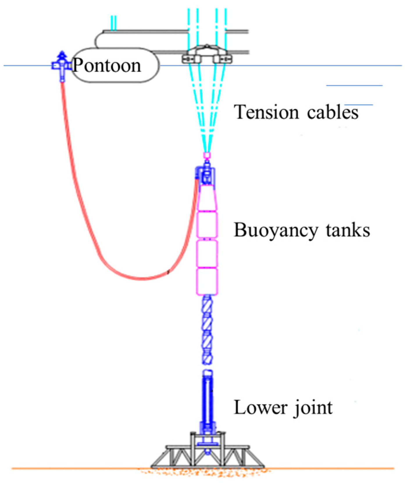
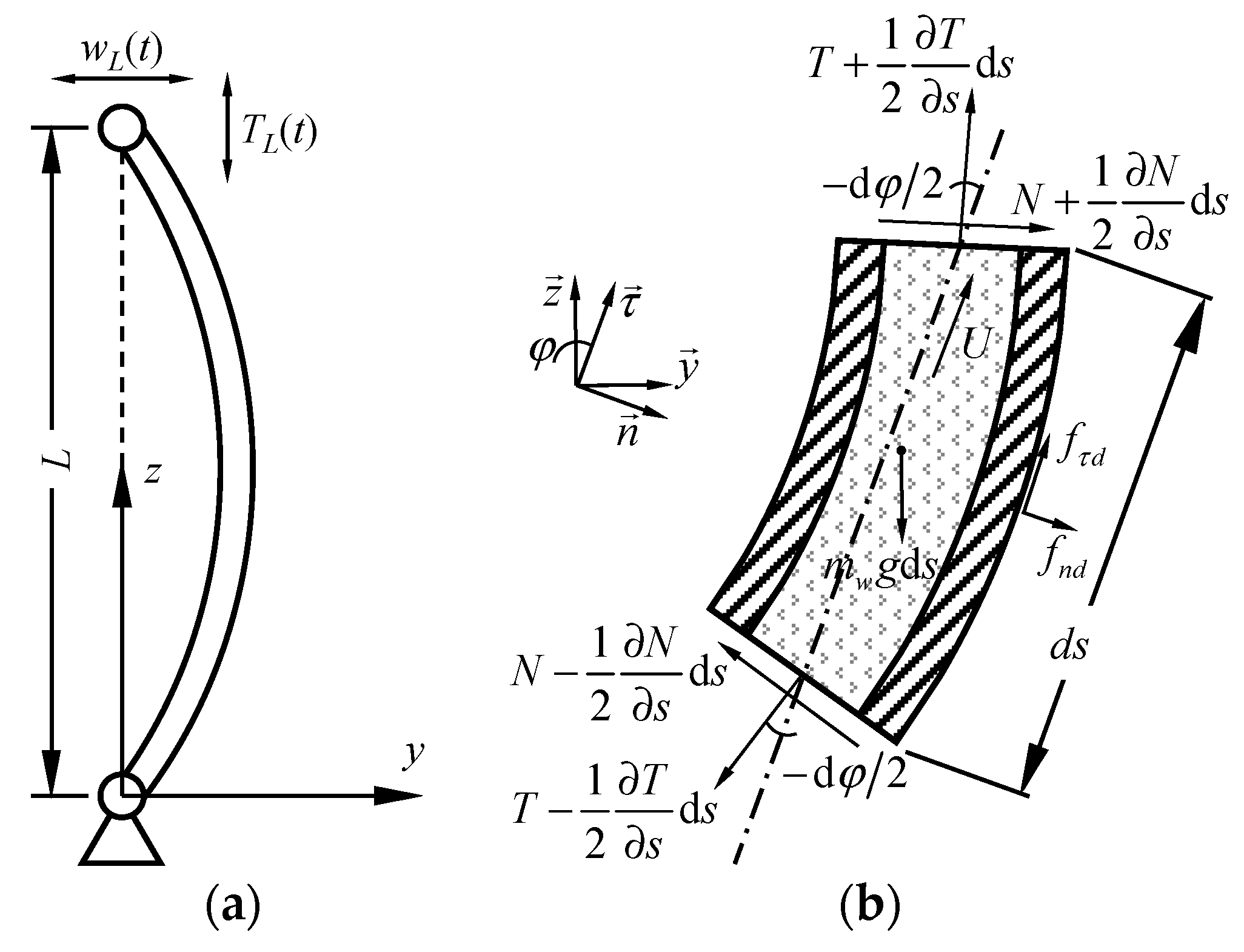
2. Modelling and Method

2.1. Governing Equation of Parametric Vibration

In the ocean oil drilling industry, the riser is an indispensable structure transporting oil from the seabed to the platform. Our study is based on a top-tensioned one whose figure is illustrated in Figure 1. As shown in Figure 1, the riser is hinged at the bottom end and the top of the riser is pulled by tension cables. An array of buoyancy tanks is arranged along the riser to counteract the weight of the riser and provide extra tension to keep the riser erect. Since the use of risers is to transport fluid, there is liquid flowing inside risers. When the platform heaves up and down, the riser will suffer axial dynamic tension, which will generate parametric excitation to the riser.

To transform this engineering model into mathematical expression, some hypotheses are introduced, and a simplification of the riser is given. The material, mechanical properties, and the buoyancy distribution are regarded as uniform and continuous along the length of the riser. Thus, the riser considered in our study can be simplified as a vertical Euler beam hinged at both ends with internal fluid flowing inside it and with uniformly-distributed tension along with it. The simplified structure of this and the force diagram of an infinitesimal unit of this riser are depicted in Figure 2.

The riser is simplified into a 2D beam subjecting to the horizontal forcing displacement excitation u_L(t) and the vertical parametric excitation T_L(t) at the top end. For this infinitesimal unit, there is tension T and shear force N at both ends. m_wg is the unit wet weight, and it equals the difference between the total weight of the unit and the buoyancy of the unit, namely,

$$m_{w}g=m_{s}g+m_{f}g-f_b$$

(1)

where f_b is the buoyancy provided by the riser and the buoyancy tanks of unit length, and m_s and m_f are, respectively, pipe weight and internal fluid weight of unit length:

$$m_s={\rho }_s\pi \left(Dh-h^2\right),$$

(2)

$$m_f=\frac{1}{4}{\rho }_f\pi {\left(D-2h\right)}^2,$$

(3)

where D is the outer diameter of the riser; h is the thickness of the pipe wall; ρ_s is the riser wall density, and ρ_f is the internal fluid density. To simplify the model, the wet-weight m_wg is defined with an adjustable coefficient k_mw because the wet weight can be adjusted by the size of buoyancy tanks:

$$m_{w}g=k_{mw}\left(m_{s}g+m_{f}g-\frac{1}{4}{\rho }_w\pi D^{2}g\right).$$

(4)

U is the flowing velocity of the internal fluid. f_nd and f_τd are damping forces at normal and tangential directions of the unit. According to the force diagram in Figure 2b, the force equilibrium of this infinitesimal unit could be expressed as [10] in the axial direction:

$$m_s\hspace{0.17em}\mathrm{d}s\hspace{0.17em}\frac{{\partial }^{2}u}{\partial t^2}+m_f\hspace{0.17em}\mathrm{d}s\hspace{0.17em}\frac{{\mathrm{D}}^{2}u}{\mathrm{D}{t}^2}=\frac{\partial T}{\partial s}\mathrm{d}s\cos \left(-\frac{\mathrm{d}\phi }{2}\right)+2N\sin \left(-\frac{\mathrm{d}\phi }{2}\right)-m_{w}g\mathrm{d}s\cos \phi +f_{\tau d}\hspace{0.17em}\mathrm{d}s,$$

(5)

and in the transverse direction:

$$\left(m_s+m_a\right)\mathrm{d}s\frac{{\partial }^{2}w}{\partial t^2}+m_f\hspace{0.17em}\mathrm{d}s\frac{{\mathrm{D}}^{2}w}{\mathrm{D}{t}^2}=\frac{\partial N}{\partial s}\mathrm{d}s\cos \left(-\frac{\mathrm{d}\phi }{2}\right)-2T\sin \left(-\frac{\mathrm{d}\phi }{2}\right)+m_{w}g\mathrm{d}s\sin \phi +f_{nd}\mathrm{d}s,$$

(6)

where u and w, respectively, are displacements of the unit in the axial direction and transverse direction; m_a represents added mass of unit length, and here, the added mass is hypothesized as the weight of the water in a volume of the unit length of riser [11]:

$$m_a=\frac{1}{4}\pi {\rho }_w{D}^2,$$

(7)

where ρ_w is the density of water; D²/Dt² is the material derivation of the internal fluid:

$$\frac{{\mathrm{D}}^2}{\mathrm{D}{t}^2}={\left(\frac{\partial }{\partial t}+U\frac{\partial }{\partial s}\right)}^2=\frac{{\partial }^2}{\partial t^2}+2U\frac{{\partial }^2}{\partial t\partial s}+U^2\frac{{\partial }^2}{\partial s^2};$$

(8)

and here, linear damping is utilized [11]:

$$f_{\tau d}=-c_{\tau }\frac{\partial u}{\partial t},$$

(9)

$$f_{nd}=-c\frac{\partial w}{\partial t},$$

(10)

In our study, the riser is assumed as a Euler beam, which means the bending angle φ is close to zero, and axial displacement u is quite smaller compared to transverse displacement w. Thus, Equation (4) can be simplified into a static equilibrium:

$$\frac{\partial T}{\partial s}=m_{w}g.$$

(11)

Considering small elastic deformation and transverse deflection, the coordinate s could be replaced with vertical coordinate z. As the tension at the top is T_L(t), the tension distribution along the riser could be represented as

$$T\left(z,t\right)=T_L\left(t\right)-m_w\left(L-z\right)=T_0+T_d\left(t\right)-m_{w}g\left(L-z\right),$$

(12)

where T₀ is the static pretension at the top, and T_d is the dynamic tension at the top. In a Euler beam, the shear force N could be approximated with

$$\frac{\partial N}{\partial s}\cong -EI\frac{{\partial }^{4}w}{\partial z^4},$$

(13)

where EI is the stiffness of the riser. Thus, Equation (6) can be simplified as

$$M\frac{{\partial }^{2}w}{\partial t^2}+2m_{f}U\frac{{\partial }^{2}w}{\partial t\partial z}+m_f{U}^2\frac{{\partial }^{2}w}{\partial z^2}-T\frac{{\partial }^{2}w}{\partial z^2}+EI\frac{\partial w^4}{\partial z^4}-m_{w}g\frac{\partial w}{\partial z}+c\frac{\partial w}{\partial t}=0,$$

(14)

where M = m_s + m_f + m_a.

Equation (14) is a partial differential equation with respect to time t and vertical position z. In the following section, solution schemes for this equation will be discussed.

2.2. Galerkin’s Method and Derivation of Mathieu Equation

As the governing equation is a partial differential equation with two variables, it is advisable to reduce this govern equation into a differential equation with only one variable. Thus, Galerkin’s method and modes’ superposition principle could be applied. It can be assumed that the deflection function w(z,t) could be represented with a weighted summation of the orthogonal basis:

$$w\left(z,t\right)=q_0\left(t\right){\phi }_0\left(z\right)+{\displaystyle \sum _{i=0}^{\infty }{q}_i\left(t\right){\phi }_i\left(z\right)},$$

(15)

where φ_i is the basic shape function of ith mode, and q_i is the weight function of ith mode; φ₀ is the rigid shape function, which means there is no deformation in this mode, and the displacement of the riser is linear along the vertical coordinate, namely,

$${\phi }_0\left(z\right)=\frac{z}{L}.$$

(16)

Substituting Equation (15) into Equation (14),

$$\begin{array}{r}{\displaystyle \sum _{i=1}^{\infty }[M{q_i}^{″}{\phi }_i+2m_{f}U{q}_i{}^{\prime }{{\phi }^{\prime }}_i+\left(m_f{U}^2+m_{w}gL-T_0\right)q_i{{\phi }_i}^{″}-m_{w}gz{q}_i{{\phi }_i}^{″}-T_d\left(t\right)q_i{{\phi }_i}^{″}}\\ +EI{q}_i{{\phi }_i}^{⁗}-m_{w}g{q}_i{\phi }_i{}^{\prime }+c{q}_i{}^{\prime }{\phi }_i]=\frac{m_{w}g}{L}{q}_0-\frac{M}{L}z{q_0}^{″}-\frac{2m_{i}U}{L}{q}_0{}^{\prime }-\frac{c}{L}z{q}_0{}^{\prime }\end{array}$$

(17)

where

$${q_i}^{″}=\frac{{\mathrm{d}}^2{q}_i}{\mathrm{d}{t}^2},q_i{}^{\prime }=\frac{\mathrm{d}{q}_i}{\mathrm{d}t},$$

(18)

$${{\phi }_i}^{⁗}=\frac{{\mathrm{d}}^4{\phi }_i}{\mathrm{d}{t}^4},{{\phi }_i}^{″}=\frac{{\mathrm{d}}^2{\phi }_i}{\mathrm{d}{t}^2},{\phi }_i{}^{\prime }=\frac{\mathrm{d}{\phi }_i}{\mathrm{d}t}.$$

(19)

Here in our study, the mode functions are a series of sine functions:

$${\phi }_i\left(z\right)=\sin \left(\frac{i\pi z}{L}\right),\hspace{0.17em}i=1,2,3,\cdots .$$

(20)

According to the orthogonality of trigonometric functions,

$${\displaystyle {\int }_0^{\pi }\sin \left(mt\right)}\sin (nt)=0,m\ne n.$$

(21)

Thus, applying this orthogonality to the mode functions,

$$\{\begin{array}{l}{\displaystyle {\int }_0^L{\phi }_i{\phi }_j\mathrm{d}z=0}\\ {\displaystyle {\int }_0^L{\phi }_i{{}^{\prime }}^{\prime }{\phi }_j\mathrm{d}z=0}\\ {\displaystyle {\int }_0^L{\phi }_i{{}^{\prime }}^{\prime }{{}^{\prime }}^{\prime }{\phi }_j\mathrm{d}z=0}\end{array},i\ne j.$$

(22)

With this orthogonality of trigonometric functions, Equation (17) could be reduced into a one-dimensional differential equation by integrating the partial equation along the coordinate z from 0 to L with the weight function φ_j:

$$\begin{array}{l}\frac{L}{2}M{q_j}^{″}-\frac{j^2{\pi }^2}{2L}\left(m_f{U}^2+m_{w}gL-T_0\right)q_j+\frac{j^2{\pi }^2}{2L}{T}_d\left(t\right)q_j+\frac{j^4{\pi }^4}{2L^3}EI{q}_j+\frac{L}{2}c{q}_j{}^{\prime }\\ +{\displaystyle \sum _{i=1}^{\infty }{\displaystyle {\int }_0^L\left[2m_{f}U{q}_i{}^{\prime }{{\phi }^{\prime }}_i-m_{w}gz{q}_i{{\phi }_i}^{″}-m_{w}g{q}_i{\phi }_i{}^{\prime }\right]}{\phi }_j\mathrm{d}z}\\ ={\displaystyle {\int }_0^L\left[\frac{m_{w}g}{L}{q}_0-\frac{M}{L}z{q_0}^{″}-\frac{2m_{f}U}{L}{q}_0{}^{\prime }-\frac{c}{L}z{q}_0{}^{\prime }\right]}{\phi }_j\mathrm{d}z\end{array}$$

(23)

In the current research, we assume the parametric excitation T_d to be a cosine function with respect to time t:

$$T_d\left(t\right)=S\cos \left(\Omega t\right),$$

(24)

where S is the amplitude of parametric excitation, and Ω is the excitation frequency. Replacing the time t with dimensionless term τ,

$$\tau =\frac{1}{2}\Omega t.$$

(25)

Substituting Equations (24) and (25) into Equation (23) and evaluating the integrations, the governing equation could be reduced to

$${q_j}^{″}+\left({\alpha }_j+{\beta }_j\cos 2\tau \right)q_j+\zeta q_j{}^{\prime }+{\displaystyle \sum _{i=0}^{\infty }\left({\mu }_1{P}_{ij}{q}_i+{\mu }_2{Q}_{ij}{q}_i+{\mu }_3{Q}_{ij}{q}_i{}^{\prime }\right)}+{\mu }_3{\gamma }_j{q}_j=H_j,$$

(26)

where

$$q_j{}^{\prime }=\frac{\mathrm{d}q}{\mathrm{d}\tau },{q_j}^{″}=\frac{{\mathrm{d}}^{2}q}{\mathrm{d}{\tau }^2},$$

(27)

$${\alpha }_j={\left[\sqrt{\frac{EI}{M}{\left(\frac{j\pi }{L}\right)}^4+\frac{T_0-m_{w}gL}{M}{\left(\frac{j\pi }{L}\right)}^2}/\left(\frac{\Omega }{2}\right)\right]}^2, {\beta }_j=\frac{S}{M}{\left(\frac{2j\pi }{\Omega L}\right)}^2, \zeta =\frac{2c}{M\Omega }, {\gamma }_j={\left(j\pi \right)}^2,$$

(28)

$${\mu }_1=-\frac{8m_{w}g}{M{\Omega }^{2}L},{\mu }_2=-\frac{8m_{w}g}{M{\Omega }^{2}L},{\mu }_3=\frac{8m_{f}U}{M\Omega L},{\mu }_4=-\frac{4m_f{U}^2}{M{\Omega }^2{L}^2},$$

(29)

$$P_{ij}=\{\begin{array}{l}-\frac{{\left(i\pi \right)}^2}{4},\hspace{1em}\left(i=j\right)\\ \frac{4i^{3}j}{\left(i^2-j^2\right)},\hspace{1em}\left(i+j \mathrm{is} \mathrm{odd}\right)\\ 0,\hspace{1em}\left(i+j \mathrm{is} \mathrm{even}, \mathrm{and} i\ne j\right)\end{array},Q_{ij}=\{\begin{array}{l}\frac{2ij}{j^2-i^2},\hspace{1em}\left(i+j \mathrm{is} \mathrm{odd}\right)\\ 0,\hspace{1em}\left(i+j \mathrm{is} \mathrm{even}\right)\end{array} ,$$

(30)

$$H_j=\frac{8m_{w}g\left[1-{\left(-1\right)}^j\right]}{j\pi M{\Omega }^{2}L}{q}_0+\frac{2{\left(-1\right)}^j}{j\pi }{q_0}^{″}-\frac{8m_{f}U\left[1-{\left(-1\right)}^j\right]}{j\pi M\Omega L}{q}_0{}^{\prime }+\frac{4c{\left(-1\right)}^j}{j\pi M\Omega }{q}_0{}^{\prime }.$$

(31)

In Equation (26), ζ is the damping term, μ₁ and μ₂ are wet-weight terms, and μ₃ and μ₄ are internal flow terms. Moreover, P_ij and Q_ij are coupling coefficient matrices. Especially, when the damping, wet weight, internal flow terms, and forcing excitation are omitted, Equation (26) will be reduced to the classic Mathieu equation:

$$q^{″}+\left(\alpha +\beta \cos 2\tau \right)q=0.$$

(32)

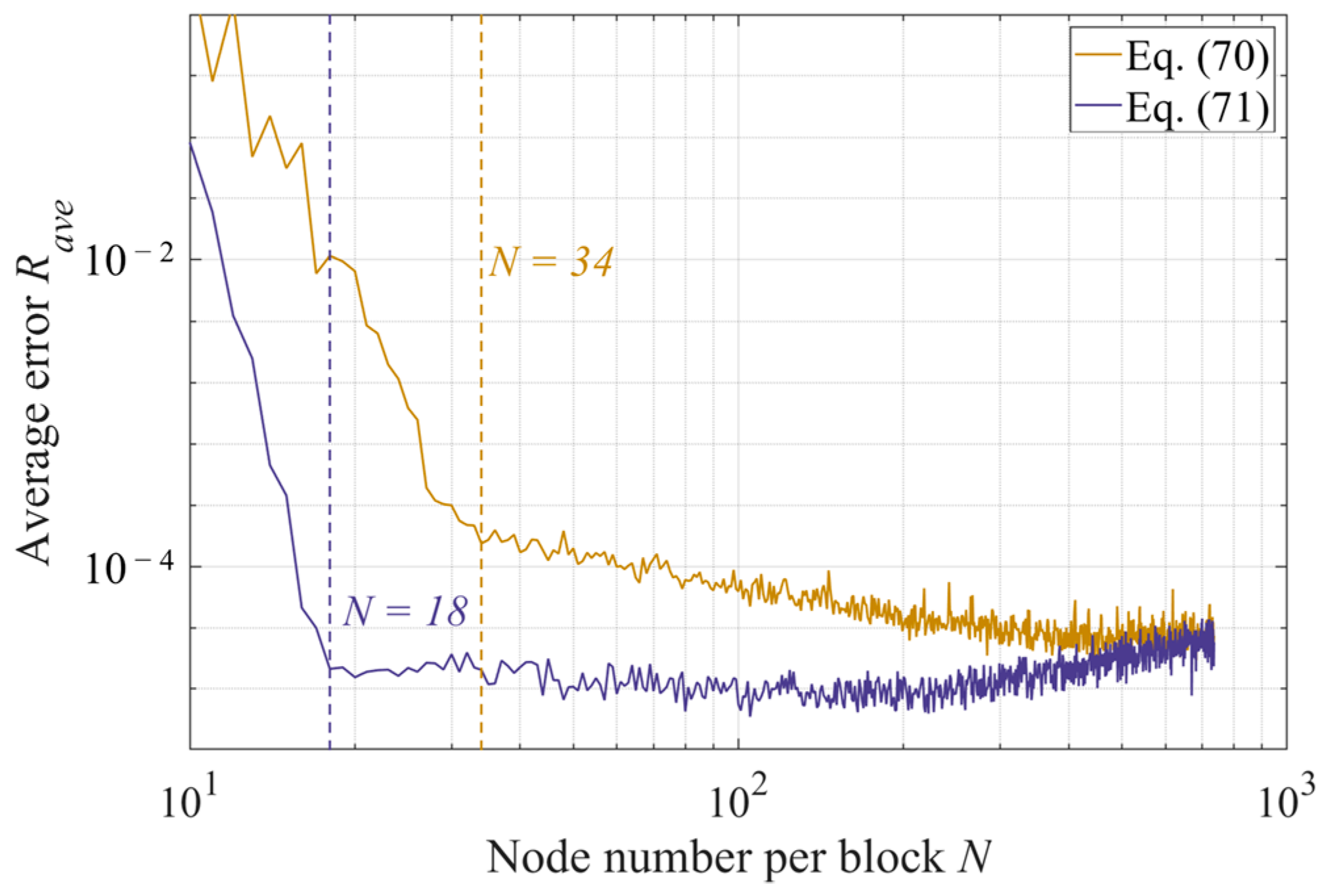
2.3. The Differential Quadrature Solution Scheme for Risers’ Parametric Vibration

According to the studies of previous researchers, the DQM is proved to be a powerful technique to solve the initial-value problems. Here, we will give a brief introduction to the DQM.

f(x) is a function in the domain of [a, b] with nth order continuous derivatives with respect to x. According to the Lagrange interpolation formula, f(x) could be approximated to a weighted summation:

$$f\left(x\right)\cong {\displaystyle \sum _{k=1}^K{\lambda }_k\left(x\right)f\left(x_k\right)}.$$

(33)

where

$${\lambda }_k\left(x\right)={\displaystyle \prod _{m=1,m\ne k}^K\left(\frac{x-x_k}{x_m-x_k}\right)}.$$

(34)

Thus, the nth order derivative of f(x) can also be approximated to the derivative of this interpolation function:

$$\frac{{\mathrm{d}}^{n}f\left(x\right)}{\mathrm{d}{x}^n}\cong {\displaystyle \sum _{k=1}^K\frac{{\mathrm{d}}^n{\lambda }_k\left(x\right)}{\mathrm{d}{x}^n}f\left(x_k\right)}.$$

(35)

If {x_k} are given nodes, the derivatives of f(x) on these given nodes can be expressed as

$${\left(\frac{\mathrm{d}f\left(x\right)}{\mathrm{d}x}\right)}_{x=x_l}\cong {\displaystyle \sum _{k=1}^K{A}_{kl}f\left(x_k\right)},$$

(36)

$${\left(\frac{{\mathrm{d}}^{2}f\left(x\right)}{\mathrm{d}{x}^2}\right)}_{x=x_l}\cong {\displaystyle \sum _{k=1}^K{B}_{kl}f\left(x_k\right)},$$

(37)

where

$$A_{kl}={\left(\frac{\mathrm{d}{\lambda }_k\left(x\right)}{\mathrm{d}x}\right)}_{x=x_l},$$

(38)

$$B_{kl}={\left(\frac{{\mathrm{d}}^2{\lambda }_k\left(x\right)}{\mathrm{d}{x}^2}\right)}_{x=x_l}.$$

(39)

With this interpolation and derivation scheme, the value of f(x) and its derivatives can be expressed with weighted summations of the function values at several discrete nodes. Sherbourne and Pandey [25] found that the DQ solution is very sensitive to the node spacing. Runge’s phenomenon may easily occur when the nodes are uniformly distributed. Thus, the Chebyshev node spacing scheme is utilized:

$${\tau }_k={\tau }_1+\frac{1}{2}\left[1-\cos \left(\frac{k-1}{K-1}\pi \right)\right]\left({\tau }_K-{\tau }_1\right), k =1,2,3,\dots ,K.$$

(40)

Then, q_i and its derivatives on these node points could be expressed as

$$q_{il}=q_i\left({\tau }_l\right)={\displaystyle \sum _{k=1}^K{E}_{kl}{q}_{ik}},$$

(41)

$$q_{il}{}^{\prime }={\displaystyle \sum _{k=1}^K{A}_{kl}{q}_{ik}},$$

(42)

$${q_{il}}^{″}={\displaystyle \sum _{k=1}^K{B}_{kl}{q}_{ik}},$$

(43)

where

$$E_{kl}=\{\begin{array}{l}1,(k=l)\\ 0,(k\ne l)\end{array}.$$

(44)

Substituting Equations (41)–(43) to Equation (26),

$$\begin{array}{l}{\displaystyle \sum _{i=1}^I{\displaystyle \sum _{k=1}^K[ ][E_{ij}{B}_{kl}+\left({\alpha }_j{E}_{ij}+{\beta }_j{E}_{ij}\cos 2{\tau }_l\right)E_{kl}+\zeta E_{ij}{A}_{kl}}}\\ +\left({\mu }_1{P}_{ij}{E}_{kl}+{\mu }_2{Q}_{ij}{E}_{kl}+{\mu }_3{Q}_{ij}{A}_{kl}\right)+{\mu }_4{\gamma }_j{E}_{ij}{E}_{kl}]q_{ik}=H_{jl}\end{array}; j=1,2,3,\dots ,I; l=1,2,3,\dots ,K$$

(45)

where

$$H_{jl}=H_j\left({\tau }_l\right).$$

(46)

In Equation (45), index i is the order number, and index k represents the node number of dimensionless time coordinate τ. The discretized differential equation is obtained by using Equation (45), but the equation is underdetermined if the boundary conditions are not given [37]. To avoid the right end of Equation (45) to be constant at zero, the initial value for each mode is given as 0.001, namely

$$q_j\left({\tau }_1\right)=0.001, j=1, 2, 3, \dots , I.$$

(47)

The initial velocity of each mode is set to zero:

$$q_j{}^{\prime }\left({\tau }_1\right)=0, j=1, 2, 3, \dots , I.$$

(48)

In discretized form,

$${\displaystyle \sum _{i=1}^I{\displaystyle \sum _{k=1}^K{E}_{ij}{E}_{kl}{q}_{ik}}}=0.001; l=1; j=1, 2, 3, \dots , I;$$

(49)

$${\displaystyle \sum _{i=1}^I{\displaystyle \sum _{k=1}^K{E}_{ij}{A}_{kl}{q}_{ik}}}=0; l=1; j=1, 2, 3, \dots , I.$$

(50)

The initial condition can be embedded to the discretized differential equation set Equation (45) by replacing the equations of index l = 1, N with Equations (49) and (50). However, such a replacement would raise the problem that the properties at these replaced indexes will be overlooked. According to [26,27,38], adjacent δ points can be arranged, and the mechanical properties of these replaced points can be approximated by those of adjacent δ points. Additionally, the closeness between the adjacent point and the replaced point is usually set to be of the order δ = 10⁻⁵. Thus, the Chebyshev node spacing scheme Equation (40) should be reorganized with adjacent δ points:

$$\begin{array}{l}{\tau }_1=0,\hspace{0.17em}{\tau }_2=\delta ,\hspace{0.17em}{\tau }_{K-1}=1-\delta ,\hspace{0.17em}\hspace{0.17em}{\tau }_K=1;\delta ={10}^{-5};\\ {\tau }_k={\tau }_2+\frac{1}{2}\left[1-\cos \left(\frac{k-1}{K-1}\pi \right)\right]\left({\tau }_{K-1}-{\tau }_2\right),k=3,\dots .,K-2.\end{array}$$

(51)

As mentioned in many previous works, for a large number of node points and a large-ordered algebraic equation system, the matrix of DQM will be ill-conditioned [37,39]. However, for the current problem, a large number of node points is needed to acquire a long-time scope numerical solution. Thus, the block-marching technique [39] is introduced to overcome such conflict between the long-time solution and the ill-conditioned matrix. As the level-by-level solution scheme in R–K schemes, the block-marching of DQM divides the temporal problem domain into a sequence of blocks, and the solving procedure is organized block-by-block, which means the initial conditions of each lateral block are determined by the solution of the former block, as shown in Figure 3. For instance, the solution of $q_i$ in the first block $\tau =\left[0,T\right]$ can be solved by Equations (45), (49), and (50). For the second block where $\tau =\left[T,2T\right]$, the initial conditions can be defined with the q and q′ values on the last node of the first block, and the equation set of the second block can be expressed as

$$\begin{array}{l}{\displaystyle \sum _{i=1}^I{\displaystyle \sum _{k=K}^{2K-1}[E_{ij}{B}_{kl}+\left({\alpha }_j{E}_{ij}+{\beta }_j{E}_{ij}\cos 2{\tau }_l\right)E_{kl}+\zeta E_{ij}{A}_{kl}}}\\ +\left({\mu }_1{P}_{ij}{E}_{kl}+{\mu }_2{Q}_{ij}{E}_{kl}+{\mu }_3{Q}_{ij}{A}_{kl}\right)+{\mu }_4{\gamma }_j{E}_{ij}{E}_{kl}]q_{ik}=H_{jl}\end{array}; j=1,2,\dots ,I; l=K+1,K+2,\dots ,2K-2$$

(52)

$${\displaystyle \sum _{i=1}^I{\displaystyle \sum _{k=K}^{2K-1}{E}_{ij}{E}_{kl}{q}_{ik}}}=q_{jK}; j=1, 2, 3, \dots , I; l=K;$$

(53)

$${\displaystyle \sum _{i=1}^I{\displaystyle \sum _{k=K}^{2K-1}{E}_{ij}{A}_{kl}{q}_{ik}}}={q^{\prime }}_{jK}={\displaystyle \sum _{i=1}^I{\displaystyle \sum _{k=1}^K{E}_{ij}{A}_{k\left(K\right)}{q}_{ik}}}; =1, 2, 3, \dots , K; l=2K-1.$$

(54)

Similarly, the sequential blocks can be solved by this block-marching scheme.

2.4. Analytical Solution for Mathieu Instability

According to the Floquet theory [40], we have the the Mathieu equation:

$$q^{″}\left(\tau \right)+\left(\alpha +\beta \cos 2\tau \right)q\left(\tau \right)=0$$

(55)

having a pair of solution basis

$$\{\begin{array}{l}{q}_1\left(\tau \right)={\sigma }_1^{\tau /\pi }{p}_1\left(\tau \right)\\ q_2\left(\tau \right)={\sigma }_2^{\tau /\pi }{p}_2\left(\tau \right)\end{array},$$

(56)

where p₁ and p₂ are periodic functions with period π, and σ₁ and σ₂ are complex coefficients. Additionally, σ₁ and σ₂ are the roots of the quadratic Equation [40]:

$${\sigma }^2-2a\sigma +1=0,$$

(57)

namely,

$${\sigma }_{1,2}=a\pm \sqrt{a^2-1}.$$

(58)

When |a| < 1, both σ₁ and σ₂ are complex roots with modulus 1, and the solution of Equation (56) is stable with respect to τ. On the contrary, when |a| > 1, moduli of σ_1,2 are bigger than 1, and that means the solution of Equation (56) is unstable. For the situation |a| = 1, both σ₁ and σ₂ are equal to 1 or −1, and the solution of Equation (56) is periodic with period π or 2π. Therefore, |a| = 1 is the critical condition between the stable regions and unstable regions, and it means that for the cases at the critical edge between stable and unstable regions, the solutions for Equation (56) are periodic functions with period π or 2π.

To obtain the borderlines of the unstable region, firstly, we assume the solutions to be with period π. Thus, the assumed solution could be expanded with the Fourier series:

$$q\left(\tau \right)={\displaystyle \sum _{n=0}^{\infty }{a}_n\cos \left(2n\tau \right)}+{\displaystyle \sum _{n=1}^{\infty }{b}_n\sin \left(2n\tau \right)}.$$

(59)

Substituting Equation (59) into Equation (55),

$$\begin{array}{l}{\displaystyle \sum _{n=0}^{\infty }\left(\alpha -4n^2\right)a_n\cos \left(2n\tau \right)}+{\displaystyle \sum _{n=1}^{\infty }\left(\alpha -4n^2\right)b_n\sin \left(2n\tau \right)}\\ +\beta \cos \left(2\tau \right)\left[{\displaystyle \sum _{n=0}^{\infty }{a}_n\cos \left(2n\tau \right)}+{\displaystyle \sum _{n=1}^{\infty }{b}_n\sin \left(2n\tau \right)}\right]=0\end{array}$$

(60)

Using the prosthaphaeresis rules,

$$\{\begin{array}{l}\cos \left(2\tau \right)\cos \left(2n\tau \right)=\frac{1}{2}\left[\cos \left(2n+2\right)\tau +\cos \left(2n-2\right)\tau \right]\\ \cos \left(2\tau \right)\sin \left(2n\tau \right)=\frac{1}{2}\left[\sin \left(2n+2\right)\tau +\sin \left(2n-2\right)\tau \right]\end{array}.$$

(61)

According to the orthogonality the trigonometric functions,

$$\{\begin{array}{l}{\displaystyle {\int }_0^{\pi }\cos \left(2n\tau \right)\cos \left(2m\tau \right)d\tau }=\{\begin{array}{l}0,m\ne n\\ \pi /2,m=n\end{array}\\ {\displaystyle {\int }_0^{\pi }\sin \left(2n\tau \right)\cos \left(2m\tau \right)d\tau }=0\end{array}, m=1, 2, 3, \dots ,$$

(62)

and

$$\{\begin{array}{l}{\displaystyle {\int }_0^{\pi }\cos \left(2n\tau \right)\sin \left(2m\tau \right)d\tau }=0\\ {\displaystyle {\int }_0^{\pi }\sin \left(2n\tau \right)\sin \left(2m\tau \right)d\tau }=\{\begin{array}{l}0,m\ne n\\ \pi /2,m=n\end{array}\end{array}, m=1, 2, 3, \dots .$$

(63)

Substituting Equation (61) into Equation (60), and integrating this equation multiplied with weight function cos(2mτ) from 0 to π, a group of linear equation set is formed:

$$\left[\begin{array}{cccccc}\alpha & \beta /2& 0& 0& 0& \cdots \\ \beta & \alpha -4\times 1^2& \beta /2& 0& 0& \cdots \\ 0& \beta /2& \alpha -4\times 2^2& \beta /2& 0& \cdots \\ 0& 0& \beta /2& \alpha -4\times 3^2& \beta /2& \cdots \\ ⋮& ⋮& ⋮& \ddots & \ddots & \ddots \end{array}\right]\left[\begin{array}{c}{a}_0\\ a_1\\ a_2\\ a_3\\ ⋮\end{array}\right]=\left[\begin{array}{c}0\\ 0\\ 0\\ 0\\ 0\end{array}\right].$$

(64)

Similarly, integrating the equation multiplied with weight function sin(2mτ):

$$\left[\begin{array}{cccccc}\alpha -4\times 1^2& \beta /2& 0& 0& 0& \cdots \\ \beta /2& \alpha -4\times 2^2& \beta /2& 0& 0& \cdots \\ 0& \beta /2& \alpha -4\times 3^2& \beta /2& 0& \cdots \\ 0& 0& \beta /2& \alpha -4\times 4^2& \beta /2& \cdots \\ ⋮& ⋮& ⋮& \ddots & \ddots & \ddots \end{array}\right]\left[\begin{array}{c}{b}_1\\ b_2\\ b_3\\ b_4\\ ⋮\end{array}\right]=\left[\begin{array}{c}0\\ 0\\ 0\\ 0\\ 0\end{array}\right].$$

(65)

To ensure the solution of Equation (59) is a constant 0 value, the determinant of the coefficient matrix of Equations (64) and (65) must be zero. Namely,

$$\left|\begin{array}{cccccc}\alpha & \beta /2& 0& 0& 0& \cdots \\ \beta & \alpha -4\times 1^2& \beta /2& 0& 0& \cdots \\ 0& \beta /2& \alpha -4\times 2^2& \beta /2& 0& \cdots \\ 0& 0& \beta /2& \alpha -4\times 3^2& \beta /2& \cdots \\ ⋮& ⋮& ⋮& \ddots & \ddots & \ddots \end{array}\right|=0,$$

(66)

or

$$\left|\begin{array}{cccccc}\alpha -4\times 1^2& \beta /2& 0& 0& 0& \cdots \\ \beta /2& \alpha -4\times 2^2& \beta /2& 0& 0& \cdots \\ 0& \beta /2& \alpha -4\times 3^2& \beta /2& 0& \cdots \\ 0& 0& \beta /2& \alpha -4\times 4^2& \beta /2& \cdots \\ ⋮& ⋮& ⋮& \ddots & \ddots & \ddots \end{array}\right|=0.$$

(67)

For cases where the solution of Equation (56) is of period 2π, there exist the eigen equations

$$\left|\begin{array}{cccccc}\alpha -1^2+\beta /2& \beta /2& 0& 0& 0& \cdots \\ \beta /2& \alpha -3^2& \beta /2& 0& 0& \cdots \\ 0& \beta /2& \alpha -5^2& \beta /2& 0& \cdots \\ 0& 0& \beta /2& \alpha -7^2& \beta /2& \cdots \\ ⋮& ⋮& ⋮& \ddots & \ddots & \ddots \end{array}\right|=0,$$

(68)

or

$$\left|\begin{array}{cccccc}\alpha -1^2-\beta /2& \beta /2& 0& 0& 0& \cdots \\ \beta /2& \alpha -3^2& \beta /2& 0& 0& \cdots \\ 0& \beta /2& \alpha -5^2& \beta /2& 0& \cdots \\ 0& 0& \beta /2& \alpha -7^2& \beta /2& \cdots \\ ⋮& ⋮& ⋮& \ddots & \ddots & \ddots \end{array}\right|=0.$$

(69)

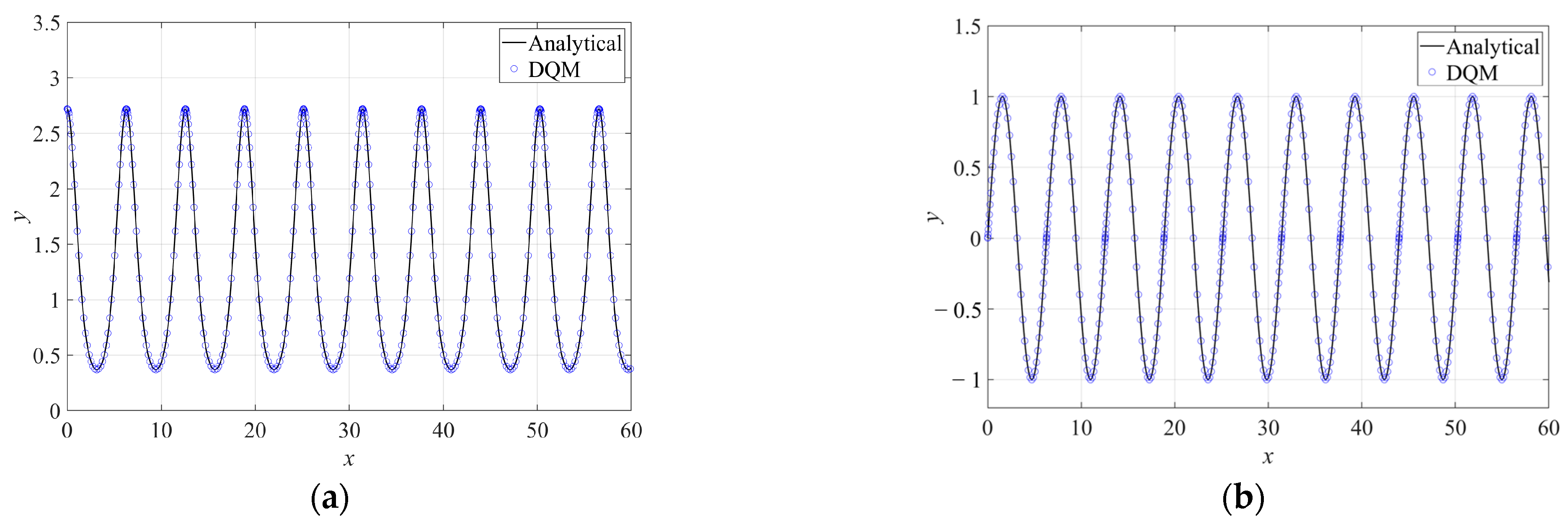
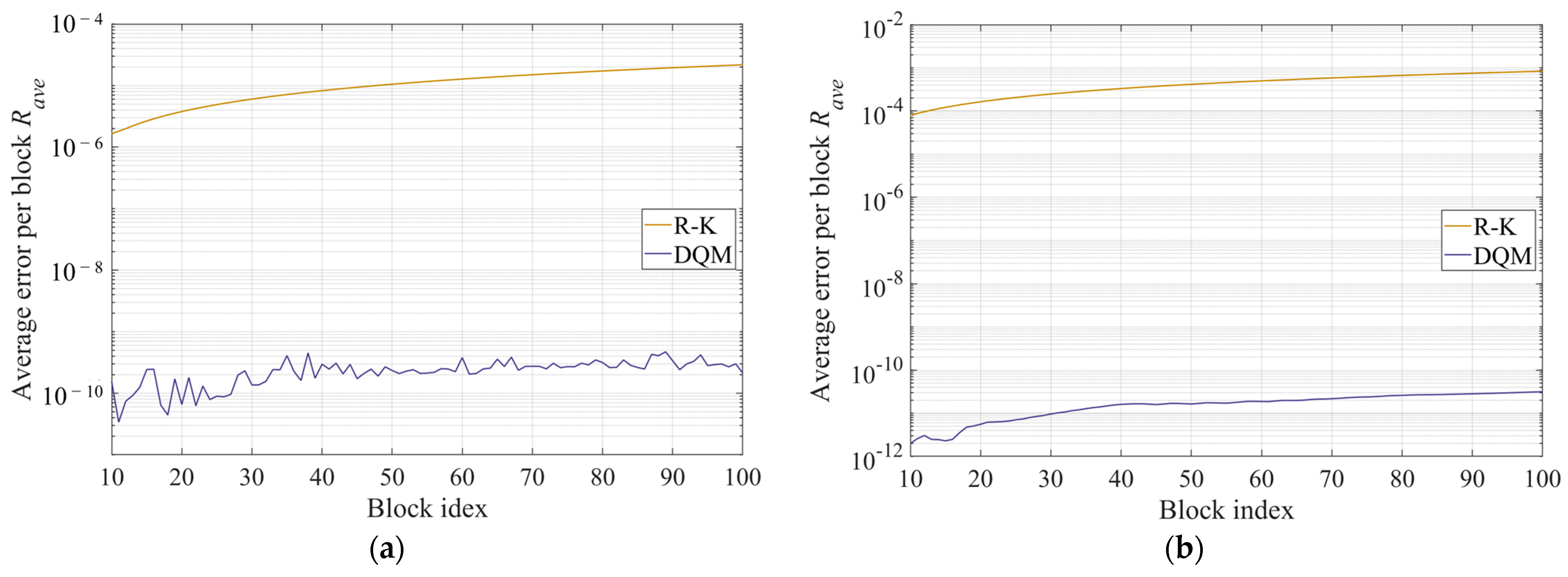
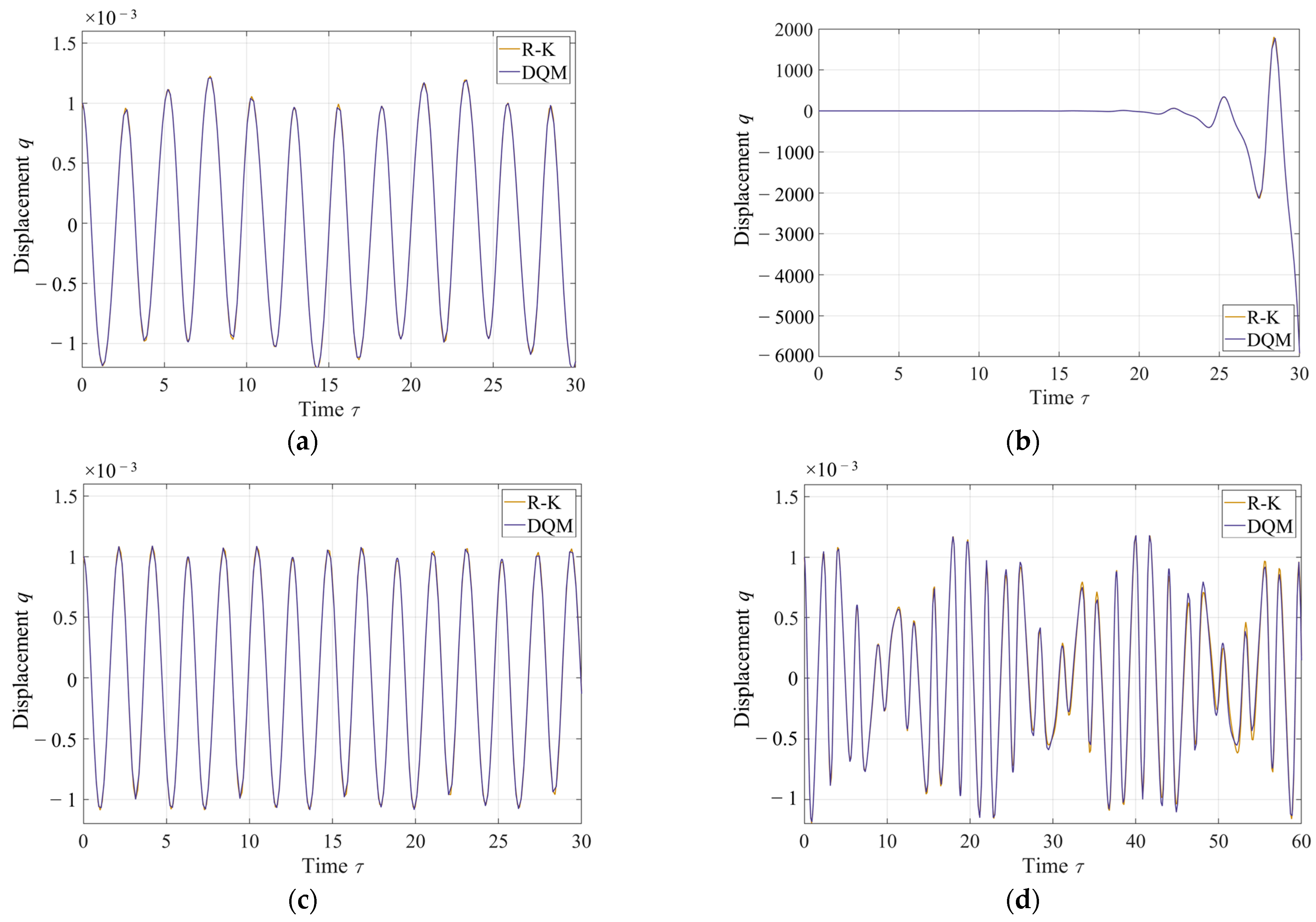
3. Verification and Validation of DQM

In this section, two simple equations, a first-order linear differential equation with harmonic coefficients and a second-order linear differential equation with constant coefficients, are considered:

$$y^{\prime }+\sin \left(x\right)y=0,\hspace{0.17em}y\left(0\right)=e,$$

(70)

and

$$y^{″}+y=0,\hspace{0.17em}y\left(0\right)=0,\hspace{0.17em}{y}^{\prime }\left(0\right)=1.$$

(71)

The analytical solutions of these equations can be expressed as

$$y=e^{\cos \left(x\right)}$$

(72)

for Equation (70), and

$$y=\sin (x)$$

(73)

for Equation (71).

As discussed in Section 2.3, the initial-value problems can be studied by the block-marching DQM. In the current solving scheme for these two equations, the computation domain $x\in \left[0,\hspace{0.17em}10\times 2\pi \right]$ is divided into 10 blocks with a length of 2π. Therefore, the long-time-scope initial problem of Equations (70) and (71) is divided into two sequences of short-time-scope subproblems that can be solved by DQM with a small number of nodes. Additionally, the DQM, whose node number N = 51, and analytical solutions for Equations (70) and (71) are given in Figure 4.

It can be acknowledged from Figure 4 that the solutions of DQM reach good agreements with those of the analytical solution. Furthermore, the convergence of DQM is evaluated with the average error

$$R_{ave}={\displaystyle \sum _{i=1}^{MN}\left|y_i-{\tilde{y}}_i\right|},$$

(74)

where $y_i$ is the analytical value and ${\tilde{y}}_i$ is the numerical value; M is the block number and, in the current examples, M is set to 10; N is the DQM node number of each block. Under such conditions, the average errors with different node numbers are computed and presented in Figure 5.

As shown in Figure 5, the average errors of both examples diminish sharply with the increase of node number per block when N remains in relatively small values. Additionally, when the node number exceeds a certain value, which is 34 for Equation (70) or 18 for Equation (71), the decreasing trend of the average errors falls to a relatively slight rate. However, when the node number increases further, the average error begins to alter in an increasing trend until at N = 737, the DQM solution scheme aborts because of the ill-conditioned matrix. Thus, in application practice, a relatively small node number is chosen in DQM. In the following study, 51 nodes are utilized in each block to form the DQM solution scheme.

According to the previous studies, the R–K method is a commonly utilized method in coping with the initial value problems. Here, the R–K solutions for Equations (70) and (71) are carried out to make a comparison with the DQM solutions. The R–K solution schemes in our study for Equations (70) and (71) are:

$$\{\begin{array}{l}{y}_1=e\\ y_{n+1}=y_n+\frac{h}{6}\left(K_1+2K_2+2K_3+K_4\right)\\ K_1=-\sin \left(x_n\right)y_n\\ K_2=-\sin \left(x_n+\frac{h}{2}\right)\left(y_n+\frac{h}{2}{K}_1\right)\\ K_3=-\sin \left(x_n+\frac{h}{2}\right)\left(y_n+\frac{h}{2}{K}_2\right)\\ K_4=-\sin \left(x_n+h\right)\left(y_n+h{K}_3\right)\end{array}$$

(75)

for Equation (70), and

$$\{\begin{array}{l}{y}_1=0\\ z_1=1\\ y_{n+1}=y_n+\frac{h}{6}\left(K_1+2K_2+2K_3+K_4\right)\\ z_{n+1}=z_n+\frac{h}{6}\left(L_1+2L_2+2L_3+L_4\right)\\ K_1=z_n,\hspace{1em}\hspace{1em}\hspace{1em}\hspace{0.17em}{L}_1=-y_n\\ K_2=z_n+\frac{h}{2}{L}_1,\hspace{0.17em}\hspace{0.17em}{L}_2=-\left(y_n+\frac{h}{2}{K}_1\right)\\ K_3=z_n+\frac{h}{2}{L}_2,\hspace{0.17em}\hspace{0.17em}{L}_3=-\left(y_n+\frac{h}{2}{K}_2\right)\\ K_4=z_n+h{L}_3,\hspace{1em}{L}_4=-\left(y_n+h{K}_3\right)\end{array}$$

(76)

for Equation (71).

The R–K solution scheme utilized in the current examples is an explicit single-step method. To ensure the same node number in each block as that in DQM, the step lengths for the current R–K schemes are:

$$h=\frac{2\pi }{N-1},N=51.$$

(77)

The solution of Equations (70) and (71) are solved by both DQM and R–K, and the average errors per block are evaluated and presented in Figure 6.

According to Figure 6, it can be informed that for these two examples the average error of the R–K method is much bigger than the DQM. That means with the same number of nodes the DQM could acquire more accurate solutions than the R–K. In addition, it can be told from the figures that the average error of the DQM for Equation (71) is smaller than Equation (70), while the trend of the R–K is the opposite. That means the causes of errors for these two methods are irrelevant.

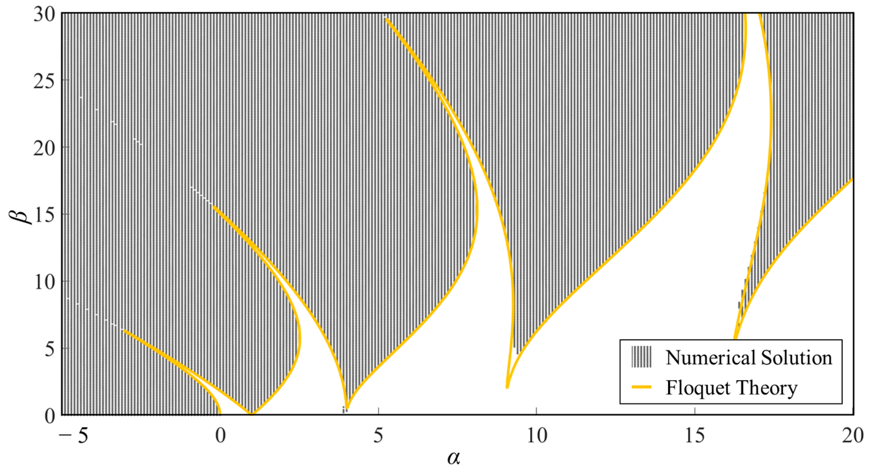
4. Instability Analysis of a Top-Tensioned Riser

4.1. DQM Solution for Mathieu Equation

In this section, the Mathieu equation (32) is considered. Additionally, the initial values for the current examples are:

$$\{\begin{array}{l}q\left(0\right)=0.001\\ q^{\prime }\left(0\right)=0\end{array}.$$

(78)

For specific values of α and β as listed in

Table 1. α and β values of four examples.

	Example 1	Example 2	Example 3	Example 4
α	6	6	9	9
β	2.2	8.8	2.2	8.8

, the accordingly time-domain solutions for the Mathieu equation are solved by both DQM and R–K, and the solutions are presented in Figure 7.

Firstly, according to Figure 7, the curves of DQM show good consistency with that of R–K, which is a vastly applied technique for the parametric vibrating problem. Additionally, it can be easily told from the figures that for Examples 1, 2, and 4, the solutions for the Mathieu equation are stable; however, for Example 2, the solution is divergent with respect to time τ. Following such logic, a series of Mathieu equation examples with α ranging from −5 to 20 and β ranging from 0 to 30 are calculated by this DQM solution scheme to form the instability chart of the Mathieu equation. When it comes to how to tell whether an example is divergent, we set up a verification scheme as follows:

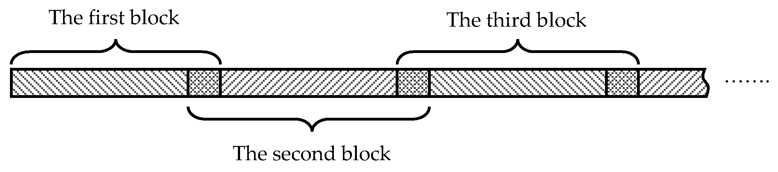
• Separate the long-time-scope solutions into blocks with lengths of 2π;
• Extract the maximum of each block;
• Compare the maxima between every neighboring block, and if the maximum is increasing block by block, we define the solution for the current example as divergent;
• For the examples that fail the test in step three, calculate the ratio of the maximum of the last block and that of the initial block, and if the ratio is bigger than 100, we define the solution for the current example as divergent; otherwise, it is defined as convergent.

For the solutions defined as divergent, we mark the corresponding (α, β) point in the α-β plane. Thus, after all of the verification schemes of every example are considered, a map of the instability chart for the Mathieu equation is acquired. Additionally, this instability chart is acquired via the aforementioned scheme as well as the borderline solved by Equations (62)–(65) and is depicted in Figure 8.

As is shown in Figure 8, the instability region acquired by the DQM fits well with the borderline defined by the Floquet theory. Therefore, it can be easily concluded that the DQM is a suitable method to evaluate the parametric vibration problems of risers. In the following sections, the parametric instability of risers under different conditions will be discussed with the solutions of the DQM.

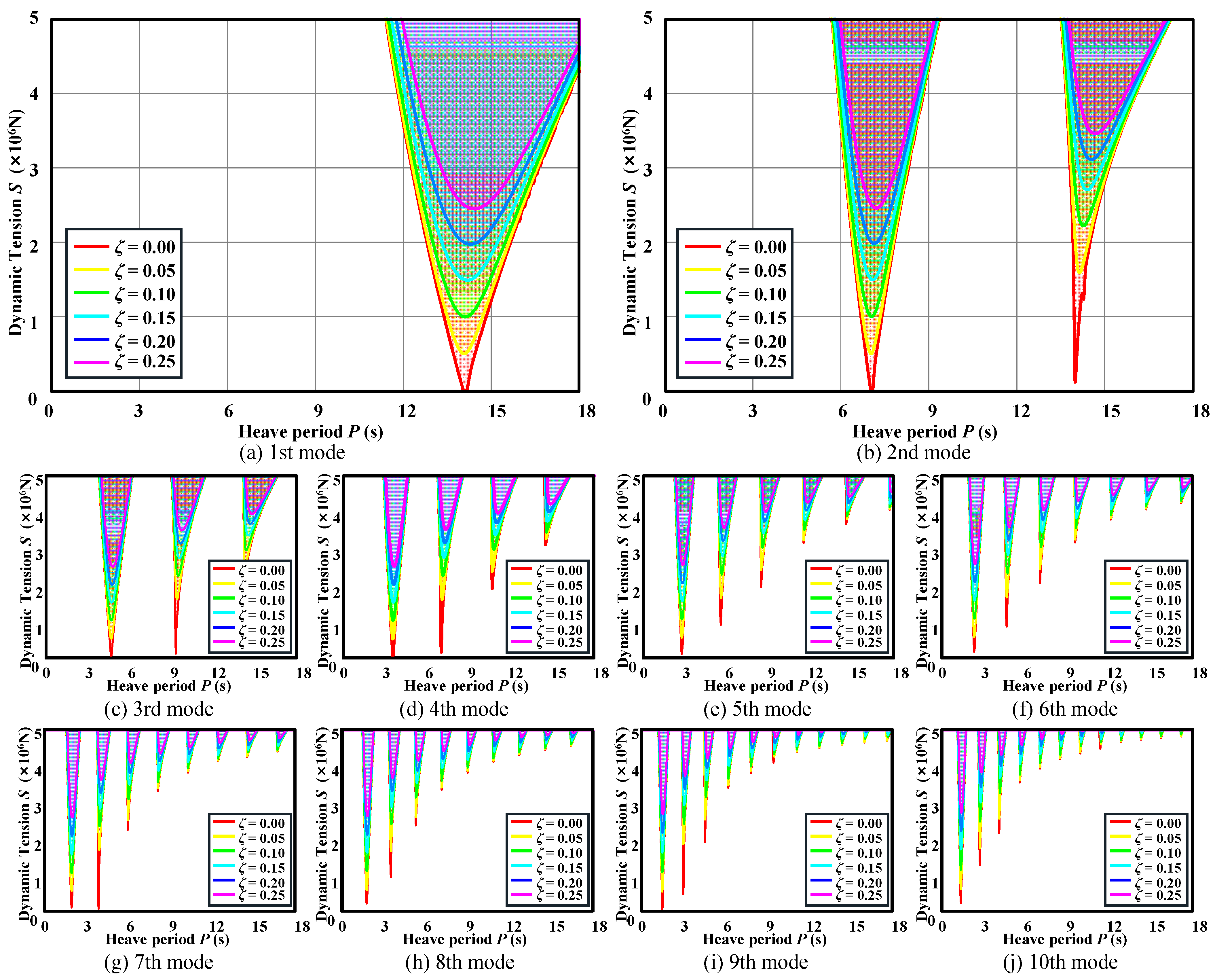
4.2. Instabilities of Risers with Different Damping Coefficients

In this section, the parametric instability of a top-tensioned riser with different damping coefficients is discussed through the solutions of the DQM. Additionally, the riser we study is modified from a mini-TLP in the Gulf of Mexico [11] whose major parameters are listed in

Table 2. Major parameters of the top-tensioned riser and the environment.

Items	Symbols	Values
Young’s modulus	E	210 GPa
Sea water density	ρw	1025 kg/m3
Pipe wall density	ρs	7850 kg/m3
Internal fluid density	ρf	800 kg/m3
Pipe’s outer diameter	D	0.66 m
Pipe’s Length	h	0.026 m
Static Tension of the riser	T0	5 × 107 N

. The internal flow velocity U and wet-weight coefficients k_mw are set to zero, which means that the fluid inside the pipe is assumed to be still, and the weight of the riser unit and the buoyancy provided by the tanks are assumed to be compensating for each other. The parametric excitation is defined through T_d(t) = Scos(2πt/P), where the amplitude S ranges from 0 to 5 × 10⁶ N and the period P ranges from 0 to 18s. Therefore, the instability charts of six different damping coefficients ζ = (0.00, 0.05, 0.10, 0.15, 0.20, 0.25) are acquired and are presented in Figure 9.

Because the coupling terms μ₁P_ijq_i, μ₂Q_ijq_i, and μ₃Q_ijq_i’ are set to zero, there are no coupling effects between different modes. As a result, the parametric instabilities of different modes are independent of each other. In Figure 9, the instability regions of different damping coefficients of the first ten orders are presented. The instability regions are represented with translucent shades confined to the solid borderlines. It can be told from the pictures that with the increase of damping coefficients, the shaded areas move upwards accordingly. It means that the risers with larger damping coefficients are less prone to vibrate unstably Besides, at a specific heave period, stronger dynamic tension amplitude is needed to induce the parametric instability of the riser.

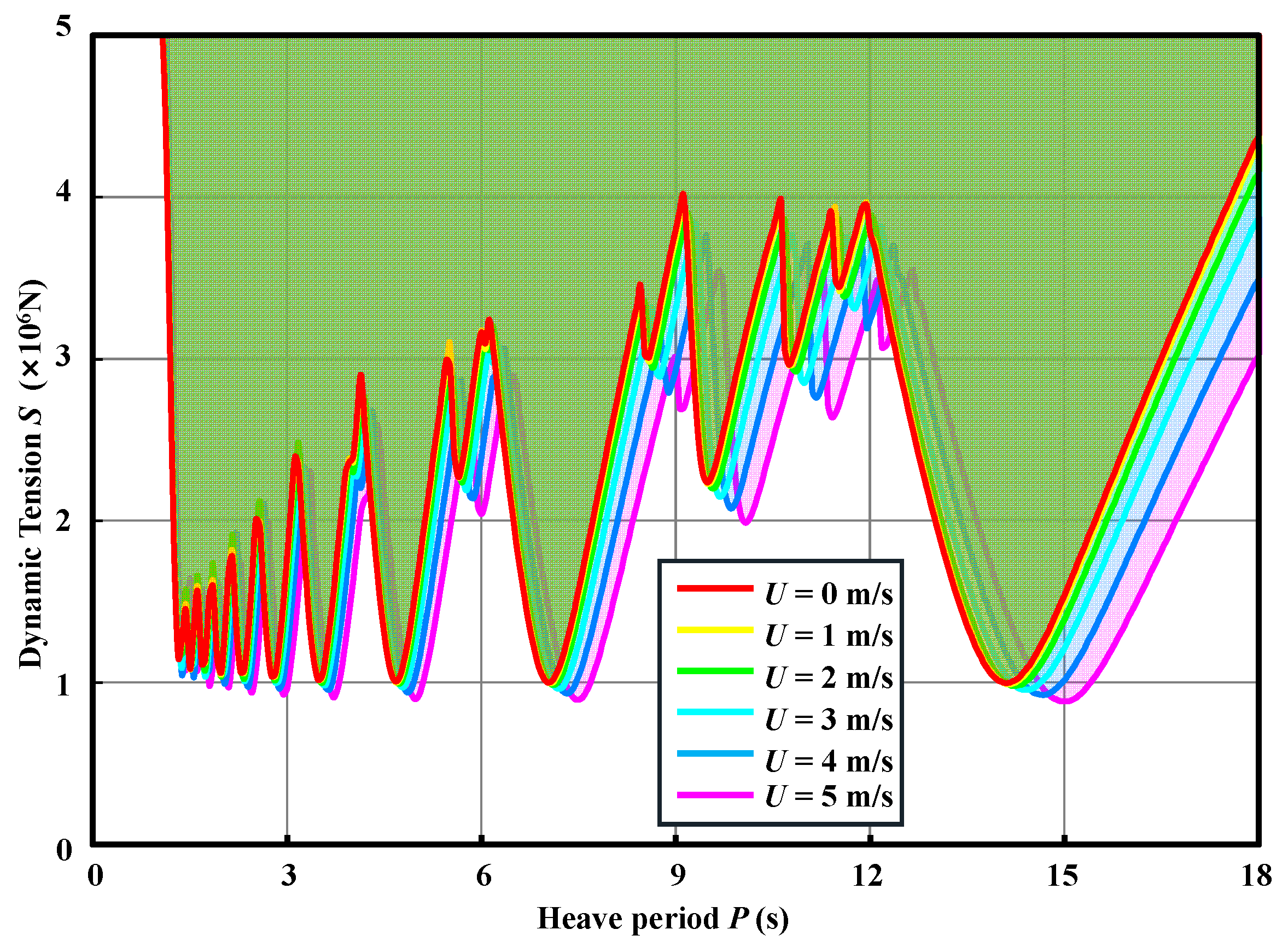
4.3. Instabilities of Risers with Different Internal Flow Velocity

According to Chen’s [1,2,3,4] research, the velocity of the internal flow will alter the vibrating characters of the pipe. Due to the role of the risers being to transport fluid from seabed to the platform, in this section, the instabilities of the riser with different internal flow velocities are studied. The parameters of the riser and the environment are listed in Table 2. The damping coefficient ζ is set to 0.1, and the wet-weight coefficient k_mw is set to zero. The instability charts of different internal flow velocities U, which range in array [0–5] m/s, are obtained and depicted in Figure 10.

The existence of the nonzero coupling term μ₃Q_ijq_i’ would induce interferences between different modes. Therefore, when one order of the modes vibrates unstably, the divergent response of the current mode will gradually trigger other modes to vibrate unstably. Namely, when the internal flow velocity is not equal to zero, the μ₃Q_ijq_i’ term would take effect crossing different modes. For instance, in case the first mode of the riser vibrates unstably in the shape of $\sin \left(\frac{\pi z}{L}\right)$, the divergent vibration of the first order would pump continuous excitations to other modes because of the existence of the coupling term μ₃Q_ijq_i’. Thus, the parametrically unstable vibrations of other modes will be triggered. Therefore, the parametrical instabilities of different modes are coexistent, and such an instability chart will no longer be presented individually by mode. In Figure 10, it could be found that with the increase of internal flow velocity, the unstable regions move towards the bottom right. It can be informed that when the internal flow velocity increases, the risers are more easily to be parametrically unstable, and the minimal dynamic tension that could induce the parametric instability would decrease accordingly. Besides, it can also be spotted that the movement of the unstable borderline is accelerating with the increase of internal flow velocity. The acceleration phenomenon is due to the coefficient μ₄, which is proportional to U². Thus, the influence of the internal flow velocity on the riser’s parametric instability is small at a low-frequency range where U is less than 2 m/s, while its influence would reach a considerable extent otherwise.

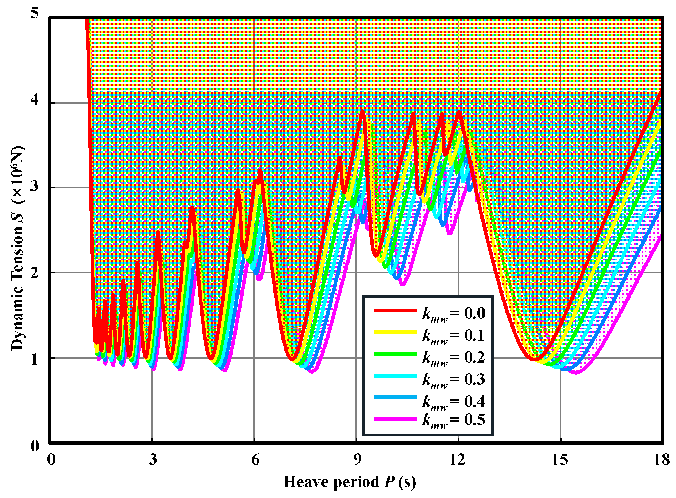
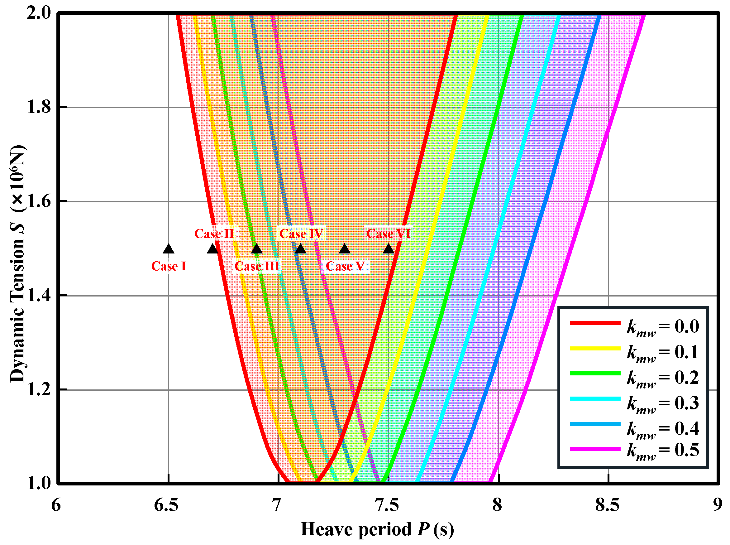
4.4. Instability of Risers with Different Wet-Weight Coefficients

According to the governing equation Equation (29), the terms α_jq_j, μ₁P_ijq_i, and μ₂Q_ijq_i, which are relative to the unit wet weight, are considered. Thus, the influences of wet weight on risers’ parametric instability are unavoidable. Since the unit wet weight can be adjusted by changing the size of buoyancy tanks distributed along with the risers, a dimensionless coefficient k_mw is used in our research to control the unit wet weight. In this section, a series of parametric vibration examples is set up focusing on the riser defined in Table 2 with damping ζ = 0.1 and internal flow velocity U = 2 m/s, and the time-domain vibrating solution is calculated through the DQM. After that, the parametric instability charts of the aforementioned model are obtained and depicted in Figure 11.

With the solutions shown in Figure 11, it can be easily inferred that when the wet-weight coefficient increases, the instability region of the riser’s parametric vibration moves towards the bottom right. Thus, it can be concluded that the increase of wet-weight coefficients will decrease the minimum dynamic tensions S, which means the parametric resonance will occur more easily. In addition, it can be inferred that longer excitation periods are needed to induce the risers’ parametric resonance for models with larger wet-weight coefficients. Being different from the acceleration phenomenon of the influence of the internal flow velocity, the alteration of the unstable region is uniform with the increase of the wet-weight coefficient. This is because the coefficients α_j, μ₁ and, μ₂ are linearly related to wet weight m_w, while the U-dependent coefficient μ₄ is quadratically related to the internal flow velocity.

5. Dynamic Responses of Risers’ Parametric Vibration

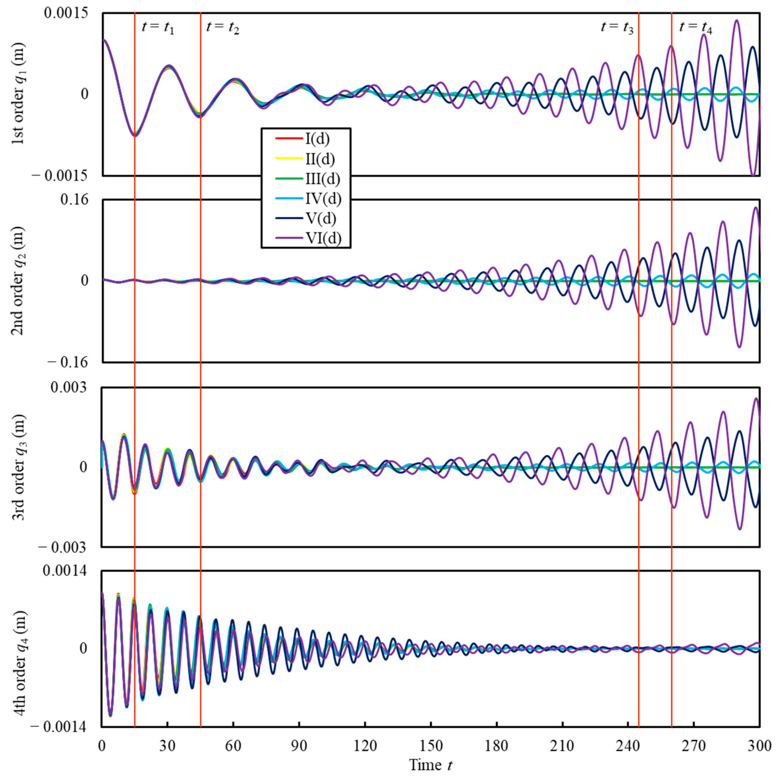
5.1. The Dynamic Response of Different Excitation Periods

In this section, the responses of different cases are considered. Firstly, we discuss the responses of a riser with wet-weight coefficient k_mw = 0.3 subjecting to parametric excitations of different periods, and the detailed parameters for these cases are listed in

Table 3. Detailed parameters of different cases.

Parameter	Case I(d)	Case II(d)	Case III(d)	Case IV(d)	Case V(d)	Case VI(d)
ζ	0.1
U	2 m/s
kmw	0.3
S	1.5 × 106 N
P	6.5 s	6.7 s	6.9 s	7.1 s	7.3 s	7.5 s

.

According to the instability chart shown in Figure 12, which is excerpted from Figure 11, the Cases I(d)–III(d) are located at the stable region of the riser with k_mw = 0.3 (the cyan instability borderline), while the Cases IV(d)–VI(d) are located at the unstable region. Additionally, the response solutions of the first four modes of these cases are presented in Figure 13.

According to the response solutions shown in Figure 13, it can be informed that the solutions of Cases I(d)–III(d) are convergent while the responses of the other cases are divergent with respect to time. For the unstable cases (i.e., Cases IV(d)–VI(d)), the time-domain weight function of the second order q₂ fluctuates with a growing amplitude, while the fluctuating amplitudes of other modes are decreasing at the beginning and start to increase starting at a certain time. It also can be observed that the divergent speed of the second mode is much faster than other modes as it is shown that the vibrating amplitude of Case VI(d) at t = 300s of the second reaches 0.05 m, while the vibrating amplitude at t = 300s of other modes is no more than 0.005 m. This is because Cases IV(d)–VI(d) lie in the second order parametric unstable region. Thus, the instability of the second mode is stimulated by the parametric excitation initially. Whereafter, as the existence of the coupling effect between different modes, the vibration of other modes begins to diverge with the growth of the vibrating amplitude of the second mode. In Figure 13, we draw two transversal lines at t = t₁ and t = t₂. Observing the time-domain responses between t₁ and t₂, it can be informed that there is only one waveform between these two time-points in the solution of the first order, while there are three waveforms in the third order and four waveforms in the fourth order, regardless of the change of excitation period. This is because for the first, third and fourth modes, the free vibration takes a major part of the responses at the beginning before the coupling effect induced by the parametric resonance of the second mode takes effect. When observing the responses in the amplitude-increasing phase, it can be found that there exist slight phase differences between different cases, and these phase differences can be spotted with their accumulation with the increase of time. Moreover, when observing the responses between t = t₃ and t = t₄, it can be seen that there is only one waveform for Case VI, regardless of which mode it is. The cause of these phenomena is that the free vibrations die down with the passing of time and the coupling effect induced by the second-order parametric resonance, whose period is related to the excitation period, gradually takes the major part. Thus, the response solutions of different modes vibrate with the same period as the second-order parametric resonance.

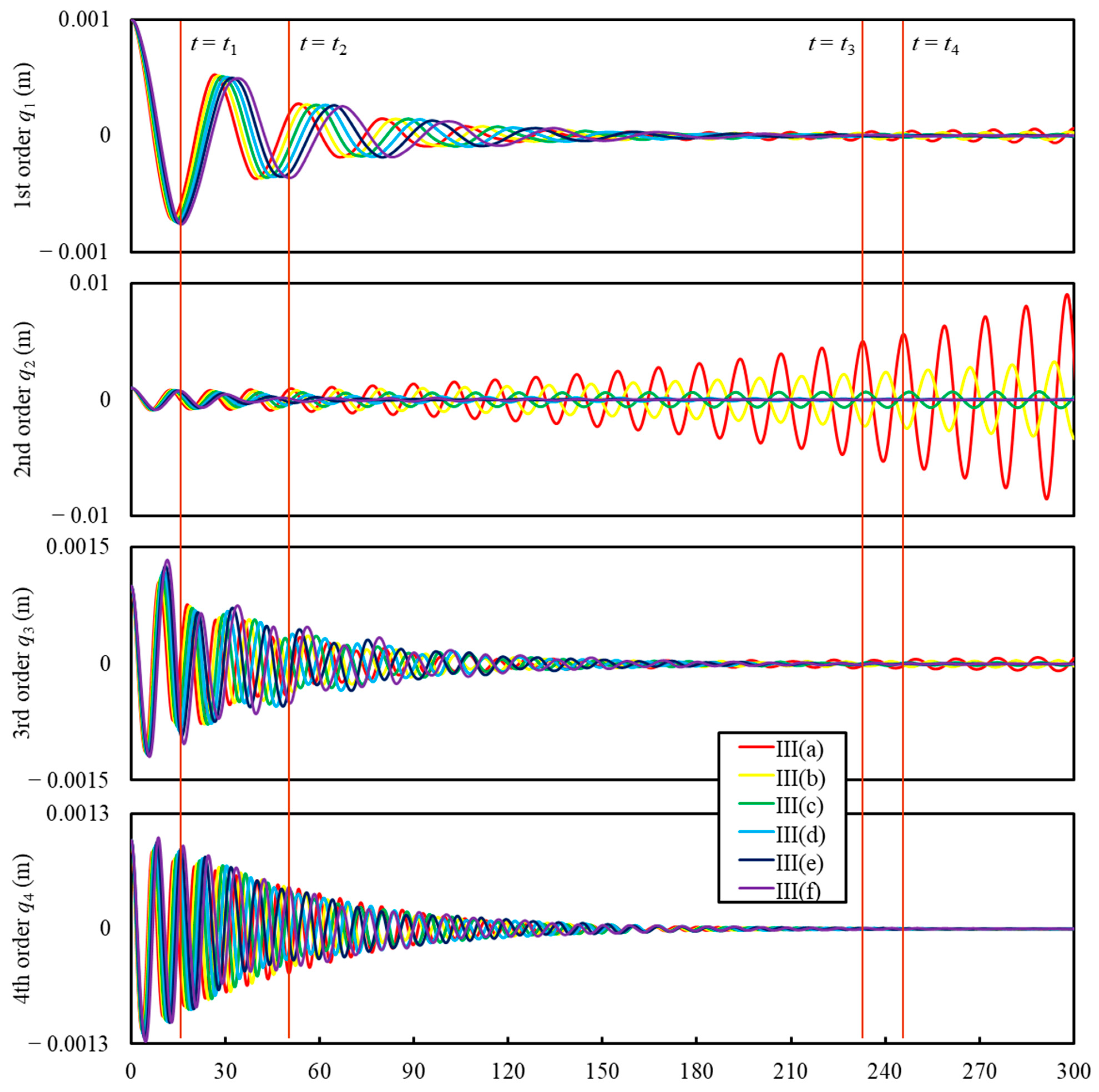
5.2. The Dynamic Response of Different Wet-Weight Coefficients

To study the influence of wet weight on risers’ parametric vibration responses, we set a series of cases with different wet-weight coefficients, as listed in

Table 4. Detailed parameters of different cases.

Parameter	Case III(a)	Case III(b)	Case III(c)	Case III(d)	Case III(e)	Case III(f)
ζ	0.1
U	2 m/s
kmw	0.0	0.1	0.2	0.3	0.4	0.5
S	1.5 × 106 N
P	6.9 s

. The response solutions of these cases are solved with DQM and presented in Figure 14.

In Figure 14, the responses of the first four orders of the six cases listed in Table 4 are illustrated. According to the response solution of the second order q₂, it can be assumed that the vibrating amplitude of the second order responses of Cases III(a)–III(b) are increasing with the time, and those of Case III(c) are keeping stable, while those of Cases III(d)–III(f) are decreasing. The convergences of these six cases are consistent with the prediction of the instability chart Figure 12, that the mark of Case III lies in the unstable region of the instability regions of k_mw = 0.0 and 0.1, and on the edge of the instability region of k_mw = 0.2, but out of the instability regions of k_mw = 0.3, 0.4, and 0.5.

For the first, third, and fourth orders of the modes, the response amplitudes decrease initially. Due to the coupling effect between modes, the divergence of the second-order excites the first and third mode to vibrate divergently from a certain time. At the decreasing phase of the responses where time t is between t₁ and t₂, the vibrating period is altered in accordance with the wet-weight coefficient. For a bigger wet-weight coefficient, the free vibrating period increases. However, for the time between t₃ and t₄, the free vibrations die down, and the parametric resonance takes the main part of the responses. At this phase, the vibrating periods of different modes reach an agreement. Additionally, these phenomena can tell that the alteration of the wet-weight coefficients will change the period of free vibration but have little effect on the period of parametric vibration.

6. Conclusions

In the current work, the parametrical vibration problem of risers has been considered. The governing equation of parametrically excited risers is deduced. Moreover, the DQM is applied to Galerkin’s reduced form of this equation to study the parametric vibration problem of the risers. By testing this solution scheme in two simple equations, the accuracy of the DQM method is evaluated. With the good consistency between the DQM and the R–K for the Mathieu equation, the competency of the DQM in risers’ parametric vibration problem has been verified.

According to the numerical experiments on risers with different parameters, some important conclusions can be drawn as follows:

• The instability charts are given by both DQM fitting well and with the borderlines given by the Floquet theory.
• Increasing damping can control the parametric resonance from occurring.
• The increase of internal flow velocity and the wet-weight coefficients will deteriorate the parametric instability of the riser. Additionally, the influences of internal flow velocity on risers’ parametric instability are nonlinear, while the those of wet weight are linear.
• According to the response solutions, the existence of the coupling term will give a chance to the parametrically unstable modes to excite other modes to vibrate unstably.
• The alteration of the parametric excitation period will not change the period of free vibration, while the excitation period will have an effect on the parametrically vibrating period.
• The alteration of the wet-weight coefficients will change the period of free vibration but have little effect on the period of parametric vibration.

Although some results can be obtained as referred above, there are still some limitations in the current study. Firstly, as the node distribution for the current solution scheme is nonuniform, it is to make the frequency domain analysis for the solutions. Secondly, since the block marching technique calculates the solution block by block, the error of this solution scheme would accumulate block by block. Thus, further study could be added to slow down the error accumulation.

References

1. Chen, S.S. Forced vibration of a cantilevered tube conveying fluid. J. Acoust. Soc. Am. 1970, 48, 773–775. [Google Scholar] [CrossRef]
2. Chen, S.S. Free vibration of a coupled fluid/structural system. J. Sound Vib. 1972, 21, 387–398. [Google Scholar] [CrossRef]
3. Chen, S.S. Vibration and stability of a uniformly curved tube conveying fluid. J. Acoust. Soc. Am. 1972, 51, 223–232. [Google Scholar] [CrossRef]
4. Chen, S.S. Flow-induced in-plane instabilities of curved pipes. Nucl. Eng. Des. 1972, 23, 29–38. [Google Scholar] [CrossRef]
5. Hsu, C.S. The response of a parametrically excited hanging string in fluid. J. Sound Vib. 1975, 39, 305–316. [Google Scholar] [CrossRef]
6. HaQuang, N.; Mook, D.T.; Plaut, R.H. Non-linear structural vibrations under combined parametric and external excitations. J. Sound Vib. 1987, 118, 291–306. [Google Scholar] [CrossRef]
7. Patel, M.H.; Park, H.I. Combined axial and lateral responses of tensioned buoyant platform tethers. Eng. Struct. 1995, 17, 687–695. [Google Scholar] [CrossRef]
8. Park, H.I.; Jung, D.H. A finite element method for dynamic analysis of long slender marine structures under combined parametric and forcing excitations. Ocean Eng. 2002, 29, 1313–1325. [Google Scholar] [CrossRef]
9. Chatjigeorgiou, I.K. On the parametric excitation of vertical elastic slender structures and the effect of damping in marine applications. Appl. Ocean Res. 2004, 26, 23–33. [Google Scholar] [CrossRef]
10. Chatjigeorgiou, I.K.; Mavrakos, S.A. Nonlinear resonances of parametrically excited risers—Numerical and analytic investigation for Ω = 2ω1. Comput. Struct. 2005, 83, 560–573. [Google Scholar] [CrossRef]
11. Yang, H.; Xiao, F.; Xu, P. Parametric instability prediction in a top-tensioned riser in irregular waves. Ocean Eng. 2013, 70, 39–50. [Google Scholar] [CrossRef]
12. Franzini, G.R.; Pesce, C.P.; Salles, R.; Gonçalves, R.T.; Fujarra, A.L.; Mendes, P. Experimental analysis of a vertical and flexible cylinder in water: Response to top motion excitation and parametric resonance. J. Vib. Acoust. 2015, 137, 031010. [Google Scholar] [CrossRef]
13. Lou, M.; Hu, P.; Qi, X.; Li, H. Stability analysis of deepwater compliant vertical access riser about parametric excitation. Int. J. Nav. Archit. Ocean Eng. 2019, 11, 688–698. [Google Scholar] [CrossRef]
14. Zhang, J.; Zeng, Y.; Tang, Y.; Guo, W.; Wang, Z. Numerical and Experimental Research on the Effect of Platform Heave Motion on Vortex-Induced Vibration of Deep Sea Top-Tensioned Riser. Shock Vib. 2021, 2021, 8866051. [Google Scholar] [CrossRef]
15. Liang, W.; Lou, M. Parametric Stability Analysis of Marine Risers with Multiphase Internal Flows Considering Hydrate Phase Transitions. J. Ocean Univ. China 2021, 20, 23–34. [Google Scholar] [CrossRef]
16. Chai, Y.; Li, W.; Liu, Z. Analysis of transient wave propagation dynamics using the enriched finite element method with interpolation cover functions. Appl. Math. Comput. 2022, 412, 126564. [Google Scholar] [CrossRef]
17. Zhang, Y.; Dang, S.; Li, W.; Chai, Y. Performance of the radial point interpolation method (RPIM) with implicit time integration scheme for transient wave propagation dynamics. Comput. Math. Appl. 2022, 114, 95–111. [Google Scholar] [CrossRef]
18. Li, W.; Zhang, Q.; Gui, Q.; Chai, Y. A coupled FE-Meshfree triangular element for acoustic radiation problems. Int. J. Comput. Methods 2021, 18, 2041002. [Google Scholar] [CrossRef]
19. Li, W.; Gong, Z.; Chai, Y.; Cheng, C.; Li, T.; Wang, M. Hybrid gradient smoothing technique with discrete shear gap method for shell structures. Comput. Math. Appl. 2017, 74, 1826–1855. [Google Scholar]
20. Li, Y.; Dang, S.; Li, W.; Chai, Y. Free and forced vibration analysis of two-dimensional linear elastic solids using the finite element methods enriched by interpolation cover functions. Mathematics 2022, 10, 456. [Google Scholar] [CrossRef]
21. Lin, W.; Qiao, N. In-plane vibration analyses of curved pipes conveying fluid using the generalized differential quadrature rule. Comput. Struct. 2008, 86, 133–139. [Google Scholar] [CrossRef]
22. Qian, Q.; Wang, L.; Ni, Q. Instability of simply supported pipes conveying fluid under thermal loads. Mech. Res. Commun. 2009, 36, 413–417. [Google Scholar] [CrossRef]
23. Bellman, R.; Casti, J. Differential quadrature and long-term integration. J. Math. Anal. Appl. 1971, 34, 235–238. [Google Scholar] [CrossRef] [Green Version]
24. Sherbourne, A.N.; Pandey, M.D. Differential quadrature method in the buckling analysis of beams and composite plates. Comput. Struct. 1991, 40, 903–913. [Google Scholar] [CrossRef]
25. Pandey, M.D.; Sherbourne, A.N. Buckling of anisotropic composite plates under stress gradient. J. Eng. Mech. 1991, 117, 260–275. [Google Scholar] [CrossRef]
26. Bert, C.W.; Jang, S.K.; Striz, A.G. Two new approximate methods for analyzing free vibration of structural components. AIAA J. 1988, 26, 612–618. [Google Scholar] [CrossRef]
27. Wang, X.; Bert, C.W.; Striz, A.G. Differential quadrature analysis of deflection, buckling, and free vibration of beams and rectangular plates. Comput. Struct. 1993, 48, 473–479. [Google Scholar] [CrossRef]
28. Bert, C.W.; Malik, M. Transient analysis of gas-lubricated journal bearing systems by differential quadrature. J. Tribol. 1997, 119, 91–99. [Google Scholar] [CrossRef]
29. Wu, T.Y.; Liu, G.R. The generalized differential quadrature rule for fourth-order differential equations. Int. J. Numer. Methods Eng. 2001, 50, 1907–1929. [Google Scholar] [CrossRef]
30. Wu, T.Y.; Liu, G.R. Application of the generalized differential quadrature rule to eighth-order differential equations. Commun. Numer. Methods Eng. 2001, 17, 355–364. [Google Scholar] [CrossRef]
31. El-Zahar, E.R.; Rashad, A.M.; Seddek, L.F. The impact of sinusoidal surface temperature on the natural convective flow of a ferrofluid along a vertical plate. Mathematics 2019, 7, 1014. [Google Scholar] [CrossRef] [Green Version]
32. Bota, C.; Căruntu, B.; Ţucu, D.; Lăpădat, M.; Paşca, M.S. A Least Squares Differential Quadrature Method for a Class of Nonlinear Partial Differential Equations of Fractional Order. Mathematics 2020, 8, 1336. [Google Scholar] [CrossRef]
33. Shojaei, M.F.; Ansari, R. Variational differential quadrature: A technique to simplify numerical analysis of structures. Appl. Math. Model. 2017, 49, 705–738. [Google Scholar] [CrossRef]
34. Ojo, S.O.; Trinh, L.C.; Khalid, H.M.; Weaver, P.M. Inverse differential quadrature method: Mathematical formulation and error analysis. Proc. R. Soc. A-Math. Phys. Eng. Sci. 2021, 477, 20200815. [Google Scholar] [CrossRef] [PubMed]
35. Sharma, P. Efficacy of Harmonic Differential Quadrature method to vibration analysis of FGPM beam. Compos. Struct. 2018, 189, 107–116. [Google Scholar] [CrossRef]
36. Ghalandari, M.; Shamshirband, S.; Mosavi, A.; Chau, K.W. Flutter speed estimation using presented differential quadrature method formulation. Eng. Appl. Comp. Fluid 2019, 13, 804–810. [Google Scholar] [CrossRef] [Green Version]
37. Zong, Z.; Zhang, Y. Advanced Differential Quadrature Methods; Chapman & Hall/CRC: Boca Raton, FL, USA; London, UK; New York, NY, USA, 2009. [Google Scholar]
38. Shu, C. Differential Quadrature and Its Application in Engineering; Springer Science & Business Media: Berlin/Heidelberg, Germany, 2012. [Google Scholar]
39. Arscott, F.M. Periodic Differential Equations: An Introduction to Mathieu, Lamé, and Allied Functions; Elsevier: Amsterdam, The Netherlands, 2014; Volume 66. [Google Scholar]
40. Bert, C.W.; Malik, M. Differential quadrature method in computational mechanics: A review. Appl. Mech. Rev. 1996, 49, 1–28. [Google Scholar] [CrossRef]
Figure 1. A model of a top-tensioned riser.
Mathematics 10 01331 g001
Figure 2. Simplified model and force diagram: (a) schematic of the top-tensioned riser and (b) force diagram of the infinitesimal unit.
Mathematics 10 01331 g002
Figure 3. The sequence of the block-marching technique.
Mathematics 10 01331 g003
Figure 4. Comparison between DQM and analytical solutions: (a) Equation (70) and (b) Equation (71). N = 51.
Mathematics 10 01331 g004
Figure 5. DQM Average error of Equations (70) and (71).
Mathematics 10 01331 g005
Figure 6. Error comparison between DQM and R–K: (a) Equation (70) and (b) Equation (71).
Mathematics 10 01331 g006
Figure 7. Time-domain numerical solution of four cases. (a) Example 1; (b) Example 2; (c) Example 3; and (d) Example 4.
Mathematics 10 01331 g007
Figure 8. The instability chart of the Mathieu equation.
Mathematics 10 01331 g008
Figure 9. Parametric instability charts of risers with different damping coefficients.
Mathematics 10 01331 g009
Figure 10. Parametric instability charts of risers with the different internal flow velocities.
Mathematics 10 01331 g010
Figure 11. Parametric instability charts of risers with different wet-weight coefficients.
Mathematics 10 01331 g011
Figure 12. The locations of different cases in the instability chart.
Mathematics 10 01331 g012
Figure 13. The responses of the first 4 modes of cases with different excitation periods.
Mathematics 10 01331 g013
Figure 14. The responses of the first 4 modes of cases with different wet-weight coefficients.
Mathematics 10 01331 g014