Localized Boundary Knot Method for Solving Two-Dimensional Inverse Cauchy Problems

Abstract

In this paper, a localized boundary knot method is adopted to solve two-dimensional inverse Cauchy problems, which are controlled by a second-order linear differential equation. The localized boundary knot method is a numerical method based on the local concept of the localization method of the fundamental solution. The approach is formed by combining the classical boundary knot method with the localization method. It has the potential to solve many complex engineering problems. Generally, in an inverse Cauchy problem, there are no boundary conditions in specific boundaries. Additionally, in order to be close to the actual engineering situation, a certain level of noise is added to the known boundary conditions to simulate the measurement error. The localized boundary knot method can be used to solve two-dimensional Cauchy problems more stably and is truly free from mesh and numerical quadrature. In this paper, the stability of the method is verified by using multi-connected domain and simply connected domain examples in Laplace equations.

1. Introduction

In the engineering field, due to the limitations of engineering measurement technology, some information that is required for engineering calculations can be difficult to obtain. Such problems are called inverse problems. The lack of information about inverse problems can be mainly classified into two modes: the detection of the boundary location and the determination of boundary conditions. Chang, Yeih and Shieh (2001) [1] showed that neither the traditional Tikhonov’s regularization method, nor the singular value decomposition method can yield an acceptable numerical result for the inverse Cauchy problem of Laplace equations, when the influence matrix is highly ill-posed. In order to obtain sufficiently stable and accurate numerical results for inverse Cauchy problems, different numerical methods have been studied by scholars in previous works.

In order to obtain stable solutions, some mesh-based methods have been widely used to solve inverse problems, including the finite element method (FEM) [2], the finite difference method (FDM) [3] and the boundary element method (BEM) used by Lesnic et al. [4,5,6]. However, as a mesh-based method, it is still nontrivial of the BEM to generate a well-behaved mesh for complex-shaped surfaces. As a competitor to the mesh-based method, the meshless method has been proposed by researchers to solve inverse Cauchy problems. Similar to the FEM, the domain-type meshless method needs to employ arbitrarily distributed interior and boundary collocations to represent the domain and boundary of the problem. The domain-type meshless methods are the radial basis function method (RBFCM) and the generalized finite-difference method (GFDM), which are commonly used recently. The RBFCM was proposed by Kansa in 1990 [7,8], after which the selection of its optimal parameters was studied [9,10,11], and then this method became popular [12]. The GFDM has been applied to inverse problems and is widely used for engineering problems [13,14,15,16]. Similar to the BEM, boundary-type methods have the advantages of reducing the calculation dimensions and can easily obtain highly accurate numerical results. Considering their merits, boundary-type methods, including the Trefftz method [17,18,19], the modified collocation Trefftz method (MCTM) [20,21], the singular boundary method (SBM) [22] and the boundary particle method (BPM) have been widely studied for use in inverse Cauchy problems [23].

It is worth emphasizing that among the boundary-type meshless methods, the method of fundamental solutions (MFS) proposed by Kupradze and Aleksidze in 1964 [24] is the most popular in the application of inverse problems [25,26] due to its high accuracy. Young [27] studied the condition number of MFS in a Cauchy problem, and Fan [28] further extended the scheme to solve a Cauchy problem involving Stokes equations. Despite the popularity of the method, determining the appropriate location of the source nodes is one of the difficulties that the MFS needs to overcome. Therefore, in 2002, Chen and Tanaka [29,30] proposed a boundary-type method with a nonsingular general solution instead of a singular fundamental solution as its basis function, named the boundary knot method (BKM). Since then, the BKM has also been applied to solve different problems [31,32], especially inverse problems [33,34].

In recent years, the concept of localization has been proposed to overcome the problems caused by the full matrix. The localized radial basis function collocation method (LRBFCM) [35,36,37,38], the first localized meshless method, was developed from the combination of the localization method and the RBFCM. Then, this method was applied to the study of an inverse Cauchy problem by Chan and Fan in 2013 [39]. After that, in 2019, in order to expand the application of the MFS in large-scale problems, Fan [40] proposed the localized method of fundamental solutions (LMFS) by combining a similar localization concept with MFS. This localized method was used to solve inverse Cauchy problems by Wang [41], who proved its accuracy. In addition, the localized Trefftz method (LTM) and the localized singular boundary method (LSBM) were studied by Liu et al. [42] and Wang et al. [43], respectively. In this paper, the traditional BKM is improved into a localized meshless method, which is called the localized boundary knot method (LBKM). Moreover, large-scale problems that were difficult to solve in the past using the traditional methods can be solved efficiently by the LBKM, and successful tests for solving direct problems can be found in recent works [44,45]. Considering the merits of the LBKM, we take the Laplace equation as the governing equation and discuss the application of the LBKM for the inverse Cauchy problem for the first time.

The structure of this paper can be studied as follows: In the first section, we introduce previous research on the use of numerical methods in inverse problems and discuss their merits and drawbacks. In the second section, we give the details and formulations of the inverse Cauchy problem. In the third section, we illustrate the LBKM calculation process with a specific description. Six numerical examples are shown in the fourth section. Then, the defined errors and numerical results are compared and analyzed. In the last section, the discussion and conclusions about the entire work can be found.

2. Inverse Cauchy Problem

In this paper, we use the localized boundary knot method to solve the two-dimensional Cauchy inverse problem. The core of the problem is that some of the boundary conditions are unknown, so we need to add the overdetermined boundary condition to the known boundary section. The governing equation and boundary conditions are:

$${\nabla }^{2}U(x,y)=0, (x,y)\in \mathrm{\Omega },$$

(1)

$$U(x,y)=p(x,y), (x,y)\in {\mathrm{\Gamma }}^D,$$

(2)

$$U_N=\left(\nabla U\right)\cdot \overrightarrow{n}=q(x,y), (x,y)\in {\mathrm{\Gamma }}^N,$$

(3)

$$U(x,y)=k(x,y), (x,y)\in {\mathrm{\Gamma }}^{os},$$

(4)

$$U_N=\left(\nabla U\right)\cdot \overrightarrow{n}=d(x,y), (x,y)\in {\mathrm{\Gamma }}^{os},$$

(5)

where ${\nabla }^2=\frac{{\partial }^2}{\partial x^2}+\frac{{\partial }^2}{\partial y^2}$ is the two-dimensional Laplacian, $U(x,y)$ represents any unknown variable in the field $\mathrm{\Omega }$, $\partial \mathrm{\Omega }={\mathrm{\Gamma }}^D \cup {\mathrm{\Gamma }}^N\cup {\mathrm{\Gamma }}^{os} \cup \eta$ is the boundary of the computational domain and we assume that the boundary $\partial \mathrm{\Omega }$ consists of two components that are disjointed from each other ${\mathrm{\Gamma }}^{os}\cap \eta =\varnothing$. ${\mathrm{\Gamma }}^D$ and ${\mathrm{\Gamma }}^N$ are the Dirichlet boundary condition and the Neumann boundary condition, respectively. ${\mathrm{\Gamma }}^{os}$ represents the boundary portions with overspecified boundary conditions. $\eta$ represents the boundary portions without boundary conditions. $\overrightarrow{n}=\left(n_x,n_y\right)$ is the unit outward normal vector on the boundary. $p(x,y)$ and $q(x,y)$ are the given boundary conditions.

3. Numerical Method

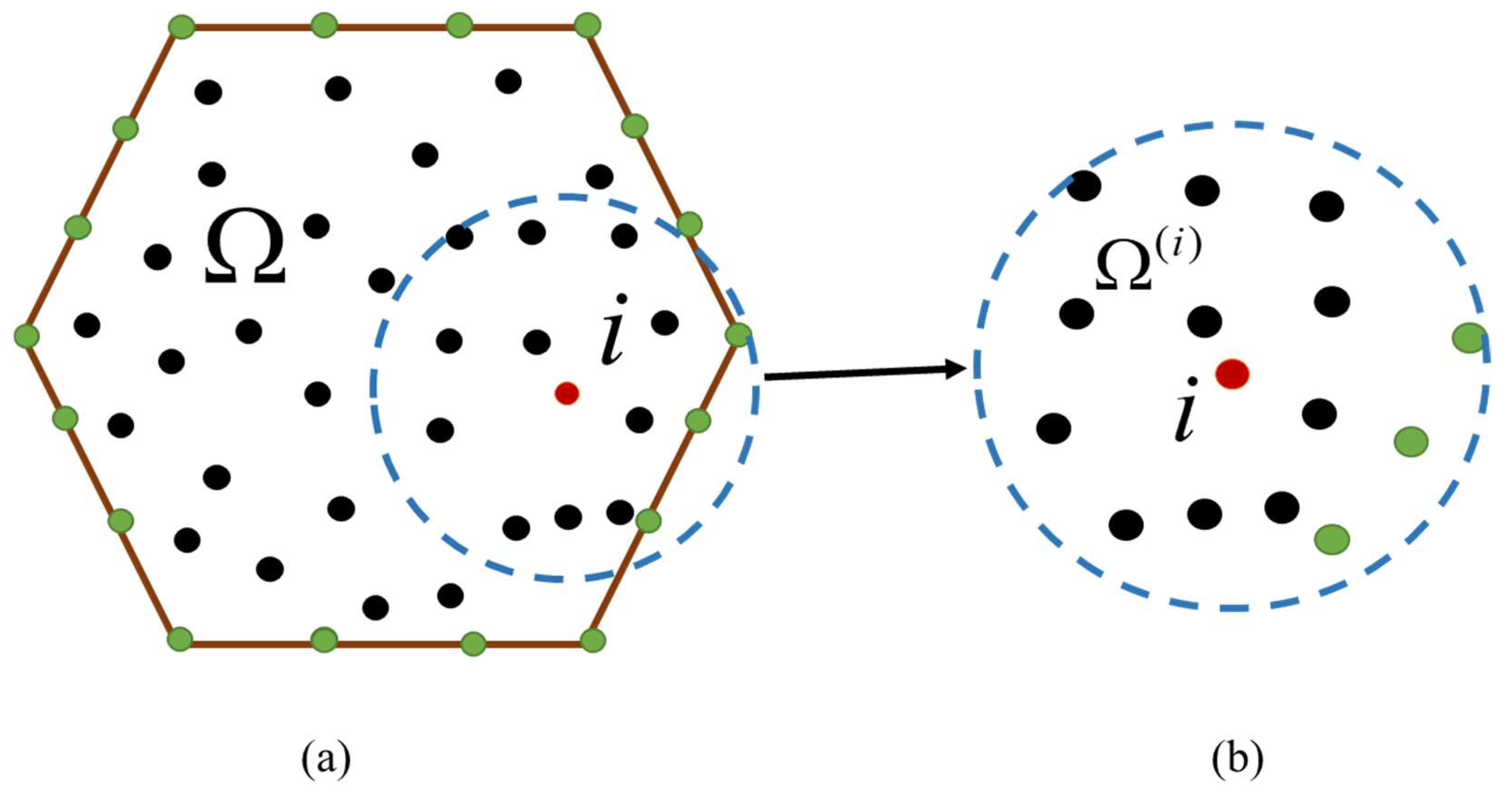
In this study, we used a localized BKM to solve this two-dimensional Cauchy inverse problem, whose governing equation is the Laplace equation. However, the traditional boundary knot method is extended from the method of the fundamental solution, and this study improves the global-type meshless method by changing it into the local type. $N=n_i+n_{b1}+n_{b2}$ is assumed to represent the total number of points to be calculated, where $n_i$ represents the number of internal points, while $n_{b1}$ and $n_{b2}$ represent the points of two kinds of boundary, i.e., ${\mathrm{\Gamma }}^D$ and ${\mathrm{\Gamma }}^N$, respectively. A schematic diagram of the calculation nodes of the localized BKM method is shown in Figure 1a.

In the localized BKM method, a subdomain is formed in each node, as shown in Figure 1b. The numerical solution for each subdomain can be approximately expressed as follows:

$$U(x_i,y_i)={\displaystyle \sum _{k=1}^{n_k}{\alpha }_k}G(r_k), x,y\in \mathrm{\Omega },$$

(6)

in which ${\alpha }_j$ stands for the unknown coefficients, and N is the number of adjacent nodes. $G(r_k)=e^{(-c(x^2-y^2))}\cos (2cxy)$ is the BKM basis function, which satisfies the two-dimensional Laplace equation. $n_k$ is the number of nodes in a subdomain. c is the shape parameter. $c=0.1$ is adopted in the following case. $r=\sqrt{x^2+y^2} (x=‖x-x_k‖, y=‖y-y_k‖)$ is the Euclidean distance, where $x_k$ and $y_k$ represent the x and y coordinates of the local node near the computing node, respectively. The source points are obtained from the nearest computing nodes in the subdomain.

By introducing the spatial coordinates of the nearest nodes into Equation (6), the following system is obtained:

$$U^{(i)}=C{\alpha }^{(i)},$$

(7)

where $U^{(i)}={[u_1^{(i)} u_2^{(i)} u_3^i \dots u_N^{(i)}]}^T$ is the vector of unknown variables at $n_k$ nodes, and ${\alpha }^{(i)}={[{\alpha }_1^{(i)} {\alpha }_2^{(i)} {\alpha }_3^{(i)} \dots {\alpha }_m^{(i)}]}^T$ is the vector of the unknown coefficients. C is the coefficient matrix. The unknown coefficients can be expressed by unknown variables:

$${\alpha }^{(i)}=C^{-1}{U}^{(i)}.$$

(8)

The inverse matrix $C^{-1}$ is calculated by using the MATLAB command pinv, and we set the tolerance to be 10⁻³–10⁻⁴ in this article.

The numerical solution for the ith node can be obtained from introducing the node coordinates of this point into Equation (7). The form is as follows:

$$U_{(i)}={\displaystyle \sum _{k=1}^{n_k}{\alpha }_k^{(i)}}G(r_k)=c^{(i)T}{\alpha }^{(i)}=c^{(i)T}{C}^{(-1)}{U}^{(i)}={\displaystyle \sum _{k=1}^{n_k}{\psi }_k^i}{U}_k^i,$$

(9)

where $c^{(i)}={[G(r_{i1}{) G(r}_{i2}) G(r_{i3}) \dots G(r_{i{n}_k})]}^T$ is the vector of the fundamental solution at the ith node. ${\{{\psi }_k^{(i)}\}}_{k=1}^{n_k}$ represents the weighting coefficients.

In addition, according to Equation (3), we have

$${\left.\frac{\partial U}{\partial x}\right|}_i={\left.{\displaystyle \sum _{k=1}^{n_k}{\alpha }_k^{(i)}}\frac{\partial }{\partial x}G(r_k)\right|}_i=h_x^{(i)T}{\alpha }^{(i)}=h_x^{(i)T}{H}^{-1}{U}^{(i)}={\displaystyle \sum _{k=1}^{n_k}{\psi }_k^{x(i)}}{U}_k^i,$$

(10)

and

$${\left.\frac{\partial U}{\partial y}\right|}_i={\left.{\displaystyle \sum _{k=1}^{n_k}{\alpha }_k^{(i)}}\frac{\partial }{\partial y}G(r_k)\right|}_i=h_y^{(i)T}{\alpha }^{(i)}=h_y^{(i)T}{H}^{-1}{U}^{(i)}={\displaystyle \sum _{k=1}^{n_k}{\psi }_k^{y(i)}}{U}_k^i,$$

(11)

where

$$h_x^{(i)}={\left[{\left.\frac{\partial G(r_1)}{\partial x}\right|}_i {\left.\frac{\partial G(r_2)}{\partial x}\right|}_i {\left.\frac{\partial G(r_3)}{\partial x}\right|}_i \dots {\left.\frac{\partial G(r_k)}{\partial x}\right|}_i\right]}^T,$$

(12)

$$h_y^{(i)}={\left[{\left.\frac{\partial G(r_1)}{\partial y}\right|}_i {\left.\frac{\partial G(r_2)}{\partial y}\right|}_i {\left.\frac{\partial G(r_3)}{\partial y}\right|}_i \dots {\left.\frac{\partial G(r_k)}{\partial y}\right|}_i\right]}^T$$

(13)

In order to obtain the expression for the Neumann boundary conditions, we can bring Equations (10) and (11) into Equation (3):

$$\frac{\partial U}{\partial n}=\frac{\partial U}{\partial x}{n}_x+\frac{\partial U}{\partial y}{n}_y=q(x,y), x,y\in {\mathrm{\Gamma }}^N$$

(14)

The linear equations that satisfy the Laplace equation, Dirichlet boundary conditions and Neumann boundary conditions are combined to form sparse linear algebraic equations,

$$AU=b,$$

(15)

where $A_{N\times N}$ is the sparse coefficient matrix that avoids the ill-conditioned matrix, $U={\left[U_1 U_2 U_3 \dots U_N\right]}^T$ is the unknown field quantity at every node and $b$ represents the known conditions. Therefore, $U$ can be calculated from Equation (15). The localized BKM, which combines BKM with the localization concept of localized MFS, is simple and clear, and the method of determining local points is also novel. In addition, due to the sparse matrix generated in the calculation of linear algebraic equations, it can also be applied to some complex fields.

4. Numerical Results and Comparisons

In this section, we present an analysis and comparison of the results of five cases. These five examples include a simply connected domain and a multi-connected domain. At the same time, different levels of noise are added to the boundary conditions to verify the stability of the localized BKM. For the last case, we carry out the process of forward calculation and then reverse calculation by guessing the analytical solution and relative error of the Laplace equation. In this paper, we compare the analytical solution $u_a$ with the numerical solution $U$ and take the maximum relative error as the index of error analysis.

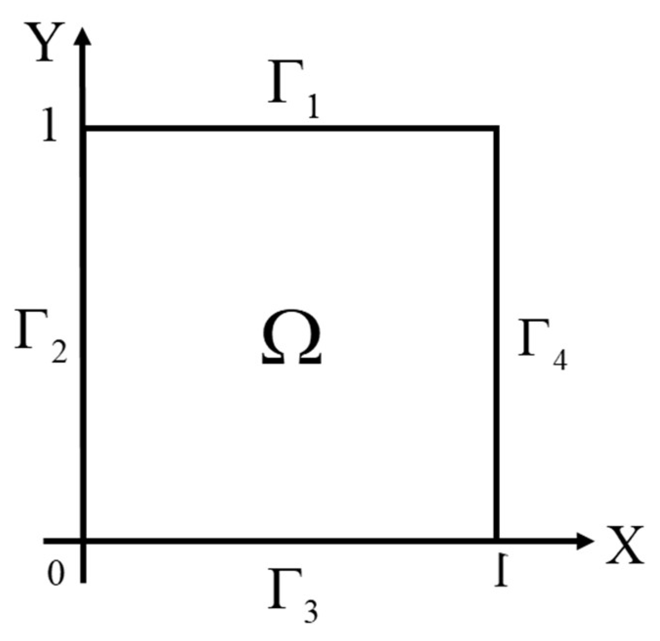
$$error=max(|(U-u_a)/u_a|).$$

4.1. Case 1

In the first example, we use a square computing field, as shown in Figure 2. The field is denoted by $\partial \mathrm{\Omega }={\mathrm{\Gamma }}_1+{\mathrm{\Gamma }}_2+{\mathrm{\Gamma }}_3+{\mathrm{\Gamma }}_4$. The boundary corner points are removed, and the internal points and boundary points are evenly distributed throughout the entire calculation domain. The analytical solution of the applied boundary condition is as follows:

$$u_a(x,y)=e^x\cos (y)+e^y\sin (x)+5,$$

(16)

where the ${\mathrm{\Gamma }}_1$ boundary is unknown, and the overdetermined boundary conditions (Dirichlet and Neumann) are added to the remaining edges, which are ${\mathrm{\Gamma }}_2, {\mathrm{\Gamma }}_3$ and ${\mathrm{\Gamma }}_4$. Hence, the points on this edge are calculated as interior points. The following parameters are used in this example: $N=4896, n_b=272, n_k=100, c=0.1$, where N is the number of total nodes, while $n_b$ is the number of boundary nodes.

In order to reflect the real boundary conditions, different levels of noise $s$ are added to the boundary to consider possible errors in advance. Therefore, the boundary conditions take the following forms:

$$u_a=f(x,y)(1+\frac{s}{100}\times rand), (x,y)\in {\mathrm{\Gamma }}_2+{\mathrm{\Gamma }}_3+{\mathrm{\Gamma }}_4,$$

(17)

$$\begin{array}{l}{u}_{an}=[(\nabla u)\cdot \overrightarrow{n}](1+\frac{s}{100}\times rand)=g(x,y)(1+\frac{s}{100}\times rand)\\ =[\nabla (u_a(x,y))\cdot \overrightarrow{n}](1+\frac{s}{100}\times rand), (x,y)\in {\mathrm{\Gamma }}_2+{\mathrm{\Gamma }}_3+{\mathrm{\Gamma }}_4\end{array}$$

(18)

where s is the percentage of added noise, rand is the random number and the range is $-1\le rand\le 1$. The function rand in MATLAB software is used in this paper to generate the noise.

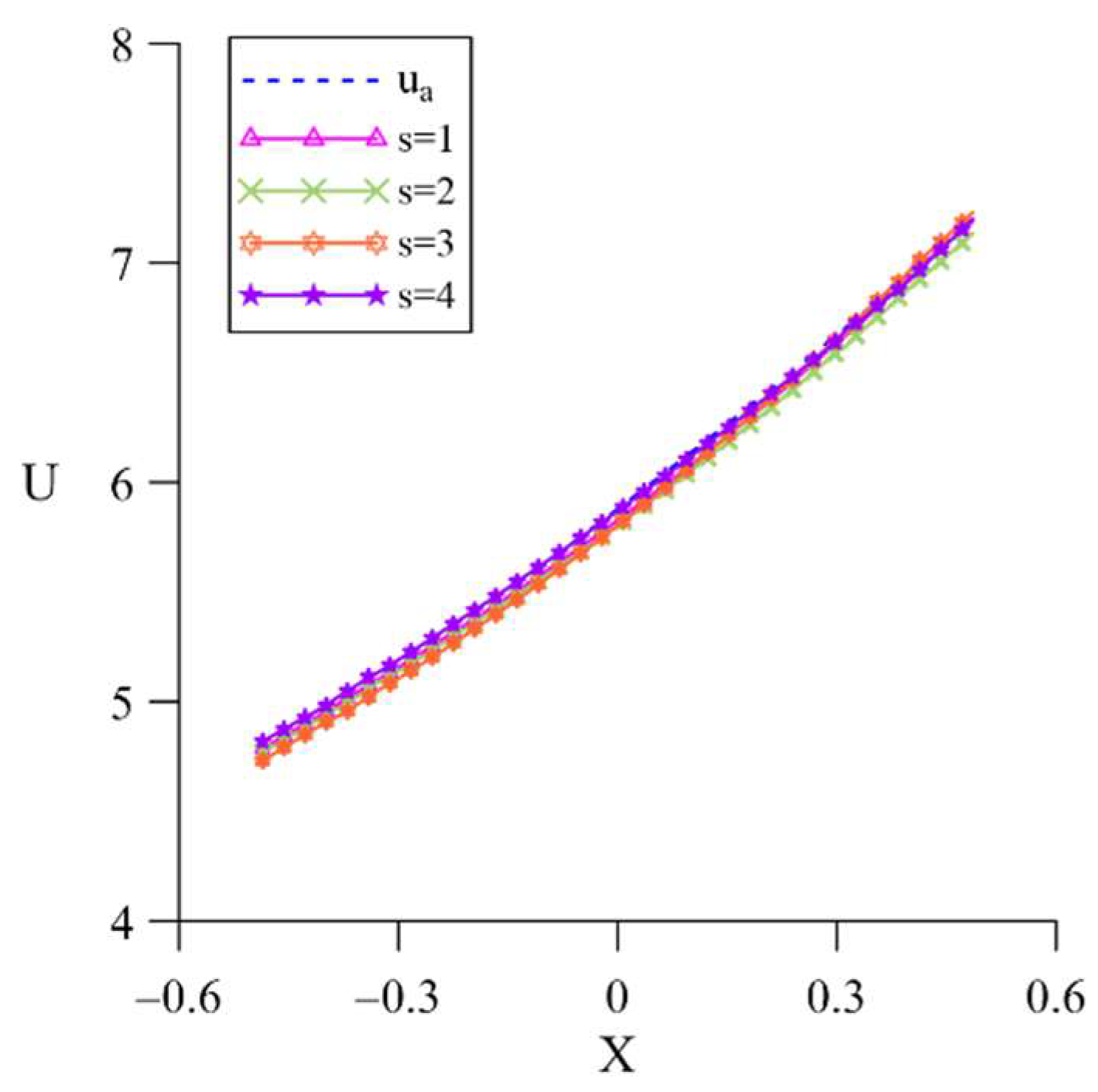
In order to show the calculation results more clearly, we draw the solution along the boundary ${\mathrm{\Gamma }}_1$, as shown in Figure 3. In this figure, we can see that, although different degrees of noise interference are added, the numerical solution along the boundary ${\mathrm{\Gamma }}_1$ is relatively stable, and the line-fitting degree with the analytical solution is relatively high.

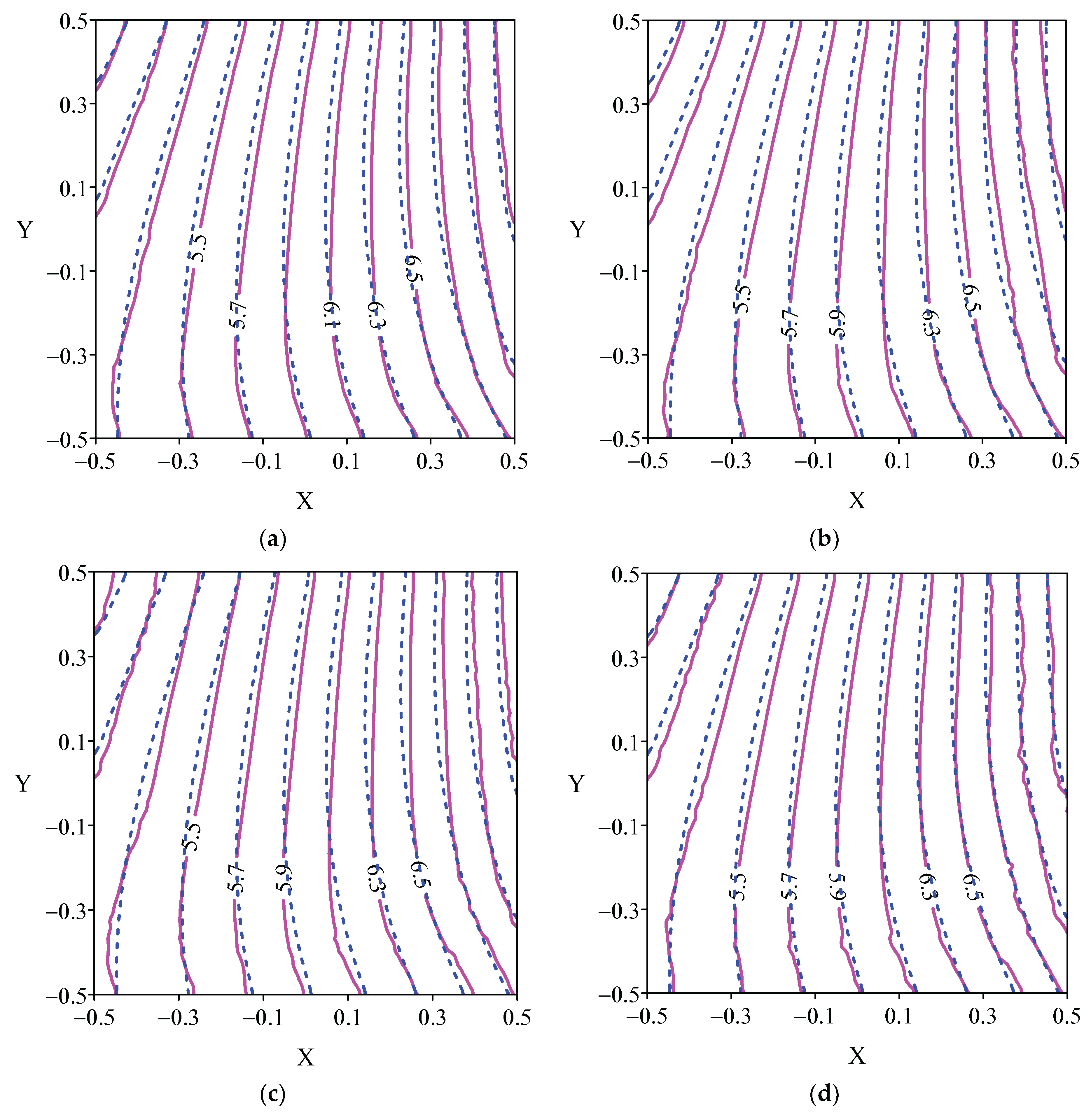
In Figure 4, we use a solid line to represent the internal numerical solution and a dotted line to represent the internal analytical solution. It can be seen from these four pictures that the errors increase with an increase in added noise, but they are all within the acceptable range, and those near the unknown boundary increase significantly. In

Table 1. The maximum relative error obtained by adding different percentages of noise for case 1.

Percentage of Noise	s = 1	s = 2	s = 3	s = 4	s = 5	s = 6	s = 7
Maximum relative error	0.00943	0.0136	0.0147	0.0184	0.0189	0.0209	0.0286

, we describe the maximum relative error corresponding to different degrees of disturbance in detail.

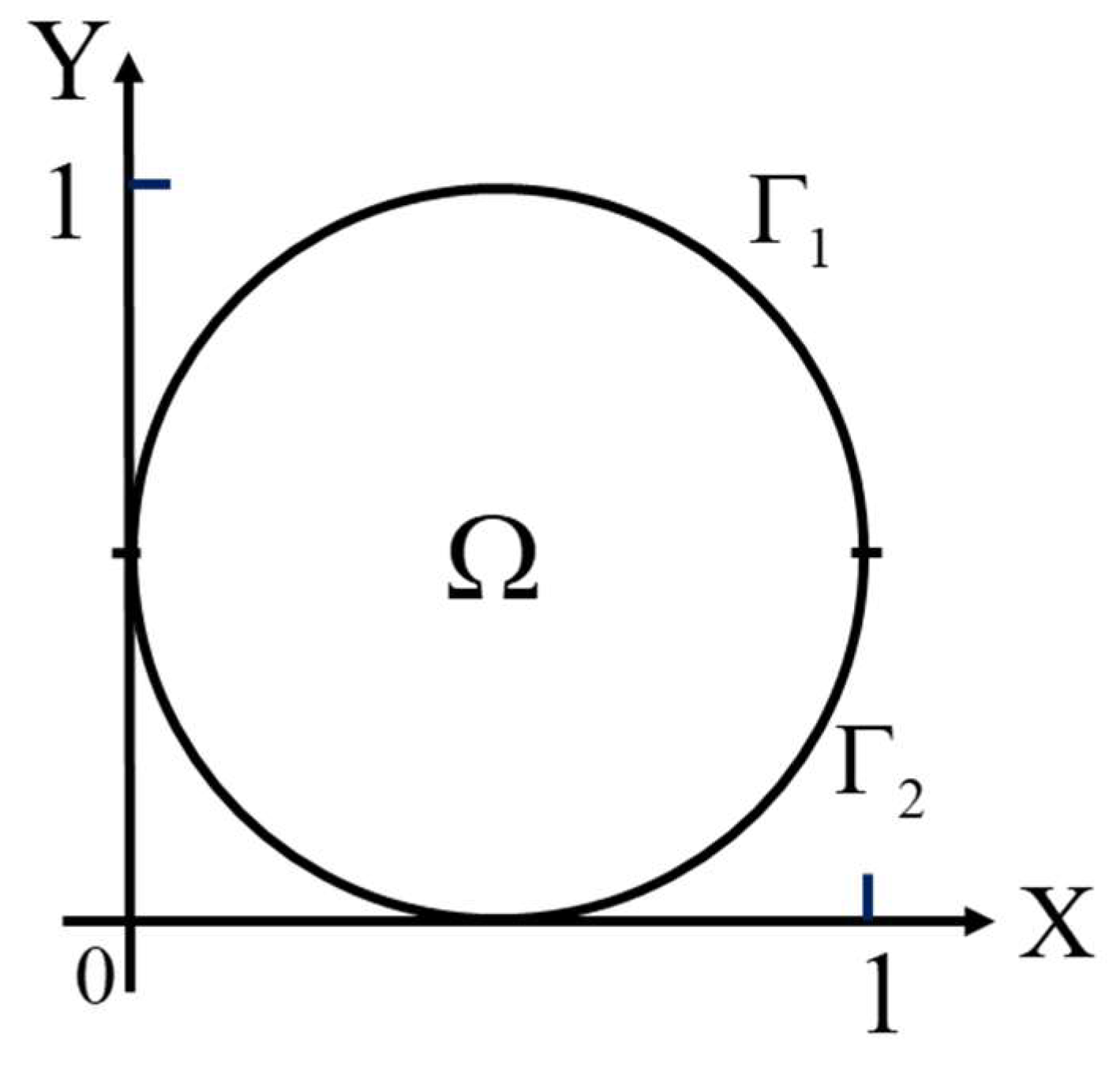
4.2. Case 2

In this case, a circle is used as the calculation domain, as shown in Figure 5. The radius of the circle is 1, and half of the boundary is unknown. ${\mathrm{\Gamma }}_1$ is an unknown boundary, while ${\mathrm{\Gamma }}_2$ is a known boundary. The analytical solution for this example is:

$$u_a=x^2-y^2+xy+5$$

(19)

The following parameters are used in this example: $N=2809, n_b=200,$$n_k=100, c=0.1$. The boundary conditions take the following forms:

$$\begin{array}{ll}u& =f(x,y)(1+\frac{s}{100}\times rand)\\ & =(x^2-y^2+xy+5)(1+\frac{s}{100}\times rand), (x,y)\in {\mathrm{\Gamma }}_2\end{array}$$

(20)

$$\begin{array}{ll}{u}_{an}& =[(\nabla u)\cdot \overrightarrow{n}](1+\frac{s}{100}\times rand)=g(x,y)(1+\frac{s}{100}\times rand)\\ & =[\nabla (x^2-y^2+xy+5)\cdot \overrightarrow{n}](1+\frac{s}{100}\times rand), (x,y)\in {\mathrm{\Gamma }}_2\end{array}$$

(21)

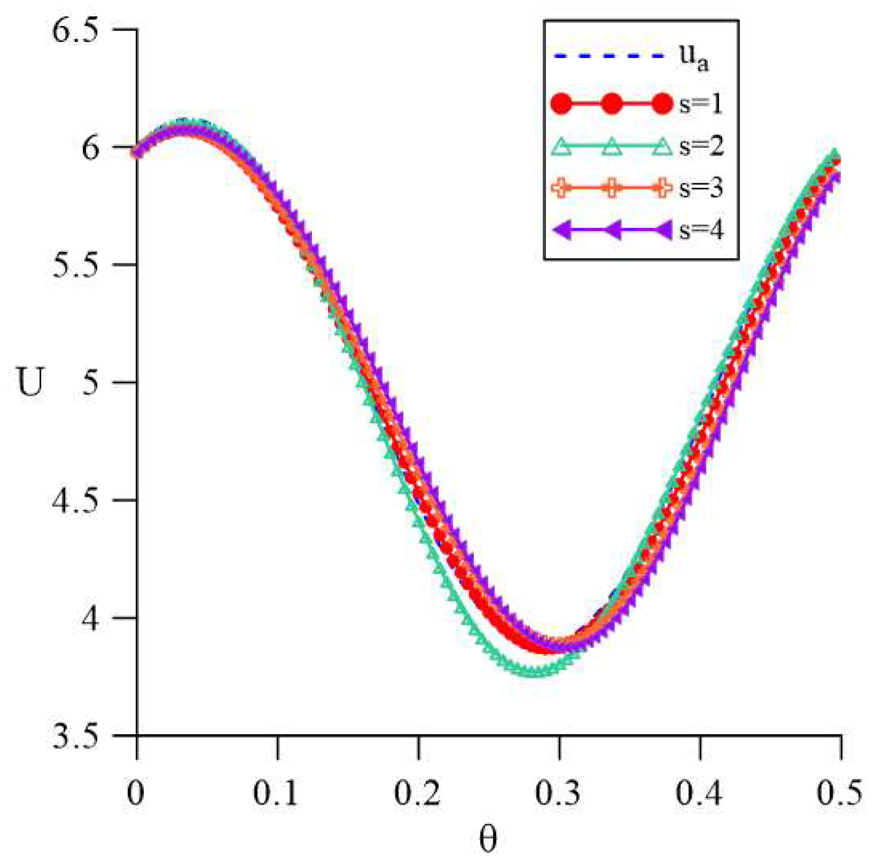
The marked solid lines in Figure 6 represent the numerical results for the unknown boundary ${\mathrm{\Gamma }}_1$ under different noise disturbances, and the dotted line represents the analytical solution curve of ${\mathrm{\Gamma }}_1$. Obviously, the numerical solutions are in good agreement with the analytical solution.

In

Table 2. The maximum relative error obtained by adding different percentages of noise for case 2.

Percentage of Noise	s = 1	s = 2	s = 3	s = 4	s = 5	s = 6	s = 7
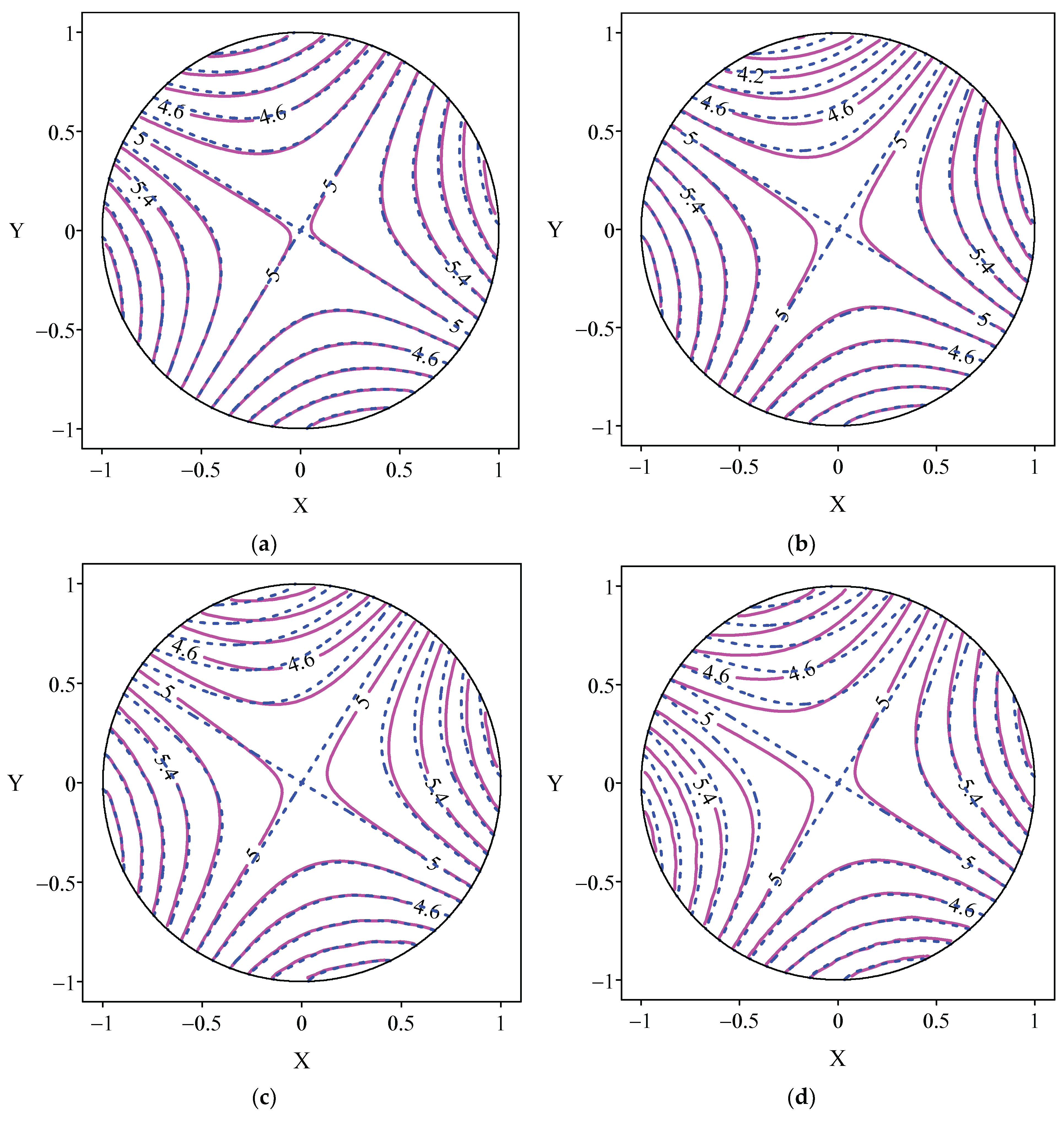
Maximum relative error	0.0198	0.0272	0.0347	0.0428	0.0504	0.0596	0.0779

, we list the maximum relative error obtained when adding different degrees of noise, and they are all very small. In Figure 7, we draw the internal distributions under different disturbances. The error near the unknown boundary is relatively large but is still within the acceptable range. The analytical solution line and the numerical solution line near the boundary with known boundary conditions fit well.

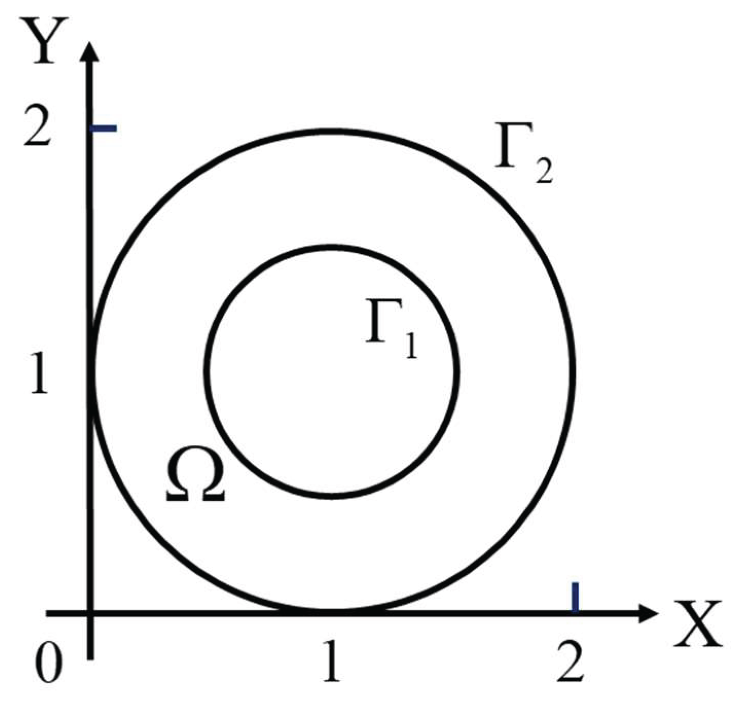
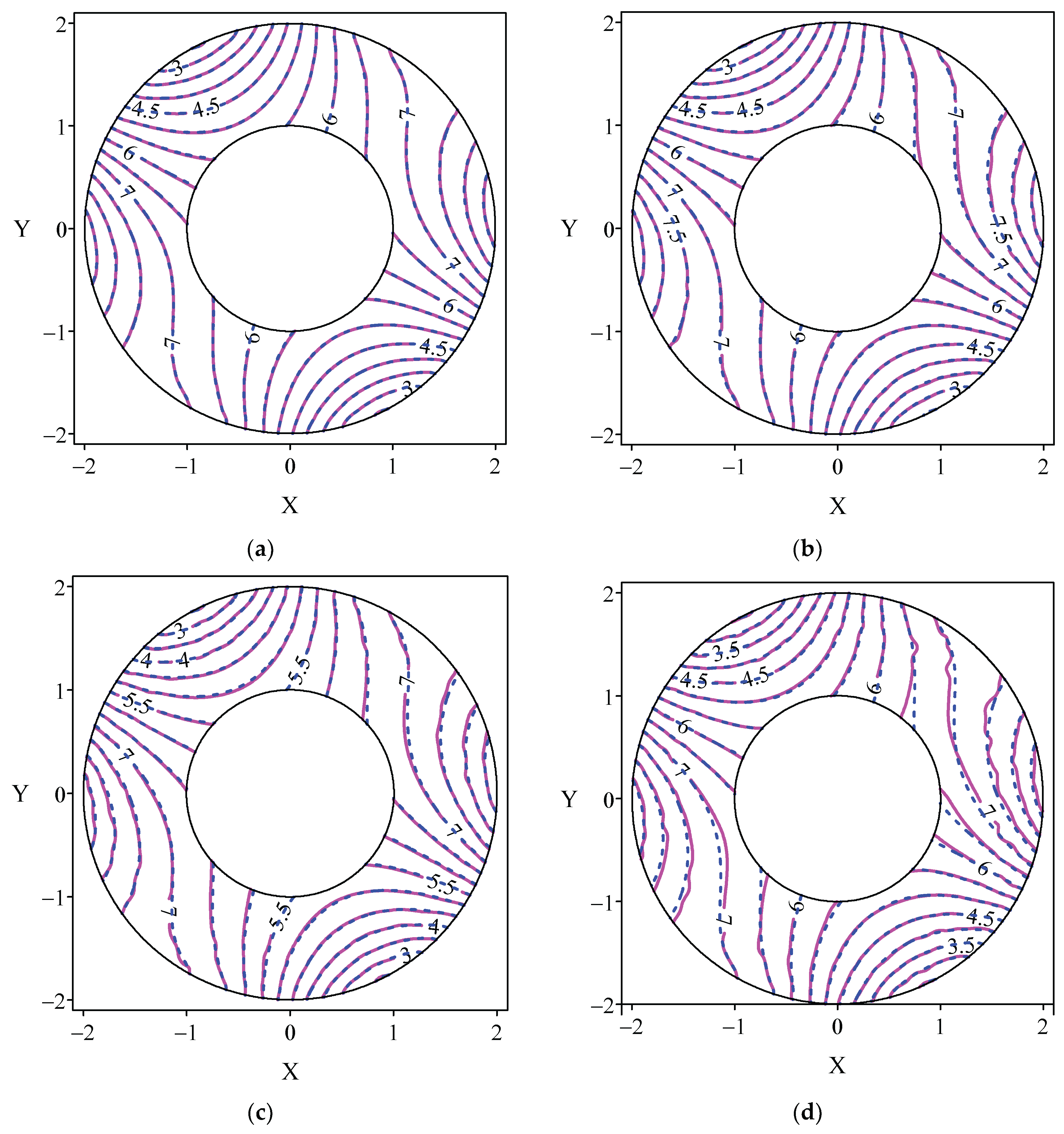
4.3. Case 3

For the third inverse problem, we use a doubly connected domain. The computational domain is concentric annular, as shown in Figure 8. The radius of the outer circle is 2, and the radius of the inner circle is 1. The analytical solution for this example is:

$$u_a=\sinh (y)\sin (x)+\cosh (x)\cos (y)+5.$$

(22)

The outer boundary has two kinds of boundary conditions, while the inner boundary has no boundary conditions. The given boundary conditions are obtained by the analytical solution, and the nodes are uniformly distributed in the computational domain and on the boundary. The parameters used in this example are as follows:

$N=1476, n_{b1}=380, n_{b2}=180, n_k=60, c=0.1$, where $n_{b1}$ and $n_{b2}$ represent the numbers of nodes on the outer and inner boundaries, respectively.

In

Table 3. The maximum relative error obtained by adding different percentages of noise for case 3.

Percentage of Noise	s = 0	s = 1	s = 2	s = 3	s = 4	s = 5	s = 6	s = 7
Maximum relative error	9.45 × 10−5	0.0056	0.0146	0.0214	0.0274	0.0375	0.0465	0.0654

, we list the maximum relative errors obtained when adding different degrees of noise, and the errors are also stable. A comparison of the analytical and numerical solutions drawn along the unknown boundary is shown in Figure 9. An internal contour map of different degrees of disturbance is shown in Figure 10. It can be seen from the figures that the numerical solution and the analytical solution are very similar.

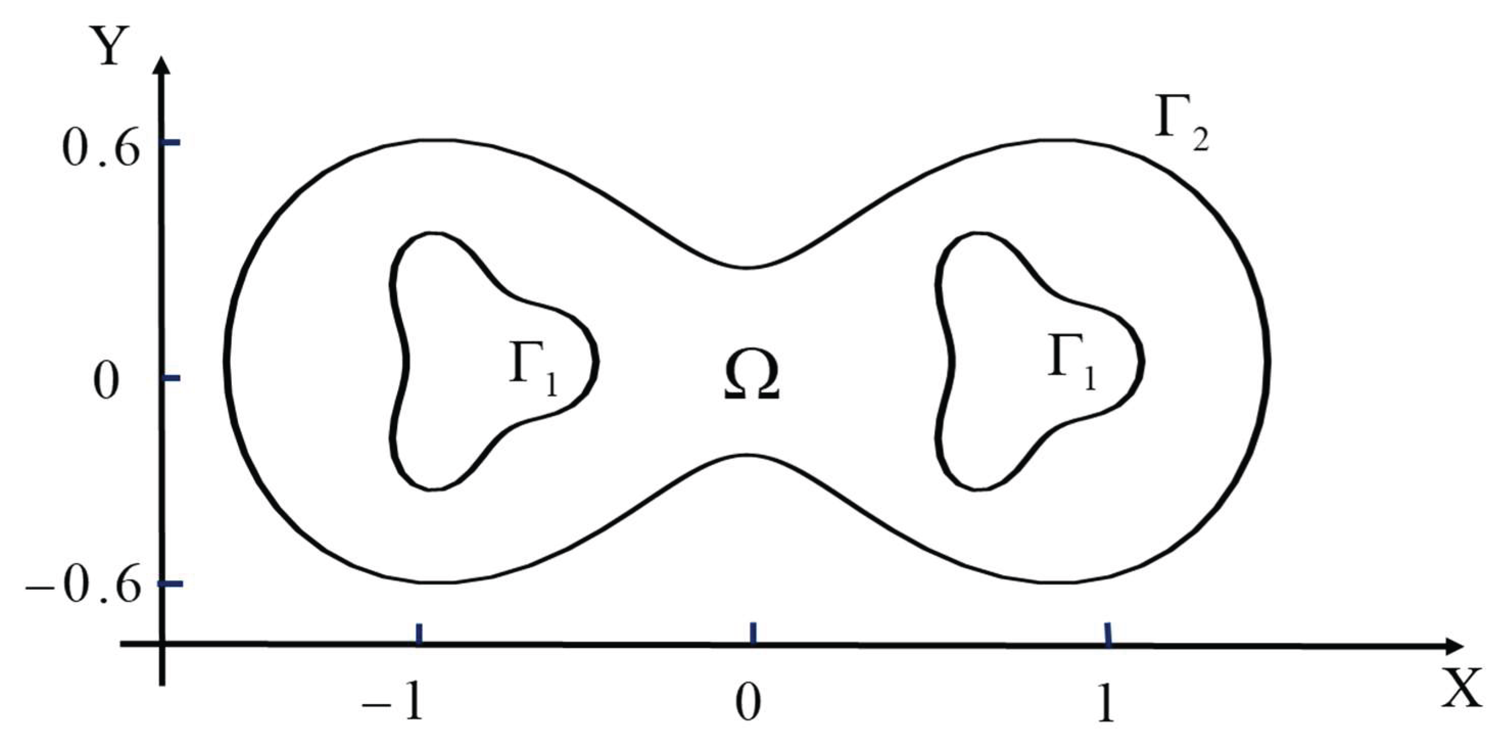
4.4. Case 4

In order to verify the stability of the numerical method, we use the multi-connected domain as the computational domain in this case, as shown in Figure 11. In this case, we take the outer boundary ${\mathrm{\Gamma }}_2$ as the unknown boundary and the inner boundary ${\mathrm{\Gamma }}_1$ as the known boundary. Therefore, two kinds of boundary conditions are added to the inner boundary. The analytical solution for this example is:

$$u_a=x^2-y^2+xy+5.$$

(23)

The boundary of the peanut shape is regarded as an unknown boundary, so the points on the boundary are calculated as internal nodes. Two internal wave elimination blocks are used as known boundaries, and a Dirichlet boundary condition and Neumann boundary condition are added. The parameters used in this example are as follows:

$$N=3068, n_{b1}=120, n_{b2}=102, n_k=100, c=0.1.$$

In

Table 4. The maximum relative error obtained by adding different noise for case 4.

Percentage of Noise	s = 0	s = 1	s = 2	s = 3	s = 4	s = 5	s = 6
Maximum relative error	1.96 × 10−4	0.0154	0.0196	0.0277	0.0496	0.0590	0.0688

, we list the maximum relative errors obtained when adding different degrees of noise, and the errors are also stable. A comparison of the analytical and numerical solutions drawn along the unknown boundary is shown in Figure 12. The data from tables and graphs show that the error is relatively stable and small.

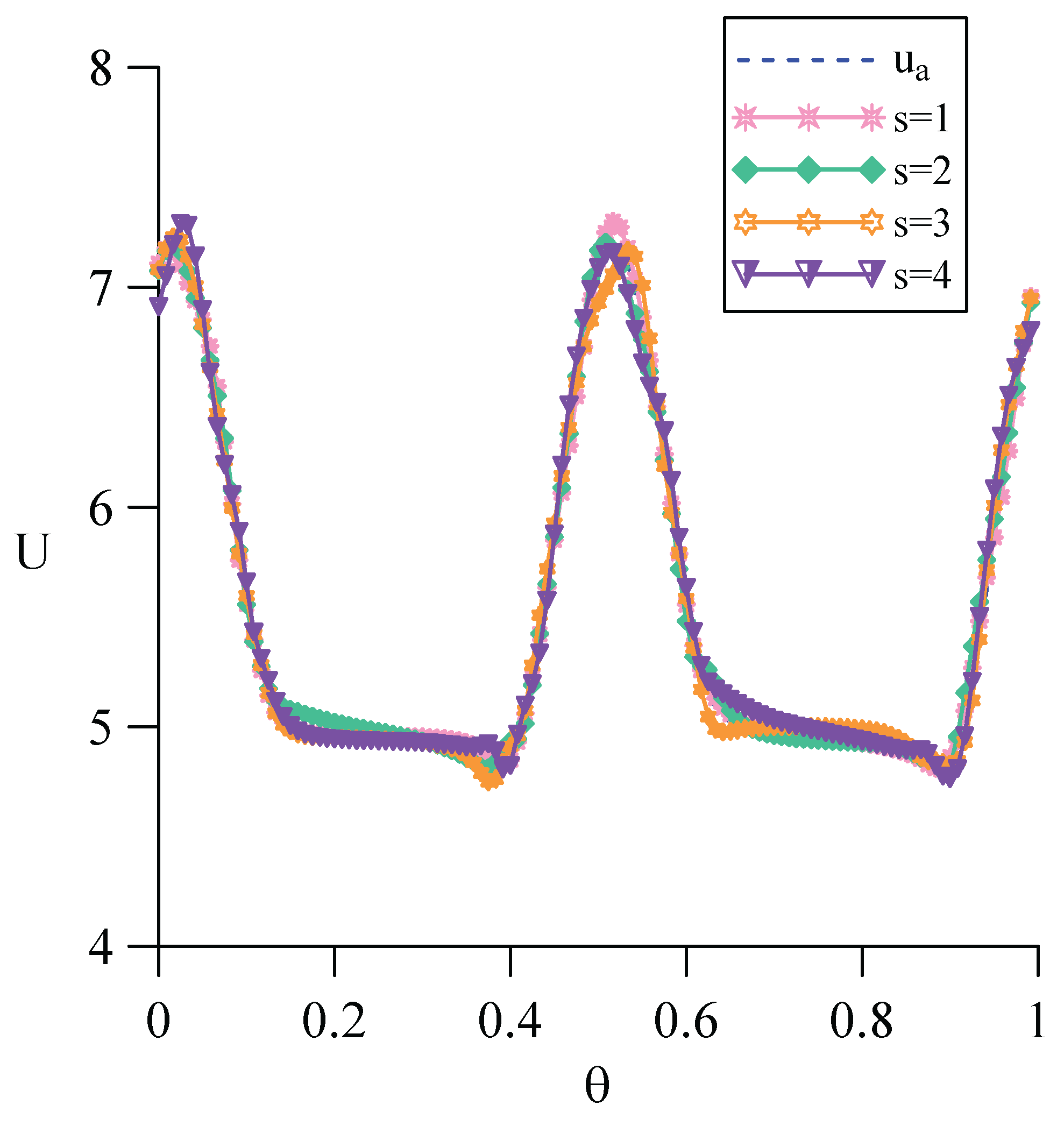
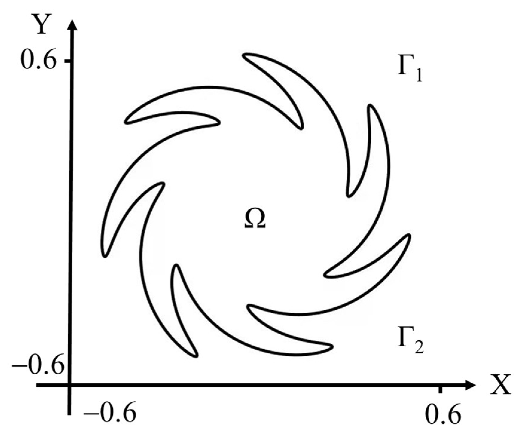
4.5. Case 5

In this example, the geometry of this computational domain is more complex and there are many sharp angles at the boundary; its schematic diagram is shown in Figure 13. The equation for the gear shape is as follows:

$$\partial \mathrm{\Omega }=\left\{\left(x,y\right)|x=\rho \left(\theta \right)\cos \left(\gamma \left(\theta \right)\right),y=\rho \left(\theta \right)\sin \left(\gamma \left(\theta \right)\right)\right\},$$

(24)

where $\rho \left(\theta \right)=0.2\left(2+0.5\sin \left(7\theta \right)\right), \gamma \left(\theta \right)=\theta +0.5\sin \left(\theta \right), 0\le \theta \le 2\pi$.

We set the boundary conditions ($0<\theta \le \pi$) of the upper half as unknown and the boundary conditions of the lower half ($\pi <\theta \le 2\pi$) as given. The Dirichlet boundary condition and the Neumann boundary condition are given by the following analytical solution:

$$u_a=\cos \left(x\right)\sinh \left(y\right)+x^2-y^2+xy+1$$

(25)

The following parameters are used: $N=901, n_{b1}=150, n_{b2}=150, n_k=80, c=0.1$.

From

Table 5. The maximum relative error obtained by adding different noise for case 5.

Percentage of Noise	s = 0	s = 1	s = 2	s = 3	s = 4	s = 5	s = 6
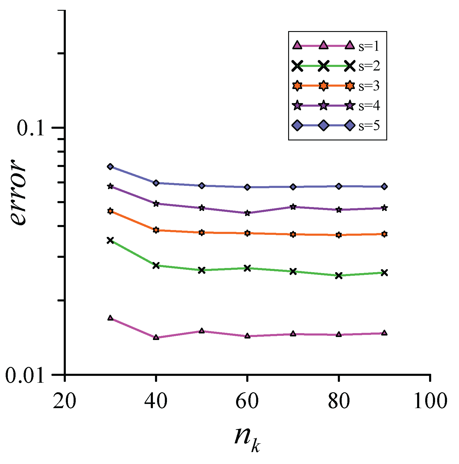
Maximum relative error	7.39 × 10−4	0.0150	0.0265	0.0376	0.0473	0.0582	0.0675

, it can be observed that even the geometry of the boundary is more complex under the setting of different levels of noise, and we can use the localized boundary knot method to solve this inverse Cauchy problem and still maintain a stable level of accuracy. Additionally, Figure 14 clearly shows the error curves obtained by applying different percentages of noise under different numbers of local points. This means that when the number of local points increases, the maximum relative error from the analytical solution approaches a stable state. 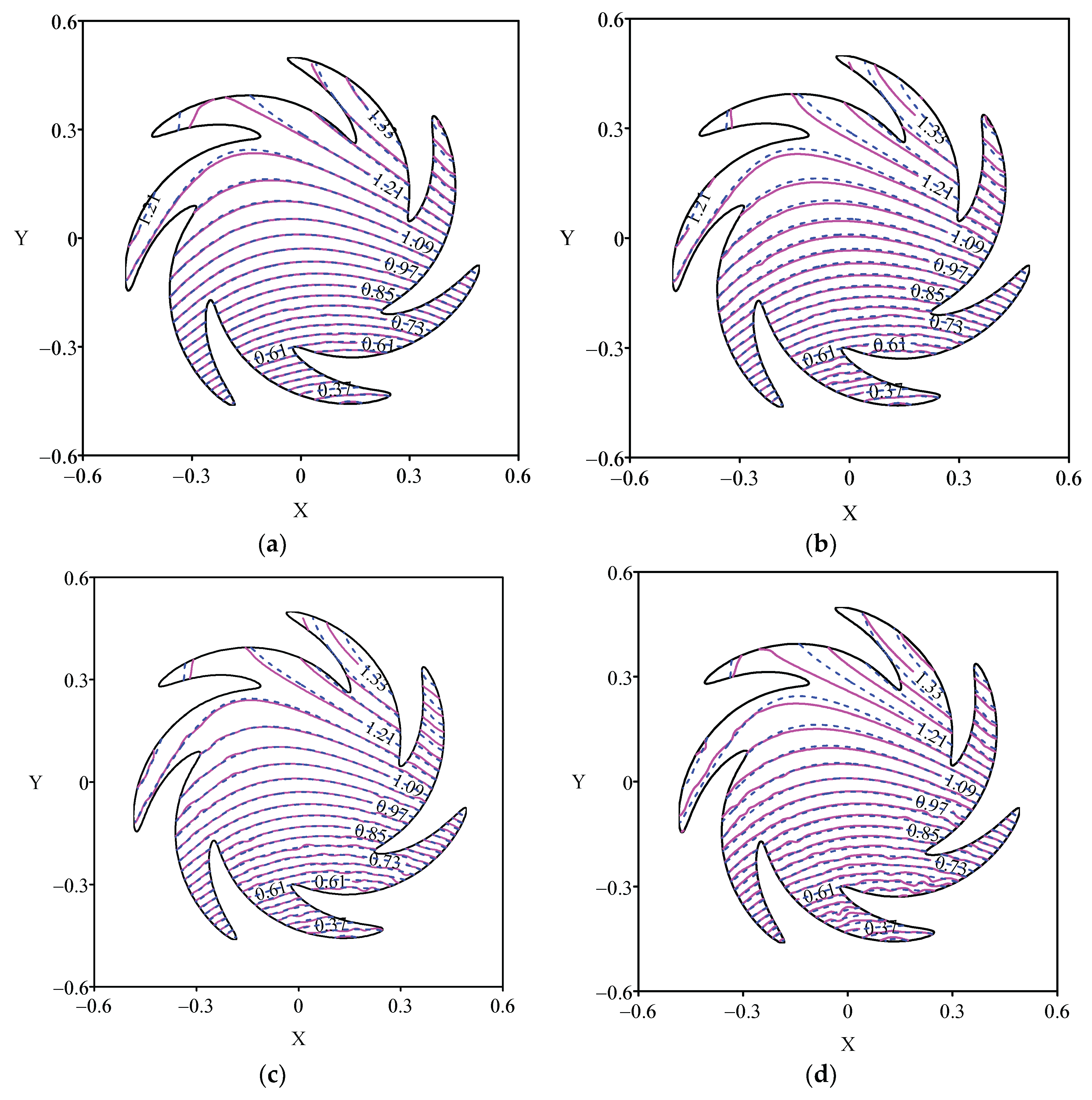In Figure 15, we show that (a) $s=1$, (b) $s=2$, (c) $s=3$ and (d) $s=4$. These four graphs show that there is indeed a certain degree of deviation in the upper half of the lack of boundary information, but the numerical results in the domain are consistent with the analytical solution.

4.6. Case 6

In order to further verify the accuracy of the localized BKM, in the last case, we also use the circle as the calculation domain, where a quarter of the boundary is used as the unknown boundary, namely ${\mathrm{\Gamma }}_2: \left(\frac{3}{2}\pi \le \theta \le 2\pi \right)$. We assume that the boundary conditions do not satisfy the analytical solution. This means that the corresponding analytical solution cannot be derived from the governing equations and boundary conditions. The known boundary satisfies the following conditions:

$$u=\left(\sinh (\frac{x}{4})+\cosh (\frac{x}{4})\right)\cos (\frac{y}{4})+50,x\in {\mathrm{\Gamma }}^D,$$

(26)

$$\frac{\partial u\left(x\right)}{\partial n}=\frac{1}{10}\left(x+y\right),x\in {\mathrm{\Gamma }}^N,$$

(27)

In Step 1, the boundary ${\mathrm{\Gamma }}_1: \left(0\le \theta <\frac{3}{2}\pi \right)$ is set as the Neumann boundary condition, and the boundary ${\mathrm{\Gamma }}_2$ is set as the Dirichlet boundary condition. The numerical solutions ${\left[u\right]}_{{\mathrm{\Gamma }}_1}$ can be solved by LBKM.

In Step 2, ${\mathrm{\Gamma }}_1$ is selected as the unknown boundary condition and the numerical solution obtained from the previous solution ${\left[u\right]}_{{\mathrm{\Gamma }}_1}$ and the Neumann boundary condition on the ${\mathrm{\Gamma }}_2$ boundary are used. For the first of the step calculation, the total number of nodes is $N=2949$, the number of boundary nodes is $n_b=200$, the number of local domain nodes is $n_k=100$, and the shape parameter is $c=0.1$, and for the second step of the calculation, the total number of nodes is $N=4249$, the number of boundary nodes is $n_b=200$, and the shape parameter is $c=0.1$. We analyze the maximum relative error of the numerical solutions for Step 1 and Step 2.

To show the stability of the numerical method, we solved this problem by using different numbers of local points, and the maximum relative error is presented in

Table 6. The maximum relative error obtained with different values of $n_k$ for case 6. ($N=2949$).

nk	40	70	100	130	150
Maximum relative error	3.75 × 10−3	7.22 × 10−4	1.20 × 10−3	1.92 × 10−3	1.72 × 10−3

. The change in maximum relative error corresponding to the change in total points is recorded in

Table 7. The maximum relative errors with different values of $N$ for case 6. ($n_k=100$).

N	3405	4093	5308	6380	8560
Maximum relative error	1.00 × 10−3	7.89 × 10−4	9.91 × 10−4	9.76 × 10−4	2.14 × 10−3

. It can be seen from the test of different total points $N$ and local points $n_k$ that, in the case where the boundary conditions do not use analytical solutions, the maximum relative error can still remain accurate and stable.

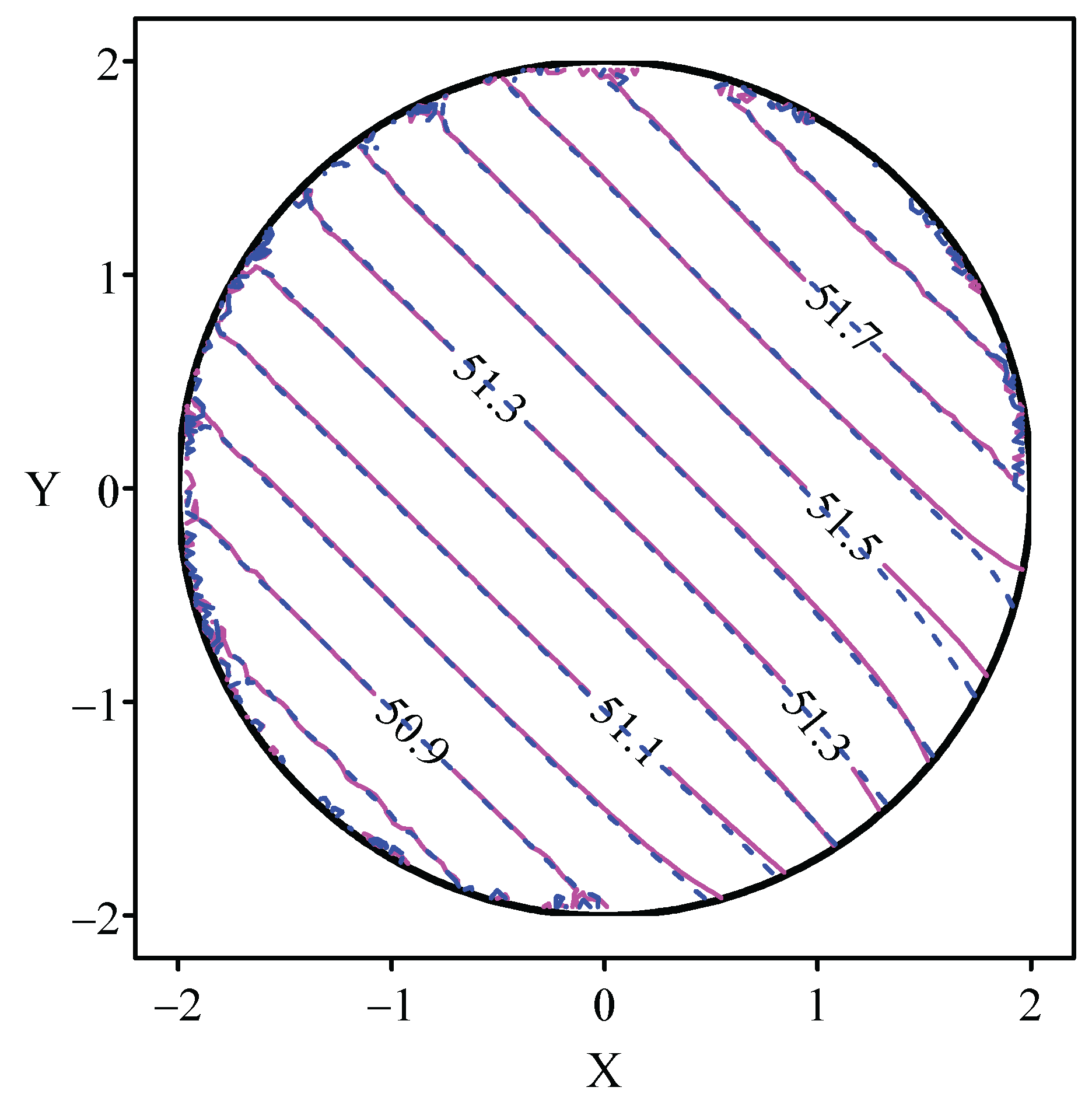
The distributions of numerical solutions to the direct and inverse problems are shown in Figure 16. In this figure, it can be seen that numerical solutions to the inverse problem are basically the same as in Step 1, and the maximum relative error is $7.89\times {10}^{-4}$.

5. Conclusions

In this paper, the localized BKM was used to solve an inverse Cauchy problem controlled by a two-dimensional Laplace equation. The localized BKM is a method that combines the BKM of the meshless method with the localization concept. This method does not need grid generation and numerical integration, and it eliminates border radius issues with source points. For Cauchy problems, some boundary conditions are not readily available or there are measurement errors, so the numerical simulation is unstable. Therefore, we used the localized BKM to calculate such problems and verify the accuracy of this method.

We presented five examples that illustrate the stability and accuracy of this method for solving inverse problems. With different percentages of noise on the boundaries, the maximum relative error remained stable and within the acceptable range. In particular, in the last case, the direct algorithm was first used to obtain the data with an extra boundary and was then applied to the reverse calculation in the second step. From the results of the error analysis presented in this paper, the localized BKM was shown to be more stable and accurate for solving Cauchy inverse problems.

In the future, the localized BKM will be applied to various mathematical and physical problems as well as more complex problems, for example, moving boundary problems and three-dimensional problems.

References

1. Chang, J.R.; Yeih, W.; Shieh, M.H. On the modified Tikhonov’s regularization method for the Cauchy problem of the Laplace equation. J. Mar. Sci. Technol. 2001, 9, 113–121. [Google Scholar] [CrossRef]
2. Chakib, A.; Nachaoui, A. Convergence analysis for finite element approximation to an inverse Cauchy problem. Inverse Probl. 2006, 22, 1191–1206. [Google Scholar] [CrossRef]
3. Vanrumste, B.; Van, H.G.; Van de Walle, R.; D’Havè, M.R.; Lemahieu, I.A.; Boon, P.A. The validation of the finite difference method and reciprocity for solving the inverse problem in EEG dipole source analysis. Brain Topogr. 2001, 14, 83–92. [Google Scholar] [CrossRef] [PubMed]
4. Lesnic, D.; Elliott, L.; Ingham, D.B. An iterative boundary element method for solving numerically the Cauchy problem for the Laplace equation. Eng. Anal. Bound. Elem. 1997, 20, 123–133. [Google Scholar] [CrossRef]
5. Mera, N.S.; Elliott, L.; Ingham, D.B.; Lesnic, D. An iterative boundary element method for the solution of a Cauchy steady state heat conduction problem. CMES Comput. Modeling Eng. Sci. 2000, 1, 101–106. [Google Scholar]
6. Lesnic, D.; Elliott, L.; Ingham, D.B. A alternating boundary element method for solving Cauchy problems for the biharmonic equation. Inverse Probl. Eng. 1997, 5, 145–168. [Google Scholar] [CrossRef]
7. Kansa, E.J. Multiquadrics—A scattered data approximation scheme with applications to computational fluid-dynamics—II solutions to parabolic, hyperbolic and elliptic partial differential equations. Comput. Math. Appl. 1990, 19, 147–161. [Google Scholar] [CrossRef] [Green Version]
8. Kansa, E.J. Multiquadrics—A scattered data approximation scheme with applications to computational fluid-Dynamics—I surface approximations and partial derivative estimates. Comput. Math. Appl. 1990, 19, 127–145. [Google Scholar] [CrossRef] [Green Version]
9. Hardy, R.L. Multiquadric equations of topography and other irregular surfaces. J. Geophys. Res. 1971, 76, 1905–1915. [Google Scholar] [CrossRef]
10. Duchon, J. Splines minimizing rotation-invariant semi-norms in Sobolev spaces. In Constructive Theory of Functions of Several Variables; Springer: Berlin/Heidelberg, Germany, 1977; pp. 85–100. [Google Scholar]
11. Franke, R. Scattered data interpolation: Tests of some methods. Math. Comput. 1982, 38, 181–200. [Google Scholar]
12. Nam, M.D.; Thanh, T.C. Mesh-free radial basis function network methods with domain decomposition for approximation of functions and numerical solution of Poisson’s equations. Eng. Anal. Bound. Elem. 2002, 26, 133–156. [Google Scholar]
13. Fan, C.M.; Huang, Y.K.; Li, P.W.; Chiu, C.L. Application of the generalized finite-difference method to inverse biharmonic boundary-value problems. Numer. Heat Transf. Part B Fundam. 2014, 65, 129–154. [Google Scholar] [CrossRef]
14. Fan, C.M.; Li, P.W.; Yeih, W. Generalized finite difference method for solving two-dimensional inverse Cauchy problems. Inverse Probl. Sci. Eng. 2015, 23, 737–759. [Google Scholar] [CrossRef]
15. Li, P.W.; Fan, C.M.; Grabski, J.K. A meshless generalized finite difference method for solving shallow water equations with the flux limiter technique. Eng. Anal. Bound. Elem. 2021, 131, 159–173. [Google Scholar] [CrossRef]
16. Li, P.W. Space–time generalized finite difference nonlinear model for solving unsteady Burgers’ equations. Appl. Math. Lett. 2021, 114, 106896. [Google Scholar] [CrossRef]
17. Chu, H.F.; Fan, C.M.; Yeih, W.C. Solution of inverse boundary optimization problem by Trefftz method and exponentially convergent scalar homotopy algorithm. CMC-Comput. Mater. Contin. 2011, 24, 125–142. [Google Scholar]
18. Liu, C.S.; Atluri, S.N. Numerical solution of the Laplacian Cauchy problem by using a better postconditioning collocation Trefftz method. Eng. Anal. Bound. Elem. 2013, 37, 74–83. [Google Scholar] [CrossRef]
19. Kołodziej, J.A.; Grabski, J.K. Many names of the Trefftz method. Eng. Anal. Bound. Elem. 2018, 96, 169–178. [Google Scholar] [CrossRef]
20. Liu, C.S. A highly accurate MCTM for direct and inverse problems of biharmonic equation in arbitrary plane domains. CMES: Comput. Modeling Eng. Sci. 2008, 30, 65–75. [Google Scholar]
21. Fan, C.M.; Chan, H.F. Modified collocation Trefftz method for the geometry boundary identification problem of heat conduction. Numer. Heat Transf. Part B Fundam. 2011, 59, 58–75. [Google Scholar] [CrossRef]
22. Gu, Y.; Chen, W.; Zhang, C.; He, X. A meshless singular boundary method for three-dimensional inverse heat conduction problems in general anisotropic media. Int. J. Heat Mass Transf. 2015, 84, 91–102. [Google Scholar] [CrossRef]
23. Fu, Z.; Chen, W.; Zhang, C. Boundary particle method for Cauchy inhomogeneous potential problems. Inverse Probl. Sci. Eng. 2012, 20, 189–207. [Google Scholar] [CrossRef]
24. Kupradze, V.D.; Aleksidze, M.A. The method of functional equations for the approximate solution of certain boundary value problems. USSR Comput. Math. Math. Phys. 1964, 4, 82–126. [Google Scholar] [CrossRef]
25. Karageorghis, A.; Lesnic, D. Detection of cavities using the method of fundamental solutions. Inverse Probl. Sci. Eng. 2009, 17, 803–820. [Google Scholar] [CrossRef]
26. Karageorghis, A.; Lesnic, D.; Marin, L. A survey of applications of the MFS to inverse problems. Inverse Probl. Sci. Eng. 2011, 19, 309–336. [Google Scholar] [CrossRef]
27. Young, D.L.; Tsai, C.C.; Chen, C.W.; Fan, C.M. The method of fundamental solutions and condition number analysis for inverse problems of Laplace equation. Comput. Math. Appl. 2008, 55, 1189–1200. [Google Scholar] [CrossRef] [Green Version]
28. Fan, C.M.; Li, P.W. Numerical solutions of direct and inverse stokes problems by the method of fundamental solutions and the Laplacian decomposition. Numer. Heat Transf. Part B Fundam. 2015, 68, 204–223. [Google Scholar] [CrossRef]
29. Chen, W.; Tanaka, M. A meshless, integration-free, and boundary-only RBF technique. Comput. Math. Appl. 2002, 43, 379–391. [Google Scholar] [CrossRef] [Green Version]
30. Chen, W. Symmetric boundary knot method. Eng. Anal. Bound. Elem. 2002, 26, 489–494. [Google Scholar] [CrossRef] [Green Version]
31. Jiang, X.; Chen, W.; Chen, C.S. Fast multipole accelerated boundary knot method for inhomogeneous Helmholtz problems. Eng. Anal. Bound. Elem. 2013, 37, 1239–1243. [Google Scholar] [CrossRef]
32. Chen, W.; Shen, L.J.; Shen, Z.J.; Yuan, G.W. Boundary knot method for Poisson equations. Eng. Anal. Bound. Elem. 2005, 29, 756–760. [Google Scholar] [CrossRef]
33. Jin, B.; Zheng, Y. Boundary knot method for some inverse problems associated with the Helmholtz equation. Int. J. Numer. Methods Eng. 2005, 62, 1636–1651. [Google Scholar] [CrossRef]
34. Jin, B.; Zheng, Y. Boundary knot method for the Cauchy problem associated with the inhomogeneous Helmholtz equation. Eng. Anal. Bound. Elem. 2005, 29, 925–935. [Google Scholar] [CrossRef]
35. Zheng, H.; Zhang, C.; Wang, Y.; Sladek, J.; Sladek, V. A meshfree local RBF collocation method for anti-plane transverse elastic wave propagation analysis in 2D phononic crystals. J. Comput. Phys. 2016, 305, 997–1014. [Google Scholar] [CrossRef]
36. Zheng, H.; Yao, G.; Kuo, L.H.; Li, X. On the selection of a good shape parameter of the localized method of approximated particular solutions. Adv. Appl. Math. Mech. 2018, 10, 896–911. [Google Scholar] [CrossRef]
37. Zheng, H.; Yang, Z.; Zhang, C.; Tyrer, M. A local radial basis function collocation method for band structure computation of phononic crystals with scatterers of arbitrary geometry. Appl. Math. Model. 2018, 60, 447–459. [Google Scholar] [CrossRef]
38. Zheng, H.; Xiong, J.G.; Yuan, Y.; Wen, P.H. Mixed-mode dynamic stress intensity factors by variation technique with finite block method. Eng. Anal. Bound. Elem. 2019, 106, 27–33. [Google Scholar] [CrossRef]
39. Chan, H.F.; Fan, C.M. The local radial basis function collocation method for solving two-dimensional inverse Cauchy problems. Numer. Heat Transf. Part B Fundam. 2013, 63, 284–303. [Google Scholar] [CrossRef]
40. Fan, C.M.; Huang, Y.K.; Chen, C.S.; Kuo, S. Localized method of fundamental solutions for solving two-dimensional Laplace and biharmonic equations. Eng. Anal. Bound. Elem. 2019, 101, 188–197. [Google Scholar] [CrossRef]
41. Wang, F.; Fan, C.M.; Hua, Q.; Gu, Y. Localized MFS for the inverse Cauchy problems of two-dimensional Laplace and biharmonic equations. Appl. Math. Comput. 2020, 364, 124658. [Google Scholar] [CrossRef]
42. Liu, Y.C.; Fan, C.M.; Yeih, W.; Ku, C.Y.; Chu, C.L. Numerical solutions of two-dimensional Laplace and biharmonic equations by the localized Trefftz method. Comput. Math. Appl. 2021, 88, 120–134. [Google Scholar] [CrossRef]
43. Wang, F.; Chen, Z.; Li, P.W.; Fan, C.M. Localized singular boundary method for solving Laplace and Helmholtz equations in arbitrary 2D domains. Eng. Anal. Bound. Elem. 2021, 129, 82–92. [Google Scholar] [CrossRef]
44. Wang, F.; Gu, Y.; Qu, W.; Zhang, C. Localized boundary knot method and its application to large-scale acoustic problems. Comput. Methods Appl. Mech. Eng. 2020, 361, 112729. [Google Scholar] [CrossRef]
45. Xiong, J.; Wen, J.; Liu, Y.C. Localized boundary knot method for solving two-dimensional Laplace and Bi-Harmonic equations. Mathematics 2020, 8, 1218. [Google Scholar] [CrossRef]
Figure 1. Schematic diagram of the localized boundary knot method. (a) The global domain. (b) The local domain of the ith node.
Mathematics 10 01324 g001
Figure 2. Schematic diagram for case 1.
Mathematics 10 01324 g002
Figure 3. The profiles of numerical solutions along Γ 1 for case 1.
Mathematics 10 01324 g003
Figure 4. The distributions of numerical (solid lines) and analytical solutions (dashed lines) (a) s = 1 (b) s = 2 (c) s = 3 (d) s = 4.
Mathematics 10 01324 g004
Figure 5. Schematic diagram for case 2.
Mathematics 10 01324 g005
Figure 6. The profiles of numerical solutions along Γ 1 for case 2.
Mathematics 10 01324 g006
Figure 7. The distributions of numerical (solid lines) and analytical solutions (dashed lines). (a) s = 1 (b) s = 2 (c) s = 3 (d) s = 4.
Mathematics 10 01324 g007
Figure 8. Schematic diagram for case 3.
Mathematics 10 01324 g008
Figure 9. The profiles of numerical solutions along Γ 1 for case 3.
Mathematics 10 01324 g009
Figure 10. The distributions of numerical (solid lines) and analytical solutions (dashed lines). (a) s = 1 (b) s = 2 (c) s = 3 (d) s = 4.
Mathematics 10 01324 g010
Figure 11. Schematic diagram for case 4.
Mathematics 10 01324 g011
Figure 12. The profiles of numerical solutions along Γ 2 for case 4.
Mathematics 10 01324 g012
Figure 13. Schematic diagram for case 5.
Mathematics 10 01324 g013
Figure 14. The maximum relative error of the different percentages of noise and local nodes for case 5.
Mathematics 10 01324 g014
Figure 15. The distributions of numerical (solid lines) and analytical solutions (dashed lines) for Case 6. (a) s = 1 (b) s = 2 (c) s = 3 (d) s = 4.
Mathematics 10 01324 g015
Figure 16. The numerical solution distribution of Step 1 (dashed lines) and Step 2 (solid lines) for case 6. ( N = 4093 ,   n k = 100 ).
Mathematics 10 01324 g016