Bayesian Influence Analysis of the Skew-Normal Spatial Autoregression Models

Abstract

In spatial data analysis, outliers or influential observations have a considerable influence on statistical inference. This paper develops Bayesian influence analysis, including the local influence approach and case influence measures in skew-normal spatial autoregression models (SSARMs). The Bayesian local influence method is proposed to evaluate the impact of small perturbations in data, the distribution of sampling and prior. To measure the extent of different perturbations in SSARMs, the Bayes factor, the $\varphi$-divergence and the posterior mean distance are established. A Bayesian case influence measure is presented to examine the influence points in SSARMs. The potential influence points in the models are identified by Cook’s posterior mean distance and Cook’s posterior mode distance $\varphi$-divergence. The Bayesian influence analysis formulation of spatial data is given. Simulation studies and examples verify the effectiveness of the presented methodologies.

1. Introduction

In the fields of econometrics, air quality monitoring and epidemic monitoring, spatial data are often encountered. Spatial data are a kind of data with location attributes, which usually have spatial dependence. If the spatial correlation of data is not considered, the conclusion will often be inaccurate or even wrong. Spatial autoregressive models (SARMs) can effectively deal with the data with spatial correlation [1]. Therefore, SARMs have attracted the extensive attention of many scholars over the past few years. For example, Piribauer and Cuaresma [2] proposed two Bayesian variable selection approaches and compared their performance in SARMs. Xie et al. [3] investigated the variable selection problem in SARMs; Du et al. [4] studied the generalized method of moments estimator for partially linear additive SARMs; Li et al. [5] considered a variable selection method for SARMs based on the minimum prediction error criterion; Jay et al. [6] introduced SARMs for the statistical inference of ecological data, which discussed model selection, spatial regression, the estimation of autocorrelation, the estimation of other connectivity parameters, spatial prediction and the spatial smoothing of practical ecological inference; Anik et al. [7] investigated a Lagrange multiplier test of spatial dependence for SARMs with latent variables; Song et al. [8] proposed a class of penalized robust regression estimators based on exponential squared loss for SARMs with independent identically distributed errors. The above studies of SSARMs are mainly based on the hypothesis that the dependent variable follows a normal distribution. However, the normal hypothesis is often excessively restrictive of the variability of spatial data in the actual statistical inference, and unreasonable results may be generated.

In the actual spatial data, there are few cases of strict symmetry. At this time, if the spatial data is studied based on the assumption of normality, it is difficult to capture the changes in the data. In recent years, the skew-normal distribution has attracted widespread attention. A large number of studies on skew-normal distribution have appeared under various statistical models. For example, Marcos et al. [9] developed nonlinear mixed-effects models for a mixture of scales with a skew-normal distributions family and gained an estimate of the parameters by the maximum likelihood method; Yin et al. [10] introduced a variable selection procedure for a finite mixture of regression models using the skew-normal distribution; Tatsuya et al. [11] investigated the decision–theoretic properties of Stein-type shrinkage estimators in multivariate skew-normal distribution under the condition of quadratic loss; Liu et al. [12] considered an autoregressive model based on the skew-normal distribution; Mahdi [13] adopted the EM algorithm to research the maximum likelihood estimation of the mixed model with a skewed-normal assumption. However, as far as we know, there are few studies on SARMs with the response variables following skew-normal distribution.

In recent years, the Bayesian methods of local influence and case influence analysis have become widely used statistical diagnostic methods. For Bayesian local influence analysis, it is extensively studied within different models based on several objective functions. For example, Zhu et al. [14] established a universal framework of Bayesian influence analysis to evaluate the impact of simultaneous perturbations of prior, data and sample distribution for a set of statistical models; Zhang et al. [15] proposed Bayesian local influence analysis to evaluate the impact of different perturbations of individual observations, prior distribution and nonignorable missing data mechanisms in general EEs. Ouyang et al. [16] applied the Bayesian local influence method to semiparametric structural equation models and the effects of minor perturbations were evaluated using different perturbation options; Dai et al. [17] studied two Bayesian local diagnostic procedures for heteroscedastic SARMs; Ju et al. [18] developed a new SDPDMs by assuming that the random effects and error terms obey a skew-normal distribution and also developed a Bayesian local influence analysis method for it. For Bayesian case influence diagnostics, they are widely researched in various statistical models based on conditional predictive coordinates and K-L distance. Cancho et al. [19] presented Bayesian case deletion influence diagnostics for nonlinear regression models with scale mixtures of skew-normal distributions based on the K-L divergence; Zhu et al. [20] proposed three Bayesian case influence measures to identify influential points for a class of statistical models with missing data, which included the Cook’s posterior mean and mode distance and $\varphi$-divergence; Tang et al. [21] detected the influence observations of generalized partial linear mixed models for longitudinal data based on $\varphi$-divergence and Cook’s posterior mean distance; Hao et al. [22] investigated Bayesian case influence analysis based on the K-L divergence of a generalized autoregressive conditional heteroscedasticity model; Duan et al. [23] developed a Bayesian case deletion influence measure based on the $\varphi$-divergence of a semiparametric reproductive dispersion mixed model and presented computationally feasible formulas. So far, there are few research results regarding the Bayesian influence analysis of skew-normal spatial autoregression models (SSARMs). The importance of SSARMs is mainly reflected in the fact that SSARMs not only consider the spatial correlation of economic individuals in different regions but also consider the skewness of spatial data. It is more effective to make statistical inferences by the autoregressive model of skewed normal space than the traditional regression model. However, the observed data may deviate greatly from the established SSARMs. The motivation of this paper is that there are outliers or strong influential cases in the actual spatial data, which have an effect on the statistical analysis and inference. Therefore, based on references [14,20], a methodology of Bayesian statistical diagnosis for SSARMs is developed in this paper. The contribution of this paper is that Bayesian influence analysis, including the local influence approach and case influence measures in SSARMs, is proposed. The Bayesian local influence method is proposed to evaluate the impact of small perturbations in the data, distribution of sampling and prior. To measure the extent of different perturbations in SSARMs, the Bayes factor, the $\varphi$-divergence and the posterior mean distance are established. A Bayesian case influence measure is presented to examine the influence points in SSARMs. The potential influence points in the models are identified by Cook’s posterior mean distance and Cook’s posterior mode distance $\varphi$-divergence. The Bayesian influence analysis formulation of spatial data is given.

The rest of this paper is structured as follows. The Markov chain Monte Carlo (MCMC) algorithm and skew-normal spatial autoregression models are introduced in Section 2. Three Bayesian local influence methods are used to evaluate the effects of minor perturbation on the data, priors and distribution of sampling in Section 3. Section 4 shows three Bayesian case influence methods, which are used to recognize the outliers or influential points. Section 5 illustrates the effectiveness of the proposed approach through simulation studies and examples. The concluding section is presented in Section 6.

2. Models Introduction and MCMC Algorithm

$\mathit{Y}={(y_1,\dots ,y_n)}^T$ is a $n\times 1$ dimensional dependent variables vector; $\mathit{X}$ is a $n\times p$ dimensional explanatory variables matrix; $\mathit{W}$ is a $n\times n$ dimensional spatial weights matrix; $\rho$ represents the strength of the spatial dependence, which can be used to measure the effect of geographic correlation on the dependent variable; $\mathit{\beta }$ is a $p\times 1$ dimensional regression coefficients vector, which can indicate the degree of influence of the corresponding independent variable on the dependent variable; and $\mathit{\epsilon }={({\epsilon }_1,\dots ,{\epsilon }_n)}^T$ is a $n\times 1$ dimensional vector of disturbances. The traditional assumption on $\mathit{\epsilon }$ is $\mathit{\epsilon }~N_n(\mathbf{0},{\sigma }_{\epsilon }^2{\mathit{I}}_n)$. We assume the distribution of $\mathit{\epsilon }$ follows skew-normal, that is, $\mathit{\epsilon }\stackrel{\mathrm{ind}.}{~}S{N}_n\left(\mathbf{0},{\sigma }_{\epsilon }^2{\mathit{I}}_n,{\delta }_{\epsilon }^2 {\mathit{I}}_n\right)$. The advantages we assume are (1) the skewness and heavy tails can be simultaneously explained; (2) the assumption of normal distribution can be relaxed; and (3) the accurate representation of the structure present in spatial data can be provided. Therefore, SSARMs have the following expression:

$$\mathit{Y}=\rho \mathit{W}\mathit{Y}+\mathit{X}\mathit{\beta }+\mathit{\epsilon }.$$

(1)

Similar to Arellano-Valle et al. [24], skewed-normal distribution is defined as follows.

Definition 1.

If a $n$-dimensional random vector $\mathit{z}$ obeys a $n$-variate skew-normal distribution, its position vector $\mathit{\tau }\in {ℝ}^n$, the scale matrix ${\sum }^{ }$is a $n\times n$positive definite matrix and $\mathit{\Delta }$is a $n\times m$skewness matrix, the density function is expressed as

$$f(\mathit{z}|\mathit{\tau },{\sum }^{ },\mathit{\Delta })=2^m{\varphi }_n(\mathit{z}|\mathit{\tau },{\sum }^{ }+\mathit{\Delta }{\mathit{\Delta }}^T)\times {\Phi }_m({\mathit{\Delta }}^T{({\sum }^{ }+\mathit{\Delta }{\mathit{\Delta }}^T)}^{-1}\left(\mathit{z}-\mathit{\tau }\right)|\mathbf{0},{({\mathit{I}}_m+{\mathit{\Delta }}^T{{\sum }^{ }}^{-1}\mathit{\Delta })}^{-1}$$

(2)

which is denoted as$\mathit{z}~S{N}_{n,m}\left(\mathit{\tau },{\sum }^{ },\mathit{\Delta }\right)$. $\mathit{z}~S{N}_n\left(\mathit{\tau },{\sum }^{ },\mathit{\Delta }\right)$when$n=m$, which can be given a stochastic representation as$\mathit{z}\stackrel{d}{=}\mathit{\Delta }\left|{\mathit{z}}_{\mathbf{0}}\right|+{\mathit{z}}_1$, where${\mathit{z}}_0~N_n(\mathbf{0},{\mathit{I}}_n)$,${\mathit{z}}_1~N_n\left(\mathit{\tau },{\sum }^{ }\right)$and ‘$\stackrel{d}{=}$’ represents ‘distributed as’, with${\mathit{z}}_0$and${\mathit{z}}_1$being independent.

According to the Definition 1, Equation (1) is represented as follows:

$$\mathit{Y}-\rho \mathit{W}\mathit{Y}|\mathit{\beta },{\delta }_{\epsilon },{\sigma }_{\epsilon }^2,{\mathit{R}}_{\epsilon }\stackrel{\mathrm{ind}.}{~}N\left(\mathit{X}\mathit{\beta }+{\delta }_{\epsilon }{\mathit{R}}_{\epsilon },{\sigma }_{\epsilon }^2{\mathit{I}}_n\right),$$

(3)

where ${\delta }_{\epsilon }$ represents the skewness parameters, ${\mathit{R}}_{\epsilon }\stackrel{\mathrm{ind}.}{~}{N}_n\left(\mathbf{0},{\mathit{I}}_n\right)\mathbb{I}\{{\mathit{R}}_{\epsilon }>0\}$, and $\mathbb{I}$ represents the indicator function.

The log-likelihood function for SSARMs is given by

$$\ell (\mathit{Y}|\theta )={(2\pi )}^{-\frac{n}{2}}|{\sigma }_{\epsilon }^2{\mathit{I}}_n{|}^{-\frac{1}{2}}\left|{\mathit{I}}_n-\rho \mathit{W}\right|\exp \{-\frac{1}{2}{\mathit{e}}^T{({\sigma }_{\epsilon }^2{\mathit{I}}_n)}^{-1}\mathit{e}\},$$

(4)

where $\mathit{e}=\mathit{Y}-\rho \mathit{W}\mathit{Y}-\mathit{X}\mathit{\beta }-{\delta }_{\epsilon }{\mathit{R}}_{\epsilon }$, $\mathit{\theta }=\left(\rho ,\mathit{\beta },{\sigma }_{\epsilon }^2,{\delta }_{\epsilon }\right)$.

To conduct Bayesian inference on SSARMs, we first take the random sample from the joint posterior distribution $p(\rho ,\mathit{\beta },{\sigma }_{\epsilon }^2,{\delta }_{\epsilon }|\mathit{Y},\mathit{X})$ using the MCMC algorithm, and then use the random sample to compute Bayesian estimates of the unknown parameters. During the sampling process, the observations $\left\{\rho ,\mathit{\beta },{\sigma }_{\epsilon }^2,{\delta }_{\epsilon }\right\}$ of the sample are generated from the following conditional distributions: $p(\rho |\mathit{Y},\mathit{\beta },{\sigma }_{\epsilon }^2,{\delta }_{\epsilon })$, $p(\mathit{\beta }|\mathit{Y},\rho ,{\sigma }_{\epsilon }^2,{\delta }_{\epsilon })$, $p({\sigma }_{\epsilon }^{-2}|\mathit{Y},\rho ,\mathit{\beta },{\delta }_{\epsilon })$ and $p({\delta }_{\epsilon }|\mathit{Y},\rho ,\mathit{\beta },{\sigma }_{\epsilon }^2)$. To obtain the conditional distributions of unknown parameters in $\{\rho ,\mathit{\beta },{\sigma }_{\epsilon }^2,{\delta }_{\epsilon }\}$, assigning their corresponding prior distributions is essential. Similar to Arellano-Valle et al. [22], the prior distributions of $\rho ,\mathit{\beta },{\sigma }_{\epsilon }^{-2},{\delta }_{\epsilon }$ are considered follows.

$$\begin{gathered} p\left(\rho \right)\sim U\left(-1,1\right) \\ p\left(\mathit{\beta }\right)\sim N\left({\mathit{\beta }}_0,{\mathit{M}}_{\mathit{\beta }}\right) \\ p\left({\sigma }_{\epsilon }^{-2}\right)\sim \Gamma \left(v,s\right) \\ p\left({\delta }_{\epsilon }\right)\sim N\left({\delta }_{\epsilon 0},M_{{\delta }_{\epsilon }}\right)\mathbb{I}\{{\delta }_{\epsilon }>0\}, \end{gathered}$$

(5)

where ${\mathit{\beta }}_0$, ${\mathit{M}}_{\mathit{\beta }}$, $v$, $s$, ${\delta }_{\epsilon 0}$ and $M_{{\delta }_{\epsilon }}$ are hyperparameters whose values are given in advance, and ${\sigma }_{\epsilon }^{-2}=1/{\sigma }_{\epsilon }^2$.

The required posterior distributions are provided in Appendix A.

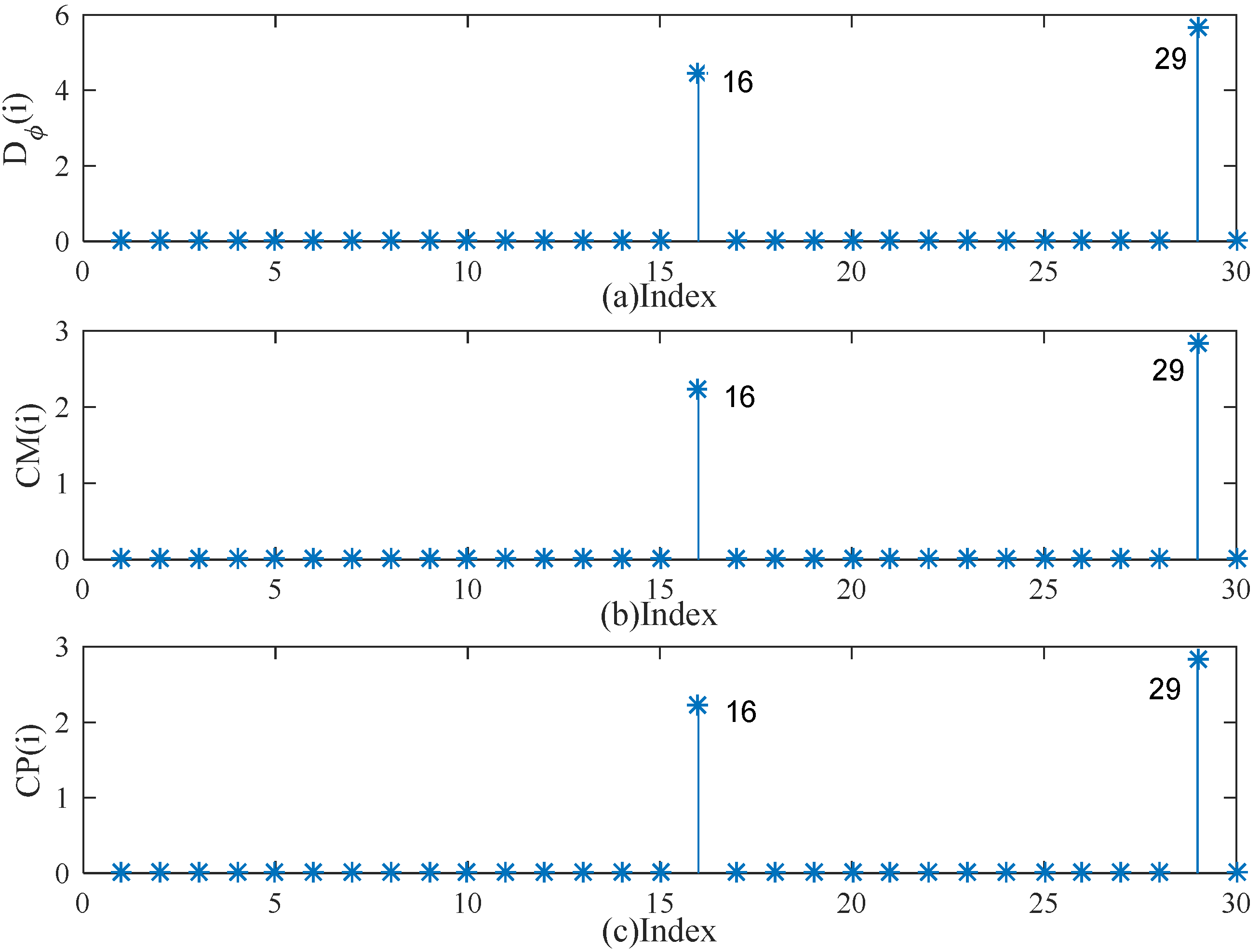
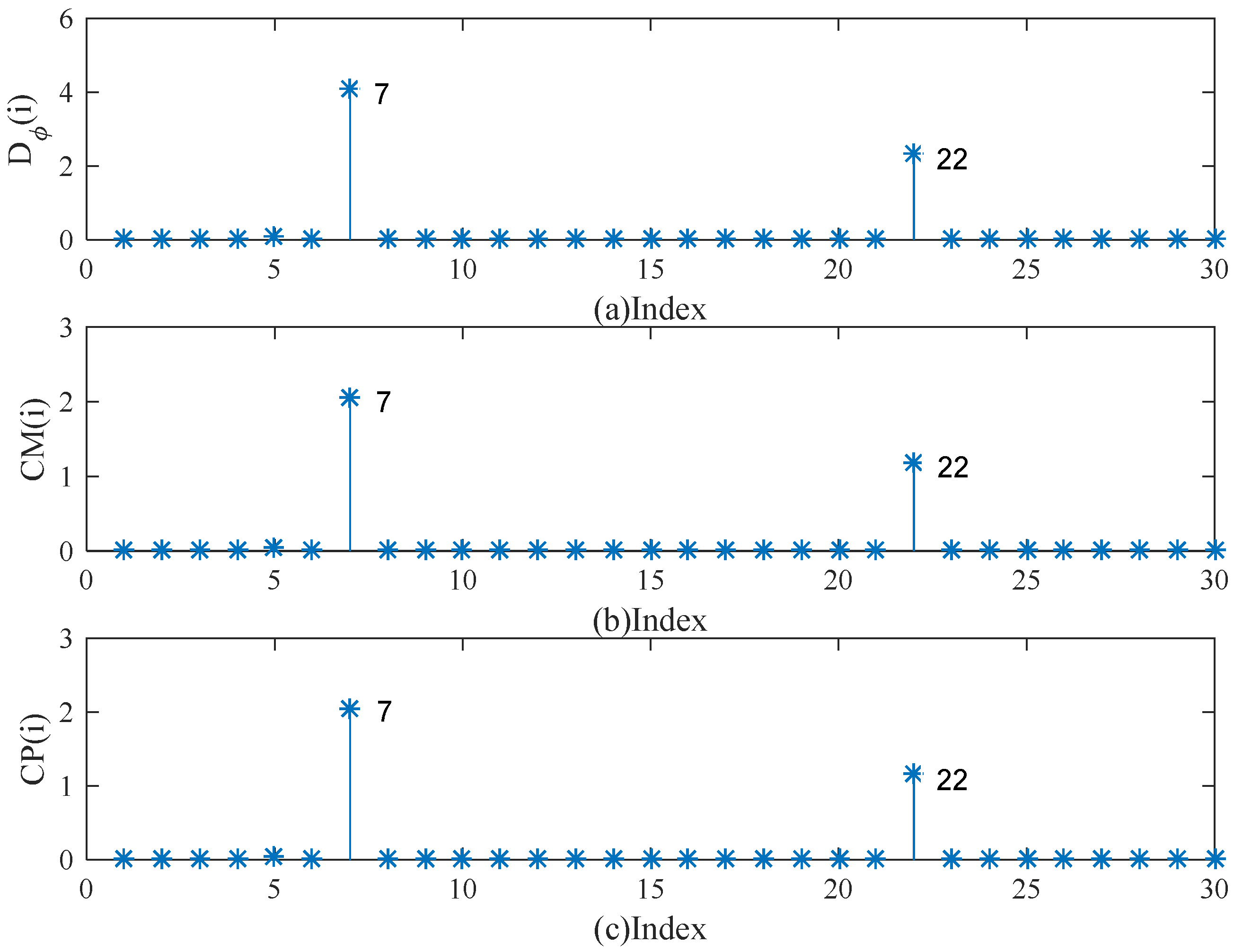
3. Bayesian Local Influence Analysis

This section uses the Bayesian local influence analysis method to evaluate the impact of small perturbations in the data, prior distribution and sample distribution on the posterior distribution in the SSARMs.

3.1. Perturbation Model and Manifold

Following Zhu et al. [14], the following perturbation model with skew-normal spatial data is considered:

$$p(\mathit{Y},\mathit{\theta }|\mathit{X},\mathit{\omega })=p(\mathit{\theta }|{\mathit{\omega }}_p)p(\mathit{Y}|\mathit{X},\mathit{\theta },{\mathit{\omega }}_d,{\mathit{\omega }}_s)$$

(6)

and ${\int }^{ }p(\mathit{Y},\mathit{\theta }|\mathit{X},\mathit{\omega })d\mathit{Y}d\mathit{\theta }=1$, where $\mathit{Y}={(y_1,\dots ,y_n)}^T$ is a $n\times 1$ dimensional dependent variables vector of expression (1), ${\mathit{\omega }}_p\in {\mathit{\Re }}^{k_p}$ represents the perturbations to the prior, ${\mathit{\omega }}_d\in {\mathit{\Re }}^{k_d}$ represents the perturbations to the data and ${\mathit{\omega }}_s\in {\mathit{\Re }}^{k_s}$ represents the perturbations to sampling distribution. Denote $k=k_p+k_d+k_s$. Suppose ${\mathit{\omega }}^0={({\mathit{\omega }}_p^{0^T},{\mathit{\omega }}_d^{0^T},{\mathit{\omega }}_s^{0^T})}^T\in {\mathit{\Re }}^k$ represents no perturbation.

Similar to Zhu et al. [14], the perturbed model $\mathit{ℳ}=\{p(\mathit{Y},\mathit{\theta }|\mathit{X},\mathit{\omega }):\mathit{\omega }\in {\mathit{\Re }}^k\}$ is regarded as the $k$-dimensional manifold under some regular conditions. The tangent space ${\mathit{T}}_{\omega }$ of $\mathit{ℳ}$ at each $\omega \in \mathit{ℳ}$ is spanned by $k$ functions ${\partial }_{{\omega }_q}\ell \left(\mathit{\omega }\right)$, where ${\partial }_{{\omega }_q}=\partial /\partial {\omega }_q$, $\ell \left(\mathit{\omega }\right)=\log p(\mathit{Y},\mathit{\theta }|\mathit{X},\mathit{\omega })$ and ${\omega }_q$ is the $q$th element of $\mathit{\omega }$. So,

$$g_{iq}\left(\mathit{\omega }\right)=E_{\omega }\left\{{\partial }_{{\omega }_j}\ell \left(\mathit{\omega }\right){\partial }_{{\omega }_q}\ell \left(\mathit{\omega }\right)\right\}=E_{\omega }\left\{-{\partial }_{{\omega }_j{\omega }_q}^2\ell \left(\mathit{\omega }\right)\right\}, j,q=1,\cdots ,k.$$

(7)

where ${\partial }_{{\omega }_j{\omega }_q}^2\ell \left(\mathit{\omega }\right)={\partial }^2\ell \left(\mathit{\omega }\right)/\partial {\omega }_j\partial {\omega }_q$, the expectation of the joint probability density function $p(\mathit{Y},\mathit{\theta }|\mathit{X},\mathit{\omega })$ is denoted as $E_{\omega }$. The diagonal element $g_{jj}\left(\mathit{\omega }\right)$ is considered to measure the amount of perturbation ${\omega }_j$ and the quantity $r_{iq}=g_{jq}\left(\mathit{\omega }\right)/\sqrt{g_{jj}\left(\mathit{\omega }\right)g_{qq}\left(\mathit{\omega }\right)}$ is considered to measure the association between perturbations ${\omega }_j$ and ${\omega }_q$. If $\mathit{G}\left({\mathit{\omega }}^0\right)$ is a diagonal matrix, all elements of $\mathit{\omega }$ are mutually orthogonal and the relevant perturbation is referred to as a suitable perturbation. If $\mathit{G}\left({\mathit{\omega }}^0\right)$ is not a diagonal matrix, the relevant perturbation is referred to as an improper perturbation. However, we can always find an appropriate perturbation vector $\tilde{\mathit{\omega }}={\mathit{\omega }}^0+{\left\{\mathit{G}\left({\mathit{\omega }}^0\right)\right\}}^{\frac{1}{2}}\left(\mathit{\omega }-{\mathit{\omega }}^0\right)$ such that $\mathit{G}\left(\tilde{\mathit{\omega }}\right)$ evaluated at ${\mathit{\omega }}^0$ equals $c{\mathit{I}}_k$, where $c$ is a positive number.

The Bayesian local influence analysis method is designed to quantify the degree of dependence of the posterior distribution on these three key elements of Bayesian analysis, including the prior distribution, the sampling distribution and the data. To illustrate the effect of small perturbations of the prior distribution, the sampling distribution and the data on SSARMs, the following four forms of perturbation are considered. The perturbation of covariate is considered in Example 1. The perturbation of the dependent variable is considered in Example 2. The perturbation of the prior distribution is considered in Example 3. The perturbation of the sampling distribution is considered in Example 4.

Example 1.

The Bayesian perturbation model for thespatialdata includes many perturbation schemes. The perturbation scheme to data points is proposed for identifying outliers and influential observations.Consider the perturbation covariate $\mathit{X}: \mathit{X}\left({\mathit{\omega }}_x\right)={({\mathit{X}}_1+{\omega }_1{\mathbf{1}}_p,\dots ,{\mathit{X}}_n+{\omega }_n{\mathbf{1}}_p)}^T=\mathit{X}+{\mathit{\omega }}_x{\mathbf{1}}_p^T$, in which ${\mathit{\omega }}_x={({\omega }_1,\dots ,{\omega }_n)}^T$,${\mathbf{1}}_p={(1,\dots ,1)}^T$is a $p\times 1$vector and ${\mathit{\omega }}_x^0={(0,\dots ,0)}^T$stands for no perturbation. A Riemann manifold is formed by a perturbation model $\mathit{ℳ}=\{p(\mathit{Y},\mathit{\theta }|\mathit{X},{\mathit{\omega }}_x):{\mathit{\omega }}_x\mathit{\in }{\Re }^n\}$. The tangent space ${\mathit{T}}_{{\omega }_x}$of $\mathit{ℳ}$can be spanned by

$${\partial }_{{\omega }_x}\ell \left({\mathit{\omega }}_x\right)={({\mathbf{1}}_p^T\mathit{\beta })}^T{({\sigma }_{\epsilon }^2{\mathit{I}}_n)}^{-1}\left[\mathit{Y}-\rho \mathit{W}\mathit{Y}-\left(\mathit{X}+{\mathit{\omega }}_x{\mathbf{1}}_p^T\right)\mathit{\beta }-{\mathit{\delta }}_{\epsilon }{\mathit{R}}_{\epsilon }\right],$$

(8)

when ${\mathit{\omega }}_x={\mathit{\omega }}_x^0$. We have

$${\partial }_{{\omega }_x}\ell \left({\mathit{\omega }}_x^0\right)={({\mathbf{1}}_p^T\mathit{\beta })}^T{({\sigma }_{\epsilon }^2{\mathit{I}}_n)}^{-1}\left(\mathit{Y}-\rho \mathit{W}\mathit{Y}-\mathit{X}\mathit{\beta }-{\mathit{\delta }}_{\epsilon }{\mathit{R}}_{\epsilon }\right).$$

(9)

It is easily shown that$\mathit{G}\left({\mathit{\omega }}_x^0\right)=E\left\{-{\partial }_{{\omega }_x}^2\ell \left({\mathit{\omega }}_x^0\right)\right\}={({\mathbf{1}}_p^T\mathit{\beta })}^T{({\sigma }_{\epsilon }^2{\mathit{I}}_n)}^{-1}\left({\mathbf{1}}_p^T\mathit{\beta }\right)$. When$\mathit{G}\left({\mathit{\omega }}_x^0\right)$is a diagonal matrix, the perturbation is referred to as a suitable perturbation. Otherwise, the perturbation is deemed to be inappropriate.

Example 2.

Bayesian local influence analysis methods have many more perturbation schemes for spatial data points. In Example 1, perturbations of $\mathit{X}$are considered. However, perturbations of the dependent variable $\mathit{Y}$also have an impact on the Bayesian analysis. Consider the perturbation to the response variables $\mathit{Y}$:$\mathit{Y}\left({\mathit{\omega }}_y\right)={(y_1+{\omega }_1,\dots ,y_n+{\omega }_n)}^T=\mathit{Y}+{\mathit{\omega }}_y$, in which ${\mathit{\omega }}_y={({\omega }_1,\dots ,{\omega }_n)}^T$and ${\mathit{\omega }}_y^0={(0,\dots ,0)}^T$stands for no perturbation. A Riemann manifold is formed by a perturbation model $\mathit{ℳ}=\{p(\mathit{Y},\mathit{\theta }|\mathit{X},{\mathit{\omega }}_y):{\mathit{\omega }}_y\in {\mathit{\Re }}^n\}$. The tangent space ${\mathit{T}}_{{\omega }_y}$of $\mathit{ℳ}$can be spanned by

$${\partial }_{{\omega }_y}\ell \left({\mathit{\omega }}_y\right)={({\mathit{I}}_n-\rho \mathit{W})}^T{({\sigma }_{\epsilon }^2{\mathit{I}}_n)}^{-1}[\tilde{\mathit{Y}}\left({\mathit{\omega }}_y\right)-\mathit{X}\mathit{\beta }-{\mathit{\delta }}_{\epsilon }{\mathit{R}}_{\epsilon },$$

(10)

in which $\tilde{\mathit{Y}}\left({\mathit{\omega }}_y\right)=\mathit{Y}+{\mathit{\omega }}_y-\rho \mathit{W}\left(\mathit{Y}+{\mathit{\omega }}_y\right)$. When${\mathit{\omega }}_y={\mathit{\omega }}_y^0$, we have

$${\partial }_{{\omega }_y}\ell \left({\mathit{\omega }}_y^0\right)={({\mathit{I}}_n-\rho \mathit{W})}^T{({\sigma }_{\epsilon }^2{\mathit{I}}_n)}^{-1}\left(\mathit{Y}-\rho \mathit{W}\mathit{Y}-\mathit{X}\mathit{\beta }-{\mathit{\delta }}_{\epsilon }{\mathit{R}}_{\epsilon }\right).$$

(11)

It is easily shown that$\mathit{G}\left({\mathit{\omega }}_y^0\right)=E\left\{-{\partial }_{{\omega }_y}^2\ell \left({\mathit{\omega }}_y^0\right)\right\}={({\mathit{I}}_n-\rho \mathit{W})}^T{({\sigma }_{\epsilon }^2{\mathit{I}}_n)}^{-1}\left({\mathit{I}}_n-\rho \mathit{W}\right)$. When$\mathit{G}\left({\mathit{\omega }}_y^0\right)$is a diagonal matrix, the perturbation is referred to as a suitable perturbation. Otherwise, the perturbation is deemed to be inappropriate.

Example 3.

The Bayesian perturbation model for the prior distribution includes many existing schemes.Consider the perturbation to the prior distribution of $\mathit{\beta }$:$p(\mathit{\beta }|{\omega }_{\beta })\sim N\left({\omega }_{\beta }\mathit{\beta },{\mathit{M}}_{\beta }\right)$, in which ${\omega }_{\beta }$is a positive number. Additionally, ${\omega }_{\beta }^0=1$stands for no perturbation. A Riemann manifold is formed by a perturbation model $\mathit{ℳ}=\{p(\mathit{Y},\mathit{\theta }|\mathit{X},{\omega }_{\beta }):{\omega }_{\beta }\in {\mathit{\Re }}^1\}$. The tangent space ${\mathit{T}}_{{\omega }_{\beta }}$of $\mathit{ℳ}$can be spanned by

$${\partial }_{{\omega }_{\beta }}\ell \left({\omega }_{\beta }\right)={\mathit{\beta }}_0^T{({\mathit{M}}_{\beta })}^{-1}\left(\mathit{\beta }-{\omega }_{\beta }{\mathit{\beta }}_0\right).$$

(12)

It is easily shown that$\mathit{G}\left({\omega }_{\beta }^0\right)=E\left\{-{\partial }_{{\omega }_{\beta }}^2\ell \left({\omega }_{\beta }^0\right)\right\}={\mathit{\beta }}_0^T{({\mathit{M}}_{\beta })}^{-1}{\mathit{\beta }}_0$. When$\mathit{G}\left({\omega }_{\beta }^0\right)$is a diagonal matrix, the perturbation is referred to as a suitable perturbation. Otherwise, the perturbation is deemed to be inappropriate.

Example 4.

The Bayesian perturbation model for the sampling distribution includes many perturbation schemes. Consider the perturbation to the distribution of the disturbances $\mathit{\epsilon }$:$p(\mathit{\epsilon }|{\omega }_{\epsilon })\sim S{N}_n\left(\mathbf{0},{\sigma }_{\epsilon }^2{\mathit{I}}_n,{\omega }_{\epsilon }{\delta }_{\epsilon }{\mathit{I}}_n\right)$, in which ${\omega }_{\epsilon }$is a scalar and ${\omega }_{\epsilon }^0=1$means no perturbation. A Riemann manifold is formed by a perturbation model $\mathit{ℳ}=\{p(\mathit{Y},\mathit{\theta }|\mathit{X},{\omega }_{\epsilon }):{\omega }_{\epsilon }\in {\mathit{\Re }}^1\}$. The tangent space ${\mathit{T}}_{{\omega }_{\epsilon }}$of$\mathit{ℳ}$is spanned by

$${\partial }_{{\omega }_{\epsilon }}\ell \left({\omega }_{\epsilon }\right)={({\delta }_{\epsilon }{\mathit{R}}_{\epsilon })}^T{({\sigma }_{\epsilon }^2{\mathit{I}}_n)}^{-1}\left(\mathit{Y}-\rho \mathit{W}\mathit{Y}-\mathit{X}\mathit{\beta }-{\omega }_{\epsilon }{\delta }_{\epsilon }{\mathit{R}}_{\epsilon }\right).$$

(13)

It is easily shown that$\mathit{G}\left({\omega }_{\epsilon }^0\right)=E\left\{-{\partial }_{{\omega }_{\epsilon }}^2\ell \left({\omega }_{\epsilon }^0\right)\right\}={({\delta }_{\epsilon }{\mathit{R}}_{\epsilon })}^T{({\sigma }_{\epsilon }^2{\mathit{I}}_n)}^{-1}\left({\delta }_{\epsilon }{\mathit{R}}_{\epsilon }\right)$. When$\mathit{G}\left({\omega }_{\epsilon }^0\right)$is a diagonal matrix, the perturbation is referred to as a suitable perturbation. Otherwise, the perturbation is deemed to be inappropriate.

3.2. Local Influence Measures

Following Zhu et al. [14], let objective function $f\left(\mathit{\omega }\right):\mathit{ℳ}\to {\mathit{\Re }}^r$ be the objective function. The influence of perturbation can be measured by considering the Bayes factor, $\varphi$-divergence and posterior mean distance. If $\mathit{\omega }\left(t\right)$ is a geodesic on the finite dimensional manifold $\mathit{ℳ}$ with $\mathit{\omega }\left(0\right)={\mathit{\omega }}^0$ and ${\partial }_t\mathit{\omega }\left(t\right){|}_{t=0}=\mathit{h}\in {\mathit{\Re }}^m$, in practice, the geodesic can be taken as ${\mathit{\omega }}^0=t\mathit{h}$. The Taylor expansion of objective function $f\left(\mathit{\omega }\left(t\right)\right)$ at $t=0$ is $f\left(\mathit{\omega }\left(t\right)\right)=f\left(\mathit{\omega }\left(0\right)\right)+{\dot{f}}_h\left(0\right)t+O\left(t^2\right)$, where ${\dot{f}}_h\left(0\right)={\mathbf{\nabla }}_f^T\mathit{h}$, ${\mathbf{\nabla }}_f=\partial f\left(\mathit{\omega }\right)/\partial \mathit{\omega }$ and $\mathit{h}=d\mathit{\omega }\left(t\right)/dt{|}_{t=0}\in {\mathit{\Re }}^m$.

Firstly, when ${\mathbf{\nabla }}_f\ne 0$, the first-order influence measure in the defined direction $\mathit{h}\in {\mathit{\Re }}^m$ is

$$\mathit{F}{\mathit{I}}_{f,h}=\mathit{F}{\mathit{I}}_{f\left(\omega \left(0\right)\right),h}=\frac{{\mathit{h}}^T{\mathbf{\nabla }}_f{\mathit{W}}_f{\mathbf{\nabla }}_f^T\mathit{h}}{{\mathit{h}}^T\mathit{G}\mathit{h}},$$

(14)

where $\mathit{G}=\mathit{G}\left({\mathit{\omega }}^0\right)$, ${\mathit{W}}_f$ represents a positive semi-definite matrix. Notably, the first-order influence measure can be rewritten with appropriate perturbations $\tilde{\mathit{\omega }}\left(\mathit{\omega }\right)$, then further defined as

$$\mathit{F}{\mathit{I}}_{f\left(\tilde{\omega }\right),h|\tilde{\omega }={\omega }^0}={\mathit{h}}^T{\mathit{G}}^{-\frac{1}{2}}{\mathbf{\nabla }}_f{\mathit{W}}_f{\mathbf{\nabla }}_f^T{\mathit{G}}^{-\frac{1}{2}}\mathit{h}.$$

(15)

Following Poon and Poon [25], the first-order adjusted influence measure $\mathit{F}\mathit{I}{\mathit{C}}_{f\left({\tilde{\omega }}^0\right),h}$ can be defined as

$$\mathit{F}\mathit{I}{\mathit{C}}_{f\left({\tilde{\omega }}^0\right),h}={\mathit{h}}^T\mathit{ℬ}\mathit{h},$$

(16)

in which $\mathit{ℬ}=\mathit{Q}/\mathrm{tr}\left(\mathit{Q}\right)$ in which $\mathit{Q}={\mathit{G}}^{-\frac{1}{2}}{\mathbf{\nabla }}_f{\mathit{W}}_f{\mathbf{\nabla }}_f^T{\mathit{G}}^{-\frac{1}{2}}$, $\mathrm{tr}\left(A\right)$ denotes the trace of a matrix $A$.

Let ${\eta }_1\ge \dots {\eta }_t>0$ be the non-zero eigenvalues of matrix $\mathit{ℬ}$ and ${\mathit{u}}_1,\dots ,{\mathit{u}}_t$ be the corresponding orthogonal eigenvectors, where ${\mathit{u}}_i={(u_{i1},\dots ,u_{ik})}^T$ for $i=1,\dots ,\iota$. The local maximum influence degree $\tilde{\omega }$ is reflected by the maximum eigenvalue ${\mathsf{\eta }}_1$. The corresponding eigenvector ${\mathit{u}}_1$ is the direction of the most significant perturbations showing the perturbations of the three components of the SSARMs to obtain the largest local variation in $\mathit{f}\left({\mathit{\omega }}^0\right)$ and further identify influential observations, misspecified priors and insufficient sampling distributions. Regrettably, it is not sufficient to assess ${\mathit{u}}_1$ local impacts by inspection alone (Poon and Poon [25]). Through their arguments, local influence is evaluated using the overall contribution vector of all eigenvectors associated with all non-zero eigenvalues: $\mathit{M}\left(0\right)={\eta }_1{\mathit{u}}_1^2+\dots +{\eta }_t{\mathit{u}}_t^2$, where ${\mathit{u}}_i^2={(u_{i1}^2,\dots ,u_{ik}^2)}^T$. It is easy to show that the $j$th component of $\mathit{M}\left(0\right)$ is $M{(0)}_j=\sum _{i=1}^{\iota }{\eta }_i{u}_{ij}^2=FI{C}_{f\left({\tilde{\omega }}^0\right),v_j}$, for $j=1,\dots ,k$, where $v_j$ is a $k\times 1$ primary perturbation vector, the 𝑗th element is 1, the rest of the features are 0 and $b_{jj}$ is the $j$th diagonal element of matrix $\mathit{ℬ}$. Similar to Zhu et al. [14], $\overline{M}\left(0\right)+2SM\left(0\right)$ is considered as a benchmark, where $\overline{M}\left(0\right)$ is the mean of $\{M{(0)}_j:j=1,\dots ,k\}$ and $SM\left(0\right)$ is the standard error of $\{\mathit{M}{(0)}_j:j=1,\dots ,k\}$. That is to say, if $\overline{M}\left(0\right)+2SM\left(0\right)\le {\mathrm{b}}_{jj}$, the $j$th observation is identified as an influential point.

Example 5 (Bayes factor).

In this example, the perturbation change is measured by the Bayes factor. It measures this change mainly by the difference between $log\{p(\mathit{Y}|{\mathit{\omega }}^0)\}$without perturbation and $log\{p(\mathit{Y}|\mathit{\omega })\}$with perturbation. Consider objective function as the Bayes factor: $f\left(\mathit{\omega }\right)=log\{p(\mathit{Y}|\mathit{\omega })\}-log\{p(\mathit{Y}|{\mathit{\omega }}^0)\}$, where $p(\mathit{Y}|\mathit{\omega })=log{\int }^{ }p(\mathit{Y},\mathit{\theta }|\mathit{X},\mathit{\omega })d\mathit{\theta }$. It is easy to prove that

$${\mathbf{\nabla }}_B={\mathit{E}}_{\theta |Y,X,{\omega }^0}\{{\partial }_{\omega }logp(\mathit{Y},\mathit{\theta }|\mathit{X},{\mathit{\omega }}^0)\left|\mathit{Y}\right\}\ne 0,$$

(17)

in which ${\mathbf{\nabla }}_B$ can be approximated by${\mathbf{\nabla }}_B\approx {\mathcal{S}}^{-1}\sum _{s=1}^{\mathcal{S}}{\partial }_{\omega }logp(\mathit{Y},{\mathit{\theta }}^{\left(s\right)}|\mathit{X},{\mathit{\omega }}^0)$and$\left\{{\mathit{\theta }}^{\left(s\right)}:s=1,\dots ,\mathcal{S}\right\}$ is generated via the MCMC algorithm, unifying theGibbs sampler with the MH algorithm.

Secondly, when ${\mathbf{\nabla }}_f=0$, the second-order Taylor expansion of the objective function $f\left(\mathit{\omega }\right)$ is $f\left(\mathit{\omega }\left(t\right)\right)=f\left(\mathit{\omega }\left(0\right)\right)+0.5{\ddot{f}}_h\left(0\right)t^2+O\left(t^3\right)$, where ${\ddot{f}}_h\left(0\right)={\mathit{h}}^T{\mathit{H}}_f\mathit{h}$ and ${\mathit{H}}_f={\partial }_{\omega }^{2}f\left(\mathit{\omega }\right){|}_{\omega ={\omega }^0}$. Similar to Zhu et al. [14], the second-order influence measure in the direction $\mathit{h}\in {\mathit{\Re }}^m$ is given as

$$\mathit{S}{\mathit{I}}_{f,h}=\mathit{S}{\mathit{I}}_{f\left(\omega \left(0\right)\right),h}=\frac{{\mathit{h}}^T{\mathit{H}}_f\mathit{h}}{{\mathit{h}}^T\mathit{G}\mathit{h}}.$$

(18)

In particular, when the appropriate perturbation $\tilde{\mathit{\omega }}\left(\mathit{\omega }\right)$ is added, the second-order influence measure can be further simplified as

$$\mathit{S}{\mathit{I}}_{f\left(\tilde{\omega }\right),h|\tilde{\omega }={\omega }^0}={\mathit{h}}^T{\mathit{G}}^{-\frac{1}{2}}{\mathit{H}}_f{\mathit{G}}^{-\frac{1}{2}}\mathit{h}.$$

(19)

Therefore, the second-order adjusted influence measure can be defined as

$$\mathit{S}\mathit{C}{\mathit{I}}_{f\left({\tilde{\omega }}^0\right),h}={\mathit{h}}^T{\mathit{ℬ}}_s\mathit{h},$$

(20)

in which ${\mathit{ℬ}}_s={\mathit{Q}}_s/\mathrm{tr}\left({\mathit{Q}}_s\right)$, ${\mathit{Q}}_s={\mathit{G}}^{-\frac{1}{2}}{\mathit{H}}_f{\mathit{G}}^{-\frac{1}{2}}$. The largest eigenvalue of ${\mathit{ℬ}}_s$ is an important indicator to evaluate the local influence behavior of the model and the corresponding eigenvector is the direction of the most significant local influence, which reveals how the three elements of SSARMs are perturbed and can be identified as the potential influence points, erroneous priors and improper modelling assumptions.

Example 6 ($\mathit{\varphi }$-divergence). 

In this example, the perturbation change is measured by the $\varphi$-divergence. It measures this change mainly by the difference between two posterior probability density functions. Setting the objective function $f\left(\mathit{\omega }\right)$between the two posterior probability density functions before and after the introduction of perturbation $\mathit{\omega }$as $\varphi$-divergence can be defined as

$$D_{\varphi }\left(\mathit{\omega }\right)={\int }^{ }\varphi (R(\mathit{\theta }|\mathit{Y},\mathit{X},\mathit{\omega }))p(\mathit{\theta }|\mathit{Y},\mathit{X})d\mathit{\theta },$$

(21)

where$R(\mathit{\theta }|\mathit{Y},\mathit{X},\mathit{\omega })=\frac{p(\mathit{\theta }|\mathit{Y},\mathit{X},\mathit{\omega })}{p(\mathit{\theta }|\mathit{Y},\mathit{X})}$and$\varphi (\cdot )$is a convex function with$\varphi \left(1\right)=0$. It is easy to prove that ${\mathbf{\nabla }}_{\varphi }=0$and

$${\mathit{H}}_{\varphi }=\ddot{\varphi }\left(1\right)[E_{{\omega }^0}{\{{\partial }_{\omega }logp(\mathit{Y},\mathit{\theta }|\mathit{X},{\mathit{\omega }}^0)\}}^{\otimes 2}-{\{E_{{\omega }^0}{\partial }_{\omega }logp(\mathit{Y},\mathit{\theta }|\mathit{X},{\mathit{\omega }}^0)\}}^{\otimes 2}],$$

(22)

where$a^{\otimes 2}=a{a}^T$. ${\mathit{H}}_{\varphi }$is difficult to calculate directly because it involves higher dimensional integrals. To solve this problem, the approximate expression of${\mathit{H}}_{\varphi }$can be written as

$${\mathit{H}}_{\varphi }\approx \ddot{\varphi }\left(1\right)\left[\frac{1}{\mathcal{S}}{\sum }_{s=1}^{\mathcal{S}}{\{{\partial }_{\omega }logp(\mathit{Y},{\mathit{\theta }}^{\left(s\right)}|\mathit{X},{\mathit{\omega }}^0)\}}^{\otimes 2}-{\left(\frac{1}{\mathcal{S}}{\sum }_{s=1}^{\mathcal{S}}{\partial }_{\omega }logp\left(\mathit{Y},{\mathit{\theta }}^{\left(s\right)}|\mathit{X},{\mathit{\omega }}^0\right)\right)}^{\otimes 2}\right].$$

(23)

Example 7 (Posterior Mean Distance).

In this example, the perturbation change is measured by Cook’s posterior mean distance. It measures this change mainly by the difference between two posterior means. Consider the objective function $f\left(\mathit{\omega }\right)$as Cook’s posterior mean distance between two posterior means of known function $g\left(\mathit{\theta }\right)$before and after the introduction of perturbation $\mathit{\omega }$, which is defined as

$$C{M}_g\left(\mathit{\omega }\right)={\{{\mathit{Q}}_g\left(\mathit{\omega }\right)-{\mathit{Q}}_g\left({\mathit{\omega }}^0\right)\}}^T{\mathit{G}}_g\left\{{\mathit{Q}}_g\left(\mathit{\omega }\right)-{\mathit{Q}}_g\left({\mathit{\omega }}^0\right)\right\},$$

(24)

where${\mathit{Q}}_g\left(\mathit{\omega }\right)={\int }^{ }g\left(\mathit{\theta }\right)p(\mathit{\theta }|\mathit{Y},\mathit{X},\mathit{\omega })d\mathit{\theta }$ is the posterior mean of$g\left(\mathit{\theta }\right)$and${\mathit{G}}_g={[var\{g\left(\mathit{\theta }\right)|\mathit{Y},\mathit{X},{\mathit{\omega }}^0\}]}^{-1}$. It is easily shown that${\mathbf{\nabla }}_{CM}=0$and${\mathit{H}}_{CM}={\mathit{Q}}_g^{*T}{\mathit{G}}_g{\mathit{Q}}_g^{*}$, where${\mathit{Q}}_g^{*}={cov}_{{\omega }^0}\{g\left(\mathit{\theta }\right),{\partial }_{\omega }logp(\mathit{Y},\mathit{\theta }|\mathit{X},{\mathit{\omega }}^0)\}$, which can be approximated by

$$\begin{gathered} {\mathit{Q}}_g^{*}\approx {\mathcal{S}}^{-1}{\displaystyle \sum }_{s=1}^{\mathcal{S}}\{g\left({\mathit{\theta }}^{\left(s\right)}\right){\partial }_{\omega }\log p(\mathit{Y},{\mathit{\theta }}^{\left(s\right)}|\mathit{X},{\mathit{\omega }}^0)\} \\ -\left({\mathcal{S}}^{-1}{\displaystyle \sum }_{s=1}^{\mathcal{S}}g\left({\mathit{\theta }}^{\left(s\right)}\right)\right)\left({\mathcal{S}}^{-1}{\displaystyle \sum }_{s=1}^{\mathcal{S}}{\partial }_{\omega }\log p(\mathit{Y},{\mathit{\theta }}^{\left(s\right)}|\mathit{X},{\mathit{\omega }}^0)\right). \end{gathered}$$

(25)

For the above considered objective functions and perturbation schemes, the following steps are used to achieve Bayesian local influence analysis.

Step 1. A Bayesian perturbation model $p(\mathit{Y},\mathit{\theta }|\mathit{X},\mathit{\omega })$ is constructed.

Step 2.${\mathbf{\nabla }}_f={\partial }_{\omega }f\left(\mathit{\omega }\left(0\right)\right)$, ${\mathit{H}}_f={\partial }_{\omega }^{2}f\left(\mathit{\omega }\right){|}_{\omega ={\omega }^0}$ and $\mathit{G}=\mathit{G}\left({\mathit{\omega }}^0\right)$ are calculated.

Step 3. If ${\mathbf{\nabla }}_f\ne 0$, the local effects of small perturbations are evaluated by computing the influence measure $\mathit{F}\mathit{C}{\mathit{I}}_{f\left({\tilde{\omega }}^0\right),{\mathit{e}}_j}$ of the first-order adjustment. However, if ${\mathbf{\nabla }}_f=0$, the second-order adjusted influence measure $\mathit{S}\mathit{C}{\mathit{I}}_{f\left({\tilde{\omega }}^0\right),e_j}$ is calculated.

Step 4. For some given objective functions $f\left(\mathit{\omega }\right)$, if $M{(0)}_j=\mathit{F}\mathit{C}{\mathit{I}}_{f\left({\tilde{\omega }}^0\right),e_j}\ge \overline{M}\left(0\right)+2SM\left(0\right)$ or $M{(0)}_j=\mathit{S}\mathit{C}{\mathit{I}}_{f\left({\tilde{\omega }}^0\right),e_j}\ge \overline{M}\left(0\right)+2SM\left(0\right)$, the $j$th observation is detected as an influential observation.

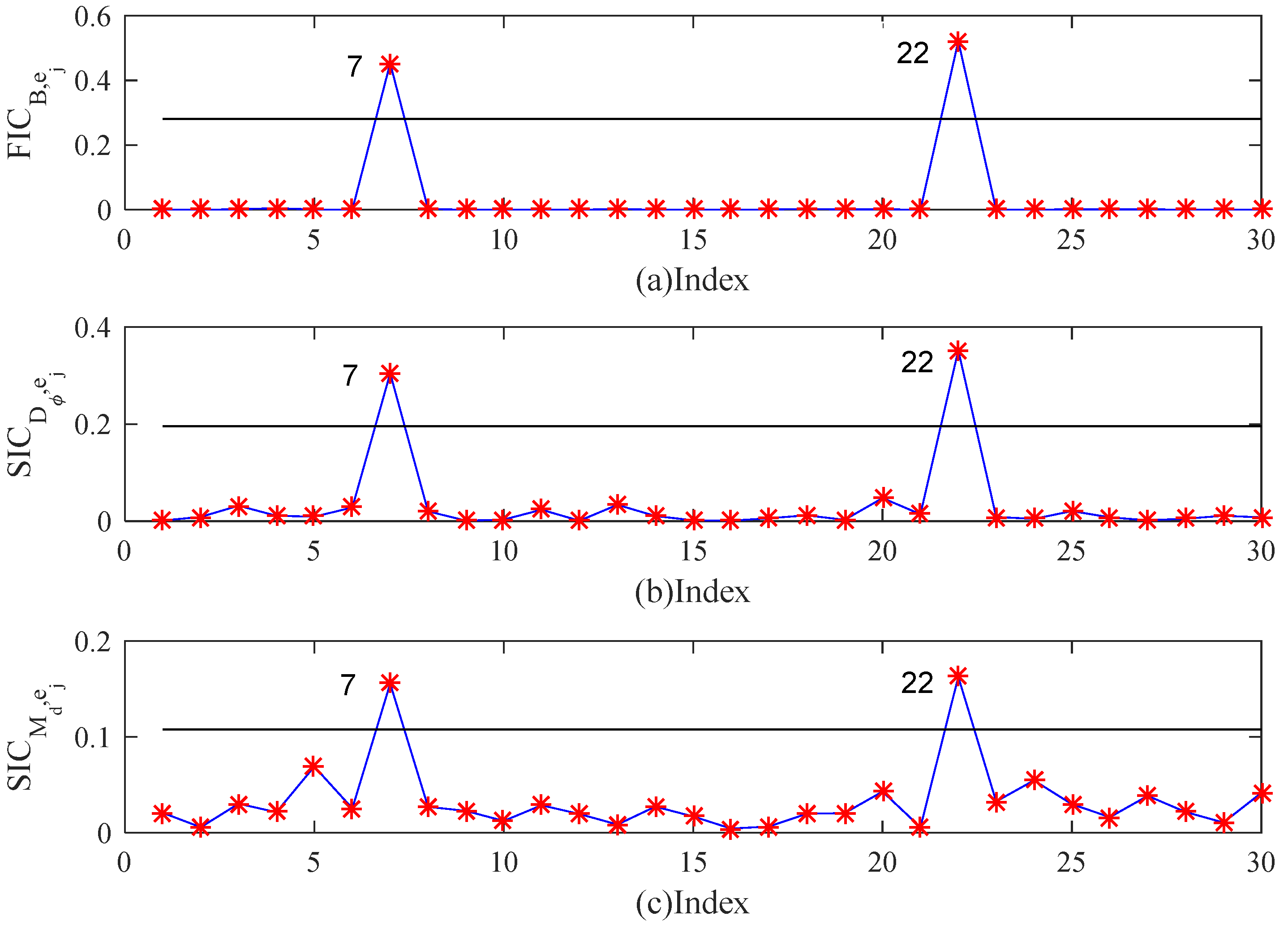
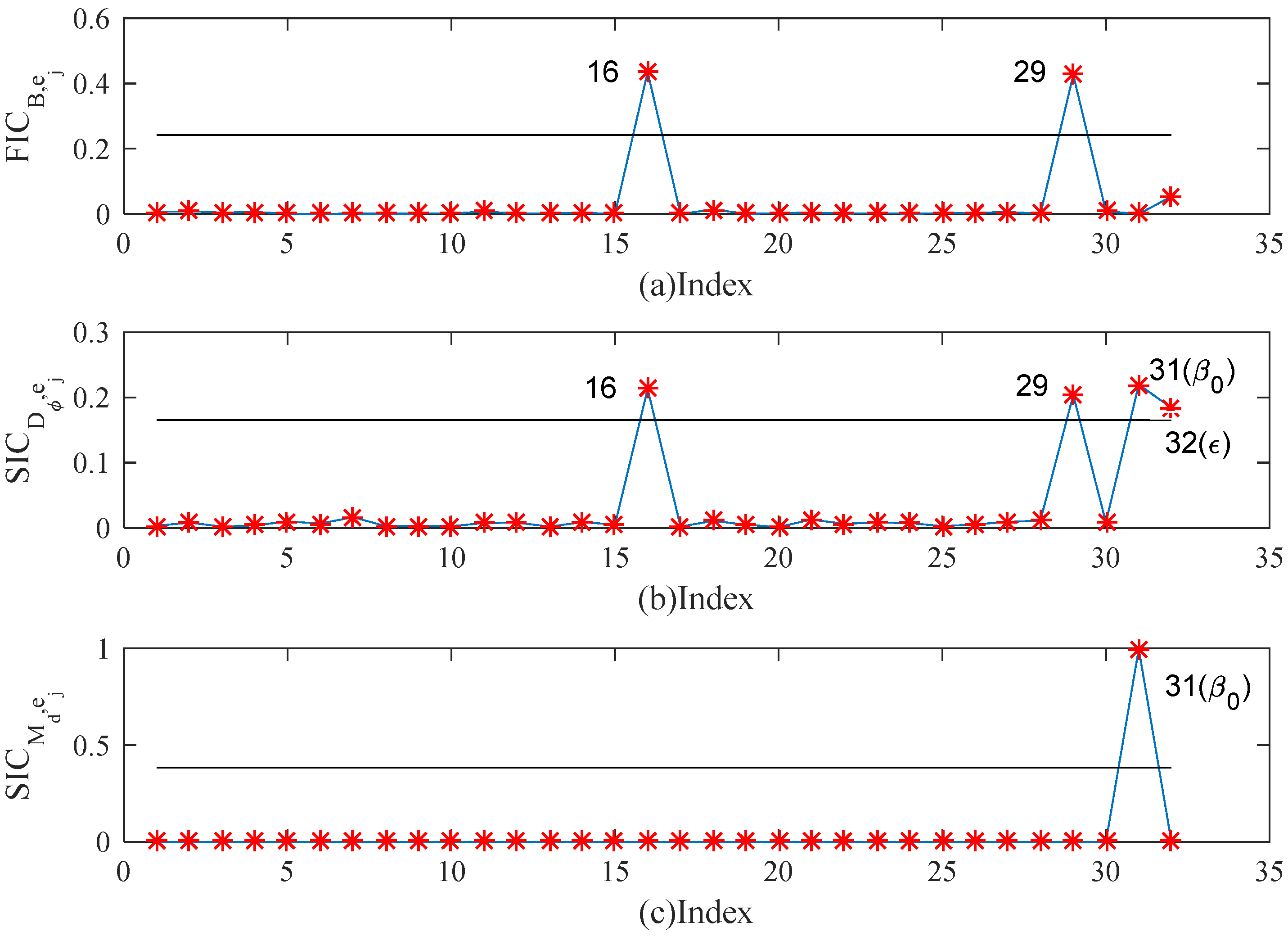
4. Bayesian Case Influence Analysis

According to the case deletion approach provided by Cook and Weisberg [26,27], three Bayesian case influence measures are considered in this section. Let ${\mathit{Y}}_S$ and ${\mathit{X}}_S$ denote subsamples of $\mathit{Y}$ and $\mathit{X}$, respectively, for which all observations are in $S$. Let ${\mathit{Y}}_{\left[S\right]}$ and ${\mathit{X}}_{\left[S\right]}$ represent subsamples of $\mathit{Y}$ and $\mathit{X},$ respectively, and delete all observations in ${\mathit{Y}}_S$ and ${\mathit{X}}_S$.

To order to measure the impact of deleting observations in $\left\{{\mathit{Y}}_S,{\mathit{X}}_S\right\}$ on the posterior distribution of $\mathit{\theta }$, the first type of Bayesian case influence measure is the $\varphi$-influence of ${\mathit{Y}}_{\left[S\right]}$, defined as

$$D_{\varphi }\left(S\right)={\int }^{ }\varphi \left(R_{\left[S\right]}\left(\mathit{\theta }\right)\right)p(\mathit{\theta }|\mathit{Y},{\mathit{X}}_{\left[S\right]})d\mathit{\theta },$$

(26)

where $\varphi (\cdot )$ is a convex function with $\varphi \left(1\right)=0$, and $R_{\left[S\right]}\left(\mathit{\theta }\right)=p(\mathit{\theta }|{\mathit{Y}}_{\left[S\right]})/p(\mathit{\theta }|\mathit{Y})$. $D_{\varphi }\left(S\right)$ measures the difference between $p(\mathit{\theta }|{\mathit{Y}}_{\left[S\right]},{\mathit{X}}_{\left[S\right]})$ and $p(\mathit{\theta }|\mathit{Y},\mathit{X})$posterior distributions. If $D_{\varphi }\left(S\right)$ is large, the observations in $S$ are detected to be influential.

In order to measure the impact of deleting observations in $S$ on the posterior mean of $\mathit{\theta }$, the second type of Bayesian case influence measure that Cook’s posterior mean distance, denoted by $CM\left(S\right)$, is considered as:

$$CM\left(S\right)={({\tilde{\mathit{\theta }}}_{\left[S\right]}-\tilde{\mathit{\theta }})}^T{\mathit{W}}_{\theta }\left({\tilde{\mathit{\theta }}}_{\left[S\right]}-\tilde{\mathit{\theta }}\right),$$

(27)

where ${\mathit{W}}_{\theta }$ is a positive definite matrix and can be seen as the inverse of $\mathit{\theta }$’s posterior covariance matrix. $\tilde{\mathit{\theta }}={\int }^{ }\mathit{\theta }p(\mathit{\theta }|\mathit{Y})d\mathit{\theta }$and ${\tilde{\mathit{\theta }}}_{\left[S\right]}={\int }^{ }\mathit{\theta }p(\mathit{\theta }|{\mathit{Y}}_{\left[\mathit{S}\right]})d\mathit{\theta }$are the posterior means of $\mathit{\theta }$ based on data $\mathit{Y}$ and ${\mathit{Y}}_{\left[S\right]}$, respectively. If the value of $CM\left(S\right)$ is large, it points out that deleting observations in $S$ will have a significant impact on the posterior mean. Therefore, the observations in $S$ are considered to be strong influence points.

In order to measure the impact of deleting observations in $S$ on the posterior mode of $\mathit{\theta }$, the third type of Bayesian case influence measure is Cook’s posterior mode distance, denoted by $CP\left(S\right)$, which is considered as:

$$CP\left(S\right)={({\widehat{\mathit{\theta }}}_{\left[S\right]}-\widehat{\mathit{\theta }})}^T{\mathit{G}}_{\theta }\left({\widehat{\mathit{\theta }}}_{\left[S\right]}-\widehat{\mathit{\theta }}\right),$$

(28)

where, ${\mathit{G}}_{\theta }$ is a positive definite matrix and $\widehat{\mathit{\theta }}={\mathrm{argmax}}_{\theta }logp(\mathit{\theta }|\mathit{Y})$ and ${\widehat{\mathit{\theta }}}_{\left[S\right]}={\mathrm{argmax}}_{\theta }\log p(\mathit{\theta }|{\mathit{Y}}_{\left[S\right]})$ represent the posterior mode of parameter $\mathit{\theta }$concerning $\mathit{Y}$ and ${\mathit{Y}}_{\left[S\right]}$, respectively. If the value of $CP\left(S\right)$ is large, it indicates that deleting observations in $S$ will have a significant impact on the posterior mode. Therefore, the observations in $S$ are considered strong influence points.

To obtain $D_{\varphi }\left(S\right)$, $CM\left(S\right)$ and $CP\left(S\right)$, it is necessary to calculate $p(\mathit{\theta }|\mathit{Y})$ and $p(\mathit{\theta }|{\mathit{Y}}_{\left[S\right]})$. When $p_S\left(\mathit{\theta }\right)=p(\mathit{Y}|\mathit{\theta })/p({\mathit{Y}}_{\left[S\right]}|\mathit{\theta })=p({\mathit{Y}}_S|\mathit{\theta })$, it is easily shown that

$$p\left(\mathit{\theta }|{\mathit{Y}}_{\left[S\right]}\right)=\frac{{\left\{p_S\left(\mathit{\theta }\right)\right\}}^{-1}p(\mathit{\theta }|\mathit{Y})}{{\int }^{ }{\left\{p_S\left(\mathit{\theta }\right)\right\}}^{-1}p\left(\mathit{\theta }|\mathit{Y}\right)d\mathit{\theta }} ,$$

(29)

where $R_{\left[S\right]}\left(\mathit{\theta }\right)=\left\{p_S\left(\mathit{\theta }\right)\right\}{ }^{-1}/E_{\mathit{\theta }|\mathit{Y}}{\left\{p_S\left(\mathit{\theta }\right)\right\}}^{-1}$. Thus, $D_{\varphi }\left(S\right)$ can be written as

$$D_{\varphi }\left(S\right)={\mathrm{E}}_{\mathit{\theta }|\mathit{Y}}\left[\varphi \left(\frac{{\left\{p_S\left(\mathit{\theta }\right)\right\}}^{-1}}{E_{\mathit{\theta }|\mathit{Y}}{\left\{p_S\left(\mathit{\theta }\right)\right\}}^{-1}}\right)\right],$$

(30)

where ${\mathrm{E}}_{\mathit{\theta }|\mathit{Y}}$ represents the mathematical expectation of the posterior distribution $p(\mathit{\theta }|\mathit{Y})$. The K-L divergence $\left(\varphi \left(k\right)=-\log (k\right))$, $D_{\varphi }\left(S\right)=\log {\mathrm{E}}_{\mathit{\theta }|\mathit{Y}}{\left\{p_S\left(\mathit{\theta }\right)\right\}}^{-1}+{\mathrm{E}}_{\mathit{\theta }|\mathit{Y}}\left\{\log p_S\left(\mathit{\theta }\right)\right\}$ can be considered a computational formula of $D_{\varphi }\left(S\right)$. To compute $CM\left(S\right)$, we need to evaluate $\tilde{\mathit{\theta }}$ and ${\tilde{\mathit{\theta }}}_{\left[S\right]}$. Where $\tilde{\mathit{\theta }}={\mathrm{E}}_{\mathit{\theta }|\mathit{Y}}\left(\mathit{\theta }\right)$ and ${\tilde{\mathit{\theta }}}_{\left[S\right]}={\mathrm{E}}_{\mathit{\theta }|\mathit{Y}}(\mathit{\theta }{\left\{p_S\left(\mathit{\theta }\right)\right\}}^{-1})/{\mathrm{E}}_{\mathit{\theta }|\mathit{Y}}{\left\{p_S\left(\mathit{\theta }\right)\right\}}^{-1}$. In order to obtain $CP\left(S\right)$, it is necessary to calculate $\widehat{\mathit{\theta }}$ and ${\widehat{\mathit{\theta }}}_{\left[S\right]}$. Typically, the posterior mode of $\mathit{\theta }$ is not a closed-form, so an iterative algorithm is needed to obtain $\widehat{\mathit{\theta }}$ and ${\widehat{\mathit{\theta }}}_{\left[S\right]}$. ${\mathit{G}}_{\theta }$ in $CP\left(S\right)$ can be analytically obtained by evaluating $\mathit{J}\left(\mathit{\theta }\right)=-{\partial }_{\theta }^2\log p(\mathit{\theta }|\mathit{Y})=-{\partial }_{\theta }^2\log p(\mathit{Y}|\mathit{\theta })-{\partial }_{\theta }^2\log p\left(\mathit{\theta }\right)$ at $\widehat{\mathit{\theta }}$. ${\mathit{W}}_{\theta }$ can be obtained by computing the value of ${\mathit{J}}_{\theta }$ at $\mathit{\theta }$, which can also be equal to the inverse of the posterior covariance matrix of θ. Thus, $D_{\varphi }\left(S\right)$, $CM\left(S\right)$ and $CP\left(S\right)$ are derived directly by averaging MCMC samples over the posterior distribution $p(\mathit{\theta }|\mathit{Y})$.

5. Simulation Studies and Real Examples

The proposed approaches in Section 3 and Section 4 will be illustrated by three simulation studies and practical cases of air quality from China (2020) in this section.

5.1. Simulation Studies

The data set $\left\{y_i:i=1,\cdots ,n\right\}$ was generated from Equation (1) with $n=30$ and $p=3$. $\mathit{X}$ was generated from the normal distribution $N\left(\mathbf{0},{\mathit{I}}_{30}\right)$; the measurement errors $\mathit{\epsilon }$ were generated from the skew-normal distribution $\mathit{\epsilon }~S{N}_{30}\left(\mathbf{0},{\sigma }_{\epsilon }^2{\mathit{I}}_{30},{\delta }_{\epsilon }{\mathit{I}}_{30}\right)$. The spatial weight matrix $\mathit{W}$ was generated from the Delaunay program in MATLAB. The true values of $\rho$, $\mathit{\beta }$, ${\delta }_{\epsilon }$ and ${\sigma }_{\epsilon }^2$ were taken to be $\rho =0.2$, $\mathit{\beta }={(1.25,2,1.2)}^T$, ${\delta }_{\epsilon }=0.1$ and ${\sigma }_{\epsilon }^2=0.1$, respectively. The hyperparameters of ${\mathit{\beta }}_0$, ${\mathit{M}}_{\mathit{\beta }}$, ${\delta }_{\epsilon 0}$, $M_{{\delta }_{\epsilon }}$, $v_0$ and $s_0$ were taken to be ${\mathit{\beta }}_0={(1.25,2,1.2)}^T$, ${\mathit{M}}_{\mathit{\beta }}=0.001{\mathit{I}}_3$, ${\delta }_{\epsilon 0}=0.1$, $M_{{\delta }_{\epsilon }}=0.001$, $v_0=6$ and $s_0=2$, respectively. Such true values of the parameters were selected randomly. The purpose of selecting parameter values is only to test whether the proposed method is effective. The hyperparameters of the prior distribution were selected to be similar to the true value to make the algorithm converge quickly.

To illustrate the previously proposed Bayesian theory of local influence analysis, the following two simulation studies were considered.

Simulation 1.

In this simulation study, the outliers were generated in the following two ways (i) $x_{16}$was changed to $x_{16}+2$and $x_{29}$was changed to $x_{29}+2$, and (ii) $y_7$was changed to $y_7+8$and $y_{22}$was changed to $y_{22}+8$. For case (i), for the covariate perturbation in Example 1, the Bayesian local influence measures$\mathit{F}\mathit{I}{\mathit{C}}_{B,e_j}$,$\mathit{S}\mathit{I}{\mathit{C}}_{D_{\varphi },e_j}$and $\mathit{S}\mathit{I}{\mathit{C}}_{M_d,e_j}$were calculated by using an MCMC algorithm iteration 10,000 times, discarding the first 5000 times and using the last 5000 iteration values to calculate them. The results are shown in Figure 1a–c, respectively. Cases 16 and 29 turned out to be influential observations, as we expected. For case (ii), for the response variables perturbation in Example 2, the Bayesian local influence measures $\mathit{F}\mathit{I}{\mathit{C}}_{B,e_j}$, $\mathit{S}\mathit{I}{\mathit{C}}_{D_{\varphi },e_j}$and $\mathit{S}\mathit{I}{\mathit{C}}_{M_d,e_j}$were calculated by using an MCMC algorithm iteration 10,000 times, discarding the first 5000 times and using the last 5000 iteration values to calculate them. The results are shown in Figure 2a–c, respectively. Cases 7 and 22 turned out to be influential observations, as expected.

Simulation 2.

In this simulation study, perturbations to the data, priors and sampling distribution were considered simultaneously. The outliers generation method was similar to the first method in Simulation 1. (i) The covariate perturbations were considered (see Example 1), (ii) the prior distribution of $\mathit{\beta }$perturbations was considered (see Example 3) and (iii) the distributions of $\mathit{\epsilon }$perturbations were considered (see Example 4). The perturbed log-likelihood function is shown as follows

$$\begin{gathered} \log p\left(\mathit{Y},\mathit{\theta }|\mathit{\omega }\right)\propto -\frac{1}{2}{(\mathit{Y}-\rho \mathit{W}\mathit{Y}-{\mathit{X}}_{\omega }\mathit{\beta }-{\delta }_{\epsilon }{\mathit{R}}_{\epsilon })}^T{({\sigma }_{\epsilon }^2{\mathit{I}}_n)}^{-1}\left(\mathit{Y}-\rho \mathit{W}\mathit{Y}-{\mathit{X}}_{\omega }\mathit{\beta }-{\delta }_{\epsilon }{\mathit{R}}_{\epsilon }\right)-\frac{1}{2}{(\mathit{\beta }-{\omega }_{\beta }{\mathit{\beta }}_0)}^T{\mathit{M}}_{\beta }^{-1}\left(\mathit{\beta } \\ -{\omega }_{\beta }{\mathit{\beta }}_0\right)-\frac{1}{2}{(\mathit{Y}-\rho \mathit{W}\mathit{Y}-\mathit{X}\mathit{\beta }-{\omega }_{\epsilon }{\delta }_{\epsilon }{\mathit{R}}_{\epsilon })}^T{({\sigma }_{\epsilon }^2{\mathit{I}}_n)}^{-1}\left(\mathit{Y}-\rho \mathit{W}\mathit{Y}-\mathit{X}\mathit{\beta }-{\omega }_{\epsilon }{\delta }_{\epsilon }{\mathit{R}}_{\epsilon }\right) \end{gathered}$$

where$\mathit{\omega }={({\omega }_1,\dots ,{\omega }_{30},{\omega }_{\beta },{\omega }_{\epsilon })}^T$and${\mathit{X}}_{\omega }=\mathit{X}+{\mathit{\omega }}_x{\mathbf{1}}_p^T$. In this case,${\mathit{\omega }}^0={(0,\dots ,0,1,1)}^T$represents no perturbation. After some calculations, we obtained$\mathit{G}\left({\mathit{\omega }}^0\right)=diag\left(a_{11},a_{22},a_{33}\right)$, where$a_{11}={\mathit{\beta }}^T{\mathbf{1}}_p{({\sigma }_{\epsilon }^2{\mathit{I}}_n)}^{-1}{\mathbf{1}}_p^T\mathit{\beta }$,$a_{22}={\mathit{\beta }}_0^T{\mathit{M}}_{\beta }^{-1}{\mathit{\beta }}_0$and$a_{33}={({\delta }_{\epsilon }{\mathit{R}}_{\epsilon })}^T{({\sigma }_{\epsilon }^2{\mathit{I}}_n)}^{-1}{\delta }_{\epsilon }{\mathit{R}}_{\epsilon }$. The Bayesian local influence measures$\mathit{F}\mathit{I}{\mathit{C}}_{B,e_j}$,$\mathit{S}\mathit{I}{\mathit{C}}_{D_{\varphi },e_j}$and$\mathit{S}\mathit{I}{\mathit{C}}_{M_d,e_j}$were concluded using an MCMC algorithm iteration 10,000 times, discarding the first 5000 times and using the last 5000 iteration values to calculate them based on prior distribution$N\left(10{\mathit{\beta }}_0,{\mathit{M}}_{\beta }\right)$of$\mathit{\beta }$and the distributions$S{N}_{30}\left(\mathbf{0},{\sigma }_{\epsilon }^2{\mathit{I}}_n,30{\delta }_{\epsilon }{\mathit{R}}_{\epsilon }\right)$of$\mathit{\epsilon }$. The results are shown inFigure 3a–c. The results showed that cases 16 and 29 were identified to be influential observations, and the prior distribution of$\mathit{\beta }$and distributions of$\mathit{\epsilon }$were detected to be misspecified distributions with having a large effect on$\mathit{F}\mathit{I}{\mathit{C}}_{B,e_j}$,$\mathit{S}\mathit{I}{\mathit{C}}_{D_{\varphi },e_j}$and$\mathit{S}\mathit{I}{\mathit{C}}_{M_d,e_j}$.

To demonstrate the Bayesian case influence diagnostics methods, we consider the following simulation research:

Simulation 3.

In this simulation research, the outliers were generated in the following two ways (i) $x_{16}$was changed to $x_{16}+2$and $x_{29}$was changed to $x_{29}+2$, and (ii) $y_7$was changed to $y_7+8$and $y_{22}$was changed to $y_{22}+8$. The Bayesian case influence measures $D_{\varphi }\left(S\right)$,$CM\left(S\right)$and $CP\left(S\right)$were calculated using an MCMC algorithm iteration 10,000 times, discarding the first 5000 times and using the last 5000 iteration values to calculate them. The results are shown in Figure 4a–c and Figure 5a–c. In this simulation, samples 16 and 29 are created as outliers for $x$and the other points as normal. Therefore, results are correct when samples 16 and 29 are detected to be outliers and the other points are less influenced or have no influence. Similarly, samples 7 and 22 are creased as outliers for $y$and the other points as normal. Therefore, the results are correct when samples 7 and 22 are detected to be outliers and the other points are less influenced or have no influence. It can be seen from Figure 4 that cases 16 and 29 were detected to be influential; it can be seen from Figure 5 that cases 7 and 22 were diagnosed as influence points. As we expected, the results are the same as the previous diagnosis of Bayesian local influence measures.

5.2. Real Example

A dataset concerning China’s air quality was used to demonstrate our proposed approach in the subsection. Let ${\mathit{X}}_p$ be a $31\times 1$ vector of the fine particulate matter (PM_2.5) in 31 provinces, let ${\mathit{X}}_s$ be a $31\times 1$ vector of the sulfur dioxide (SO₂) in 31 provinces, let ${\mathit{X}}_c$ be a $31\times 1$ vector of the carbon monoxide (CO) in 31 provinces and let $\mathit{Y}={(y_1,\dots ,y_{31})}^T$ be a $31\times 1$ vector of the air quality index (AQI) in 31 provinces.

Firstly, the above data were exploited to illustrate the application of the Bayesian local influence analysis method. The following three perturbation options were considered: (i) perturbations to covariates; (ii) perturbations to response variables; (iii) covariates, prior distributions of $\mathit{\beta }$ and sampling distributions of $\mathit{\epsilon }$ are perturbed simultaneously. Bayesian local influence measures $\mathit{F}\mathit{I}{\mathit{C}}_{B,e_j}$, $\mathit{S}\mathit{I}{\mathit{C}}_{D_{\varphi },e_j}$ and $\mathit{S}\mathit{I}{\mathit{C}}_{M_d,e_j}$ were calculated for three different perturbation scenarios. The results are shown in Figure 6, Figure 7 and Figure 8. The results of Figure 6a–c show that cases 6 and 19 were diagnosed as influence points by $\mathit{F}\mathit{I}{\mathit{C}}_{B,e_j}$, $\mathit{S}\mathit{I}{\mathit{C}}_{D_{\varphi },e_j}$ and $\mathit{S}\mathit{I}{\mathit{C}}_{M_d,e_j}$ in perturbation scheme (i). The results of Figure 7a–c show that cases 1 and 12 were diagnosed as influence points by $\mathit{F}\mathit{I}{\mathit{C}}_{B,e_j}$, $\mathit{S}\mathit{I}{\mathit{C}}_{D_{\varphi },e_j}$ and $\mathit{S}\mathit{I}{\mathit{C}}_{M_d,e_j}$ in perturbation scheme (ii). The results of Figure 8a,b show that cases 6 and 19 were diagnosed as influence points by $\mathit{F}\mathit{I}{\mathit{C}}_{B,e_j}$, $\mathit{S}\mathit{I}{\mathit{C}}_{D_{\varphi },e_j}$ and $\mathit{S}\mathit{I}{\mathit{C}}_{M_d,e_j}$ in perturbation scheme (iii). The results of Figure 8b show that the prior distribution of $\mathit{\beta }$, the distributions of $\mathsf{\epsilon }$ were diagnosed to have a significant effect by $\mathit{S}\mathit{I}{\mathit{C}}_{D_{\varphi },e_j}$. The results of Figure 8c showed that the prior distribution of $\mathit{\beta }$ was diagnosed to have a significant effect by $\mathit{S}\mathit{I}{\mathit{C}}_{M_d,e_j}$.

Secondly, the above data are used to illustrate the application of the Bayesian case influence analysis method. We calculated Bayesian case influence measures $D_{\varphi }\left(S\right)$, $CM\left(S\right)$ and $CP\left(S\right)$. The results are presented in Figure 9 and Figure 10. Figure 9a–c demonstrate that cases 6 and 19 were diagnosed as influence points. Figure 10a–c demonstrate that cases 1 and 12 were diagnosed as influence points. As we expected, the results are the same as the previous diagnosis of Bayesian local influence measures.

Finally, by reviewing China’s air quality data for April 2020, it was found that cases 6 and 19’s influence points represent Harbin and Shenyang, respectively. In particular, Harbin’s air quality is the second-lowest among the 31 provincial capitals in China, while Shenyang’s air quality is the third-lowest among the 31 provincial capitals in China. This indicates that the air quality situation in these two cities is more prominent among the 31 provinces. Similarly, it was found that cases 1 and 12 of the diagnosed impact points represented Beijing and Lhasa, respectively. Among them, Beijing’s air quality ranks 17th among 31 provincial capital cities. The air quality of Lhasa ranks fourth among the 31 provinces, indicating that the air quality of Lhasa is indeed outstanding among the 31 provincial capital cities. Although Beijing’s air quality ranks in the middle of the 31 provincial capitals, there are many sandstorms in Beijing in April, which will lead to abnormal air quality in Beijing. It is further illustrated that the impact point diagnosed is consistent with the relevant air quality reality.

To further illustrate that the observed values of samples 6 and 19 may be the outliers, the parameter estimates before and after deleting the 6th and 19th observations are calculated, respectively, as shown in

Table 1. Bayesian estimation with or without influence point 6 and 19 in the real example.

Par.	With		Without
	Est.	SD.	Est.	SD.
${\beta }_1$	1.1988	0.0315	1.3440	0.0311
${\beta }_2$	1.9275	0.0320	2.1451	0.0315
${\beta }_3$	1.1440	0.0315	1.2767	0.0313
$\rho$	0.1795	0.1348	0.4755	0.2005
${\sigma }_{\epsilon }^2$	1.0437	0.1023	1.3488	0.1430
${\delta }_{\epsilon }$	0.0979	0.0076	0.0000	0.0000

. Table 1 show that after deleting the 6th and 19th observations, the estimators of ${\beta }_1,{\beta }_2,{\beta }_3,\rho ,{\sigma }_{\epsilon }^2,{\delta }_{\epsilon }$ are changed from 1.1988, 1.9275, 1.1440, 0.1795, 1.0437, 0.0979 to 1.3440, 2.1451, 1.2767, 0.4755, 1.3488, 0.0000, respectively. Similarly, to further illustrate that the observed values of samples 1 and 12 are the outliers, the parameter estimates before and after deleting the 1st and 12th observations are calculated, respectively, as shown in

Table 2. Bayesian estimation with or without influence point 1 and 12 in the real example.

Par.	With		Without
	Est.	SD.	Est.	SD.
${\beta }_1$	1.1988	0.0315	0.9898	0.0316
${\beta }_2$	1.9275	0.0320	1.5838	0.0314
${\beta }_3$	1.1440	0.0315	0.9491	0.0315
$\rho$	0.1795	0.1348	0.2086	0.1701
${\sigma }_{\epsilon }^2$	1.0437	0.1023	3.2987	0.7886
${\delta }_{\epsilon }$	0.0979	0.0076	0.1989	0.0019

. Table 2 show that after deleting the 1st and 12th observations, the estimators of ${\beta }_1,{\beta }_2,{\beta }_3,\rho ,{\sigma }_{\epsilon }^2,{\delta }_{\epsilon }$ are changed from 1.1988, 1.9275, 1.1440, 0.1795, 1.0437, 0.0979 to 0.9898, 1.5838, 0.9491, 0.2086, 3.2987, 0.1989, respectively.

6. Discussion

Based on SSARMs with response variables obeying skew-normal distribution, this paper proposed a Bayesian local influence method to evaluate the impact of small perturbations in data, prior distribution and sample distribution. Perturbation models with separate or simultaneous perturbations of covariates, response variables, parameter prior and sample distributions were developed. A Bayesian perturbation manifold was constructed to describe the internal structure of perturbation models and quantify the perturbation degree of different perturbation models. The Bayesian local influence measures, including the Bayes factor, the $\varphi$-distance and the posterior mean distance, were used to evaluate the impact of various perturbations. In addition, three Bayesian case deletion influence measures, including $\varphi$-distance, Cook’s posterior mean distance and Cook’s posterior mode distance, were proposed to identify potential outliers in skew-normal spatial autoregression models. The effectiveness of our proposed approach was illustrated by three simulation studies and a real example. The results showed that: (1) our proposed Bayesian local influence approach can effectively identify the potential influence points, misspecified prior distribution and misspecified sampling distribution; (2) our proposed Bayesian case influence approach can be used to effectively detect the potential influence observations; (3) the outliers detected by the Bayesian local influence approach and Bayesian case influence approach are consistent, which further explains the rationality of the two methods.

References

1. LeSage, J.; Pace, R.K. Introduction to Spatial Econometrics; Chapman and Hall: London, UK, 2009. [Google Scholar]
2. Piribauer, P.; Cuaresma, J.C. Bayesian variable selection in spatial autoregressive models. Spat. Econ. Anal. 2016, 11, 457–479. [Google Scholar] [CrossRef]
3. Xie, T.F.; Cao, R.Y.; Du, J. Variable selection for spatial autoregressive models with a diverging number of parameters. Stat. Pap. 2018, 61, 1125–1145. [Google Scholar] [CrossRef]
4. Du, J.; Sun, X.Q.; Cao, R.Y.; Zhang, Z.Z. Statistical inference for partially linear additive spatial autoregressive models. Spat. Stat.-Neth. 2018, 25, 52–67. [Google Scholar] [CrossRef]
5. Xie, L.; Wang, X.R.; Cheng, W.H.; Tang, T. Variable selection for spatial autoregressive models. Commun. Stat.-Theor. Methods 2019, 50, 1325–1340. [Google Scholar] [CrossRef]
6. Jay, M.; Ver, H.; Erin, E.; Peterson, M.B.; Hooten, E.M.; Hanks, M.J.F. Spatial autoregressive models for statistical inference from ecological data. Ecol. Monogr. 2018, 88, 36–59. [Google Scholar]
7. Anik, A.; Bambang, W.O.; Purhadi, P.; Sutikno, S. Lagrange multiplier test for spatial autoregressive model with latent variables. Symmetry 2020, 12, 1375. [Google Scholar]
8. Song, Y.Q.; Liang, X.J.; Zhu, Y.J.; Lin, L. Robust variable selection with exponential squared loss for the spatial autoregressive model. Comput. Stat. Data Anal. 2021, 155. [Google Scholar] [CrossRef]
9. Pereira, M.A.A.; Russo, C.M. Nonlinear mixed-effects models with scale mixture of skew-normal distributions. J. Appl. Stat. 2019, 46, 1602–1620. [Google Scholar] [CrossRef]
10. Yin, J.H.; Wu, L.C.; Dai, L. Variable selection in finite mixture of regression models using the skew-normal distribution. J. Appl. Stat. 2020, 47, 2941–2960. [Google Scholar] [CrossRef]
11. Tatsuya, K.; Strawderman, W.E.; Ryota, Y. Shrinkage estimation of location parameters in a multivariate skew-normal distribution. Commun. Stat.-Theor. Methods 2020, 49, 2008–2024. [Google Scholar]
12. Liu, Y.H.; Mao, G.; Leiva, V.; Liu, S.Z.; Alejandra, T. Diagnostic analytics for an autoregressive model under the skew-normal distribution. Mathematics 2020, 8, 693. [Google Scholar] [CrossRef]
13. Teimouri, M. EM algorithm for mixture of skew-normal distributions fitted to grouped data. J. Appl. Stat. 2021, 48, 1154–1179. [Google Scholar] [CrossRef]
14. Zhu, H.T.; Ibrahim, J.G.; Tang, N.S. Bayesian influence analysis: A geometric approach. Biometrika 2011, 98, 307–323. [Google Scholar] [CrossRef] [PubMed]
15. Zhang, Y.Q.; Tang, N.S. Bayesian local influence analysis of general estimating equations with nonignorable missing data. Comput. Stat. Data Anal. 2017, 105, 184–200. [Google Scholar] [CrossRef]
16. Ouyang, M.; Yan, X.D.; Chen, J.; Tang, N.S.; Song, X.Y. Bayesian local influence of semiparametric structural equation models. Comput. Stat. Data Anal. 2017, 111, 102–115. [Google Scholar] [CrossRef]
17. Dai, X.W.; Jin, L.B.; Tian, M.Z.; Shi, L. Bayesian local influence for spatial autoregressive models with heteroscedasticity. Stat. Pap. 2019, 60, 1423–1446. [Google Scholar] [CrossRef]
18. Ju, Y.Y.; Tang, N.S.; Li, X.X. Bayesian local influence analysis of skew-normal spatial dynamic panel data models. J. Stat. Comput. Sim. 2018, 88, 2342–2364. [Google Scholar] [CrossRef]
19. Vicente, G.; Cancho, D.K.D.; Victor, H.; Lachos, M.G.A. Bayesian nonlinear regression models with scale mixtures of skew-normal distributions: Estimation and case influence diagnostics. Comput. Stat. Data Anal. 2010, 55, 588–602. [Google Scholar]
20. Zhu, H.T.; Joseph, G.I.; Cho, Y.; Tang, N.S. Bayesian case influence measures for statistical models with missing data. J. Comput. Graph. Stat. 2012, 21, 253–271. [Google Scholar] [CrossRef] [Green Version]
21. Tang, N.S.; Duan, X.D. Bayesian influence analysis of generalized partial linear mixed models for longitudinal data. J. Multivar. Anal. 2014, 126, 86–99. [Google Scholar] [CrossRef]
22. Hao, H.X.; Lin, J.G.; Wang, H.X.; Huang, X.F. Bayesian case influence analysis for GARCH models based on Kullback–Leibler divergence. J. Korean Stat. Soc. 2016, 45, 595–609. [Google Scholar] [CrossRef]
23. Duan, X.D.; Fung, W.F.; Tang, N.S. Bayesian semiparametric reproductive dispersion mixed models for non-normal longitudinal data: Estimation and case influence analysis. J. Stat. Comput. Sim. 2017, 87, 1925–1939. [Google Scholar] [CrossRef]
24. Arellano-Valle, R.B.; Bolfarine, H.; Lachos, V.H. Bayesian inference for skew-normal linear mixed models. J. Appl. Stat. 2007, 34, 663–682. [Google Scholar] [CrossRef]
25. Poon, W.Y.; Poon, Y.S. Conformal normal curvature and assessment of Local Influence. J. R. Stat. Soc. B 1999, 61, 51–61. [Google Scholar] [CrossRef]
26. Cook, R.D.; Weisberg, S. Residuals and influence regression. Biometrics 1982, 39, 413–415. [Google Scholar]
27. Weiss, R.E.; Cook, R.D. A graphical case statistic for assessing posterior influence. Biometrika 1992, 79, 51–55. [Google Scholar] [CrossRef]
Figure 1. Plots of covariate perturbation in Simulation 1.
Mathematics 10 01306 g001
Figure 2. Plots of response variables perturbation in Simulation 1.
Mathematics 10 01306 g002
Figure 3. Plots of simultaneous perturbation in Simulation 2.
Mathematics 10 01306 g003
Figure 4. Diagnostic plots of covariate outliers in Simulation 3.
Mathematics 10 01306 g004
Figure 5. Diagnostic plots of response variables outliers in Simulation 3.
Mathematics 10 01306 g005
Figure 6. Plots of covariate perturbation in the real example.
Mathematics 10 01306 g006
Figure 7. Plots of response variables perturbation in the real example.
Mathematics 10 01306 g007
Figure 8. Plots of simultaneous perturbation in the real example.
Mathematics 10 01306 g008
Figure 9. Diagnostic plots of covariate outliers in the real example.
Mathematics 10 01306 g009
Figure 10. Diagnostic plots of response variables outliers in the real example.
Mathematics 10 01306 g010