Mining Campus Big Data: Prediction of Career Choice Using Interpretable Machine Learning Method

Abstract

The issue of students’ career choice is the common concern of students themselves, parents, and educators. However, students’ behavioral data have not been thoroughly studied for understanding their career choice. In this study, we used eXtreme Gradient Boosting (XGBoost), a machine learning (ML) technique, to predict the career choice of college students using a real-world dataset collected in a specific college. Specifically, the data include information on the education and career choice of 18,000 graduates during their college years. In addition, SHAP (Shapley Additive exPlanation) was employed to interpret the results and analyze the importance of individual features. The results show that XGBoost can predict students’ career choice robustly with a precision, recall rate, and an F1 value of 89.1%, 85.4%, and 0.872, respectively. Furthermore, the interaction of features among four different choices of students (i.e., choose to study in China, choose to work, difficulty in finding a job, and choose to study aboard) were also explored. Several educational features, especially differences in grade point average (GPA) during their college studying, are found to have relatively larger impact on the final choice of career. These results can be of help in the planning, design, and implementation of higher educational institutions’ (HEIs) events.

1. Introduction

Educational data mining (EDM) is the application of data mining technology in the educational environment. With the development of modern information technologies, large amounts of educational data are stored in higher educational institutions (HEIs) even at the smallest granularity, such as daily attendance records. However, data storage alone is not sufficient for administrators and managers to make decisions. In response, colleges and universities actively promote the deep integration of artificial intelligence and education, fueling educational reform and innovation, which has become an inevitable trend to meet the development needs [1,2,3].

The decisions of HEIs include administrative or academic nature. Furthermore, the new goal of education in China requires universities to deeply grasp the patterns of students’ daily behavior, innovating the mode and methods involved in talent training, which is also a political task of promoting the deep integration of artificial intelligence and education and propelling educational reform as well as innovation. To achieve this goal, more efficient and user-friendly information-processing methods are needed to enable modern-day decision-making processes in HEIs [4].

Identity development primarily relates to career identity, which is mainly developed during adolescence [5]. A student’s professional identity may be shaped by adequate career exploration and continuous commitment in their college life [6]. Therefore, it is of great importance for universities to develop appropriate career counseling centers. The career counseling center will teach students some career planning methods or give some guidance according to students’ development needs. However, as we know, it is difficult for students to clearly determine their postgraduation destinations. From a psychological point of view, personal ideas and minds may vary greatly. This makes it difficult for HEIs to offer relevant services. With the development of information technology, in modern universities, the campus big data can be recorded through the campus information system. This means that all behavioral data of students on campus can be recorded in real time. Such behavior data can reflect the students’ learning process, unique habits, experiences, preferences, and state of mind. Therefore, analyzing campus big data through data mining technology can help students better understand themselves and solve the problem of employment difficulties.

Aiming to provide a practical insight into understanding students’ graduation decisions and their effect, we exploited machine learning techniques in a specific Chinese college. Specifically, we first constructed an optimal forecasting model based on an optimization method called Tree-structured Parzen Estimator (TPE) and XGBoost algorithm. Then, we used the Shapley Additivity explanation (SHAP) to explain the result obtained by the forecasting model. The main research work can be summarized as follows:

(1)

We use the supervised machine learning method, specifically XGBoost, to support decision making for HEIs based on real data analysis.

(2)

We performed a model optimization process to mitigate classification errors and to make complex ML models understandable.

(3)

We further put forward some policy to improve the operations of the education system and better serve students’ career choice.

Contribution

In our contributions, we have:

• Proposed a novel framework using interpretable machine learning method to identify the significant factors that affecting the students’ career choice;
• Obtained a real-world educational dataset containing four years of education records of 18,000 undergraduates in a specific college;
• Compared the performance of the proposed framework through state-of-the-art methods to validate the findings and further explored the obtained results to obtain a deep insight for students’ career choice;
• Proposed framework and policy suggestions to help HEIs and their managers for better understand their current world.

The rest of this paper is organized as follows. Section 2 reviews the literature, which presents the previous work related to EDM and reviews the literature about ML methods and conventional statistical techniques to approach high-dimensional educational data. Section 3 explains the materials and methods, including dataset collection, data cleaning, and modeling. Section 4 describes the obtained results using the interpretable machine learning method. Section 5 concludes the paper and highlights future work in this area of research.

2. Literature Review

2.1. Educational Data Mining

There are many methods and applications of EDM, and these studies can not only follow the application goal, such as improving learning quality, but also reach the theoretical goal, that is, to improve people’s understanding of the learning process. In addition, EDM applications can categorize end-users by targets. EDM can be applied to any stakeholders involved in the education system, such as students, teachers, managers, and researchers [7], also providing feedback, personalization, and recommendation, improving students’ learning process [8]. The application of EDM can also discover and provide a decision-support system that can help educators plan courses to improve teaching performance [9], providing administrators with resources and tools for decision making and organization [10]. Educational findings can help researchers better understand educational structures and assess learning effectiveness.

2.2. Machine Learning in Educational Area

Machine learning (ML) is a powerful approach for data mining and decision support among information technologies [11]. In terms of the education system, some notable examples include Accounting Systems [12], Enterprise Resource Planning [13,14], academic management [15], and prediction [16,17,18]. As a novel approach to improving schooling quality, HEIs need to predict and understand students’ graduation destination by analyzing students’ daily behavior.

Several studies used campus big data to predict students’ future. However, most of them focus on predicting/evaluating academic performance. Shaukat et al. [19,20,21] attempted to evaluate the students’ performance in a data mining perspective, and the performance of HEIs were found to be of importance in students’ performance. Amez and Baert elaborated on smartphone use and academic performance [22]. Though the existing methods used mainstream data mining techniques, the collection and appropriate exploration of educational data remains a common concern of students themselves, parents, and educators. Further, it is important to know what and more importantly why; thus, it is necessary to not only predict but also interpret the results. In our study, a state-of-the-art method is used to explain the obtained predictions, which fills the research gap mentioned above.

Previous studies have shown that tree-based supervised machine learning algorithms are among the best candidates to apply to educational data sets because of their clear structure ability to explain [12,23]. As a powerful tree-based ML method, eXtreme Gradient Boosting (XGBoost) was proposed by Chen and Guestrin in 2017 [24]. Since its introduction, it has been applied in many research areas, such as energy forecasting [21] and financial forecasting [25,26]. In addition, it is noteworthy that the application of machine learning needs to be fully understood, and such interventions may have a potentially long-lasting impact on people’s learning, development, and life-long functioning [27]. Considering the powerful predictive ability of XGBoost in the EDM area, we choose to use it as a predictor to identify the features that influence college students’ career choices.

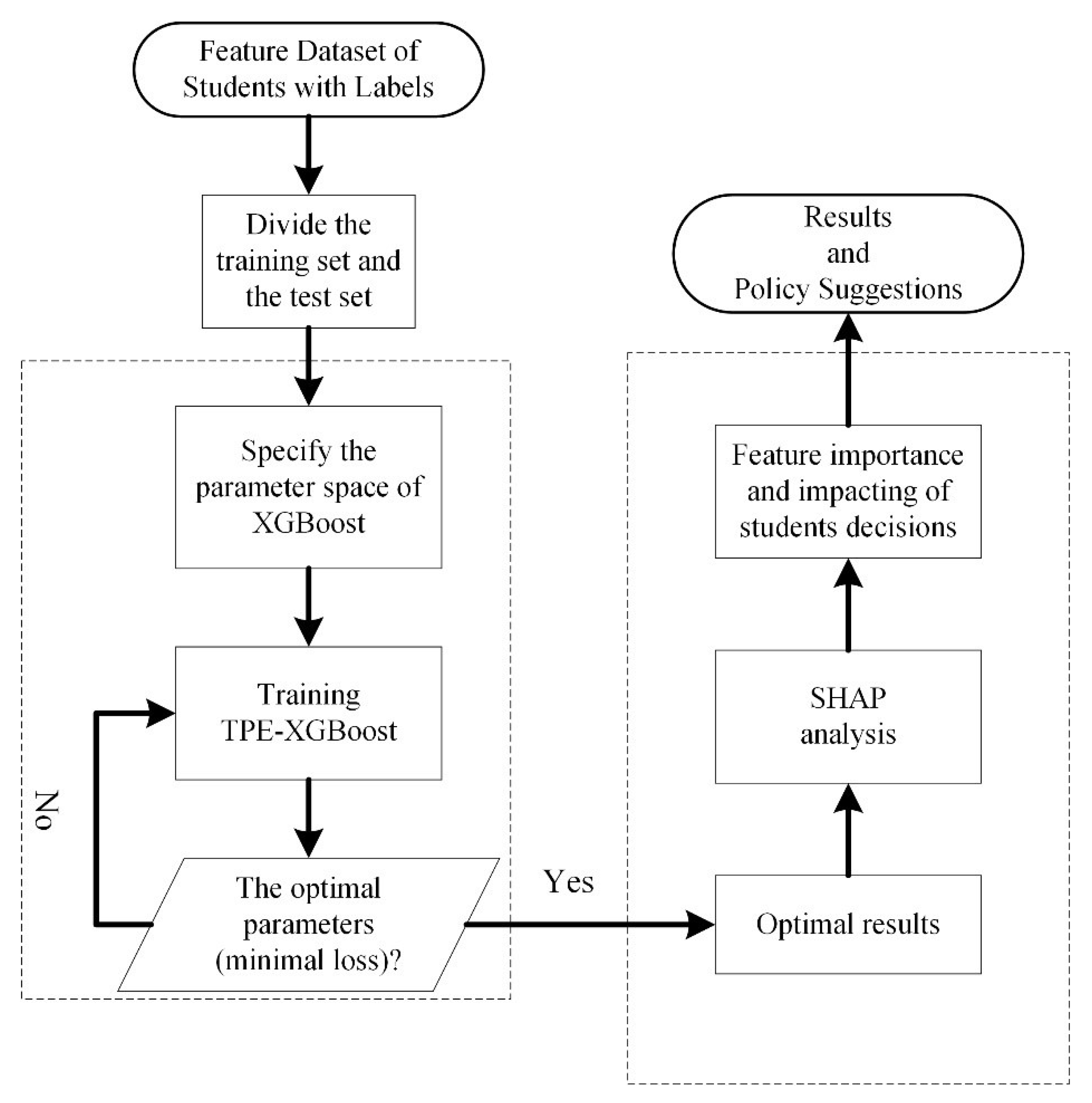
3. Materials and Methods

Figure 1 is the flow chart of methods used in this paper. We first collected the data and sorted it out to form a data set with students’ labels of choices and characteristics. Then, we used a hyperparametric optimization method called Tree-structured Parzen Estimator to obtain the optimal XGBoost model’s structure. Then, we further discussed the optimal predicted result to discover the factors that impact the students’ decisions. Specifically, the Shapley Additivity explanation method was employed to determine the impact of students’ basic information, academic characteristics, rewards, and honors on their decisions of final career choice. Finally, we summarized our research and put forward relevant policy suggestions.

3.1. XGBoost Algorithm

XGBoost, developed by Chen and Guestrin [24], is a powerful boosting algorithm that supports parallel computing. Recently, it has been utilized in various disciplines, such as energy forecasting [25,28] and the financial sector [26,29]. Its basic components are classification and regression trees (CARTs) and can be described as:

$$\widehat{y_i}={\displaystyle \sum }_{k=1}^K{f}_k\left(x_i\right), f_k\in F,$$

(1)

where $i=1,2,\dots ,n$. $n$ is number of samples, $F$ is the set of all CARTs in the model, and $fk$ is the function of $F$.

The objective function of XGBoost, as shown in Equation (2), is to minimize error term $L\left(\theta \right)$ and regularization item $\mathsf{\Omega }\left(\theta \right)$, which measures prediction error and complexity, respectively.

$$f_{obj}\left(\theta \right)=L\left(\theta \right)+\mathsf{\Omega }\left(\theta \right),$$

(2)

where $L\left(\theta \right)=l\left(y_i,\widehat{y_i}\right)={\displaystyle \sum }_{i=1}^n{\left(y_i-\widehat{y_i}\right)}^2, \mathsf{\Omega }\left(\theta \right)={\displaystyle \sum }_{k=1}^K\mathsf{\Omega }\left(f_k\right)$. That is, the first term is loss function, which evaluates the loss or error between the model’s predicted value and the true value. This function must be differentiable and convex; the second regularization term is used to control model complexity and tends to choose simple models to avoid over-fitting problems.

During the iterative training period, a new function f that does not affect the original model will be added in the time t to observe the objective function. If the newly added f can minimize the objective function as much as possible, it will be added, as shown in Equation (3).

$$f_{obj}{}^{\left(t\right)}={\displaystyle \sum }_{i=1}^n{\left(y_i-\left(\widehat{y_i}+f_t\left(x_i\right)\right)\right)}^2+\mathsf{\Omega }\left(f_t\right)+C,$$

(3)

where $f_t\left(x_i\right)$ denotes the newly added f in time t, and C is a constant term.

Next, we introduce the Taylor formula to expand the objective function $f_{obj}{}^{\left(t\right)}$ to achieve the purpose of approximation and simplification. The approximate objective function is shown as follows:

$$f_{obj}{}^{\left(t\right)}\approx {\displaystyle \sum }_{i=1}^n[l(y_i,{\widehat{y_i}}^{\left(t-1\right)})+g_i{f}_t\left(x_i\right)+\frac{1}{2}{h}_i{f}_i^2\left(x_i\right)]+\mathsf{\Omega }\left(f_t\right)+C,$$

(4)

where $g_i$ is the first step statistics of the loss function; $h_i$ is the second. $g_i={\partial }_{{\widehat{y}}^{\left(t-1\right)}}l(y_i,{\widehat{y}}^{\left(t-1\right)}), h_i={\partial }_{{\widehat{y}}^{\left(t-1\right)}}^{2}l(y_i,{\widehat{y}}^{\left(t-1\right)})$.

Suppose q represents tree structure, and w represents leaf weight; the compacity of model can be expressed as:

$$f_t\left(x\right)=w_{q\left(x\right)},w\in R^T,q:R^T\to \left\{1,2,\dots ,T\right\}.$$

(5)

Define the complexity as the sum of the number of leaves and squares of fraction value corresponding to leaf nodes in each tree, as shown in Equation (6):

$$\mathsf{\Omega }\left(f_t\right)=\gamma T+\frac{1}{2}\lambda {\displaystyle \sum }_{j=1}^T{w}_j^2,$$

(6)

where $\gamma ,\lambda$ are adjusted parameters to prevent over-fitting. Let $I_j=\left\{i\right|q\left(x_i\right)=j\}$ denote the set of leaf samples in the j-th tree, and $G_j={\displaystyle \sum }_{i\in I_j}{g}_i, H_j={\displaystyle \sum }_{i\in I_j}{h}_i$; we obtain:

$$f_{obj}{}^{\left(t\right)}={\displaystyle \sum }_{j=1}^T\left[G_j{w}_j+\frac{1}{2}\left(H_j+\lambda \right)w_j^2\right]+\gamma T.$$

(7)

Solve Equation (7); it is simple to obtain the following:

$$w_j^{*}=\frac{-G_j}{H_j+\lambda },$$

(8)

$$f_{obj}=-\frac{1}{2}{\displaystyle \sum }_{j=1}^T\frac{G_j}{H_j+\lambda }+\gamma T,$$

(9)

where $f_{obj}$ is a scoring function that measures the model performance. A smaller $f_{obj}$ means a better predictive model. The pseudocodes for split finding in XGBoost are shown in Algorithm 1:

Algorithm 1: Exact Greedy Algorithm for Split Finding

Input: $I$, instance set of current node

Input: $d,$ feature dimension

gain$\leftarrow$0

G$\leftarrow {\displaystyle \sum }_{i\in I}{g}_i,H\leftarrow {\displaystyle \sum }_{i\in I}{h}_i$

for$k=1$ to m do

$G_L\leftarrow 0$, $H_L\leftarrow 0$

for j in sorted (I, by $x_{jk}$) do

$G_L\leftarrow G_L+g_j,H_L\leftarrow H_L+h_j$

$G_R\leftarrow G-G_L,H_R\leftarrow H-H_L$

score$\leftarrow \max (score,\frac{G_L^2}{H_L+\lambda }+\frac{G_R^2}{H_R+\lambda }-\frac{G^2}{H+\lambda })$

end

end

Output: Split with max score

Thus, for CART algorithm, the computation complexity is $O\left(NMD\right)$, where $N$ is the number of samples, $M$ is the feature number, and $D$ denotes the depth of generated trees. When using CART as a base classifier, XGBoost explicitly adds regularization terms to control the complexity of the model, which helps prevent overfitting and thus improves the generalization of the model. Thus, the computation complexity of XGBoost is between $O\left(NlogN\right)$ and $O\left(log2k\right)$.

3.2. Tree-Structured Parzen Estimator for Model Optimization

Generally, hyperparameters refers to a set of parameters in which their values should be set before training starts (e.g., the number of CARTs and learning rate). They define the model architecture and control the learning process, playing a fundamental role in the development of machine learning models. Hyperparameter optimization is the process of adjusting hyperparameters to approximate the optimal prediction result. Compared with other methods (i.e., random search and grid search), automatic hyperparameter tuning can form the knowledge between parameters and models to reduce the number of tests and thus improve the efficiency of the tuning process. In this study, we implemented a variant of Bayesian optimization (BO), called Tree-structured Parzen Estimator, to automatically optimize the hyperparameters of the XGBoost model.

TPE converts superparameter space to a nonparametric density distribution to model the process of $p(x|y)$. There are three conversion modes: uniform distribution to truncated Gaussian mixture distribution, logarithmic uniform distribution to exponential-phase Gaussian mixture distribution, and discrete distribution to heavy-weighted discrete distribution. Then, the hyperparameter space is divided into two groups, namely good and bad samples, based on their fitness values and a predefined value $y^{*}$ (usually set to 15%), as described in Equation (10):

$$p\left(x|y\right)=\{\begin{array}{c}l\left(x\right),if y<y^{*}\\ g\left(x\right),if y\ge y^{*}\end{array},$$

(10)

where $l\left(x\right),g\left(x\right)$ represents the probabilities that the hyperparameter set $\left\{x^i\right\}$ is in the good and bad groups, respectively. Then, we can summarize expected improvement (EI) as:

$$E{I}_{y^{*}}\left(x\right)={{\displaystyle \int }}_{-\infty }^{\infty }\left(y^{*}-y\right)p\left(y|x\right)dy={{\displaystyle \int }}_{-\infty }^{y^{*}}\left(y^{*}-y\right)\frac{p(x|y)p\left(y\right)}{p\left(x\right)}dy.$$

(11)

At last, let $\gamma =p\left(y<y^{*}\right),$ and $p\left(x\right)={{\displaystyle \int }}^{ }p\left(x|y\right)p\left(y\right)dy=\gamma l\left(x\right)+\left(1-\gamma \right)g\left(x\right)$; we can thus easily obtain:

$$E{I}_{y^{*}}\left(x\right)={\left(r+\frac{g\left(x\right)}{l\left(x\right)}\left(1-\gamma \right)\right)}^{-1}.$$

(12)

Hence, each iteration returns an $x^{*}$ that obtains the maximum $EI$ value.

3.3. Shapley Additivity exPlanation

Model interpretability is the main challenge in the application of machine learning methods, but the field of educational big data prediction using machine learning has not been paid enough attention. In order to improve the interpretation of machine learning model, this paper uses the SHAP method to assign a value to each input variable to reflect its importance to the predictor [30].

For students’ feature subset $S\subseteq F$ (where F stands for the set of all factors), two models were trained to extract the effect of factor i. The first model $f_{S{\displaystyle \cup }\left\{i\right\}}(x_{S{\displaystyle \cup }\left\{i\right\}})$ was trained with factor I, while the other one $f_S\left(x_S\right)$ was trained without it, where $x_{S{\displaystyle \cup }\left\{i\right\}}$ and $x_S$ are the values of input features. Then, $f_{S{\displaystyle \cup }\left\{i\right\}}(x_{S{\displaystyle \cup }\left\{i\right\}})-f_S\left(x_S\right)$ was computed for each possible subset $S\subseteq F\backslash \left\{i\right\}.$ The Shapley value of a risk factor i is calculated using Equation (13).

$${\varphi }_i={\displaystyle \sum }_{S\subseteq F\backslash \left\{i\right\}}\frac{\left|S\right|!\left(\left|F\right|-\left|S\right|-1\right)!}{\left|F\right|!}(f_{S{\displaystyle \cup }\left\{i\right\}}\left(x_{S{\displaystyle \cup }\left\{i\right\}}\right)-f_S\left(x_S\right))$$

(13)

However, a major limitation of Equation (13) is that as the number of features increases, the computation cost will grow exponentially. To solve this problem, Lundberg et al. [20] proposed a computation-tractable explanation method, i.e., TreeExplainer, for decision tree-based ML models such as RF. The TreeExplainer method makes it much more efficient to calculate a risk factor’s SHAP value both locally and globally [31].

The SHAP combines optimal allocation with local explanations using the classic Shapley values. It would help users to trust the predictive models in not only what the prediction is but also why and how the prediction is made [32]. Thus, the SHAP interaction values can be calculated as the difference between the Shapley values of factor i with and without factor j in Equation (14):

$$\begin{gathered} {\varphi }_{i,j}={\displaystyle \sum }_{S\subseteq F\backslash \left\{i,j\right\}}\frac{\left|S\right|!\left(\left|F\right|-\left|S\right|-2\right)!}{\left|F\right|!}(f_{S{\displaystyle \cup }\left\{i,j\right\}}\left(x_{S{\displaystyle \cup }\left\{i,j\right\}}\right)-f_{S{\displaystyle \cup }\left\{i\right\}}\left(x_{S{\displaystyle \cup }\left\{i\right\}}\right) \\ -f_{S{\displaystyle \cup }\left\{j\right\}}\left(x_{S{\displaystyle \cup }\left\{j\right\}}\right)-f_S\left(x_S\right)). \end{gathered}$$

(14)

Based on this advantage, we can use it to explain the XGBoost model according to Decision Tree in order to find the impact of predicting student’ different characteristics on their final destination. Therefore, compared with existing methods (such as feature importance in Random Forests), SHAP can not only sort the feature importance but also show the positive and negative effects of features on the results so as to improve the interpretation ability of model output.

3.4. Data and Preprocess Methods

3.4.1. Data Source

This study obtained first-hand data through collection, investigation and other methods and conducted strict declassification at the beginning of data collection and integration. The data contain about 18,000 undergraduates in the class of 2018, 2019, and 2020 in a certain university, mainly including the initial data at the beginning of enrollment; students’ participation in scientific research, academic development, award, and excellence evaluation; the appointment of student leaders; student’ financial difficulties, loans, and repayment; student’ graduation status, etc. More details can be found in Appendix A.1. The data collected are changeable and traceable during their undergraduate period. Student behavior characteristics and growth patterns can be deeply mined through artificial intelligence methods such as data mining and association analysis.

3.4.2. Data Description

Based on the original data set, we further eliminated the data that are invalid and missing (see Appendix A.2). Finally, we secured a data set containing 10,292 students and 20 features, as shown in

Table 1. Dataset description.

	Classification	Description	Symbol
Input	Essential Data	Gender	X1
		National	X2
		Political Landscape	X3
		Examinee Category	X4
		Score of college entrance examination	X5
		Note	X6
		Category of students with difficulty	X7
	Honors	Scholarship awarded by university	X8
		Scholarship awarded by provincial	X9
		Total amount of money	X10
	GPA Data	GPA of First Term	X11
		GPA of Second Term	X12
		GPA of Third Term	X13
		GPA of Fourth Term	X14
		GPA of Fifth Term	X15
		GPA of Sixth Term	X16
		GPA of Seventh Term	X17
		GPA of Eighth Term	X18
		Overall GPA	X19
Output	Destination	Final Employment	Y

. Further graduation choices were divided finely into four categories, as shown in

Table 2. Breakdown of students’ graduation destination.

Classification	Content	Alphabetize	Population
Further Study in China	Master’s	Y1	4264
	Doctorate
	Preparing for the Entrance Exam
	Second Bachelor’s Degree
Employment	Sign Labor Contract	Y2	4372
	Sign an Employment Agreement
	Certificate of Employment
	Self-employed
	Freelance Work
	Joined the Army
	Volunteer in the West
Difficulties in Employment	Waiting for Employment in Beijing	Y3	617
	Return to Hometown for Employment
	Apply for Non-Employment
	Delay
Study Abroad	Has Gone Abroad	Y4	1038
	Plans to Go Abroad

.

4. Results and Discussion

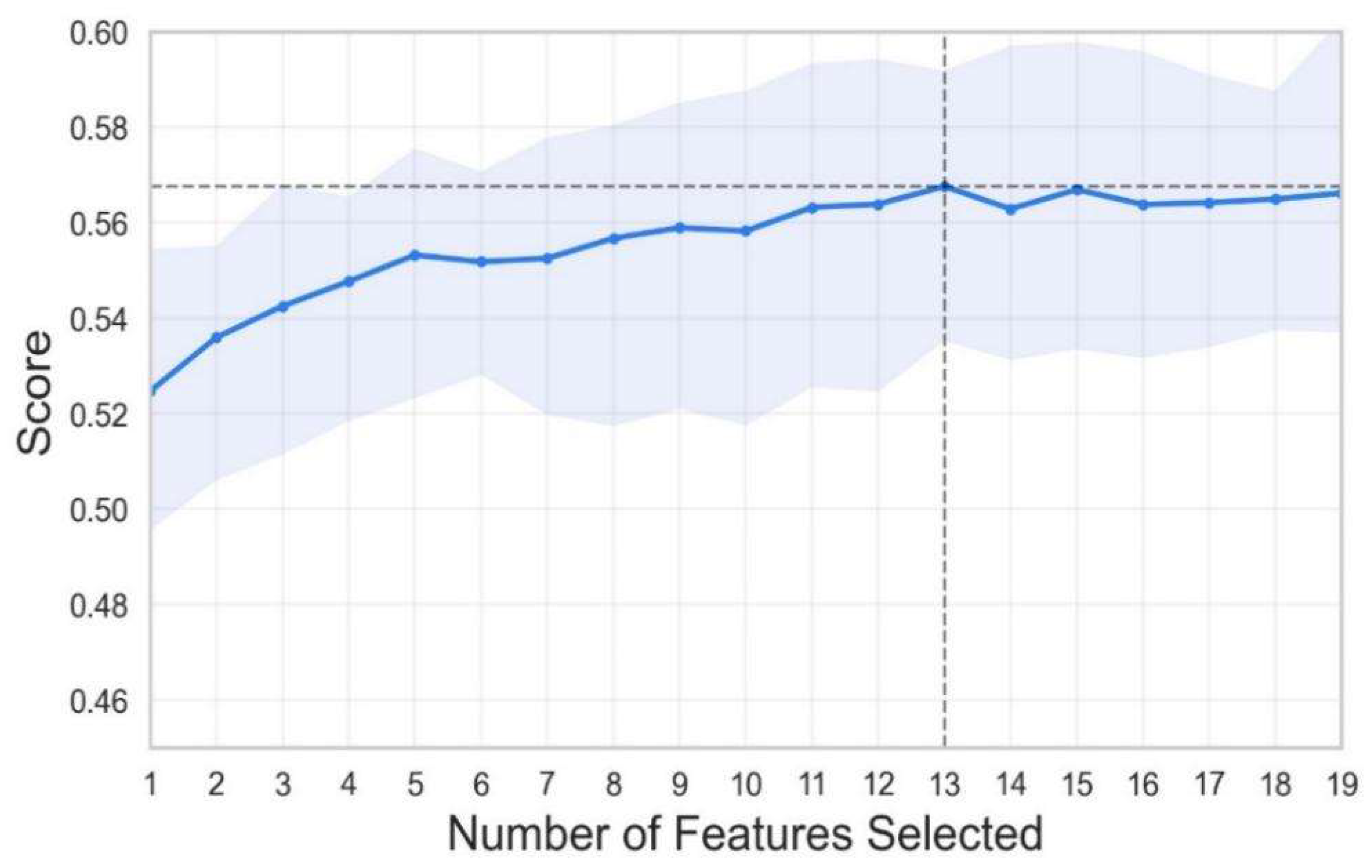
4.1. Feature Selection

In the machine learning method, it is easy to deal with highly correlated independent variables that may lead to over-fitting [33]. Therefore, detecting the correlation of related variables through correlation analysis is not that important. However, the variables (noise variables) that are not important to the model prediction results will not only increase the model redundancy, causing training interference, but are also not conducive to the interpretation of the model output. Hence, before starting model training, we first used Recursive Feature Elimination (RFE) for feature selection. RFE is a simple adverse selection method, which uses repeated multi-fold verification method to fit the model. See [34] for more details about RFE. Figure 2 illustrates the results of Recursive Feature Elimination in this paper.

As can be seen from Figure 2, when the input feature number is less than 13, the prediction score of the model increases along with the rising input features; when the parameter is higher than 13, with the increasing of input features, the prediction score of the model does not go up but down, indicating that noise variables have appeared in the model at this time. Therefore, we are sure that the optimal number of input variables of the model is 13. The best variable set is: X1, X4, X5, X7, X10, X11, X12, X14, X15, X16, X17, X18, X19.

4.2. Evaluation Metrics

On the basis of the above optimal variable set, the model was adjusted by TPE method by considering the importance of hyperparameters. Each type of sample was divided into four types: true positive (TP), false positive (FP), true negative (TN), and false negative (FN) according to the real category and prediction category of the sample. The F1-Score method is used to evaluate the model performance, as shown in Equation (15). The score of the final model is the average of F1 values of all categories. With the number of iterations set to 30, the parameter selection process is shown in Figure 2.

$$F1=\frac{2\times P\times R}{P+R},$$

(15)

where P denotes precision measuring the accuracy of the model, as shown in Equation (16); R is recall ratio representing the comprehensiveness of the model, as shown in Equation (17) [35,36]. Generally speaking, when the p-value is high, R value is usually low and vice versa. F1 value is proposed to comprehensively consider these two measurements and better indicate the prediction performance of the predictive model.

$$P=\frac{TP}{TP+FP}.$$

(16)

$$R=\frac{TP}{TP+FN}.$$

(17)

4.3. Comparison of Model’s Performance

In general, the larger the F1 value of the model, the better the prediction performance of the model. On the contrary, the smaller the F1 value is, it indicates that the constructed model cannot well adapt to the research problem in this paper. We need to consider rebuilding the feature input or change a more suitable model. In the following section, we further conduct 10-fold cross validation and paired t-test [37] to compare our model with other mainstream methods.

As shown in Figure 3, the best F1 value in hyperparameter optimization process is 0.872, showing that the model constructed in this paper can better predict the decisions of college students. The combination of hyperparameters corresponding to the optimal F1 value is shown in

Table 3. Hyper-parameters of XGBoost.

Hyperparameters	Value	Meaning
n_estimators	331	Number of trees
subsample	0.4494	Percentage of random sample
max_depth	10	Maximum depth of each tree
colsample_bytree	0.5294	Random sampling characteristics
gamma	3	Penalty term for complexity
learning_rate	0.1533	Learning rate

. In addition, to provide more numerical insights, we compared the proposed method with the state-of-the-art methods [38], as shown in

Table 4. Comparisons of proposed method with other mainstream methods (10-fold average).

Model	p	R	F1	Performance Comparison (%)
Decision Tree	0.803	0.812	0.807	−7.454% ** (0.035)
SVM	0.791	0.788	0.789	−9.518% * (0.072)
Random Forest	0.847	0.824	0.835	−4.243% *** (0.001)
Light GBM	0.889	0.846	0.866	−0.689% (0.301)
XGBoost	0.891	0.854	0.872	/

Note: XGBoost is the benchmark for paired t-test. Negative performance of F1 indicates that the method presents worse performance than XGBoost. * At the 10% level. ** At the 5% level. *** At the 1% level. p-Values are in parentheses.

.

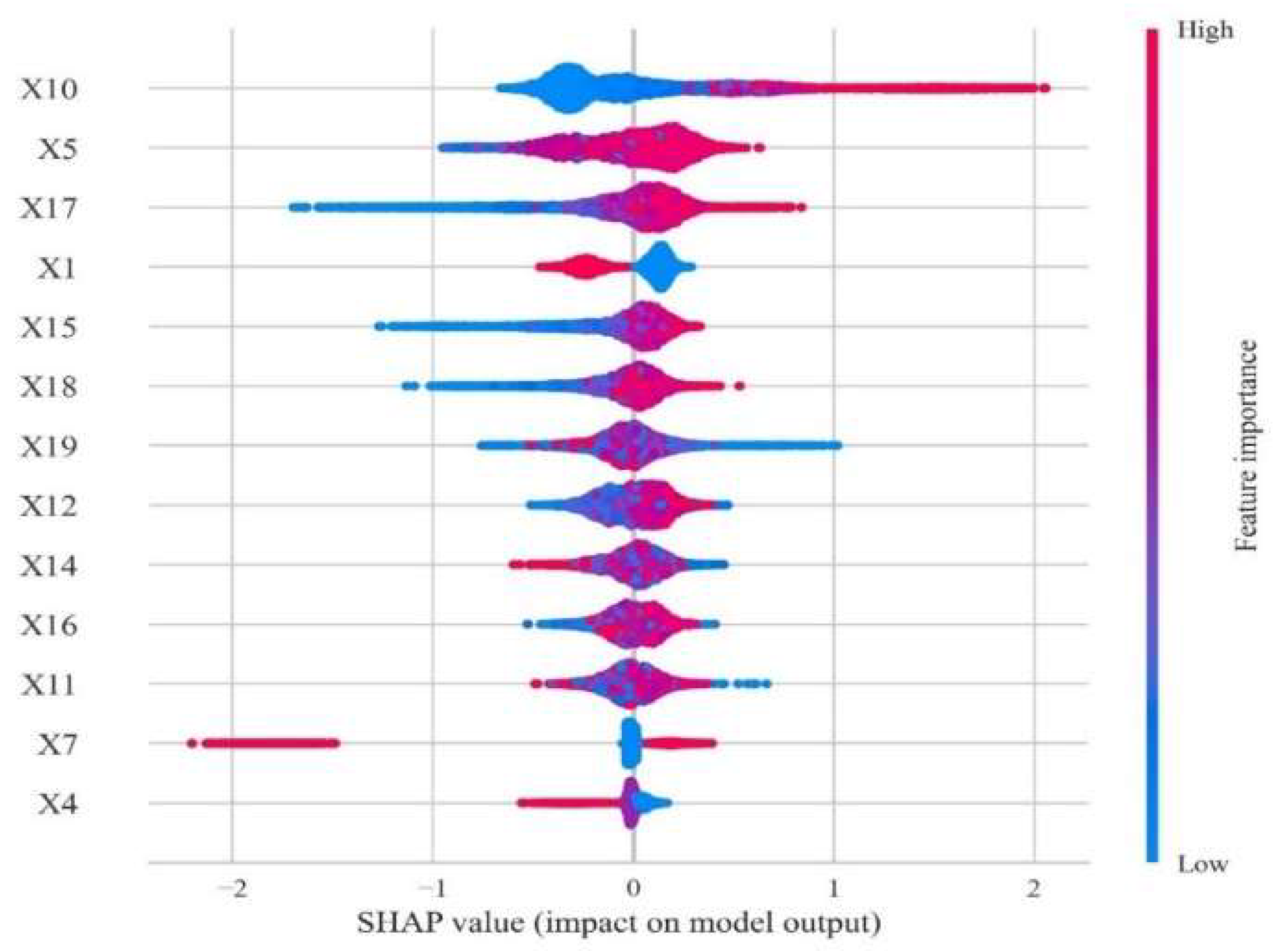
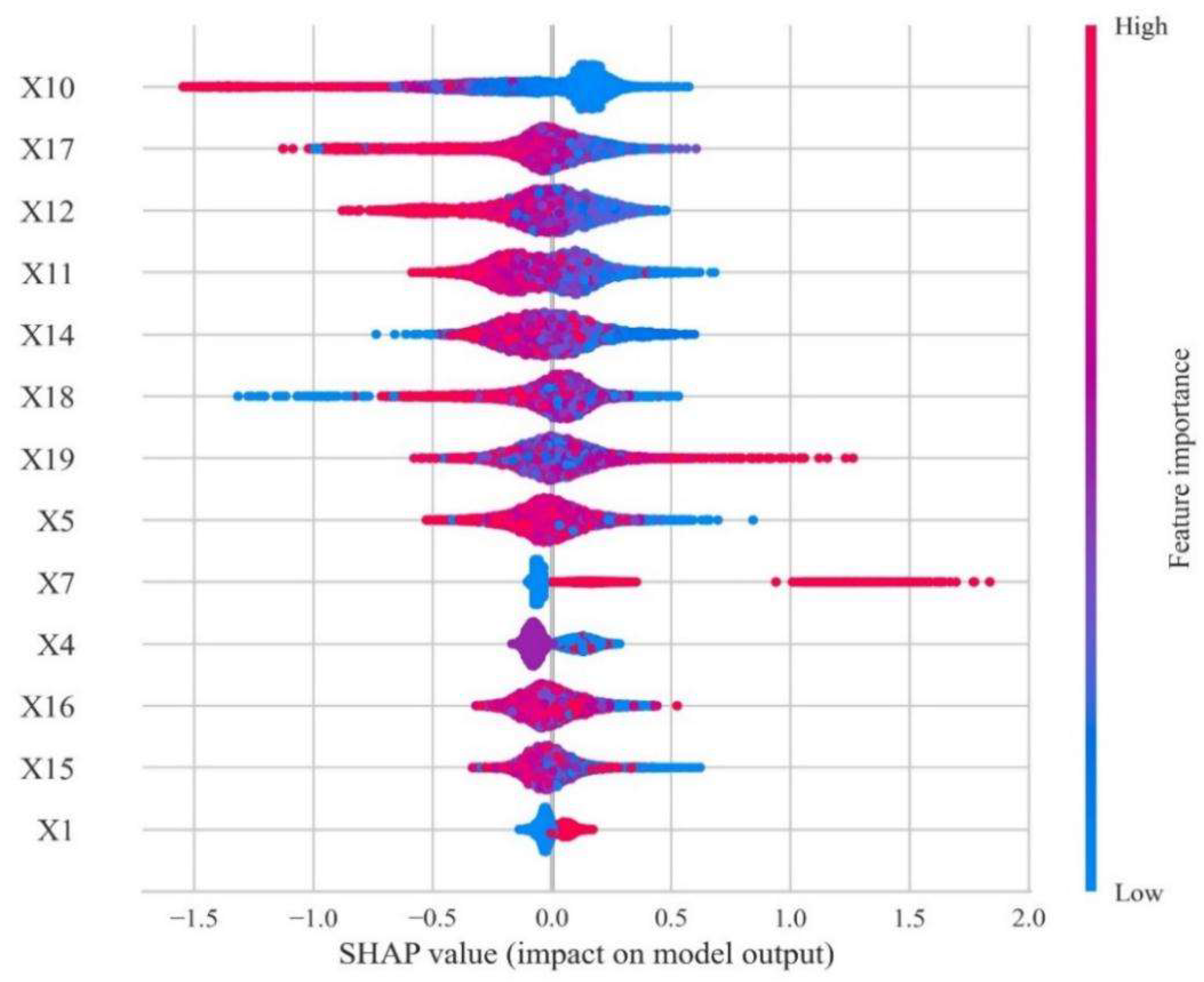
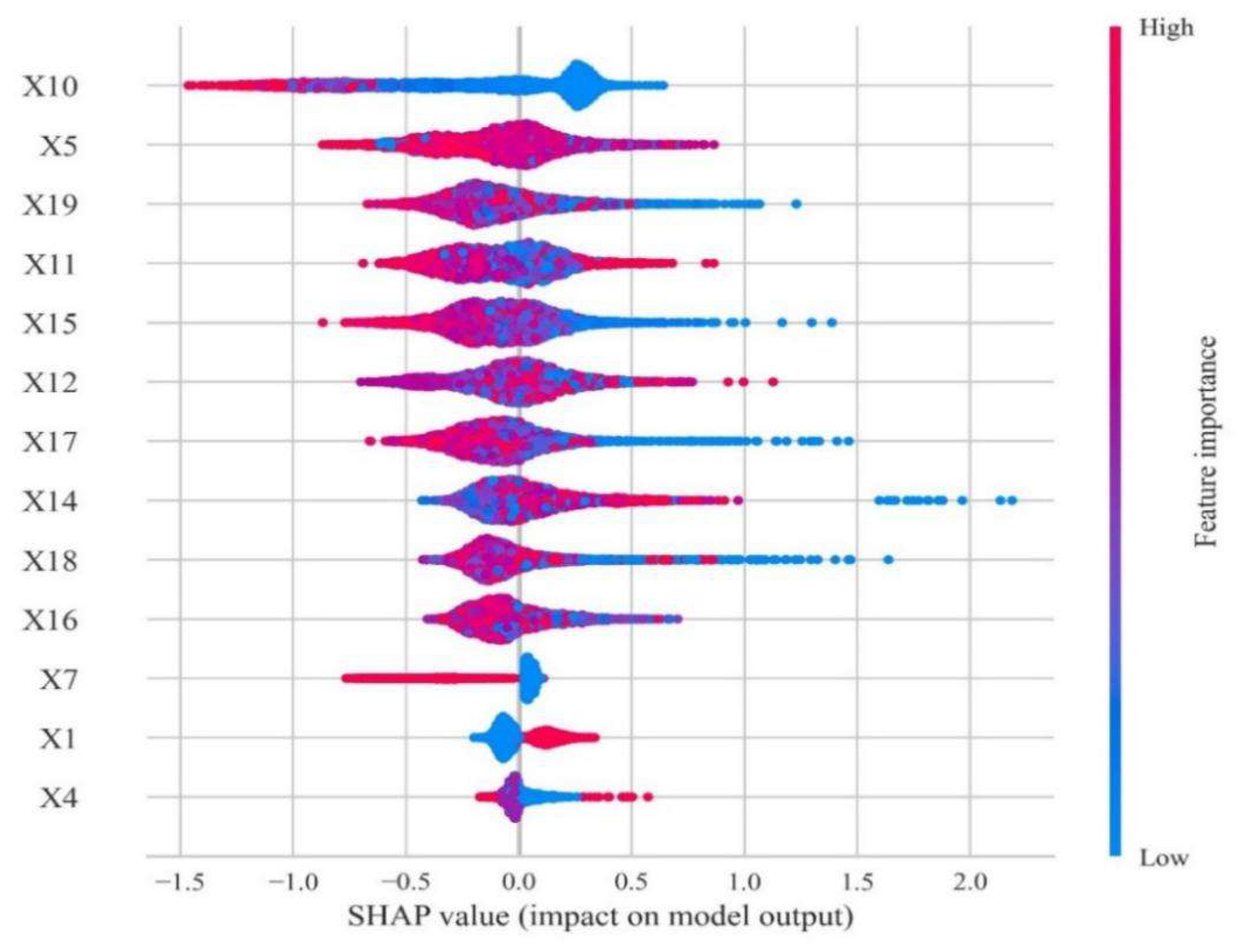
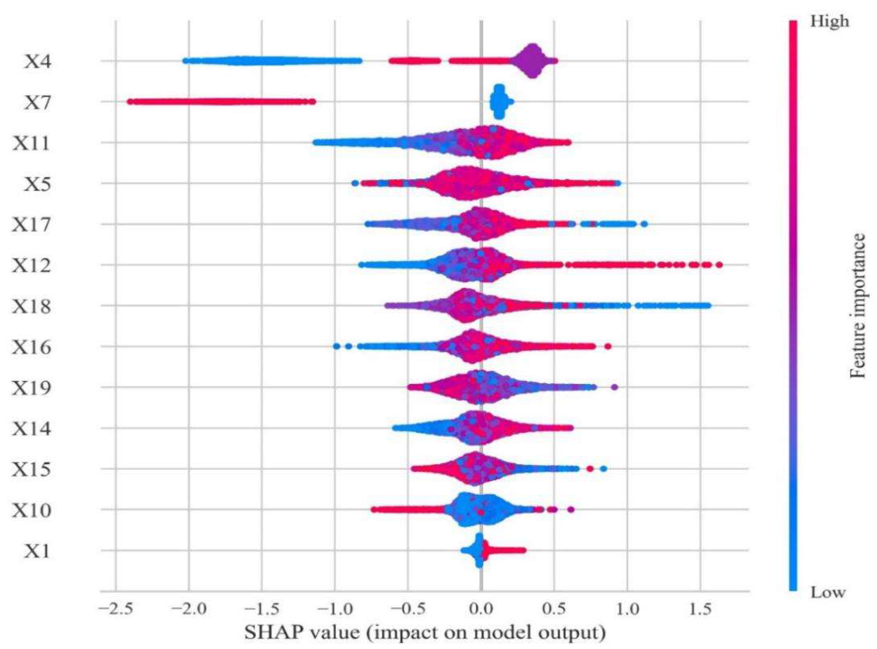
4.4. SHAP Approach for Results Interpretation

Under the structure of the optimal model above, the SHAP summary diagram is used in this section to explain the overall prediction results of the model. This paper explains the model of students studying in China, at work, under difficult circumstance, and studying overseas, respectively, so as to explore the predictive role of different characteristics in the final direction of students.

Choose to study in China: students studying in China account for a large proportion of the students studied, and the output of their prediction results is shown in Figure 4.

In Figure 4, the closer the color of sample points to red, the larger the value of sample points it shows and vice versa. For those students, features X10, X5, X17, X1, and X15 are the five most important variables for prediction, i.e., total amount of scholarship, college entrance examination score, GPA of the seventh semester, gender, and GPA of the fifth semester. Among them, in terms of X10, the red sample points are mainly distributed in the positive area, suggesting that the larger the total amount of scholarships, the higher the SHAP value of the model, indicating that students with more scholarships tend to choose domestic education.

For X5, although a small number of red sample points are distributed in the negative area of SHAP, most of the red sample points are distributed near the positive area of SHAP, showcasing that students with high grades in college entrance examination also tend to study in China; the grade points of the seventh semester (X17) and the fifth semester (X15) are the same, and the red sample points tend to be distributed in the area with positive SHAP value, indicating that students with higher eigenvalues also tend to choose domestic education. Interestingly, in terms of gender (X1), the red dots (i.e., females) are mainly distributed in the negative area of SHAP, while the blue dots (males) are mostly distributed in the positive area of SHAP, suggesting that boys in school are more likely to choose domestic education than girls.

Choose to work: According to Figure 5, we can see that for students who are predicted to work, the features X10, X17, X12, X11, and X14 are the five most important variables for the prediction, which are the total amount of scholarships, GPA in the seventh semester, GPA in the second semester, GPA in the first semester, and GPA in the fourth semester. By analyzing feature X10, it is found that most of the red sample points are distributed in the area with negative SHAP value, indicating that the more scholarship students win, the less they will choose to work, which is consistent with the analysis above, which is to say that students who win more scholarships prefer to study in China. The remaining four variables are academic variables, and most of the blue dots are distributed in the area where the SHAP value is positive, showing that students with unremarkableGPA in the seventh, second, first, and fourth semester will prefer to work.

Difficult to find a job: from Figure 6, we can see that for students whose decisions are hard to predict, the features X10, X5, X19, X11, and X15 are the five most important variables for prediction, which equal to the total amount of scholarships, score of college entrance examination, average GPA during college, GPA in the first semester, and GPA in the fifth semester.

By analyzing the feature X10, we can find that most of the red sample points are distributed in the area with negative SHAP value, indicating that the more scholarships students win, the less they will be distributed in this category; that is, students who obtain more scholarships generally will not face the pressure of delayed graduation or employment difficulties. It is worth noting that the second variable that is more important for prediction is the score of college entrance examination (X5). In terms of analyzing this score, it can be found that the red sample points are distributed in both areas where the SHAP value is positive and negative, but the higher scores (shown as red sample points) are generally distributed in the areas where the SHAP value is negative, and the general scores (color near purple) are more distributed in the areas where the SHAP value is positive. It demonstrates that students with high grades tend to maintain excellent learning habits and will not face the problems of delayed graduation or employment difficulties during college years or graduation, while students with medium grades have a certain probability of facing the above problems. The remaining three variables are academic variables, and most of the blue dots are distributed in the area with positive SHAP value, indicating that students with poor academic performance often face certain employment and graduation difficulties.

Choose to study aboard: according to Figure 7, for the prediction of students studying abroad, feature X4, X7, X11, X5, and X17 are the five most crucial variables for the prediction, i.e., category of exam taker, category of difficult student, GPA in the first semester, score of college entrance examination, and GPA in the seventh semester. By analyzing feature X4, it is found that most of the blue dot (i.e., students in rural areas) students are distributed in the negative area of SHAP, indicating that most of these students will not choose to study abroad. For feature X7, the category of students with difficulties (family difficulties, family difficulties, and disabilities), samples with large numbers are mostly distributed in areas with negative number of SHAP, indicating that most students with difficulties will not choose to study abroad. Compared with other students, those in rural areas and students with difficulties are not able to afford to go abroad, so they are not likely to study abroad. The finding above is consistent with the actual situation. For feature X11, we may find that most of blue points are distributed in the area with negative value of SHAP, indicating that low GPA in the first semester will have negative effect on their intention of studying abroad. The features X5 and X17 are less obvious, which means that the score of college entrance examination and GPA in the seventh semester have little impact on studying abroad.

5. Conclusions

In this study, we used machine learning tools such as XGBoost, TPE, and SHAP to perform prediction of college students’ career choice. The methods are supported by using data from one college located in Beijing. Based on the analysis above, we may draw the following conclusions:

(1)

Within students’ basic information, the score of college entrance examination plays an important role in predicting graduates’ career choice. The results of empirical analysis show that students with high scores tend to choose further education in China, and the higher their scores, the less likely they are to face employment and graduation problems. However, it is worth noting that more students with an intermediate score suffer in employment and graduation compared with those students achieving low scores.

(2)

Total amount of scholarships has an important impact on the final academic direction. Students with a higher amount tend to choose domestic postgraduate education rather than employment because they have better learning ability and make clear academic plans. At the same time, it should be noted that the evaluation of scholarship is based on the comprehensive achievements rather than GPA solely, so it is necessary to remind students of the importance of comprehensive development in their lower grade.

(3)

In terms of academic data, GPA in the first semester has a vital impact on students’ future choice, which is quite obvious among students taking up further education. Most students with low GPA in the first semester will not consider studying abroad or further education in China. Most of them go to job market directly, or some of them face problems in employment or graduation.

Limitations and Future Directions

The limitations of this work could be the heterogeneity of the dataset and its quantity, such as the lack of more detailed personal characteristics (e.g., the education level of their parents). Future studies should undertake surveys to collect more data of different schools and more personal characteristics to supplement or verify the algorithm. Thus, the ML algorithm for predicting students’ career choice can be updated and re-trained to achieve more reliable and accurate results.

References

1. Jordan, M.I.; Mitchell, T.M. Machine learning: Trends, perspectives, and prospects. Science 2008, 349, 255–260. [Google Scholar] [CrossRef] [PubMed]
2. Olaya, D.; Vásquez, J.; Maldonado, S.; Miranda, J.; Verbeke, W. Uplift Modeling for preventing student dropout in higher education. Decis. Support Syst. 2020, 134, 113320. [Google Scholar] [CrossRef]
3. Maldonado, S.; Miranda, J.; Olaya, D.; Vásquez, J.; Verbeke, W. Redefining profit metrics for boosting student retention in higher education. Decis. Support Syst. 2021, 143, 113493. [Google Scholar] [CrossRef]
4. Nauman, M.; Akhtar, N.; Alhudhaif, A.; Alothaim, A. Guaranteeing correctness of machine learning based decision making at higher educational institutions. IEEE Access 2021, 9, 92864–92880. [Google Scholar] [CrossRef]
5. Erikson, E.H. Identity: Youth and Crisis; WW Norton & Company: Manhattan, NY, USA, 1994; pp. 176–200. [Google Scholar]
6. Marcia, J.E.; Waterman, A.S.; Matteson, D.R.; Archer, S.L. Ego Identity: A Handbook for Psychosocial Research; Springer Science and Business Media: New York, NY, USA, 2012. [Google Scholar]
7. Chrysafiadi, K.; Virvou, M. Student modeling approaches: A literature review for the last decade. Expert Syst. Appl. 2013, 40, 4715–4729. [Google Scholar] [CrossRef]
8. Wan, S.; Niu, Z. An e-learning recommendation approach based on the self-organization of learning resource. Knowl.-Based Syst. 2018, 160, 71–87. [Google Scholar] [CrossRef]
9. Hsia, T.C.; Shie, A.J.; Chen, L.C. Course planning of extension education to meet market demand by using data mining techniques—An example of Chinkuo technology university in Taiwan. Expert Syst. Appl. 2008, 34, 596–602. [Google Scholar] [CrossRef]
10. Injadat, M.; Moubayed, A.; Nassif, A.B.; Shami, A. Systematic ensemble model selection approach for educational data mining. Knowl.-Based Syst. 2020, 200, 105992. [Google Scholar] [CrossRef]
11. Alam, T.M.; Shaukat, K.; Hameed, I.A.; Khan, W.A.; Sarwar, M.U.; Iqbal, F.; Luo, S. A novel framework for prognostic factors identification of malignant mesothelioma through association rule mining. Biomed. Signal Process. Control 2021, 68, 102726. [Google Scholar] [CrossRef]
12. Shuhidan, S.M.; Nori, W.M. Accounting information system and decision useful information fit towards cost conscious strategy in Malaysian higher education institutions. Procedia Econ. Financ. 2015, 31, 885–895. [Google Scholar] [CrossRef]
13. Noaman, A.Y.; Ahmed, F.F. ERP systems functionalities in higher education. Procedia Comput. Sci. 2015, 65, 385–395. [Google Scholar] [CrossRef] [Green Version]
14. Wen, Z.; Qiang, W.; Ye, Y.; Yoshida, T. A 2020 perspective on “DeRec: A data-driven approach to accurate recommendation with deep learning and weighted loss function”. Electron. Commer. Res. Appl. 2021, 48, 101064. [Google Scholar]
15. Anastasios, T.; Cleo, S.; Effie, P.; Olivier, T.; George, M. Institutional research management using an integrated information system. Procedia-Soc. Behav. Sci. 2013, 73, 518–525. [Google Scholar] [CrossRef]
16. Wen, Z.; Shaoshan, Y.; Jian, L.; Xin, T.; Yoshida, T. Credit risk prediction of SMEs in supply chain finance by fusing demographic and behavioral data. Transp. Res. Part E, 2022; in press. [Google Scholar]
17. Wen, Z.; Wang, Q.; Yoshida, T.; Jian, L. RP-LGMC: Rating prediction based on local and global information with matrix clustering. Comput. Oper. Res. 2021, 129, 105228. [Google Scholar]
18. Wen, Z.; Li, X.; Li, J.; Yang, Y. Two-stage Rating Prediction Approach Based on Matrix Clustering on Implicit Information. IEEE Trans. Comput. Soc. Syst. 2020, 7, 517–535. [Google Scholar]
19. Shaukat, K.; Nawaz, I.; Aslam, S.; Zaheer, S.; Shaukat, U. Student’s performance in the context of data mining. In Proceedings of the 2016 19th International Multi-Topic Conference (INMIC), Islamabad, Pakistan, 1–8 December 2016; IEEE: Piscataway, NJ, USA, 2016. [Google Scholar]
20. Shaukat, K.; Nawaz, I.; Aslam, S.; Zaheer, S.; Shaukat, U. Student’s Performance: A Data Mining Perspective; LAP Lambert Academic Publishing: Saarbrücken, Germany, 2017. [Google Scholar]
21. Alam, T.M.; Mushtaq, M.; Shaukat, K.; Hameed, I.A.; Sarwar, M.U.; Luo, S. A Novel Method for Performance Measurement of Public Educational Institutions Using Machine Learning Models. Appl. Sci. 2021, 11, 9296. [Google Scholar] [CrossRef]
22. Amez, S.; Baert, S. Smartphone use and academic performance: A literature review. Int. J. Educ. Res. 2020, 103, 101618. [Google Scholar] [CrossRef]
23. Nieto, Y.; Gacía-Díaz, V.; Montenegro, C.; González, C.C.; Crespo, R.G. Usage of machine learning for strategic decision making at higher educational institutions. IEEE Access 2019, 7, 75007–75017. [Google Scholar] [CrossRef]
24. Chen, T.; Guestrin, C. Xgboost: A scalable tree boosting system. In Proceedings of the 22nd ACM Sigkdd International Conference on Knowledge Discovery and Data Mining, San Francisco, CA, USA, 24–27 August 2016; pp. 785–794. [Google Scholar]
25. Yang, L.; Zhao, Y.; Niu, X.; Song, Z.; Gao, Q.; Wu, J. Municipal Solid Waste Forecasting in China Based on Machine Learning Models. Front. Energy Res. 2021, 9, 763977. [Google Scholar] [CrossRef]
26. Jabeur, S.B.; Mefteh-Wali, S.; Viviani, J.L. Forecasting gold price with the XGBoost algorithm and SHAP interaction values. Ann. Oper. Res. 2021, 1–21. [Google Scholar] [CrossRef]
27. Varshney, K.R.; Alemzadeh, H. On the safety of machine learning: Cyber-physical systems, decision sciences, and data products. Big Data 2017, 5, 246–255. [Google Scholar] [CrossRef] [PubMed]
28. De Clercq, D.; Wen, Z.; Fei, F.; Caicedo, L.; Yuan, K.; Shang, R. Interpretable machine learning for predicting biomethane production in industrial-scale anaerobic co-digestion. Sci. Total Environ. 2020, 712, 134574. [Google Scholar] [CrossRef] [PubMed]
29. Jiang, C.; Wang, Z.; Zhao, H. A prediction-driven mixture cure model and its application in credit scoring. Eur. J. Oper. Res. 2019, 277, 20–31. [Google Scholar] [CrossRef]
30. Lundberg, S.M.; Lee, S.I. A unified approach to interpreting model predictions. In Proceedings of the 31st International Conference on Neural Information Processing Systems 2017, Los Angeles, CA, USA, 4–7 December 2017; pp. 4768–4777. [Google Scholar]
31. Lundberg, S.M.; Erion, G.; Chen, H.; DeGrave, A.; Prutkin, J.M.; Nair, B.; Lee, S.I. From local explanations to global understanding with explainable AI for trees. Nat. Mach. Intell. 2020, 2, 56–67. [Google Scholar] [CrossRef]
32. Ayoub, J.; Yang, X.J.; Zhou, F. Combat COVID-19 infodemic using explainable natural language processing models. Inf. Processing Manag. 2021, 58, 102569. [Google Scholar] [CrossRef]
33. Shaukat, K.; Luo, S.; Varadharajan, V.; Hameed, I.A.; Xu, M. A survey on machine learning techniques for cyber security in the last decade. IEEE Access 2020, 8, 222310–222354. [Google Scholar] [CrossRef]
34. Shieh, M.D.; Yang, C.C. Multiclass SVM-RFE for product form feature selection. Expert Syst. Appl. 2008, 35, 531–541. [Google Scholar] [CrossRef]
35. Shaukat, K.; Luo, S.; Varadharajan, V.; Hameed, I.A.; Chen, S.; Liu, D.; Li, J. Performance comparison and current challenges of using machine learning techniques in cybersecurity. Energies 2020, 13, 2509. [Google Scholar] [CrossRef]
36. Shaukat, K.; Luo, S.; Chen, S.; Liu, D. Cyber threat detection using machine learning techniques: A performance evaluation perspective. In Proceedings of the 2020 International Conference on Cyber Warfare and Security (ICCWS), Norfolk, VA, USA, 1–6 October 2020; IEEE: Piscataway, NJ, USA, 2020. [Google Scholar]
37. Kim, T.K. T-test as a parametric statistic. Korean J. Anesthesiol. 2015, 68, 540. [Google Scholar] [CrossRef] [Green Version]
38. Nie, M.; Xiong, Z.; Zhong, R.; Deng, W.; Yang, G. Career Choice Prediction Based on Campus Big Data—Mining the Potential Behavior of College Students. Appl. Sci. 2020, 10, 2841. [Google Scholar] [CrossRef] [Green Version]
Figure 1. Research Framework.
Mathematics 10 01289 g001
Figure 2. RFE feature selection results of XGBoost.
Mathematics 10 01289 g002
Figure 3. TPE optimization process.
Mathematics 10 01289 g003
Figure 4. SHAP summary diagram of domestic advanced students.
Mathematics 10 01289 g004
Figure 5. SHAP summary diagram of successful employment students.
Mathematics 10 01289 g005
Figure 6. SHAP summary diagram of difficult students.
Mathematics 10 01289 g006
Figure 7. SHAP summary diagram of students studying abroad.
Mathematics 10 01289 g007