
Third-Order Superharmonic Resonance Analysis and Control in a Nonlinear Dynamical System

 ,
,  , , and
Abstract
:1. Introduction
2. Third-Order Superharmonic Resonance Analysis
3. Superharmonic Resonance Curves and Discussion
4. Concluding Remarks
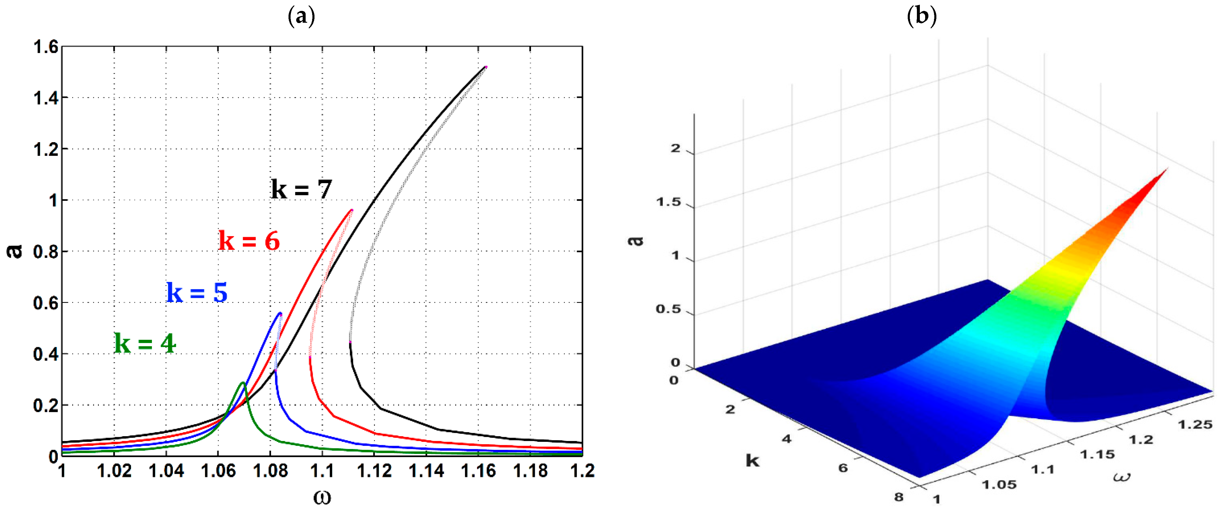
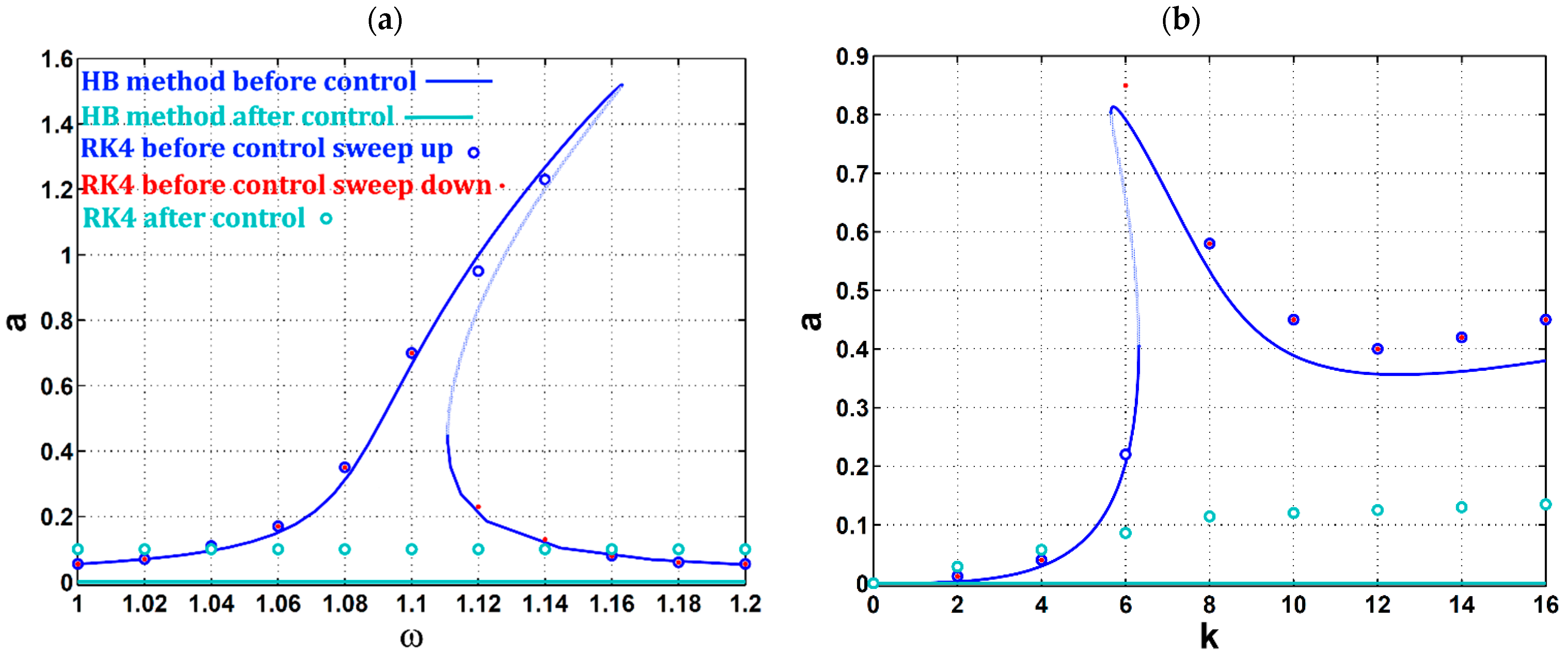
- The greater the excitation amplitude was, the more the frequency response curves rose and bent to the right with a slight right shift of the whole curve due to the domination of the cubic nonlinearity.
- The unstable solutions paths extended proportionally, with leading to a more severe jump from the curve’s peak to the lower values on the same curve.
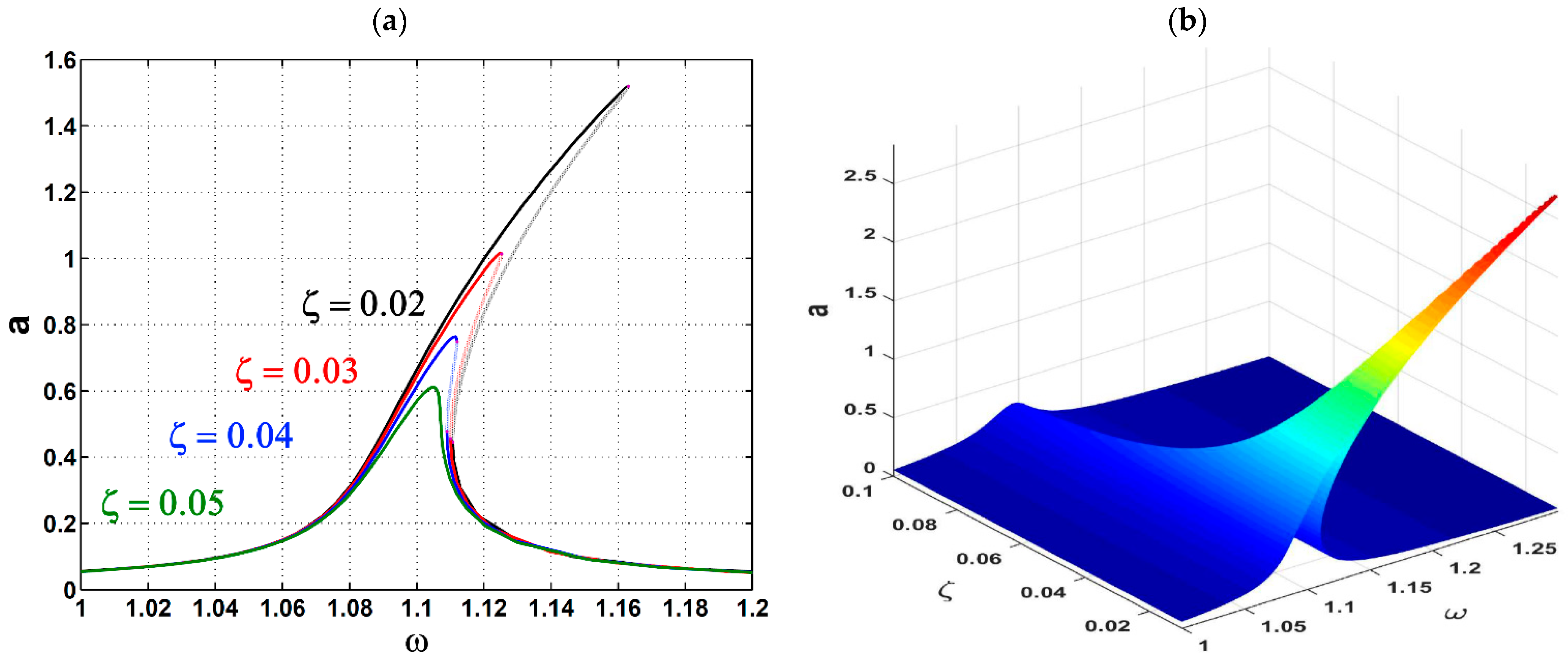
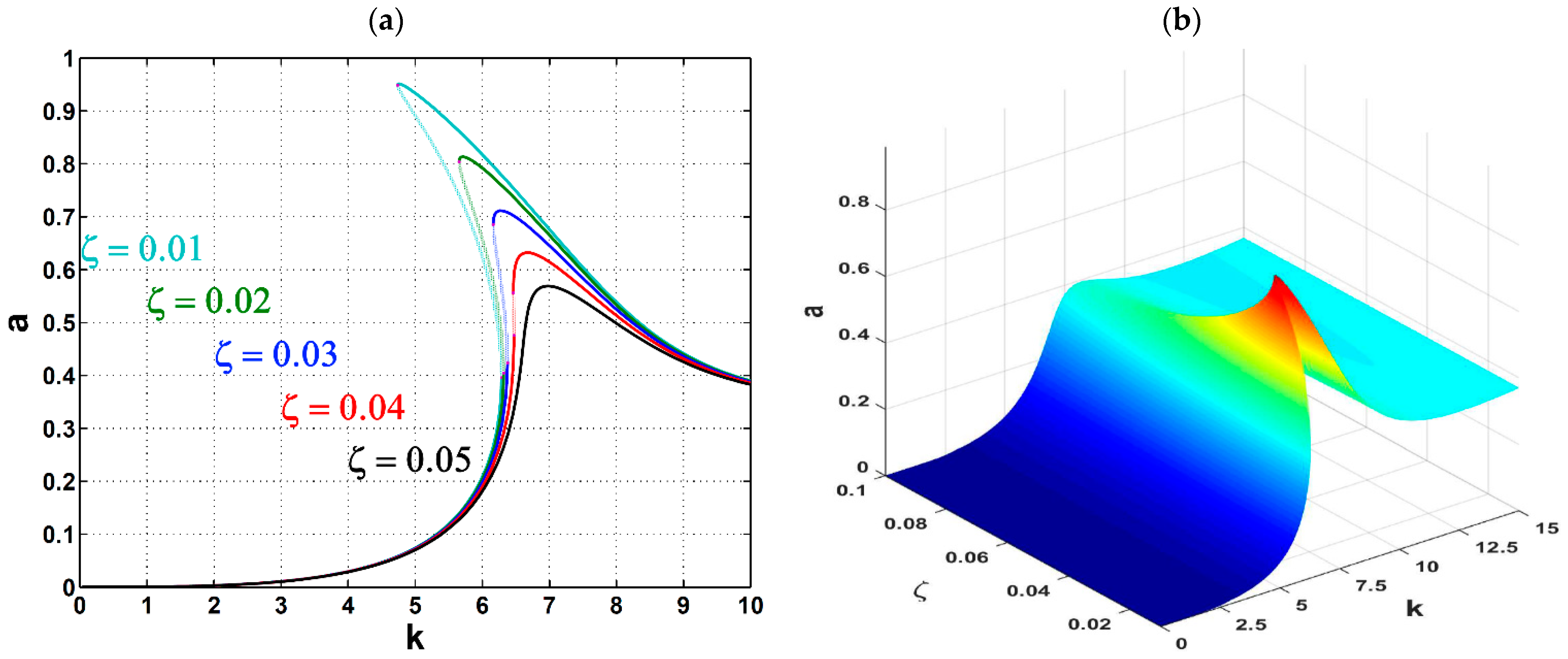
- The damping coefficient could help in suppressing the curve’s peak that led to a shorter unstable path and a lower possibility of encountering jumps along the curve.
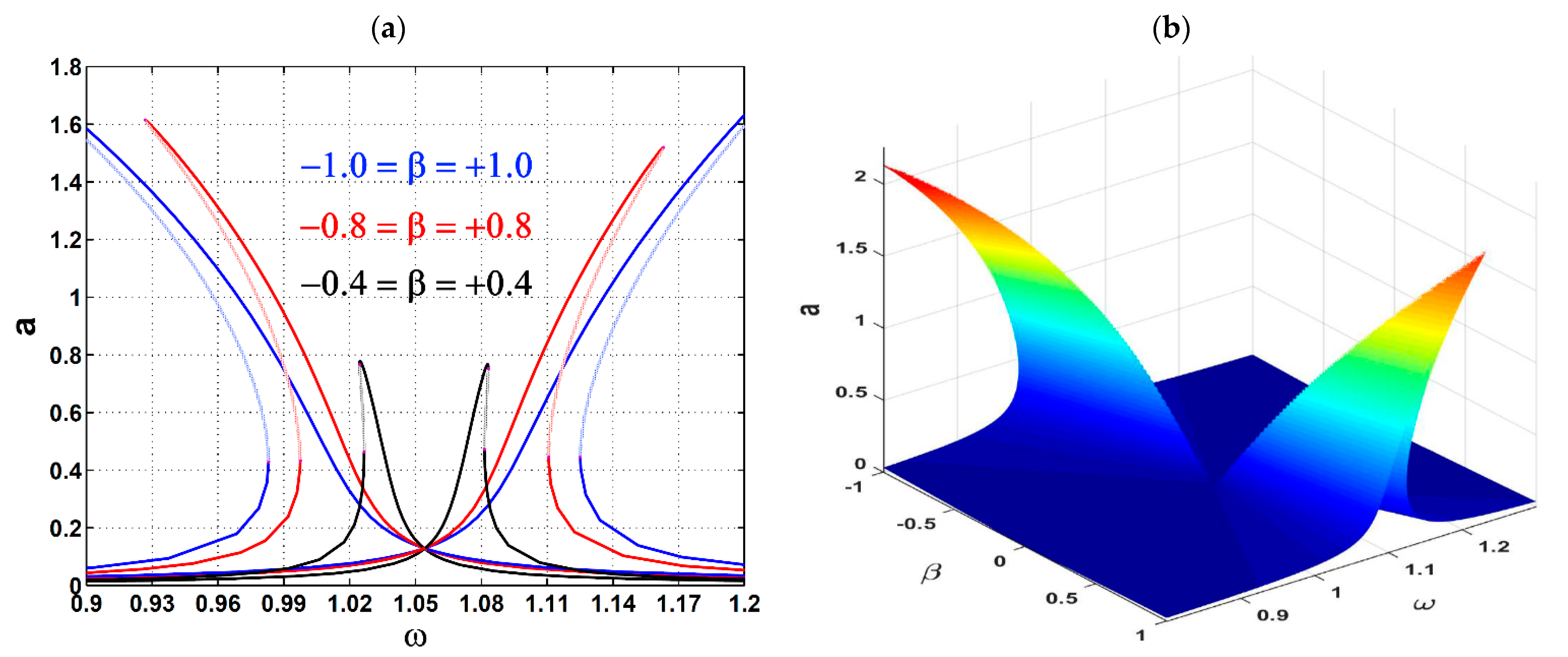
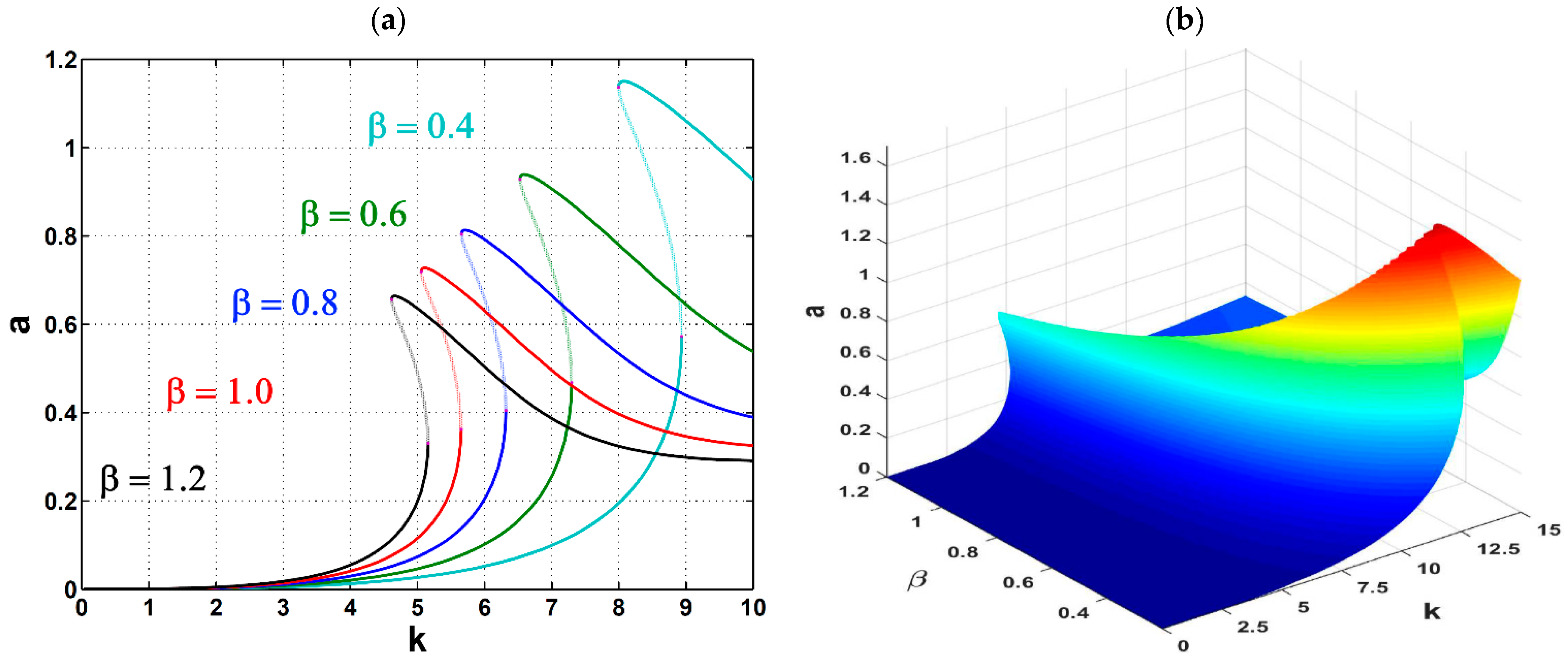
- Raising the value of the cubic-nonlinearity coefficient positively (or negatively) forced the curve to bend more to the right (or to the left) due to the hardening-type (or the softening-type) spring.
- The lower the value of , the lower the curve’s peak became.
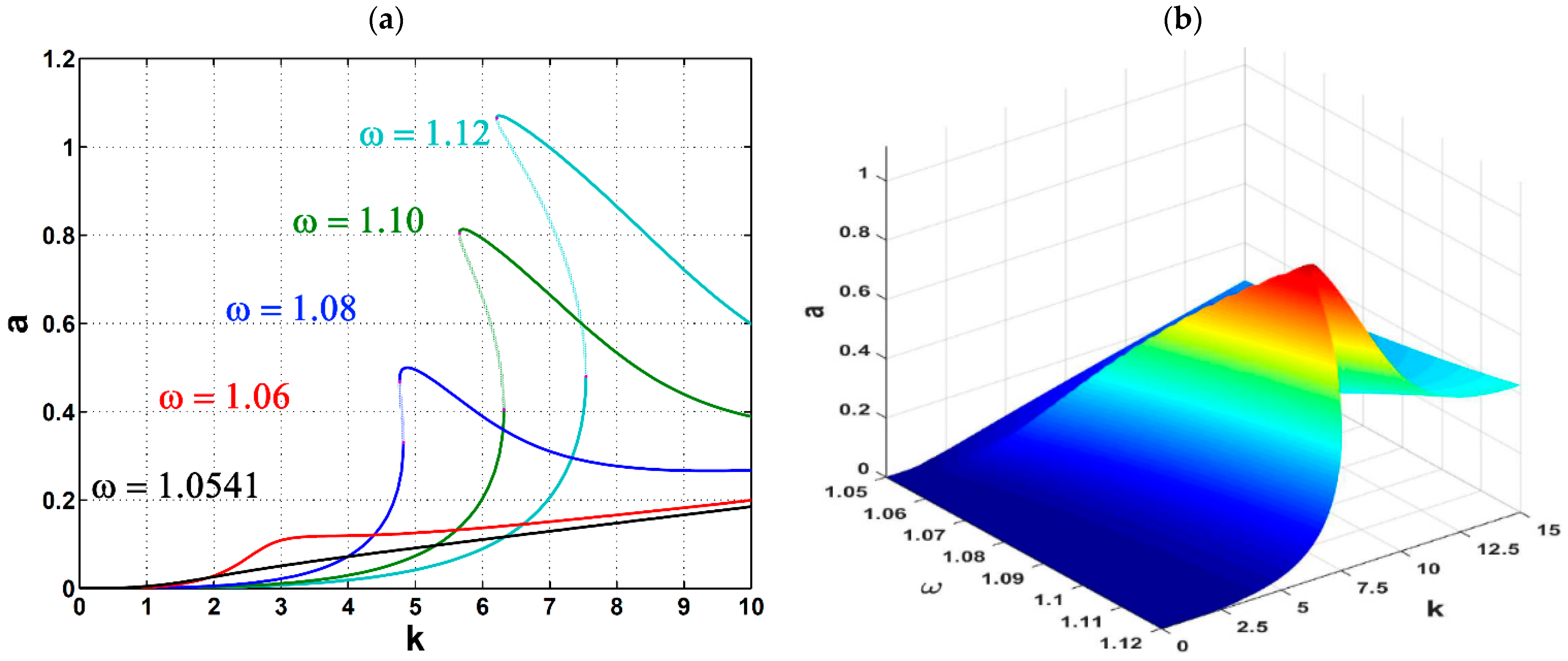
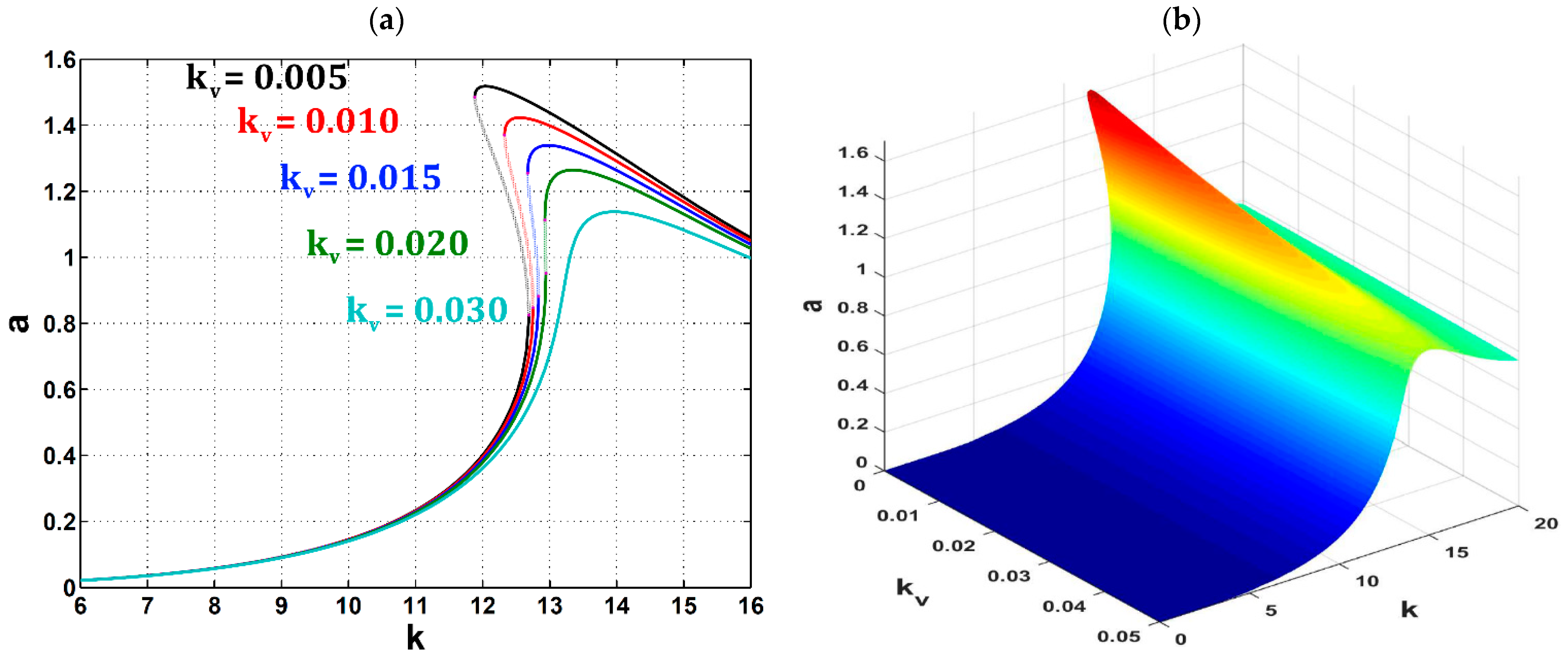
- As the excitation frequency increased, the nonlinear behavior of the force-response curves started to appear with unstable paths that increased gradually from one curve to another one.
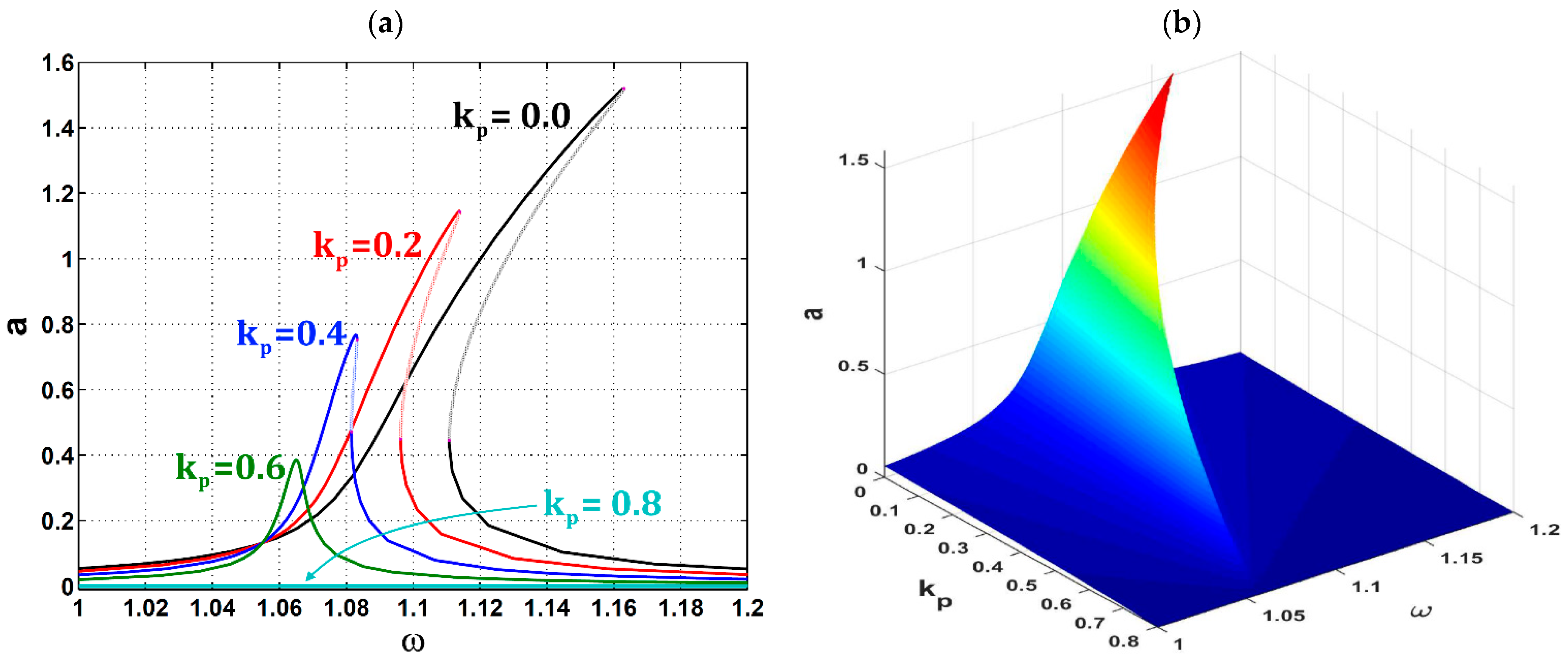
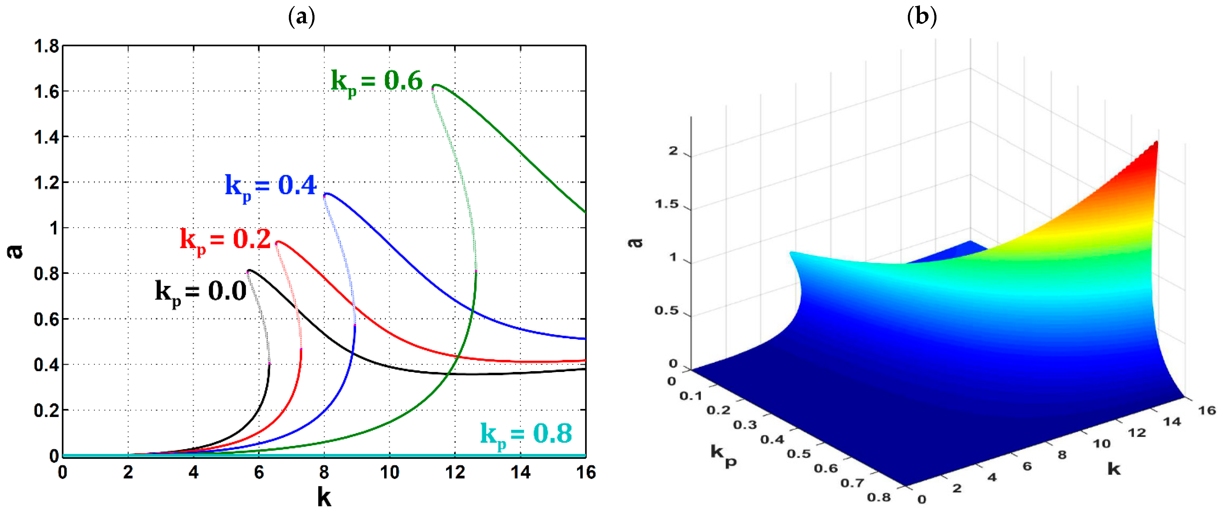
- Raising the CP control gain could cause a reduction in the whole cubic-nonlinearity term leading to suppressing the curve’s peak.
- The trivial car’s amplitude could be reached theoretically in the case that regardless the value of .
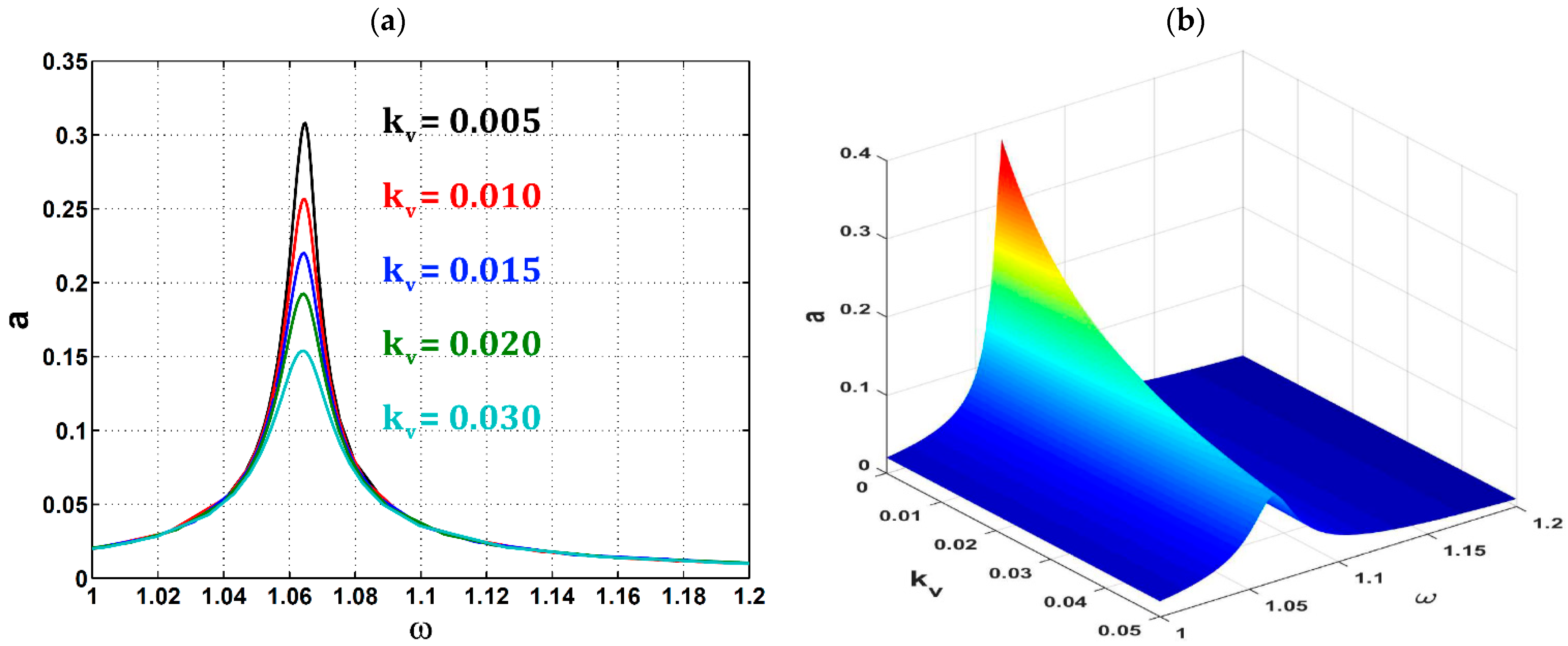
- The NV control gain helped in enhancing the overall damping behavior of the car’s oscillations.
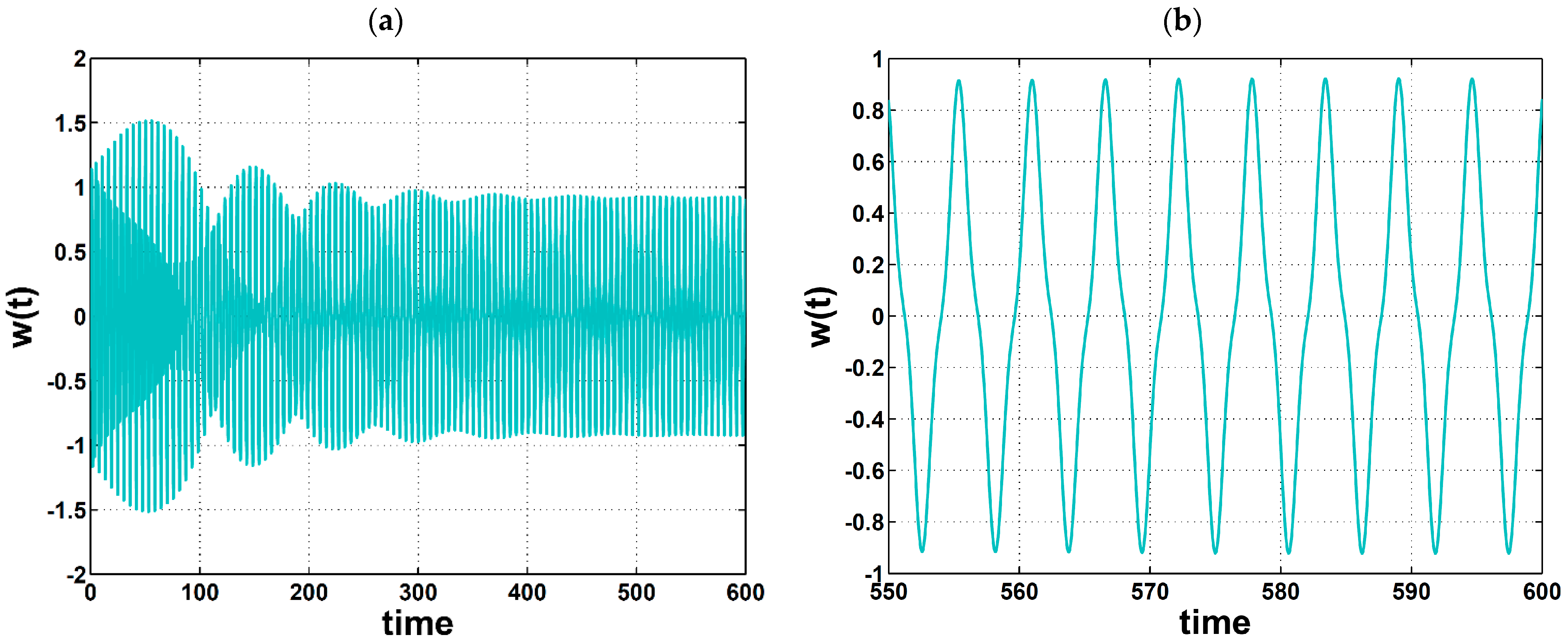
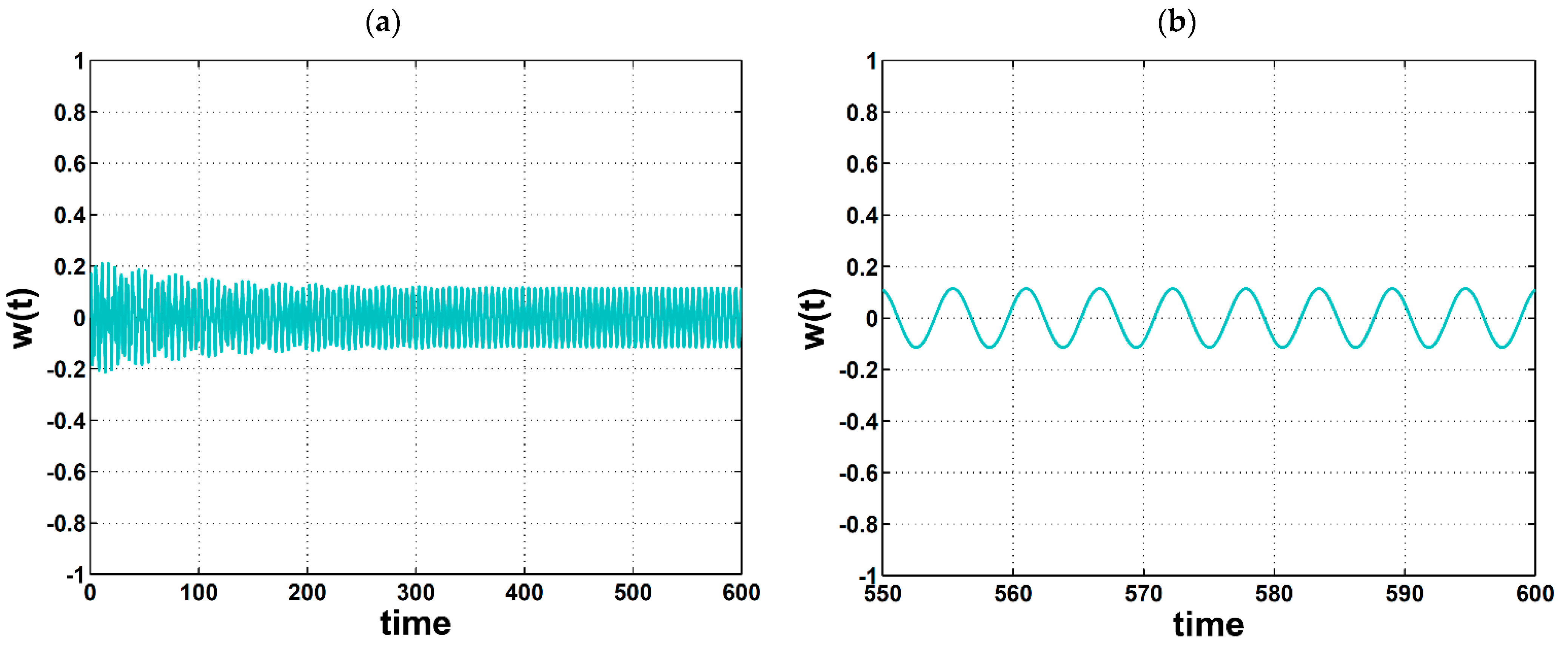
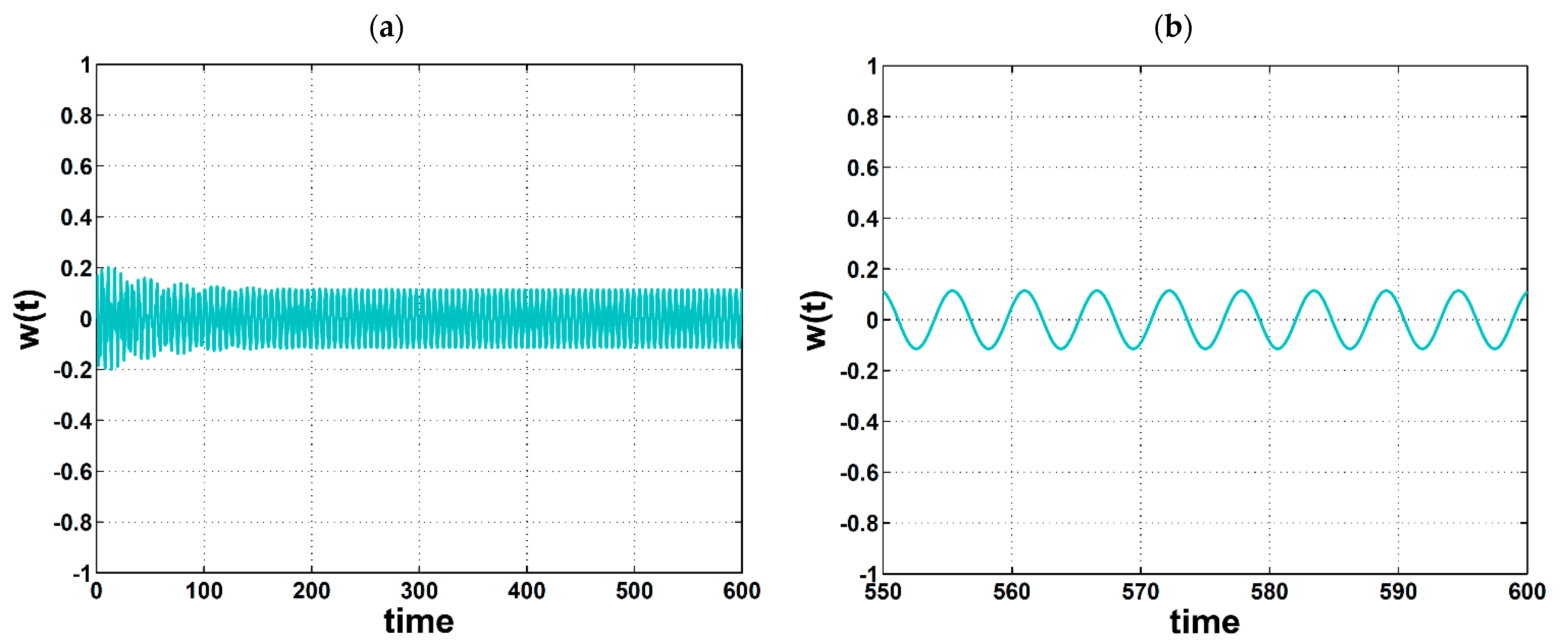
- The car’s steady oscillations were mitigated by about from its former state thanks to the applied controller.
- The car’s transient oscillations ended faster than its former state thanks to the applied controller.
Author Contributions
Funding
Institutional Review Board Statement
Informed Consent Statement
Data Availability Statement
Acknowledgments
Conflicts of Interest
References
- Rahman, Z.; Burton, T.D. Large amplitude primary and superharmonic resonances in the Duffing oscillator. J. Sound Vib. 1986, 110, 363–380. [Google Scholar] [CrossRef]
- Nayfeh, A.H.; Sanchez, N.E. Bifurcations in a forced softening duffing oscillator. Int. J. Non-Linear Mech. 1989, 24, 483–497. [Google Scholar] [CrossRef]
- Benedettini, F.; Rega, G. Planar non-linear oscillations of elastic cables under superharmonic resonance conditions. J. Sound Vib. 1989, 132, 353–366. [Google Scholar] [CrossRef]
- Burton, T.D.; Anderson, M. On asymptotic behavior in cascades chaotically excited non-linear oscillators. J. Sound Vib. 1989, 133, 353–358. [Google Scholar] [CrossRef]
- Rahman, Z.; Burton, T.D. On higher order methods of multiple scales in non-linear oscillations-periodic steady state response. J. Sound Vib. 1989, 133, 369–379. [Google Scholar] [CrossRef]
- Sanchez, N.E.; Nayfeh, A.H. Prediction of bifurcations in a parametrically excited duffing oscillator. Int. J. Non-Linear Mech. 1990, 25, 163–176. [Google Scholar] [CrossRef]
- Rega, G.; Benedettini, F.; Salvatori, A. Periodic and chaotic motions of an unsymmetrical oscillator in nonlinear structural dynamics. Chaos Solitons Fractals 1991, 1, 39–54. [Google Scholar] [CrossRef]
- Gottlieb, O.; Yim, S.C.S. Nonlinear oscillations, bifurcations and chaos in a multi-point mooring system with a geometric nonlinearity. Appl. Ocean Res. 1992, 14, 241–257. [Google Scholar] [CrossRef]
- Hamdan, M.N.; Burton, T.D. On the Steady State Response and Stability of Non-Linear Oscillators Using Harmonic Balance. J. Sound Vib. 1993, 166, 255–266. [Google Scholar] [CrossRef]
- Hassan, A. On the Third Superharmonic Resonance in the Duffing Oscillator. J. Sound Vib. 1994, 172, 513–526. [Google Scholar] [CrossRef]
- Addison, P.S. On the characterization of non-linear oscillator systems in chaotic mode. J. Sound Vib. 1995, 179, 385–398. [Google Scholar] [CrossRef]
- Adrezin, R.; Bar-Avi, P.; Benaroya, H. Dynamic Response of Compliant Offshore Structures—Review. J. Aerosp. Eng. 1996, 9, 114–131. [Google Scholar] [CrossRef]
- Lukomsky, V.P.; Bobkov, V.B. Asymptotic Expansions of the Periodic Solutions of Nonlinear Evolution Equations. Nonlinear Dyn. 1998, 16, 1–21. [Google Scholar] [CrossRef]
- Vaidya, P.G.; He, R. An analysis of the trans-spectral-coherence for duffing oscillators undergoing chaos. J. Sound Vib. 1998, 212, 435–454. [Google Scholar] [CrossRef]
- Luongo, A.; Paolone, A. On the Reconstitution Problem in the Multiple Time-Scale Method. Nonlinear Dyn. 1999, 19, 135–158. [Google Scholar] [CrossRef]
- Al-Qaisia, A.A.; Hamdan, M.N. On the steady state response of oscillators with static and inertia non-linearities. J. Sound Vib. 1999, 223, 49–71. [Google Scholar] [CrossRef]
- Khanin, R.; Cartmell, M.; Gilbert, A. A computerised implementation of the multiple scales perturbation method using Mathematica. Comput. Struct. 2000, 76, 565–575. [Google Scholar] [CrossRef]
- Hamdan, M.N.; Al-Qaisia, A.A.; Al-Bedoor, B.O. Comparison of analytical techniques for nonlinear vibrations of a parametrically excited cantilever. Int. J. Mech. Sci. 2001, 43, 1521–1542. [Google Scholar] [CrossRef]
- Nielsen, S.R.K.; Kirkegaard, P.H. Super and combinatorial harmonic response of flexible elastic cables with small sag. J. Sound Vib. 2002, 251, 79–102. [Google Scholar] [CrossRef] [Green Version]
- Cartmell, M.P.; Ziegler, S.W.; Khanin, R.; Forehand, D.I.M. Multiple scales analyses of the dynamics of weakly nonlinear mechanical systems. Appl. Mech. Rev. 2003, 56, 455–492. [Google Scholar] [CrossRef]
- Rega, G. Nonlinear vibrations of suspended cables—Part I: Modeling and analysis. Appl. Mech. Rev. 2004, 57, 443–478. [Google Scholar] [CrossRef]
- Berlioz, A.; Lamarque, C.-H. A non-linear model for the dynamics of an inclined cable. J. Sound Vib. 2005, 279, 619–639. [Google Scholar] [CrossRef]
- Wang, J.J.; Zhu, S.J.; Liu, S.Y. Study on the mechanism for line spectrum reduction in nonlinear vibration isolation system. In Proceedings of the ASME International Design Engineering Technical Conferences & Computers and Information in Engineering, Las Vegas, NV, USA, 4–7 September 2007; pp. 1349–1354. [Google Scholar]
- Kovacic, I.; Brennan, M.J.; Lineton, B. On the resonance response of an asymmetric Duffing oscillator. Int. J. Non-Linear Mech. 2008, 43, 858–867. [Google Scholar] [CrossRef]
- Macdonald, J.H.G.; Dietz, M.S.; Neild, S.A.; Gonzalez-Buelga, A.; Crewe, A.J.; Wagg, D.J. Generalised modal stability of inclined cables subjected to support excitations. J. Sound Vib. 2010, 329, 4515–4533. [Google Scholar] [CrossRef]
- Dankowicz, H.; Lacarbonara, W. On various representations of higher order approximations of the free oscillatory response of nonlinear dynamical systems. J. Sound Vib. 2011, 330, 3410–3423. [Google Scholar] [CrossRef]
- Vassilopoulou, I.; Gantes, C.J. Nonlinear dynamic phenomena in a SDOF model of cable net. Ingenieur-Archiv 2012, 82, 1689–1703. [Google Scholar] [CrossRef]
- Dai, H.-H.; Yue, X.-K.; Yuan, J.-P. A time domain collocation method for obtaining the third superharmonic solutions to the Duffing oscillator. Nonlinear Dyn. 2013, 73, 593–609. [Google Scholar] [CrossRef]
- Huang, X.; Liu, X.; Sun, J.; Zhang, Z.; Hua, H. Vibration isolation characteristics of a nonlinear isolator using Euler buckled beam as negative stiffness corrector: A theoretical and experimental study. J. Sound Vib. 2014, 333, 1132–1148. [Google Scholar] [CrossRef]
- Ozcelik, O.; Attar, P.J. Nonlinear response of flapping beams to resonant excitations under nonlinear damping. Acta Mech. 2015, 226, 4281–4307. [Google Scholar] [CrossRef]
- Sari, M.S. Superharmonic resonance analysis of nonlocal nano beam subjected to axial thermal and magnetic forces and resting on a nonlinear elastic foundation. Microsyst. Technol. 2017, 23, 3319–3330. [Google Scholar] [CrossRef]
- Elliott, A.J.; Cammarano, A.; Neild, S.A.; Hill, T.L.; Wagg, D. Comparing the direct normal form and multiple scales methods through frequency detuning. Nonlinear Dyn. 2018, 94, 2919–2935. [Google Scholar] [CrossRef] [PubMed] [Green Version]
- Zhao, Y.; Huang, C.; Chen, L. Nonlinear planar secondary resonance analyses of suspended cables with thermal effects. J. Therm. Stress. 2019, 42, 1–20. [Google Scholar] [CrossRef]
- Kandil, A. Internal resonances among the first three modes of a hinged–hinged beam with cubic and quintic nonlinearities. Int. J. Non-Linear Mech. 2020, 127, 103592. [Google Scholar] [CrossRef]
- Arena, A.; Lacarbonara, W. Piezoelectrically induced nonlinear resonances for dynamic morphing of lightweight panels. J. Sound Vib. 2021, 498, 115951. [Google Scholar] [CrossRef]
- Kandil, A.; Hamed, Y.S.; Alsharif, A.M.; Awrejcewicz, J. 2D and 3D Visualizations of the Mass-Damper-Spring Model Dynamics Controlled by a Servo-Controlled Linear Actuator. IEEE Access 2021, 9, 153012–153026. [Google Scholar] [CrossRef]
- Su, X.; Kang, H.; Guo, T. Modelling and energy transfer in the coupled nonlinear response of a 1:1 internally resonant cable system with a tuned mass damper. Mech. Syst. Signal Process. 2021, 162, 108058. [Google Scholar] [CrossRef]
- Long, Y.; Kang, H. Analysis of 1:1 internal resonance of a CFRP cable with an external 1/3 subharmonic resonance. Nonlinear Dyn. 2022, 107, 3425–3441. [Google Scholar] [CrossRef]
- Kloda, L.; Lenci, S.; Warminski, J.; Szmit, Z. Flexural–flexural internal resonances 3:1 in initially straight, extensible Timoshenko beams with an axial spring. J. Sound Vib. 2022, 527, 116809. [Google Scholar] [CrossRef]
- Kandil, A.; Hamed, Y.S.; Abualnaja, K.M.; Awrejcewicz, J.; Bednarek, M. 1/3 Order Subharmonic Resonance Control of a Mass-Damper-Spring Model via Cubic-Position Negative-Velocity Feedback. Symmetry 2022, 14, 685. [Google Scholar] [CrossRef]
- Guo, T.; Rega, G. Nonlinear mode localization in boundary–interior coupled structures by an asymptotic approach. Int. J. Non-Linear Mech. 2022, 141, 103929. [Google Scholar] [CrossRef]
- Dalela, S.; Balaji, P.S.; Jena, D.P. Design of a metastructure for vibration isolation with quasi-zero-stiffness characteristics using bistable curved beam. Nonlinear Dyn. 2022, 1–41. [Google Scholar] [CrossRef]
- Nayfeh, A.; Mook, D. Nonlinear Oscillations; Wiley: New York, NY, USA, 1995. [Google Scholar]


Publisher’s Note: MDPI stays neutral with regard to jurisdictional claims in published maps and institutional affiliations. |
© 2022 by the authors. Licensee MDPI, Basel, Switzerland. This article is an open access article distributed under the terms and conditions of the Creative Commons Attribution (CC BY) license (https://creativecommons.org/licenses/by/4.0/).
Share and Cite
Kandil, A.; Hamed, Y.S.; Mohamed, M.S.; Awrejcewicz, J.; Bednarek, M. Third-Order Superharmonic Resonance Analysis and Control in a Nonlinear Dynamical System. Mathematics 2022, 10, 1282. https://doi.org/10.3390/math10081282
Kandil A, Hamed YS, Mohamed MS, Awrejcewicz J, Bednarek M. Third-Order Superharmonic Resonance Analysis and Control in a Nonlinear Dynamical System. Mathematics. 2022; 10(8):1282. https://doi.org/10.3390/math10081282
Chicago/Turabian StyleKandil, Ali, Yasser S. Hamed, Mohamed S. Mohamed, Jan Awrejcewicz, and Maksymilian Bednarek. 2022. "Third-Order Superharmonic Resonance Analysis and Control in a Nonlinear Dynamical System" Mathematics 10, no. 8: 1282. https://doi.org/10.3390/math10081282