Article

Application of Game Method for Modelling and Temporal Intuitionistic Fuzzy Pairs to the Forest Fire Spread in the Presence of Strong Wind

by
Deyan Mavrov
1,†,
Vassia Atanassova
2,*,†,
Veselina Bureva
1,†,
Olympia Roeva
2,†,
Peter Vassilev
2,†,
Radoslav Tsvetkov
3,†,
Dafina Zoteva
4,†,
Evdokia Sotirova
1,†,
Krassimir Atanassov
2,†,
Alexander Alexandrov
5,† and
Hristo Tsakov
5,†
1
Intelligent Systems Laboratory, “Prof. Dr. Assen Zlatarov” University, 1 “Prof. Yakim Yakimov” Blvd., 8010 Burgas, Bulgaria
2
Department of Bioinformatics and Mathematical Modelling, Institute of Biophysics and Biomedical Engineering, Bulgarian Academy of Sciences, Acad. Georgi Bonchev Str., Bl. 105, 1113 Sofia, Bulgaria
3
Faculty of Applied Mathematics and Informatics, Technical University Sofia, 8 Kliment Ohridski Blvd., 1000 Sofia, Bulgaria
4
Faculty of Mathematics and Informatics, Sofia University “St. Kliment Ohridski”, 5 James Bourchier Blvd., 1164 Sofia, Bulgaria
5
Department of Agricultural and Forestry Sciences, Forest Research Institute, Bulgarian Academy of Sciences, 132 Kliment Ohridski Blvd., 1756 Sofia, Bulgaria
*
Author to whom correspondence should be addressed.
These authors contributed equally to this work.
Mathematics 2022, 10(8), 1280; https://doi.org/10.3390/math10081280
Submission received: 15 March 2022 / Revised: 1 April 2022 / Accepted: 6 April 2022 / Published: 12 April 2022
(This article belongs to the Section Fuzzy Sets, Systems and Decision Making)

Abstract

:
In a series of papers, the initiation and development of forest fires are described in terms of the cellular automata-based Game Method for Modelling (GMM), modelling a particular area as an orthogonal grid of square cells whose values are changing with respect to predefined rules. In the present leg of this research, the simulation of the wildfire that occurred in the Kresna Gorge in Bulgaria in August 2017 is presented, rendering an account of the wind, characterized by its direction and intensity, and evaluating the impact of the fire iteratively in terms of temporal intuitionistic fuzzy sets that maintain the information about the degrees of burnt and unaffected areas. The results from the software product FireGrid, implementing the GMM-model developed by the authors, are also compared to the results from the software application FlamMap. Additionally, the paper presents for the first time the basic properties of the defined operations and operators over temporal intuitionistic fuzzy pairs.

1. Introduction

Wildfires pose serious problems for every national economy as identified and documented for a number of countries (e.g., Portugal [1], Serbia [2], New Zealand [3]) and whole continents (e.g., Europe [4]). This has made them a natural object of research investigation and modelling using various mathematical tools and paradigms of artificial intelligence such as multiagent systems [5], and stochastic dynamical systems [6]. The main environmental elements that affect wildfire behavior are weather, combustible biomass (fuel) and terrain topography.
The distinct portions of a wildfire can be divided into head, flank and rear. The most active and fastest spreading part of the fire is called the “head”, where naturally a fire may have multiple heads. The opposite, the slowest burning part of the fire is represented as the “rear” (“tail”). The sides of the fire perpendicular to the head and rear present the left and right flanks [7].
Despite the existing extensive research on wildfire modelling, it is still worth finding new approaches for the development of better mathematical models in this regard. One such tool is the Game Method for Modelling (GMM) that has been developed over the last decade [8,9]. The GMM is an extension of John Horton Conway’s Game of Life [10,11], aiming to capture complex behavior while remaining computationally light. The classical Conway’s Game of Life has a “universe” formed by an infinite two-dimensional orthogonal grid of square cells, each of which is in one of two possible states, “alive” or “dead”. GMM modifies the classical CGL by adding much more information to the possible states of the cells and more sophisticated rules of the mutual interaction between the cells leading to changing their states as a way to represent certain behaviors.
The GMM has already been approved as an appropriate tool for modelling of wildfire propagations in a series of papers by the authors. Forest fire perimeter expansion was evaluated in [12], taking into additional consideration the effect of wind [13,14] and the differences in the types of burning vegetation [15]. A literature review further shows that cellular automata have been recently employed to the modelling and simulation of wildfires. In [16], Green et al. perform wildfire modelling using evolutionary cellular automata. Further using the idea of applying cellular automata to wildfire modelling, research is conducted regarding the forests in Amazonia [17], Australia [18], Greece [19] and others.
In a recent investigation of Li et al., another approach involving cellular automata and LSTM neural networks was employed for the key problem of fire management [20].
In the last years, the authors have developed different software implementations of GMM and applied them to different aspects of wildfire development, e.g., in [21,22]. The motivation to use GMM is that, as it has been proved in [9], GMM can represent the functioning and the results of the work of any cellular automaton. In the present paper, the software is extended with the feature to render an account of the presence of strong wind, which was the actual natural condition of the modelled wildfire in the region of Kresna Gorge. Moreover, for the evaluation of the proportion of burned versus unaffected areas, components of intuitionistic fuzzy logic are used [23,24].
For the first time in such an analysis, the authors propose the introduction of temporal, rather than ordinary, intuitionistic fuzzy pairs [24] in order to evaluate the impact of the wildfire and investigate the basic properties of TIFPs. The obtained GMM results are compared to the results from another existing software product, FlamMap [25].
The paper is structured as follows. In Section 2, a short description of the considered wildfire in Bulgaria is given and the results using FlamMap with the data from the discussed wildfire are shown. The concepts of intuitionistic fuzziness, intuitionistic fuzzy pairs and temporal intuitionistic fuzzy pairs are briefly presented in Section 3 and the basic properties of the operations and the modal operators over TIFPs are studied and proven. In Section 4, the GMM method and its application to wildfire propagation under wind conditions are discussed in detail. Section 5 provides details about the model and the simulation and the obtained results are presented in Section 6. Concluding remarks and directions of future research are offered in Section 7.

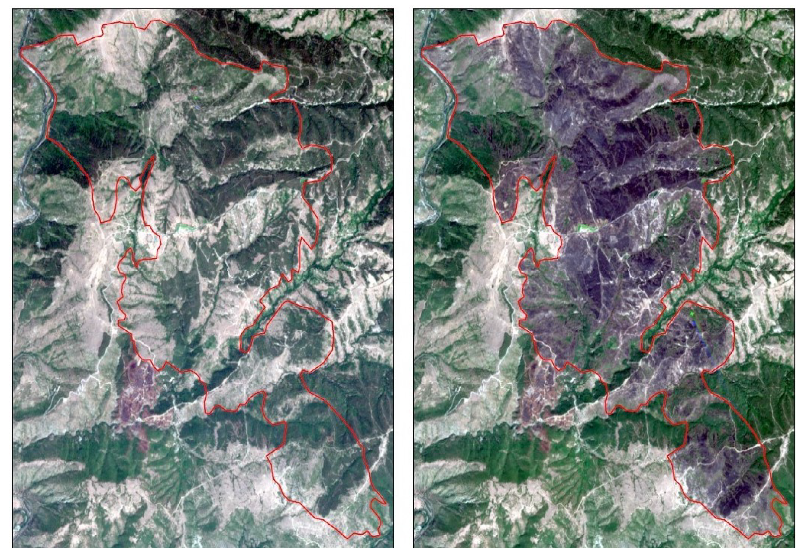
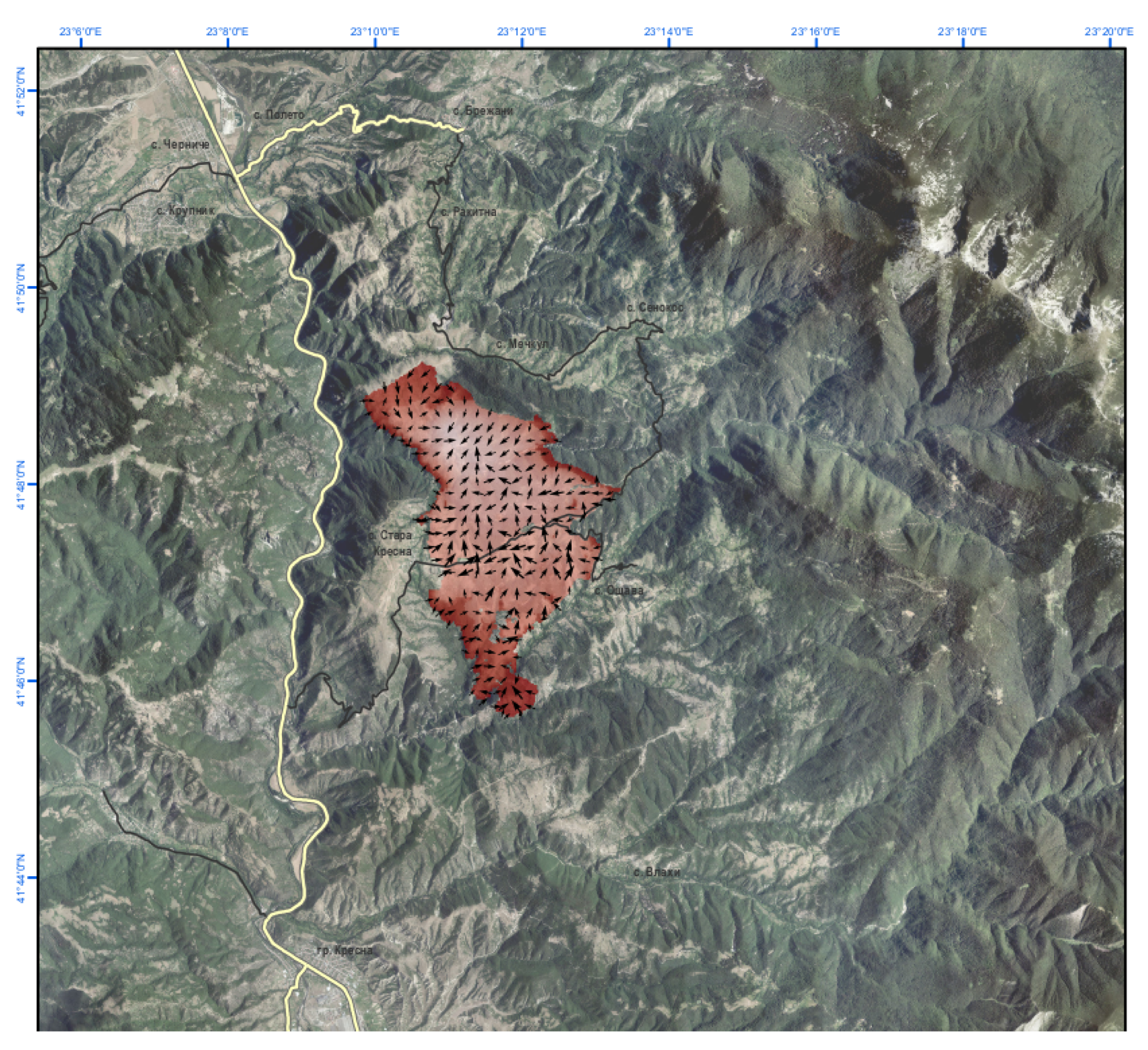
2. Wildfire in the Kresna Gorge, Bulgaria

The wildfire raged in Kresna Gorge on 24–29 August 2017. At this time, during the summer of 2017, the weather in Bulgaria was very dry and hot. The territory of the fire was located east of the Struma River, mainly on the foot of the slope of Pirin Mountain. The fire spread in a southeast direction and at a certain moment of time the flames were high enough to cross the river that flows through the area. The satellite maps of the area before and after the fire are visualized in Figure 1 [26].
In order to run the simulation in FlamMap, a preliminary processing by WindNinja involving the use of a set of raw stationary meteorological data for wind direction and speed, temperature, cloudiness and their weather parameters compared to spatial terrain data using a digital model were performed. The initial data from WindNinja describe the spatial and temporal changes in wind velocity for the considered period in the area of Kresna Gorge. The necessary input data in FlamMap for the characteristics of the Earth’s surface were derived from the digital model data on the specifics of the terrain (digital elemental model, slope, aspect), the density of the canopy cover, a set of models describing flammable materials for different types of land cover, average height of individual forest areas, canopy base height and canopy stand height of different tree species and the density of the dried and green combustible materials in forest vegetation. Additional data needed to develop the model concern the humidity of the dried and green combustible materials, the ignition point and fire lines, which describe the spatial barriers for the fire front that existed in the field during the first 24 h after the fire.
The FlamMap output data are a set of maps tracking the spread of the fire and its intensity. The result of the simulation of the the surface forest fire spread using FlamMap is presented in Figure 2 [25].

3. Definition and Properties of Temporal Intuitionistic Fuzzy Pairs

In the present work, we will apply Temporal Intuitionistic Fuzzy Pairs (TIFP) to the results of the simulation of the GMM model. For the reader’s convenience, we will briefly present the concept of the TIFP.
Let T = { t 1 , t 2 , } be a fixed time-scale with a finite (in the present research) or infinite number of elements. Let E be a fixed universe. The standard Intuitionistic Fuzzy Set (IFS, see [23]) is defined as the object with the form
A = { x , μ A ( x ) , ν A ( x ) | x E } ,
where μ A ( x ) and ν A ( x ) are the degrees of membership (validity, etc.) and of non-membership (non-validity, etc.) of element x E to its subset A, and μ A ( x ) , ν A ( x ) , μ A ( x ) + ν A ( x ) [ 0 , 1 ] . The meaning and importance of these conditions will later be seen when the results from the GMM simulation are visualized in Figures 14–16. For convenience, we also employ the term Intuitionistic Fuzzy Pair (IFP), ref. [24], which is the object x = μ , ν , where μ , ν [ 0 , 1 ] and μ + ν 1 .
In [23], the object
A ( T ) = { x , t , μ A ( x , t ) , ν A ( x , t ) | x E t T }
is defined as a Temporal Intuitionistic Fuzzy Set (TIFS).
By analogy with the IFPs, here, we define the concept of a TIFP by: x ( t ) = a ( t ) , b ( t ) , where a , b : T [ 0 , 1 ] and a ( t ) + b ( t ) 1 for each t T (the above defined time-scale). Its geometrical interpretation is given in Figure 3. For the first time, TIFPs have been mentioned in the context of the GMM modelling of forest fires in [21], but their mathematical properties have not been investigated there. For this purpose, in the present step of the research, we study the TIFPs’ properties and formulate them in three theorems.
Let us have two TIFPs x = a , b and y = c , d , where a , b , c , d : T [ 0 , 1 ] and a ( t ) + b ( t ) 1 , c ( t ) + d ( t ) 1 for each t T . Then, we define analogues of the operations “negation”, “conjunction” and “disjunction”, noting that the “conjunction” and “disjunction” can be defined in different ways, which is a particularity of the intuitionistic fuzzy, compared to ordinary fuzzy, sets:
¬ x ( t ) = b ( t ) , a ( t ) x ( t ) 1 y ( t ) = min ( a ( t ) , c ( t ) ) , max ( b ( t ) , d ( t ) ) x ( t ) 1 y ( t ) = max ( a ( t ) , c ( t ) ) , min ( b ( t ) , d ( t ) ) x ( t ) 2 y ( t ) = a ( t ) + c ( t ) a ( t ) . c ( t ) , b ( t ) . d ( t ) x ( t ) 2 y ( t ) = a ( t ) . c ( t ) , b ( t ) + d ( t ) b ( t ) . d ( t ) .
We additionally need to define here the standard modal operators “necessity” and “possibility” for the case of TIFPs:
x ( t ) = a ( t ) , 1 a ( t ) , x ( t ) = 1 b ( t ) , b ( t ) .
On the basis of these definitions we present here for the first time the basic properties of the operations “negation”, “conjunction” and “disjunction” and operators “necessity” and “possibility” over temporal intuitionistic fuzzy pairs.
Theorem 1.
Let x and y be two TIFPs. Then for each t T :
x ( t ) 1 y ( t ) = ¬ ( ¬ x ( t ) 1 ¬ y ( t ) ) , x ( t ) 1 y ( t ) = ¬ ( ¬ x ( t ) 1 ¬ y ( t ) ) , x ( t ) 2 y ( t ) = ¬ ( ¬ x ( t ) 2 ¬ y ( t ) ) , x ( t ) 2 y ( t ) = ¬ ( ¬ x ( t ) 2 ¬ y ( t ) ) .
Proof. 
Let x and y be given TIFPs and let t T . Then,
¬ ( ¬ x ( t ) 1 ¬ y ( t ) ) = ¬ ( ¬ a ( t ) , b ( t ) ) 1 ¬ c ( t ) , d ( t ) ) ) = ¬ ( b ( t ) , a ( t ) ) 1 d ( t ) , c ( t ) ) ) = ¬ max ( b ( t ) , d ( t ) ) , min ( a ( t ) , c ( t ) ) = min ( a ( t ) , c ( t ) ) , max ( b ( t ) , d ( t ) ) = x ( t ) 1 y ( t ) .
The rest of the statements as well as the following two theorems are proven in the same manner. □
Theorem 2.
Let x be a TIFP. Then, for each t T :
x ( t ) = ¬ ( ¬ x ( t ) ) , x ( t ) = ¬ ( ¬ x ( t ) ) .
Theorem 3.
Let x and y be two TIFPs. Then for each t T :
( x ( t ) 1 y ( t ) = ( x ( t ) 1 y ( t ) , ( x ( t ) 1 y ( t ) = ( x ( t ) 1 y ( t ) , ( x ( t ) 2 y ( t ) = ( x ( t ) 2 y ( t ) , ( x ( t ) 2 y ( t ) = ( x ( t ) 2 y ( t ) , ( x ( t ) 1 y ( t ) = ( x ( t ) 1 y ( t ) , ( x ( t ) 1 y ( t ) = ( x ( t ) 1 y ( t ) , ( x ( t ) 2 y ( t ) = ( x ( t ) 2 y ( t ) , ( x ( t ) 2 y ( t ) = ( x ( t ) 2 y ( t ) .
For a fixed IFP x, we can define the set of TIFPs by:
{ x ( t ) , μ ( t ) , ν ( t ) | t T }
and, obviously, this set is an ordinary IFS with universe T, illustrated in Figure 4. Notably, TIFPs have analogues of all the properties exhibited by the standard IFPs, as described in [24].
Below, in Section 5, we illustrate the way of using TIFPs with an example related to the application of GMM to the data from a real-life wildfire scenario. Particularly, we will use TIFPs to represent each of the iterations of the wildfire spread, and all of these TIFPs will show how they form a particular TIFS, which will be discussed in Section 6.

4. Game Method for Modelling

4.1. GMM Basics

Standardly, GMM uses an infinite two-dimensional orthogonal grid of cells [8]. Depending on the modeled surface, the cells are initially assigned different values. The algorithm for applying the GMM is described in detail in [8].
In the present case, the grid of cells represents the forest fire map. The GMM uses a set of objects, represented by symbols that are placed on the vertices on the grid as well as a set of rules A. Each object is represented by a number, an n-tuple of coordinates representing its location in the grid. In the current application, the cells of water are denoted as R for River and L for Lake. The cells representing rocky areas (stones) are denoted by the letter S. These symbols will remain unchanged during the whole simulation. The numbers from 1 to 9 are written in the cells, representing the homogeneity of the grassy and forested area, where the number 1 indicates the presence of thin vegetation like grasses, isolated shrubs or trees, and the number 9 marks the occurrence of very dense vegetation, i.e., highly combustible forest mass. The cells in the grid interact with their adjacent neighbors in the vertical and horizontal—and sometimes diagonal—directions. When a cell is affected by the fire, at each iteration its numerical value decrements by 1, or reaches the number 0 (for a completely devastated area).
The rules for changing the symbols during the fire have the following form:
[A.1.]
R R ;
[A.2.]
L L ;
[A.3.]
S S ;
[A.4.]
n n 1 , for n [ 1 , 9 ] .

4.2. Application of GMM to Forest Fire Spread in the Presence of Wind

On the first step of the algorithm, the fire occurs in a single cell of the grid, which is represented by its value being decremented with 1.
On each subsequent step of the algorithm, we: (1) define the borders of the zone that will be affected by fire spread, and (2) reassign the values of the the cells within that zone.
(1)
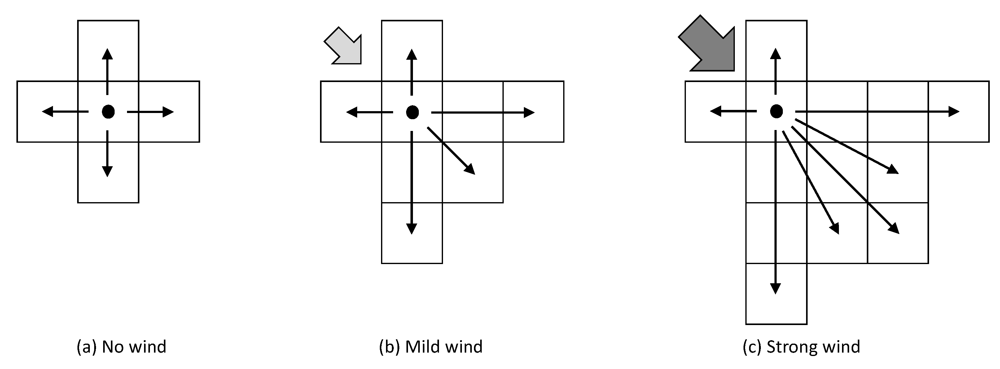
The way of defining the new borders of the fire spread zone is visualized in Figure 5 for the three idealized cases of: (a) no fire, (b) mild wind, or (c) strong wind. (Nota bene: Here we visualize the three cases specifically for northwest wind).
In particular, for every currently affected cell at this step, its own zone of subsequent fire spread is expanded:
(a)
with its four neighbouring cells, as shown in Figure 5a;
(b)
with its four neighbouring cells and the additional three cells in the direction of the mild wind as shown in Figure 5b, i.e., each currently burning cell affects seven other cells at the subsequent iteration;
(c)
with its four neighbouring cells and the additional eight cells in the direction of the strong wind as shown in Figure 5c, i.e., each currently burning cell affects 12 other cells at the subsequent iteration.
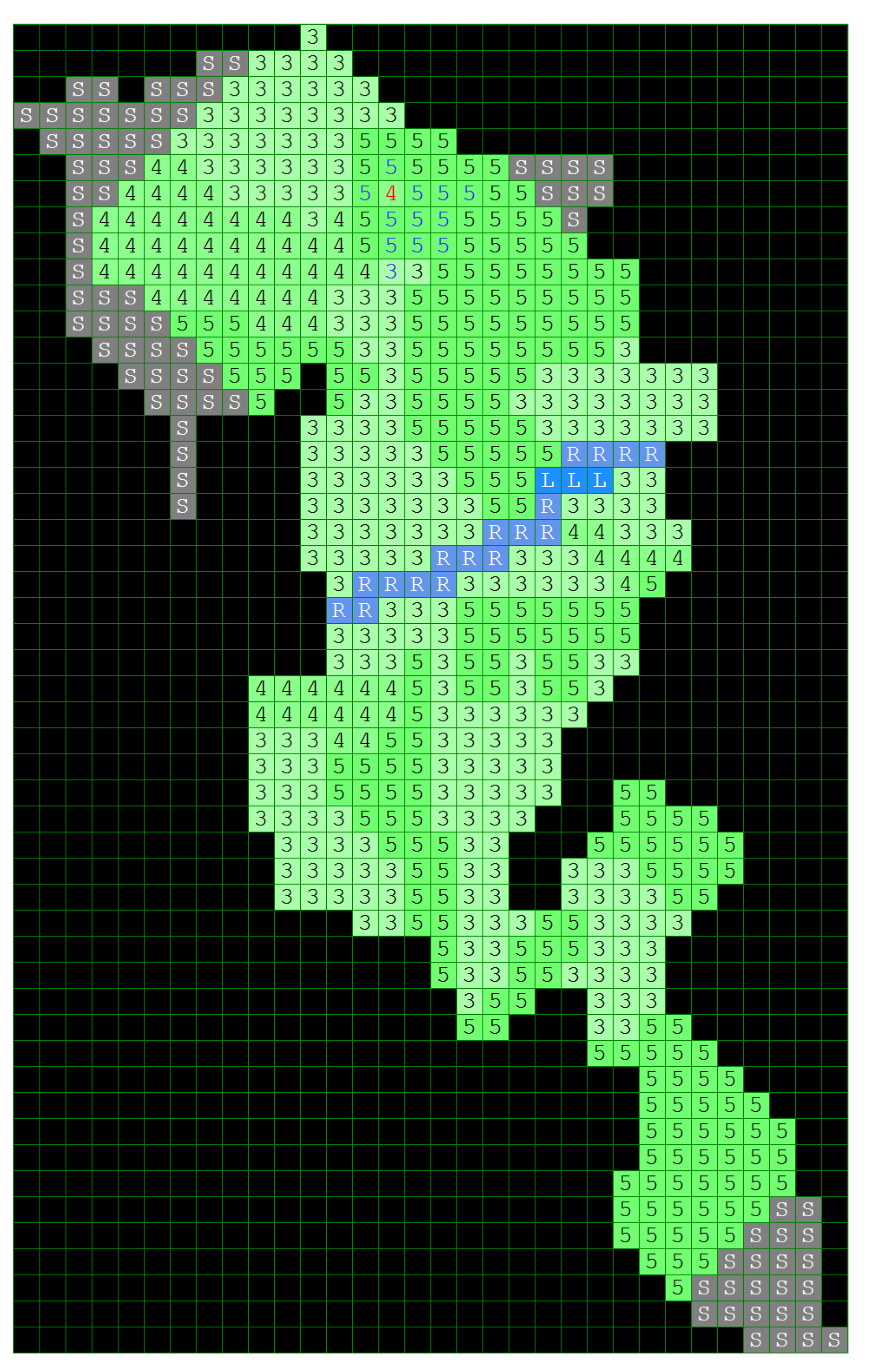
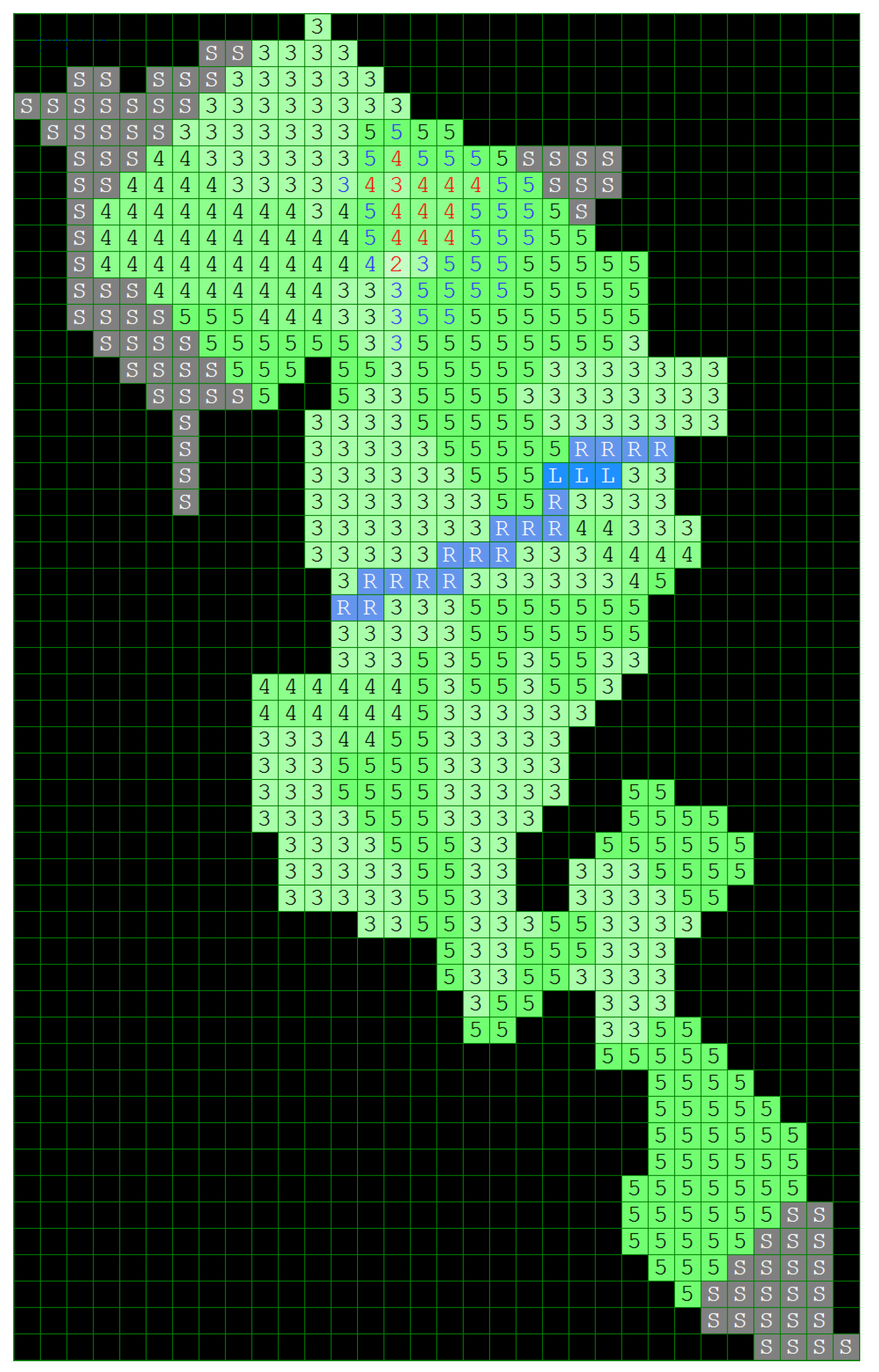
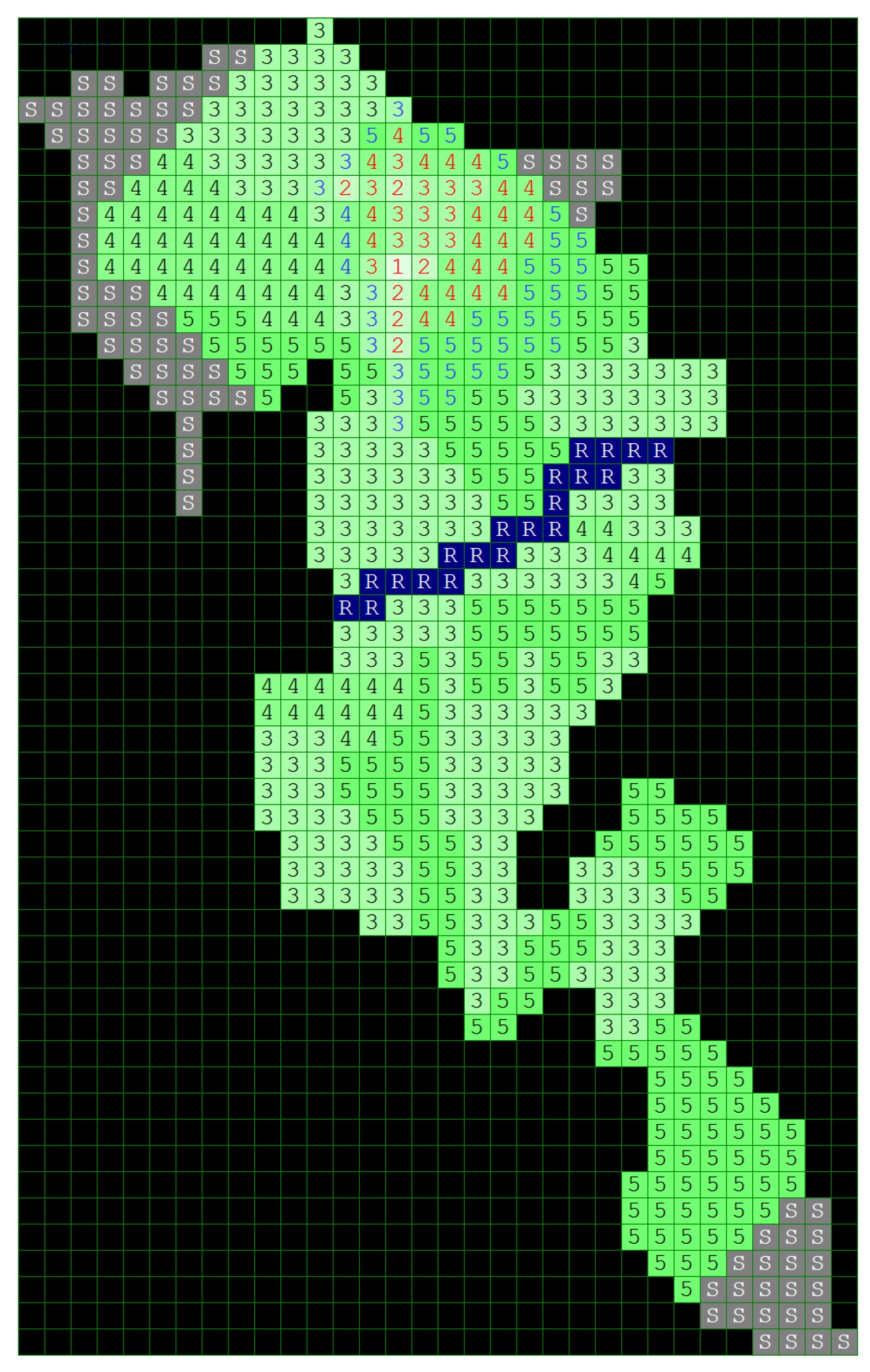
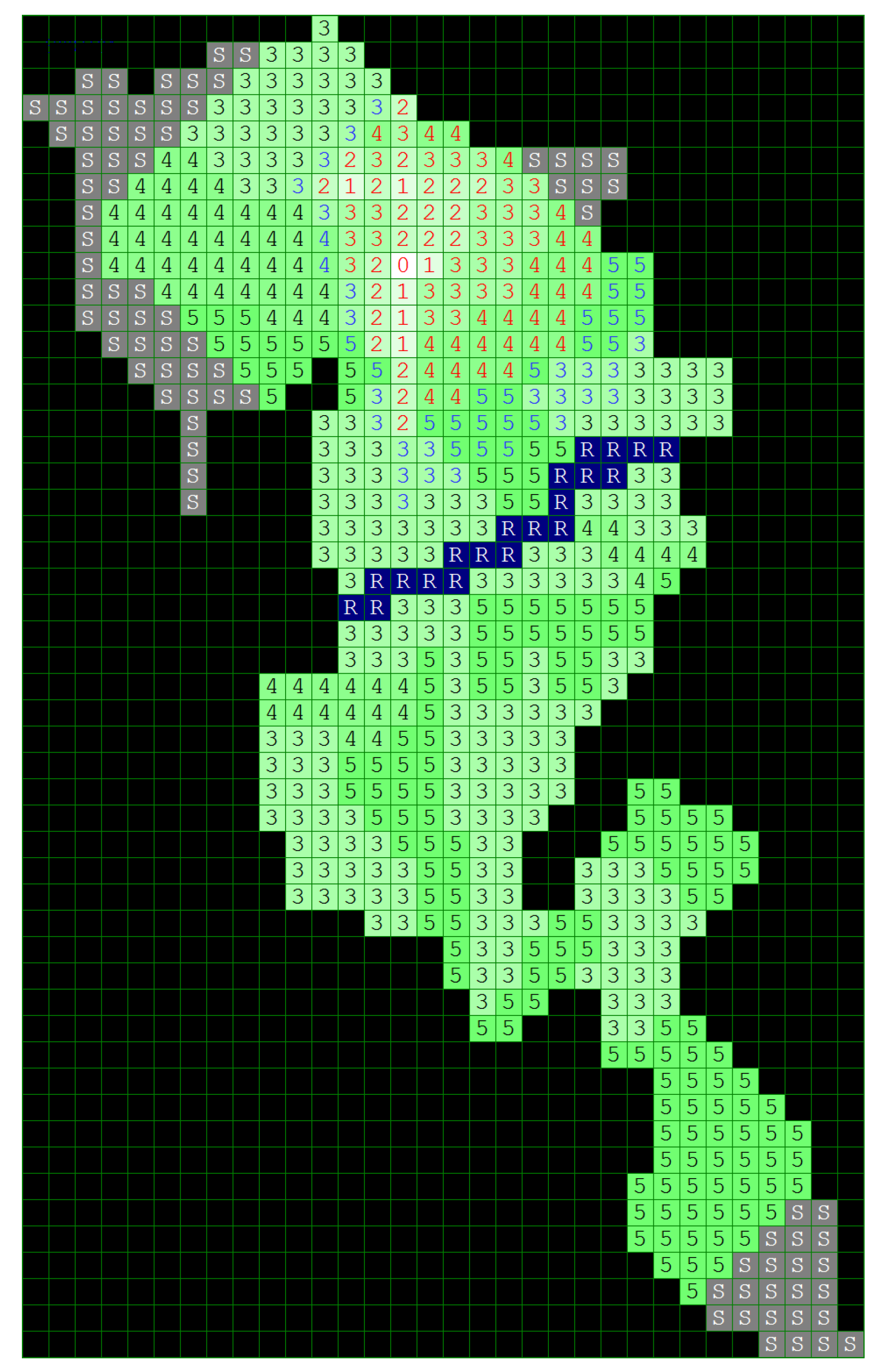
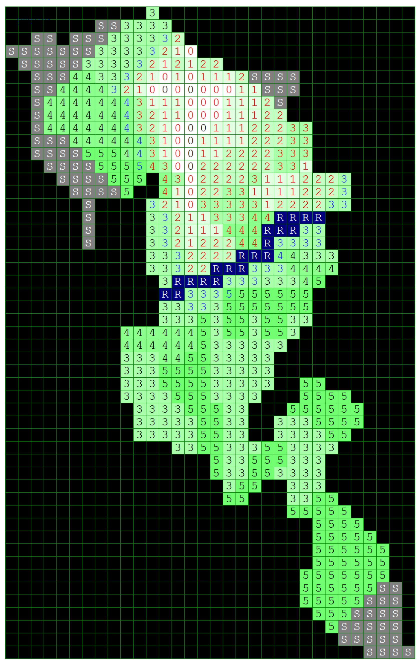
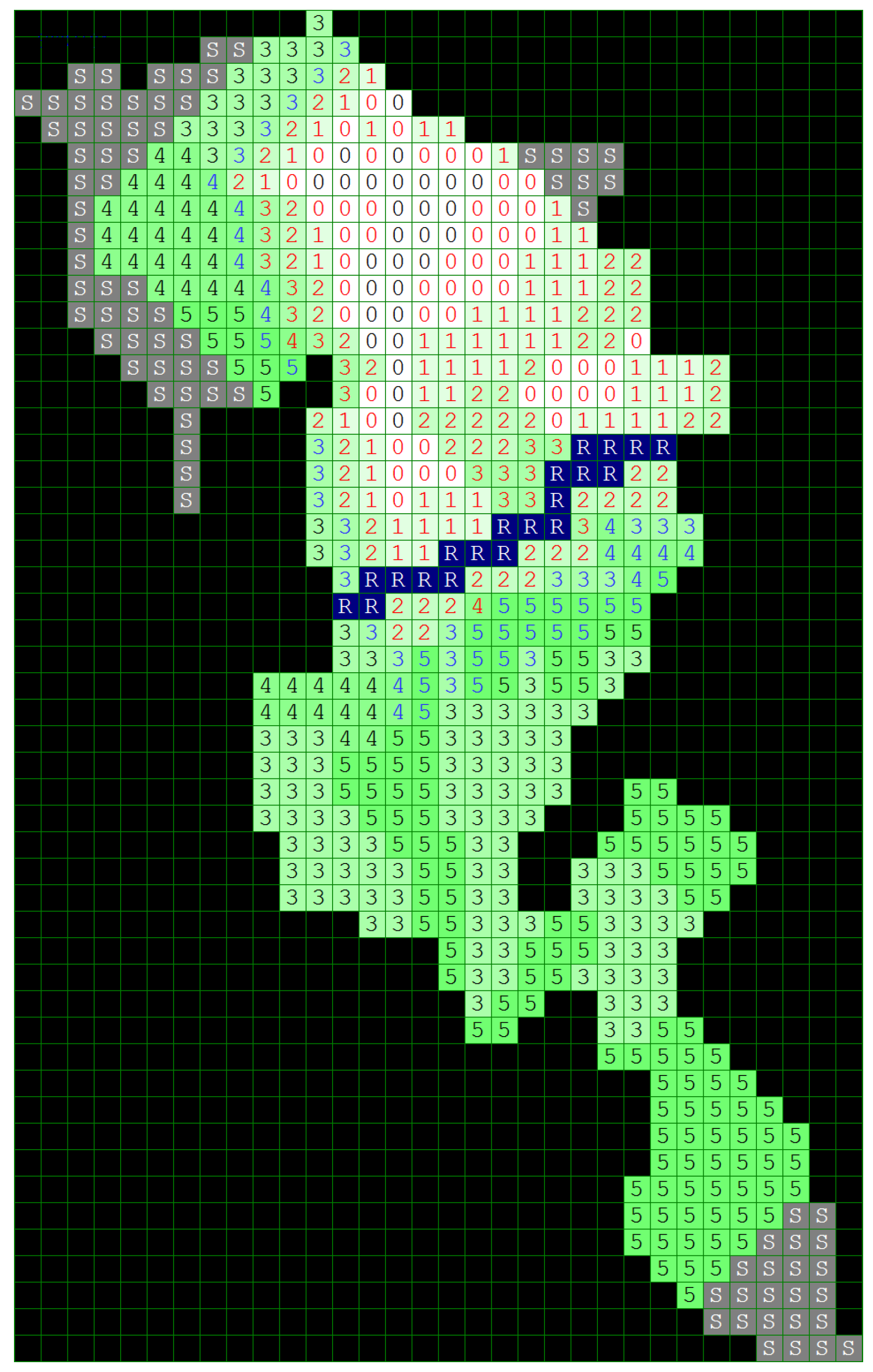
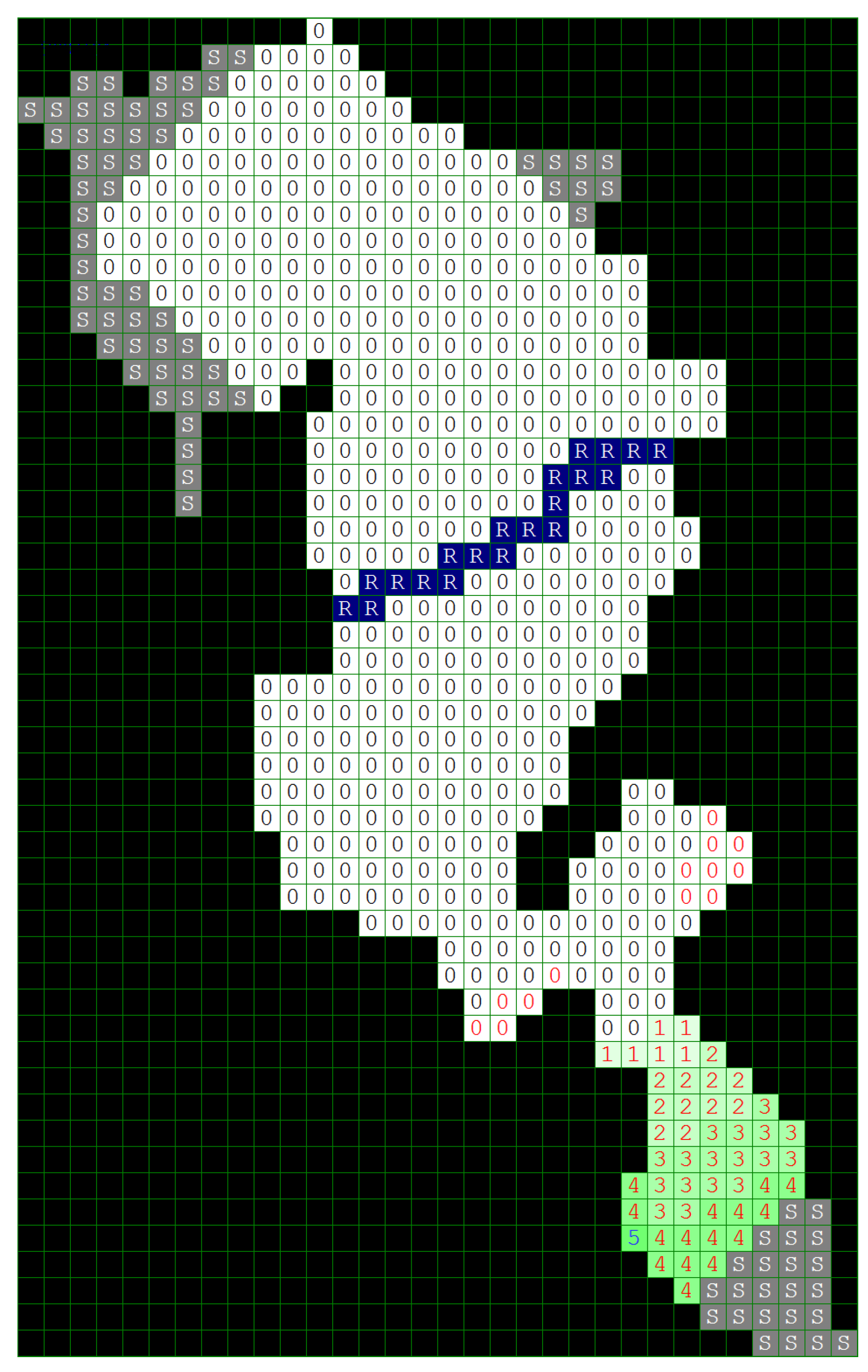
When these zones of subsequent fire spread are defined for all the currently affected (burning) cells at this step, the cumulative area, obtained as a union of these zones, defines the complete zone that at the next step will be affected (burning).
(2)
Burning is represented by:
either leaving them as unchanged (according to rules [A.1.] to [A.3.] from Section 4.1) for unaffectable cells such as R , L or S,
or decrementing them by 1 (according to rule [A.4.]) for the cells that are affectable, i.e., represent combustible forest mass labeled with a number in the [ 1 , 9 ] interval with respect to the density of the “fuel”;
(3)
The algorithm terminates when all the cells in the grid reach the value of 0, meaning that all cells containing any flammable material have already burnt out, and/or the remaining cells are ones that may not be affected by the firespread.

5. Model and Simulation

In this paper, the Game Method of Modelling is applied using the available data regarding the propagation of a particular wildfire, that is, the Kresna Gorge on 24–29 August 2017. The investigated area containing the wildfire represents a grid of 540 cells of potentially flammable forest mass, partly surrounded by a rocky terrain. The cells corresponding to the forest mass are assigned here values from 3 to 5 (representing sparse to mid-dense vegetation), and are colored in green. The rocky areas (stones) are marked with the letter S and the gray color of the cells. The river and the lake in the middle of the region where the fire occurred and developed are denoted in the grid by cells colored blue and marked with the letters R and L, respectively.
In terms of topography, the mountain terrain reflects the fire spread as flames burn uphill faster than they burn downhill, as the heat radiating from the wildfire pre-heats and dries the fuel mass on the slope ahead of the fire, causing it to start burning more rapidly. In the present model, however, due to the relatively sparse vegetation, this terrain’s specifics have been essentially ignored, paying attention to the presence of wind as a more substantial factor for the fire spread. Wind in the real-life situation was characterised as strong and at the location of the ignition point it was with the northwest–southeast direction, which in terms of the GMM apparatus is modelled as illustrated in the schemes of Figure 5c (see (a) for the case of no wind and (b) for the case of mild wind).
In terms of time, the actual wildfire took approximately five full days to spread before it ceased, which—given the total number of 21 intermediate iterations of the model simulation—makes approximately 6 h per iteration.
For the i-th iteration we determined the TIFP μ ( i ) , ν ( i ) that represents an ordered pair composed of the degree of the totally burned area (the number of the totally burned cells divided by the number of all cells) and the degree of the yet unaffected area (the number of the unaffected cells divided by the number of all cells) for the whole considered area at that time-moment. Therefore, the remaining intuitionistic fuzzy degree of hesitation (uncertainty), which is equal to the complement of these two degrees to 1, i.e., π ( i ) = 1 μ ( i ) ν ( i ) , corresponds to the number of currently burning cells of the area divided by the number of all cells. Obviously, before the outburst of the fire, the as yet unaffected area is represented as the TIFP μ ( 0 ) , ν ( 0 ) = 0 , 1 , meaning that none of the land has burned and the whole of it is still intact. At the final iteration, when the whole area has been devastated, the respective TIFP’s value is 1 , 0 .

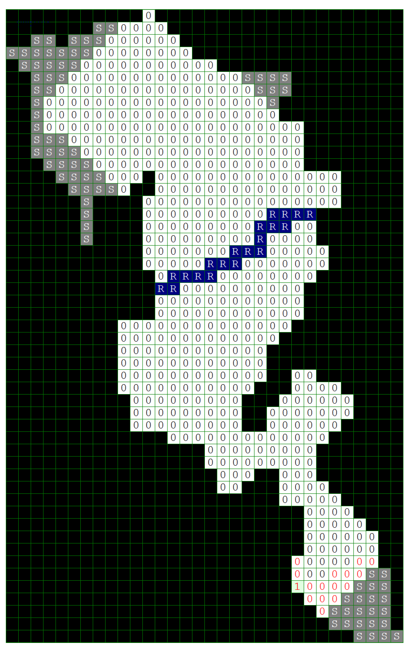
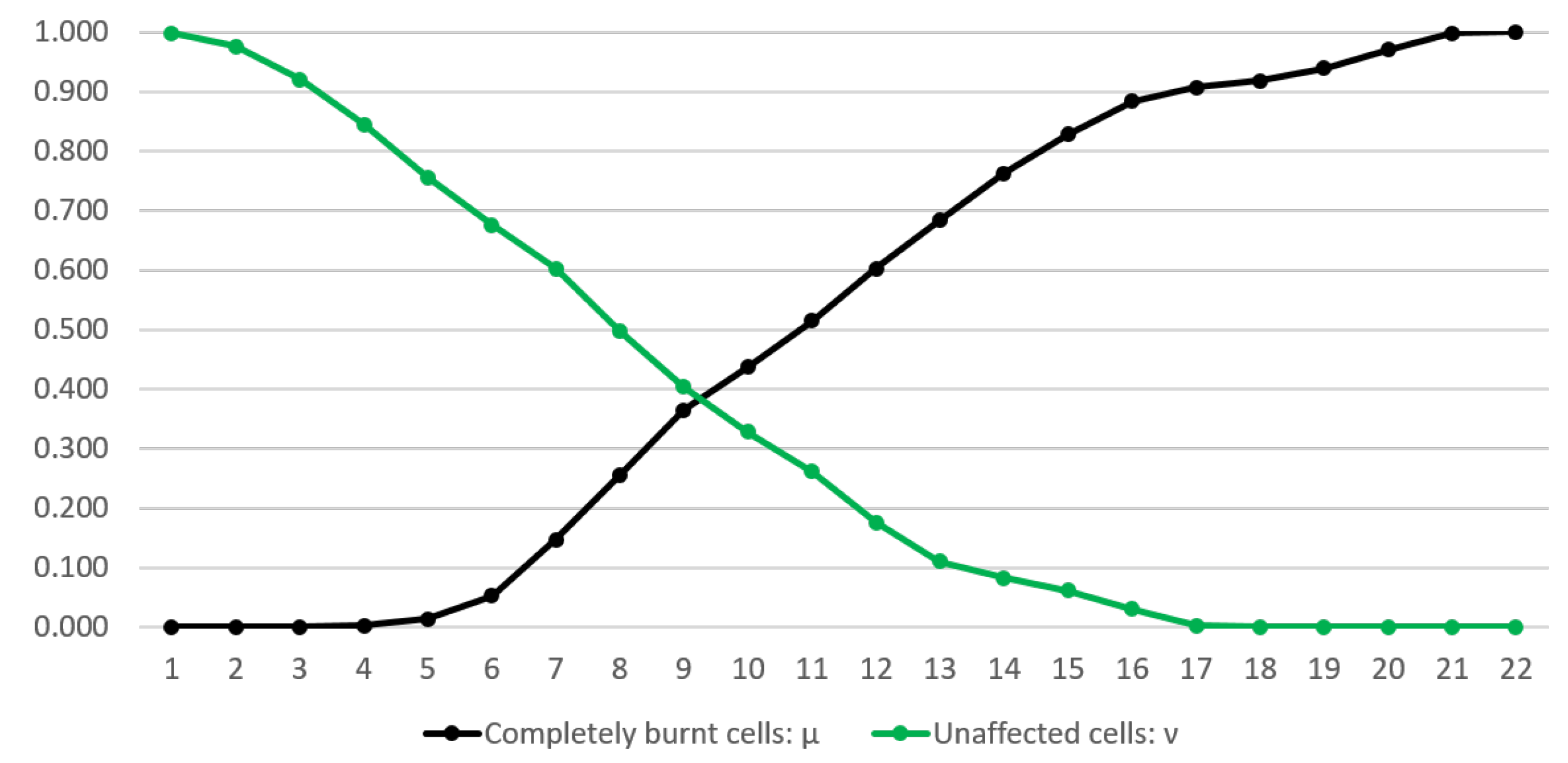
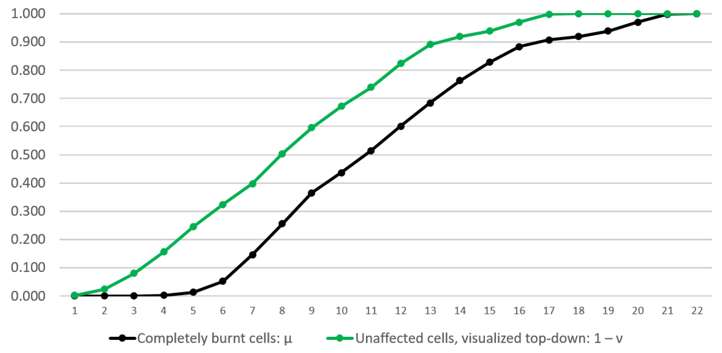
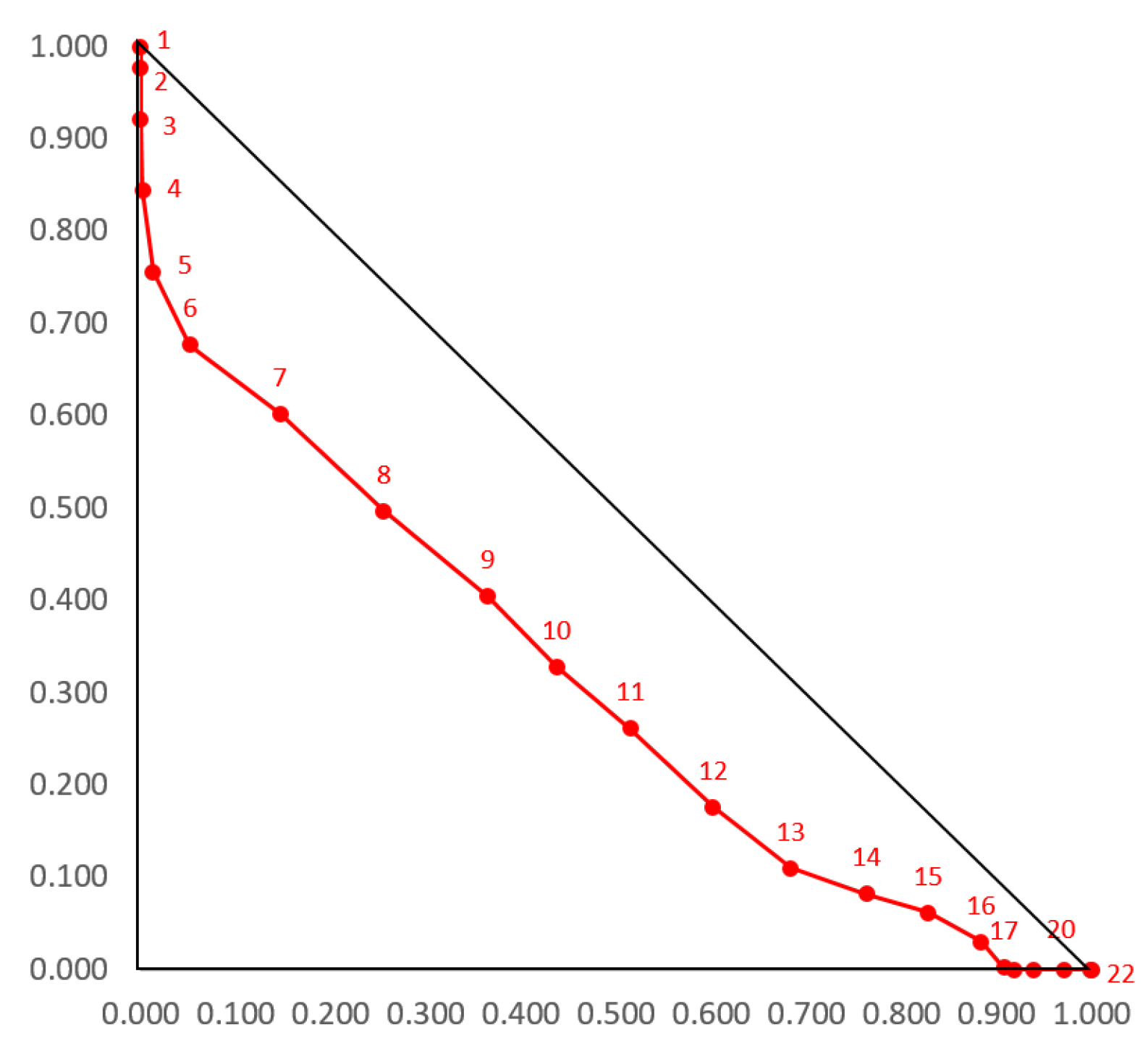
6. Results and Discussion

In what follows, we will present certain iterations from the wildfire spread simulation by GMM, with their respective temporal intuitionistic fuzzy pairs, which are of interest for the fire development and can be generally informative regarding the model’s behavior. The full course of wildfire development in a total number of 22 iterations is presented as a dataset available online at https://forestfires.info/simulations/nw-strong (accessed on 14 March 2022). All the visualizations in that video and the imagery from Figure 6, Figure 7, Figure 8, Figure 9, Figure 10, Figure 11, Figure 12 and Figure 13 in the paper are generated using the F i r e G r i d software for a 2D fire spread simulation using the GMM [27].
The first iteration (see Figure 6) of the modelled development of the wildfire consists of assigning the ignition point. The cell of the ignition point is highlighted in red and its exact location is calculated on the basis of the satellite map (Figure 1). By the rules of GMM, its initially assigned value 5 is decremented by 1 and is now 4. Since at this iteration only one cell is affected, the TIFP has the value μ ( 1 ) , ν ( 1 ) = 0 , 539 540 = 0 , 0.998
The second iteration is visualized in Figure 7, and this is the moment when the model furthermore starts rendering an account of the impact of wind, in accordance with the algorithm presented in Section 4.2 and the wind scheme presented in Figure 5c. The burning cells are 13 and the unaffected ones are 527, with no completely burnt cells, producing the respective TIFP of this iteration, μ ( 2 ) , ν ( 2 ) = 0 , 527 540 = 0 , 0.976
While we will not present every iteration of the wildfire development separately, we will here specifically comment on several moments that are of particular interest.
Particularly interesting moments of the wildfire’s development—from the viewpoint of the modelled process—are the moments when the fire reaches the surrounding rocky areas (Iteration 3), marked with S, and the river and lake, marked with R and L, respectively (Iteration 6). Such areas are naturally occurring “firebreaks”, as there is a lack of vegetation or “fuel” in there. We will furthermore discuss why and how the fire crosses the river/lake and continues southwards (Iteration 7).
Another particularly interesting moment—this time from the point of view of the behavior of the TIFPs—is the first moment when a completely burnt cell occurs (Iteration 5), and the moment when there are no more unaffected cells in the grid (Iteration 18), i.e., all cells are either currently burning or have completely burnt out. Finally, we will show the penultimate Iteration 21, right before the fire stops.
At Iteration 3, we have the first moment when the wildfire reaches a rocky area, see Figure 8. At this step, we have cells that are burning but not yet ones that have completely burnt out. This is why the TIFP that corresponds to this iteration is μ ( 3 ) , ν ( 3 ) = 0 , 497 540 = 0 , 0.920 .
At Iteration 4 (Figure 9), we have the first 1 completely burnt cell, when the number of unaffected cells is 456 and the number of currently burning cells (corresponding in IFS terms to uncertainty π ) is 83, thus producing the TIFP μ ( 4 ) , ν ( 4 ) = 1 540 , 456 540 = 0.002 , 0.844 .
The next particularly notable moments of the wildfire development are Iterations 6 and 7, where the wildfire reaches the banks of the lake and the river (Iteration 6), and crosses them to continue spreading in a southeast direction (Iteration 7). This is noteworthy, since both the river and the lake are relatively small compared to the area affected by the wildfire and the fire intensity by the moment the shores were reached; they have been easily overcome (as potential “firebreaks”) by the actual modelled wildfire, which is the reason why in our model this aspect is simplified and the fire propagates across the cells with no additional modification of the rules.
Later, in Iteration 6 (Figure 10), we have 28 completely burnt cells and 365 unaffected cells with TIFP μ ( 6 ) , ν ( 6 ) = 28 540 , 365 540 = 0.052 , 0.676 .
In the following Iteration 7 (Figure 11), we have 79 completely burnt cells and 325 unaffected cells with TIFP μ ( 7 ) , ν ( 7 ) = 79 540 , 325 540 = 0.146 , 0.602 .
Nevertheless, we shall note that modelling the wildfire spread across natural barriers (such as river streams, lakes, stone runs or canyons) or anthropogenic barriers (such as road infrastructure or artificial firebreaks as a result of logging) deserves separate attention and will be a matter of investigation at a later stage of our research. It is noteworthy that in certain cases fire may spread across seemingly impenetrable divides—there are notable cases in history such as the 1988 fires in Yellowstone National Park, when hot embers managed to cross the Lewis Canyon, a natural canyon more than a kilometer wide and 180 meters deep [28]. Hence, careful consideration is necessary both regarding the width and depth of the barrier, the terrain and the type of the fire [29] but also humidity (fuel moisture) as an additional factor when modelling some of the barriers of wildfire propagation like river streams [30].
We will present two more iterations near the end of the simulation of the Kresna Gorge wildfire. Iteration 17 is worth commenting on from the point of view of the behavior of the TIFPs—as it is the last moment when there are still unaffected cells (1 cell) in the grid. At that iteration (Figure 12), we have 490 completely burnt cells and 1 unaffected cells with TIFP μ ( 17 ) , ν ( 17 ) = 490 540 , 1 540 = 0.907 , 0.002 .
Finally, we will show the penultimate Iteration 21, right before the fire stops. At that iteration (Figure 13), we have 539 completely burnt cells and 0 unaffected cells with TIFP μ ( 21 ) , ν ( 21 ) = 539 540 , 0 540 = 0.998 , 0.000 .
The GMM model corresponds to the real situation before, during and after the end of the real wildfire in Kresna Gorge on 24–29 August 2017. The result corresponds to the one received by FlamMap in Figure 2. Given the use of the intuitionistic fuzzy sets as a tool of evaluation of the modelled process, we will extend our discussion in this direction and present the visualization of the set obtained by the so calculated TIFPs. For this purpose, we will use the two standard visualizations of IFS—the linear and the triangular ones—and for the purpose of better visualizing the belt of hesitation, the linear visualization will be given in both the standard ( μ , ν ) form (Figure 14) and in the modified form ( μ , 1 ν ) (Figure 15).
The practical benefit of using Figure 15 instead of Figure 14 is in the improved ability to keep track of how the number of currently affected (burning) cells in the grid is changing over the iterations. The next Figure 16 additionally illustrates the relationship between the μ , ν functions in the intuitionistic fuzzy interpretational triangle, which is unique for the intuitionistic fuzzy compared to ordinary fuzzy sets. It provides an intuitionistic fuzzy interpretation of the temporal dynamics of the wildfire.
Under the adopted initial conditions and constraints of the model, we note the particular peak at Iteration 6, when there is the highest share of simultaneously affected (burning) cells, TIFP μ ( 6 ) , ν ( 6 ) = 28 540 , 365 540 = 0.052 , 0.676 , from 27.2 % of the total area, followed in terms of intensity by Iterations 7 and 8 and forming a relatively steady pattern between Iterations 9 and 13, despite crossing the river cells in the grid. Comparisons with the simulations of other wildfires and collecting the experts’ opinions of the propagation patterns, may shed additional light regarding the performance of the algorithm and the methods for its further tuning.

7. Conclusions and Directions for Future Work

Wildfire propagation models and simulations are necessary for the analysis of real-life wildfire situations and for synthesizing information about the potential development of future wildfires. These can be used by firefighting departments for training and planning purposes, for the allocation of human and technical resources in managing real wildfires, for locating the appropriate places for establishing artificial firebreaks, and in other ways refining the firefighting strategies.
In the present model, we illustrate the application of the temporal intuitionistic fuzzy sets and pairs for the evaluation of the progress of a real-life process. The advantage of using temporal intuitionistic fuzziness is in the finer timewise way of grading definitive knowledge versus uncertain knowledge. The formulated and proven basic properties of the temporal intuitionistic fuzzy pairs, with respect to the operations of negation, conjunction and disjunction, and the modal operators of necessity and possibility, complement the added value of the present research.
The presented results and discussions are related to the general idealized assumption of a constant strong wind in a constant northwest-to-southeast direction, as these were the wind characteristics at the moment of the ignition. In the next leg of the present research, a comparison between the simulations of the same wildfire will be made, changing ceteric paribus the wind parameters: different wind intensity with its direction being fixed, or changing the wind direction with its intensity being unaltered. Furthermore, it will be of additional interest to develop an even more realistic model where the wind intensity and/or direction vary across different model iterations, which the implemented software FireGrid [27] currently allows in the manual mode of operation.

Author Contributions

Conceptualization, K.A., H.T. and A.A.; methodology, K.A. and O.R.; validation, P.V., D.Z., V.A. and R.T.; formal analysis, K.A., E.S. and A.A.; investigation, V.A., P.V., O.R., D.Z., V.B. and D.M.; writing—original draft preparation, V.A., O.R. and E.S.; writing—review and editing, V.A., O.R., P.V., V.B., D.M., R.T. and A.A.; software development, D.M. and V.B.; visualization, V.A., D.M., P.V. and V.B.; supervision, K.A., E.S., A.A. and H.T.; funding acquisition, H.T. and K.A. All authors have read and agreed to the published version of the manuscript.

Funding

This paper was supported by the Bulgarian National Science Fund under grant ref. no. DN16/6/2017 “Integrated Approach for Modelling of Forest Fire Spread”.

Institutional Review Board Statement

Not applicable.

Informed Consent Statement

Not applicable.

Data Availability Statement

The publicly available dataset generated during the study and supporting the reported results is found at https://forestfires.info/simulations/nw-strong (accessed on 14 March 2022). The publicly available software used for producing the reported results it found at https://forestfires.info/software/firegrid (accessed on 14 March 2022).

Conflicts of Interest

The authors declare no conflict of interest.

References

  1. Beighley, M.; Hyde, A. Portugal Wildfire Management in a New Era Assessing Fire Risks, Resources and Reforms, Instituto Superior D Agronomia, Universidade de Lisboa. 2018. Available online: https://www.isa.ulisboa.pt/files/cef/pub/articles/2018-04/2018_Portugal_Wildfire_Management_in_a_New_Era_Engish.pdf (accessed on 14 March 2022).
  2. Živanović, S. Impact of drought in Serbia on fire vulnerability of forests. Int. J. Bioautom. 2017, 21, 217–226. [Google Scholar]
  3. Christensen, B.; Herries, D.; Hartley, R.J.L.; Parker, R. UAS and smartphone integration at wildfire management in Aotearoa New Zealand. N. Z. J. For. Sci. 2012, 51, 10. [Google Scholar] [CrossRef]
  4. Fernandez-Anez, N.; Krasovskiy, A.; Müller, M.; Vacik, H.; Baetens, J.; Hukić, E.; Solomun, M.K.; Atanassova, I.; Glushkova, M.; Bogunović, I.; et al. Current Wildland Fire Patterns and Challenges in Europe: A Synthesis of National Perspectives. Air Soil Water Res. 2021, 14, 1–19. [Google Scholar] [CrossRef]
  5. Dorrer, G.A.; Yarovoy, S.V. Description of wildfires spreading and extinguishing with the aid of agent-based models. IOP Conf. Ser. Mater. Sci. Eng. 2020, 822, 012010. [Google Scholar] [CrossRef]
  6. Rybski, D.; Butsic, V.; Kantelhardt, J.W. Self-organized multistability in the forest fire model. Phys. Rev. E 2021, 104, L012201. [Google Scholar] [CrossRef] [PubMed]
  7. Ghodrat, M.; Shakeriaski, F.; Nelson, D.; Simeoni, A. Existing Improvements in Simulation of Fire–Wind Interaction and Its Effects on Structures. Fire 2021, 4, 27. [Google Scholar] [CrossRef]
  8. Atanassov, K. Game Method for Modelling; “Prof. M. Drinov” Academic Publishing House: Sofia, Bulgaria, 2011. [Google Scholar]
  9. Atanassova, L.; Atanassov, K. On a game-method for modelling with intuitionistic fuzzy estimations: Part 1. Lect. Notes Comput. Sci. 2012, 7116, 182–189. [Google Scholar]
  10. Gardner, M. The Unexpected Hanging and Other Mathematical Diversions; Simon & Schuster: New York, NY, USA, 1969. [Google Scholar]
  11. Gardner, M. The fantastic combinations of John Conway’s new solitaire game ‘life’. Sci. Am. 1970, 223, 120–123. [Google Scholar] [CrossRef]
  12. Sotirova, E.; Dobrinkova, N.; Atanassov, K. On some applications of game method for modelling. Part 2: Development of forest fire. Proc. Jangjeon Math. Soc. 2012, 15, 335–342. [Google Scholar]
  13. Sotirova, E.; Atanassov, K.; Fidanova, S.; Velizarova, E.; Vassilev, P.; Shannon, A. Application of the game method for modelling the forest fire perimeter expansion. Part 2: A model fire intensity with effect of wind. In Proceedings of the IFAC Workshop on Dynamics and Control in Agriculture and Food Processing, Plovdiv, Bulgaria, 13–16 June 2012; pp. 165–169. [Google Scholar]
  14. Velizarova, E.; Sotirova, E.; Atanassov, K.; Vassilev, P.; Fidanova, S. On the game method for the forest fire spread modelling with considering the wind effect. In Proceedings of the 6th IEEE International Conference Intelligent Systems, Sofia, Bulgaria, 6–8 September 2012; pp. 216–220. [Google Scholar]
  15. Sotirova, E.; Atanassov, K.; Fidanova, S.; Velizarova, E.; Vassilev, P.; Shannon, A. Application of the game method for modelling the forest fire perimeter expansion. Part 3: A model of the forest fire speed propagation in different homogenous vegetation types. In Proceedings of the IFAC Workshop on Dynamics and Control in Agriculture and Food Processing, Plovdiv, Bulgaria, 13–16 June 2012; pp. 171–174. [Google Scholar]
  16. Green, M.E.; Deluca, T.F.; Kaiser, K.W.D. Modelling wildfire using evolutionary cellular automata. In Proceedings of the GECCO 2020—Proceedings of the 2020 Genetic and Evolutionary Computation Conference, Cancún, Mexico, 8–12 July 2020; pp. 1089–1097. [Google Scholar] [CrossRef]
  17. Sun, W.; Wei, W.; Chen, J.; Ren, K. Research on Amazon Forest Fire Based on Cellular Automata Simulation. In Proceedings of the 20th International Symposium on Distributed Computing and Applications for Business Engineering and Science, DCABES, Nanning, China, 10–12 December 2021; pp. 175–178. [Google Scholar] [CrossRef]
  18. Zhao, Y.; Geng, D. Simulation of Forest Fire Occurrence and Spread Based on Cellular Automata Model. In Proceedings of the ICAIIS 2021: 2021 2nd International Conference on Artificial Intelligence and Information Systems, Chongqing, China, 28–30 May 2021. Article Number 3471332. [Google Scholar] [CrossRef]
  19. Alexandridis, A.; Vakalis, D.; Siettos, C.I.; Bafas, G.V. A cellular automata model for forest fire spread prediction: The case of the wildfire that swept through Spetses Island in 1990. Appl. Math. Comput. 2008, 204, 191–201. [Google Scholar] [CrossRef]
  20. Li, X.; Zhang, M.; Zhang, S.; Liu, J.; Sun, S.; Hu, T.; Sun, L. Simulating Forest Fire Spread with Cellular Automation Driven by a LSTM Based Speed Model. Fire 2022, 5, 13. [Google Scholar] [CrossRef]
  21. Bureva, V.; Atanassova, L.; Atanassov, K. Game method for modelling with temporal intuitionistic fuzzy evaluations for locating the wildfire ignition point. Notes Intuit. Fuzz. Sets 2020, 26, 90–106. [Google Scholar] [CrossRef]
  22. Bureva, V.; Atanassova, L.; Atanassov, K.; Delkov, A. Application of the Game Method for Modelling for Locating the Wildfire Ignition Point. In Proceedings of the 4th International Conference on Numerical and Symbolic Computation Developments and Applications, ISEP—Instituto Superior de Engenharia do Porto, Porto, Portugal, 11–12 April 2019; pp. 397–413. [Google Scholar]
  23. Atanassov, K. On Intuitionistic Fuzzy Sets Theory; Springer: Berlin/Heidelberg, Germany, 2012. [Google Scholar]
  24. Atanassov, K. Intuitionistic Fuzzy Logics; Springer: Cham, Switzerland, 2017. [Google Scholar]
  25. FlamMap, The Missoula Fire Sciences Lab. Available online: https://www.firelab.org/project/flammap (accessed on 14 March 2022).
  26. Technical Report PC-01-33-367, GeoPolymorphic. Available online: https://forestfires.info/techreport (accessed on 14 March 2022). (In Bulgarian)
  27. Mavrov, D.; Bureva, V. FireGrid—Software for 2D fire spread simulation using Game Method of Modelling. Int. J. Bioautom. 2022, 26, 5–18. [Google Scholar] [CrossRef]
  28. Wikipedia Contributors. Firebreak. Wikipedia, The Free Encyclopedia. 19 November 2021. 03:05 UTC. Available online: https://en.wikipedia.org/w/index.php?title=Firebreak&oldid=1055998934 (accessed on 14 March 2022).
  29. Khan, N.; Moinuddin, K. The role of heat flux in an idealised firebreak built in surface and crown fires. Atmosphere 2021, 12, 1395. [Google Scholar] [CrossRef]
  30. Moinuddin, K.; Khan, N.; Sutherland, D. Numerical study on effect of relative humidity (and fuel moisture) on modes of grassfire propagation. Fire Saf. J. 2021, 125, 103422. [Google Scholar] [CrossRef]
Figure 1. The area of forest fire before (left) and after (right) the fire.
Mathematics 10 01280 g001
Figure 2. The result of the surface forest fire spread simulated with the help of FlamMap.
Mathematics 10 01280 g002
Figure 3. The representation of element x ( t ) in time-moment t T .
Mathematics 10 01280 g003
Figure 4. The representation of element x ( t ) in time-moments t 1 , t 2 , t 3 , T .
Mathematics 10 01280 g004
Figure 5. A step of the wildfire development under three different scenarios for the wind intensity (no wind, mild wind, strong wind). Reflecting the real-life scenario, we consider it for the case of wind from northwest to southeast direction.
Mathematics 10 01280 g005
Figure 6. Investigated area at the ignition point (Iteration 1): TIFP μ ( 1 ) , ν ( 1 ) = 0 , 0.998 .
Mathematics 10 01280 g006
Figure 7. The investigated area at Iteration 2: TIFP μ ( 2 ) , ν ( 2 ) = 0 , 0.976 .
Mathematics 10 01280 g007
Figure 8. The investigated area at Iteration 3: TIFP μ ( 3 ) , ν ( 3 ) = 0 , 0.920 .
Mathematics 10 01280 g008
Figure 9. The investigated area at Iteration 4: TIFP μ ( 4 ) , ν ( 4 ) = 0.002 , 0.844 .
Mathematics 10 01280 g009
Figure 10. The investigated area at Iteration 6: TIFP μ ( 6 ) , ν ( 6 ) = 0.052 , 0.676 .
Mathematics 10 01280 g010
Figure 11. The investigated area at Iteration 7: TIFP μ ( 7 ) , ν ( 7 ) = 0.146 , 0.602 .
Mathematics 10 01280 g011
Figure 12. The investigated area at Iteration 17: TIFP μ ( 17 ) , ν ( 17 ) = 0.907 , 0.002 .
Mathematics 10 01280 g012
Figure 13. The investigated area at Iteration 21: TIFP μ ( 21 ) , ν ( 21 ) = 0.998 , 0.000 .
Mathematics 10 01280 g013
Figure 14. GMM simulation of the 2017 Kresna Gorge wildfire: Standard linear graphical interpretation of TIFPs.
Mathematics 10 01280 g014
Figure 15. GMM simulation of the 2017 Kresna Gorge wildfire: Modified linear graphical interpretation of TIFPs.
Mathematics 10 01280 g015
Figure 16. GMM simulation of the 2017 Kresna Gorge wildfire: Triangular graphical interpretation of TIFPs.
Mathematics 10 01280 g016
Publisher’s Note: MDPI stays neutral with regard to jurisdictional claims in published maps and institutional affiliations.

