Robust Optimization of High-Speed Railway Train Plan Based on Multiple Demand Scenarios

Abstract

The optimization of train plans is highly dependent on the space–time distribution of passenger demand in high-speed railway systems. A train plan usually needs to be implemented on multiple operation days, and obviously the amount and space–time distribution of demand over these days has noteworthy differences. To ensure the same train plan is able to be implemented on multiple operation days while effectively satisfying the different levels of demand on those days, a novel robust optimization of a high-speed railway train plan based on multiple demand scenarios is performed in this research. Firstly, the passenger demand of each operation day is described as a demand scenario, and a candidate train set is generated that is able to satisfy the multiple demand scenarios. Then, a regret value corresponding to the total cost, including the train operation cost and passenger travel expense, is proposed to measure the deviation in the costs generated between the robust and the optimal train plan under each demand scenario. Then a robust optimization model for a high-speed railway train plan is constructed to minimize the maximum regret value. Moreover, a simulated annealing algorithm for solving the model is designed by constructing some neighborhood solution search strategies for multiple demand scenarios. Finally, the validity and feasibility of the proposed robust optimization method for train planning are verified on the Shijiazhuang–Jinandong high-speed railway line in China.

1. Introduction

Train plans of high-speed railways determine not only the number of trains running on a given rail line or rail network, but also specify the route, formation, stops, and departure time of each train. In addition to being restricted by the transportation resource conditions of the rail network, train plans are highly dependent on the total amount of passenger demand and its space–time distribution over the course of one day. It is of great practical significance to effectively formulate a train plan that closely matches passenger demand in order to improve the service level and economic benefits of train operation.

Operating trains according to passenger space–time distribution is the most important principle of train planning. Most existing studies have typically optimized the train plan in light of the fixed demand, elastic demand, and so on of only a single day of operation. For example, some studies (see Ref. [1]) establish a multi-objective optimization model of train plans considering the benefits of both the railway enterprise and passengers on the basis of the fixed demand. As passenger demand is greatly influenced by passenger travel cost, which depends on the train plan, some studies, such as Ref. [2], present an optimization model of train plans based on elastic demand. In view of the difference in passenger demand at various times within a day, the optimization of the departure times of trains was introduced into the traditional train planning problem. For instance, Refs. [3,4] propose an optimization method for train plans not only for deciding the number, routes, and stops of trains, but which also selects suitable departure times for each operating train on the basis of the time-varying demand.

However, the total amount and space–time distribution of passenger demand on each operation day vary quite significantly in the actual operation of high-speed railways due to the effect of many factors, such as weather, passengers’ travel habits, the geographical location of stations, etc. Taking as an example the daily passenger demand for Jingzhou Station on China’s high-speed railway network over a period of time, the daily passenger demand fluctuates with time, as shown in Figure 1. Moreover, the passenger demand of each OD (the passenger demand with origin point $o$ and destination point $d$) also fluctuates greatly on different days of operation. As shown in Figure 2, ODs such as Shijiazhuang–Shijiazhuangdong have different amounts of passenger demand on each of the five given days.

Obviously, when we optimize a train plan based on the passenger demand for one day, and then apply it to different operation days, the plan will not closely match the passenger demand distributions of these days. However, when optimizing and implementing different train plans for different operation days, because of the different space–time distributions of passenger demand, frequent adjustments to train operation are required, enormously increasing the complexity and difficulty of the organization work for various railway transportation departments, while at the same time destroying passengers’ travel habits. In order to avoid the necessity of frequent adjustments of train plans and make the train plan match passenger demand, railway enterprises currently formulate and implement different train plans for weekdays, weekends, and holidays. However, there are still differences in passenger demand for each operation day of the same type, such as weekdays. Thus, it is necessary to optimize train plans according to the passenger demand on multiple operation days, so that the optimized train plan is able to effectively satisfy the different levels of demand on multiple days. The biggest benefit is that this can not only cause train operation to closely match the passenger demand distributions of these days, but it also avoids the necessity of frequent adjustments to train operation.

In order for the train plan to match the fluctuations in passenger demand on multiple days, this paper regards the passenger demand of each operation day as a demand scenario, and proposes a robust optimization method for optimizing the train plan on the basis of a given set of demand scenarios. Firstly, a unified candidate train set suitable for various demand scenarios is generated. In addition, a robust optimization model is then proposed for minimizing the maximum regret value, namely the maximum difference of the cost (including passenger travel cost and train operation cost) caused by the current train plan and the optimized train plan implemented on the same operation day. Moreover, an efficient solving algorithm based on simulated annealing is designed to solve our proposed model. Finally, a numerical experiment is used to test the feasibility and effectiveness of the robust optimization method.

The rest of this paper is organized as follows. Previous research work, the limitations of existing research, and the highlights of this paper are presented in Section 2. Section 3 analyzes the robust optimization problem of train plans in detail. Section 4 constructs the robust optimization model based on the min-max regret value criterion. Section 5 designs the algorithm for solving the proposed model. Section 6 verifies the feasibility and effectiveness of the proposed model and algorithm on the basis of the Shijiazhuang–Jinandong high-speed railway line in China. Finally, Section 7 summarizes the research work and the important results, and puts forward the limitations of the research as well as ideas for future research.

2. Literature Review

2.1. Optimization of Train Plans

Nowadays, research on train plans is developing continuously, especially in light of the rapid development of high-speed railway networks. Ref. [5] constructed a nonlinear programming model to optimize the origin and destination, the number of trains, and the train formation mode, with the goal of minimizing the train operation cost. In addition, this model was then converted into a linear programming model to solve it. Ref. [6] proposed a method for formulating train plans in combination with passengers’ travel behaviors in consideration of trains of different speed types operating on the rail network. Ref. [7] described a comprehensive hierarchical method for determining the train route, the daily operation frequency, and the combination of various stop modes in order to meet predicted passenger demand, and the quality of the train plan was evaluated with respect to passenger travel time, seat rate, and passenger transfer time. Since passenger demand soars during peak periods and the current trains possess insufficient transportation capacity, railway enterprises usually adopt the strategy of adding additional trains during peak periods. Ref. [8] proposed a new method for designing additional train plans that was able to simultaneously consider the formation and operation plan of each train. The goal was to minimize the deviation between passenger demand and transportation capacity during peak periods, and ensure train operation cost and quality for passenger services.

Most of the above studies considered the optimization objectives for the train plan problem from the perspectives of railway enterprises and passengers, namely in terms of reducing the train operation cost and the travel cost for passengers. In addition, most of the decision variables involved core aspects of the train plan, such as the origin and destination points of trains, and their operation frequency, formation, stop plan, etc.

There have also been some studies that combine the train plan with a timetable for comprehensive optimization. For instance, Ref. [9] proposed a combined optimization model of train plans and timetables with the aim of minimizing the weighted sum of passenger travel time, seat rate, and the number of trains, while considering both periodic and non-periodic features in order to meet the integrated service requirements of various sorts of trains. Similarly, for a given railway network and passenger time-dependent demand, Ref. [10] tried to find the optimal origin and destination points, stop plan, arrival and departure times at each station, and passenger flow assignment, with the aim of minimizing train operation cost and total travel time.

The mathematical models and algorithms for solving large-scale NP-hard problems such as the optimization of train plans or comprehensive schedule optimization are often complex. Ref. [11] proposed a mathematical model for optimizing high-speed railway train stop plans and schedules, and designed a heuristic algorithm based on column generation: firstly, Lagrangian relaxation was used to transform the model into a simple linear programming problem; secondly, the algorithm based on column generation was used to find the optimal solution by updating the restricted main problem and sub-problems using an iterative process. Ref. [12] studied the comprehensive optimization problem of train stop plans and schedules, clearly considered the deceleration and acceleration time related to train stops, and extended an existing Lagrangian relaxation heuristic algorithm to deal with these additional features; in particular, the dynamic programming algorithm, the overtravel constraint, and some train stop constraints were relaxed.

Heuristic algorithms that search for optimal solutions with random probabilities have become the preferred method for solving the train plan problem. For example, Ref. [13] used the adaptive large neighborhood search algorithm (ALNS) proposed by Ref. [14] to solve the combinatorial optimization problem of train stop plans and timetables, and extended the algorithm to solve the problem of large-scale combinatorial optimization. The main idea of ALNS is to find a neighborhood solution with respect to the current solution through the combined function of destroying and repairing operators, namely by repairing the damage to the current solution and reconstructing a new solution. This algorithm has a broad search space, so other methods are needed to control the search space in order to improve the efficiency of the solution. Ref. [15] proposed a two-layer multi-objective mixed-integer nonlinear programming model to simultaneously achieve optimal planning for train routing and passenger flow assignments. This was achieved using the particle swarm algorithm (PSO). Compared with other heuristic algorithms, PSO has a simple structure, the control parameters are few, and satisfactory solutions can be obtained quickly on the basis of the random search strategy. However, due to the greater randomness of the search strategy, the optimization direction of the solution is harder to control.

The simulated annealing algorithm (SA) includes a neighborhood solution strategy designed for targeted factors such as research problems and model structural features. Its advantages include strong search ability for new solutions, applicability, robustness, and the clear optimization direction of solutions. It has been proved that SA can effectively solve the various sorts of optimization problem relevant to train plans (see Refs. [3,4,16,17]). However, most of the existing algorithms for optimizing train plans only address passenger demand for one day, and neighborhood solution search methods are not suitable for the research problem and model structure of this paper. It is necessary to further explore the solution strategy for multiple demand scenarios.

2.2. Robust Optimization Method

Robust optimization is a method for constructing a model that is based on the fluctuation range of a given uncertain parameter, considering the best choice in the worst case, and finding a suboptimal solution that is feasible in all possible situations. Robust optimization has the following two characteristics:

(a)

Robust optimization will not restrict uncertain parameters much, and variables can be described in the form of sets and intervals. Compared with other uncertain optimization methods, robust optimization does not need to obtain the probability distribution or functions of uncertain parameters in advance, thus avoiding subjective limitations.

(b)

The aim of robust optimization is to obtain the best effect in the worst case, finding a suboptimal solution that results in the anti-interference capacity of the overall system being the strongest in all cases; therefore, the objectives of the model, such as total cost, total travel time, and so on, may not be optimal. However, when the parameters fluctuate, the solution will still ensure that constraints are strictly met, thus providing a feasible solution (see Ref. [18]).

Initially, Ref. [19] defined robust optimization and constructed a general model framework for robust optimization based on a scenario set, describing two aspects of robust optimization: the robustness of the solution (in all cases, the final solution will be infinitely close to the optimal solution), and the robustness of the model (the final solution will basically be feasible in all cases). Therefore, the objective function contained a penalty function for the pros and cons of the robustness of the model and the feasibility of the solution whose weight coefficients reflected the preference of the decision maker. Some scholars have adopted this idea. For example, Ref. [20] established a multi-objective stochastic programming model that considered the robustness of both the solution and the model. The penalty function was constructed for the loss of passenger flow due to insufficient transportation capacity with the aim of optimizing the departure interval in order to minimize the average value of passenger waiting time. However, model structures that consider the robustness of both the solution and the model are very complicated, their solution efficiency is very low, and their weighting parameters cause the model to be highly random and strongly subjective. Such models are not suitable for solving large-scale and complex NP-hard problems such as train plans.

In recent years, most scholars have studied robust optimization methods for train plans under the case of fluctuating passenger demand with a view to constructing the passenger demand change interval. Ref. [21] limited the passenger demand to the interval formed by the predicted mean value and the peak value, and introduced a robust level parameter to control the number of fluctuating ODs. When solving the robust optimization model for train plans, the solution corresponding to the first “mutation point”—the point at which the rate of increase of the target value (relative to the model based on fixed demand) changes—is the robust solution. Similarly, Ref. [22] also constructed passenger demand interval on the basis of fluctuating passenger demand and uncertain factors in subway operation, and then established a robust mathematical model to optimize the stop-skipping plan and the departure interval on different weekdays and holidays. Ref. [23] used a robustness adjustment coefficient to control the range of demand change, and designed an adjustable robust optimization model to solve the problem of “abandonment” in order to coordinate the robustness and economy of the train plan. Meanwhile, Ref. [24] set the goal of minimizing unmet passenger demand, and introduced constraints including passenger demand fluctuation, total train travel time, and total number of stops in order to construct a model to solve the comprehensive optimization of train stops and timetables.

The above methods describe uncertain passenger demand using a polyhedron set, and make a coefficient for destabilizing demand in order to adjust the robustness and conservatism of the solution. This means that they assume that the uncertain parameters will only change within a bounded closed set, and use theories such as the strong duality theorem and Lagrangian relaxation algorithm to transform the uncertain model into an equivalent deterministic model in order to finally find a feasible solution for all cases in which the uncertain parameters are within this set. However, these studies mainly verify that the larger the range of changes in passenger demand, the greater the impact on the train plan. Additionally, it is unknown whether the robust optimization scheme obtained is close to the optimal train plan for each scenario of passenger demand.

In fact, the robust optimization problem is essentially a non-deterministic decision-making problem. Ref. [25] proposed that optimization problems involving uncertain factors can usually be solved by comparing and evaluating the target values of the suboptimal solution with those of the optimal solution under various situations. Regret value, which describes the deviation between the suboptimal solution and the optimal solution, is an important evaluation index for robustness (see Refs. [26,27]). Among the many criteria for solving non-deterministic problems, it has been proved that the decision results obtained when using a minimax regret value criterion are the most reliable, as they are derived from the idea of minimum target loss (see Ref. [28]). To reduce the number of passengers stranded on the subway platform, Refs. [29,30] set the upper and lower bounds for inbound passenger flow rate in order to construct demand scenarios, and then used the minimax regret value criterion to select the most robust one from a variety of train departure intervals and applied it to the timetable. It was proved that by minimizing the regret value under the worst case for all of the uncertain factors, a suboptimal solution containing all uncertain cases could be obtained that was closer to the optimal solution, with a gap between the suboptimal solution and the optimal solution that was within the acceptable range (see Ref. [18]).

2.3. Contributions of This Research

The optimization of train plans has always been a basic problem at a strategic level in railway transportation systems. This research fully considers the differences in passenger demand with respect to both total amount and space–time distribution among various operation days on which the same train plan will be applied. We aim to produce a robustly optimized train plann that is efficient and offers a high level of service when applied on different days with different levels of demand. Compared with the existing research on optimizing train plans for only one day, this research will make the following three contributions:

(1)

In order to design a train plan that is able to meet the different levels of passenger demand on multiple operation days, this paper regards the passenger demand of each operation day as a demand scenario, and then performs the optimization of the train plan in consideration of all demand scenarios. Not only will this result in the provision of a good service for passengers in all demand scenarios, but it will also improve the operation efficiency of the trains by reducing the train operation cost.

(2)

The regret value of total cost, including both train operation cost and passenger travel expense, is used to measure the deviation between the cost generated by the robust and the optimal train plan under each demand scenario, and a robust optimization model for high-speed railway train plans is constructed with the aim of minimizing the maximum regret value. This results in the robust train plan being closer to the optimal train plan for each operation day.

(3)

A simulated annealing algorithm is designed by constructing some neighborhood solution search strategies for multiple demand scenarios. Firstly, an initial robust solution is obtained on the basis of the minimax regret value criterion based on the optimization of train plans under each demand scenario. Then, the designed neighborhood solution search strategy is used to improve the robust solution, and update the optimal solution for each demand scenario. In this way, the search space of the robust solution is expanded, instead of being restricted to choosing from only the optimal solutions for all scenarios, which is beneficial for improving the quality of the solution.

3. Problem Analysis and Description

3.1. Problem Prerequisites

Consider a double-track high-speed railway line consisting of $N$ stations, and denote the stations in the downward direction as $1,2,\cdots ,N$. Since the upward and downward train plans for a single high-speed railway line can be regarded as independent from each other during the train plan design stage, this paper only studies the train plan in the downward direction of a high-speed railway line. Indeed, the operation of trains in the up and down directions are linked in the stages of train timetabling and scheduling of electric multiple units (EMU). However, in the train planning stage, the number of trains and their stops for can be optimized for the up and down directions on the basis of the respective demand of the two directions, and their relations can then be considered in the subsequent train timetabling stage.

To simplify the complexity of the optimization problem of the train plan, this paper uses the following assumptions:

(1)

It is assumed that the types, capacity, and speed levels of the candidate trains are the same;

(2)

Passengers only choose trains that reach their destination without transferring;

(3)

The adjustment of the train plan also involves factors such as the numbers of electric multiple units (EMU) and cabin crew. It is assumed that these factors are determined.

3.2. Demand Scenario Set

This paper considers the passenger demand for all operation days for which the same train plan will be implemented. The passenger demand of each operation day is described as a demand scenario, on the basis of which a multi-day demand scenario set is constructed, denoted as $R$. The set $R$ can be obtained by combining the forecasting of total passenger demand for each OD and estimating the distribution of passenger travel time on the basis of high-speed railway ticketing statistics. Firstly, historical ticketing data were used to estimate the probability distribution of OD passenger demand for different operation days and across the different time periods within a single day. In addition, the total predicted OD demand was then distributed to each operation day and to time periods within operation days according to the obtained probability distribution.

Under any demand scenario $r\in R$, each OD of the high-speed railway possesses notable time-dependent features. For simplicity, the passenger travel time for a whole day is divided into multiple periods of equal length, such as 0.5 h or 1 h. $M$ denotes the total number of demand periods. For the period $m=1,2,\cdots ,M$, the variables $t_1^m,t_2^m$ denote the start time and end time, respectively. For the demand scenario $r\in R$, the variable $Q_{i,i^{\prime }}^{r,m}$ denotes the travel demand from the origin $i$ to the destination $i^{\prime }$ in the period $m$, and the expected departure time is uniformly assumed to be the intermediate time of the period $m$, which is ${\mu }_m=\left(t_1^m+t_2^m\right)/2$.

3.3. Candidate Train Set Adapted to Multiple Demand Scenarios

The candidate train set consists of several trains, the travel routes and range of departure times of which have previously been determined. Regarded as the basis for optimizing the train plan, the candidate train set not only ensures that the operating trains coincide better with the actual situation, but also helps reduce the difficulty of solving the train planning problem. Generally, the generation of a candidate train set to meet the passenger demand of a certain day firstly involves assigning the passenger demand of each OD to the shortest possible path on the rail network, and then determining the train route and range of departure times with a low efficiency requirement on the basis of the values of demand on these paths.

Since a variety of different demand scenarios are considered, the candidate train sets generated for each demand scenario (see Ref. [31]) also have certain differences. To implement the same train plan for each demand scenario, it is necessary to generate a unified candidate train set, which can be adapted to multiple demand scenarios. Therefore, we integrate the candidate train sets corresponding to each demand scenario in accordance with certain rules. This integration not only avoids the rapid increase in the size of the candidate train set that would be caused by performing a simple merger, but also ensures that the generated candidate train set can include all of the trains available for passenger travel in a given demand scenario.

$L^r$ denotes the candidate train set generated according to demand scenario $r$, and $L=\left\{l=\left(S_l,E_l,m_l\right)\right\}$ denotes the candidate train set adapted to all demand scenarios, where$l$is a candidate train, $S_l$ is the station set of the candidate train $l$ from the origin station $O_l$ to the destination station $D_l$, $E_l=\left\{e_{i,i+1}=\left(i,i+1\right)\left|i\in S_l\right.\right\}$ represents the set of visited sections of the candidate train $l$, and $m_l$ is the departure time of the candidate train $l$. For the integrated candidate train set $L$ and the candidate train set $L^r$ of each demand scenario $r$, the number of candidate trains that depart from the origin station o to the destination station d in the period m are denoted as $\left|L_{o,d}^m\right|$ and $L_{o,d}^m\left(r\right)$, respectively, and their relationship must satisfy:

$$\left|L_{o,d}^m\right|=\underset{r\in R}{\max }\left\{\left|L_{o,d}^m\left(r\right)\right|\right\}, \forall \left(o,d\right)\in P; m=1,2,\cdots ,M$$

(1)

where $P$ is the set of origin–destination pairs of candidate trains generated by all demand scenarios.

Based on the given candidate train set $L^r$ for each demand scenario, the number of candidate trains $\left|L_{o,d}^m\right|$of OD (o, d) in each period m can be determined according to the relationship presented in Formula (1). In addition, these corresponding candidate trains are then generated using this number. In this way, the integrated candidate train set $L$ is generated. As shown in Figure 3, assuming that A, B, D, and E are the origin or destination stations, the numbers of trains with (A, E) as the origin–destination stations in the three demand scenarios in the same time period are respectively 3, 5 and 4, so the number of candidate trains in the integrated candidate train set $L$ is 5, which is the maximum of {3, 5, 4}. In addition, although the trains with (A, B) and (B, D) as the origin and destination stations are only in scenario 1 and scenario 3, they still need to be included in the integrated candidate train set $L$.

3.4. Analysis of Train Operation Cost and Passenger Travel Expense

Railway enterprises usually formulate train plans with the aim of reducing train operation costs and increasing economic benefit. Passengers can choose trains based on travel expense in the given train plan. Therefore, train operation cost and passenger travel expense should be regarded as the optimization targets, thus taking into account the interests of both railway enterprises and passengers in order to improve the quality of the high-speed railway train plan.

3.4.1. Train Operation Cost

The train operation cost resulting from the train plan mainly involves train organization costs and the train running costs. Train organization costs are a fixed cost, and include the cost of high-speed rail vehicles, crew configurations, etc. In addition, train running costs are proportional to the train travel time or distance, including the depreciation expense of the line, train stop costs, energy costs, and so on.

The organization cost $C_{\mathrm{z}}$ and the running cost $C_{\mathrm{t}}$ of the train $l$ can be expressed as:

$$C_{\mathrm{z}}=c_o\times x^l$$

(2)

$$C_{\mathrm{t}}=c_v\times \left(a_{D_l}^l-d_{O_l}^l\right)\times x^l$$

(3)

where $c_o$ and $c_v$ are the organization cost per train and the running cost per minute per train, $x^l$ is a 0–1 decision variable that denotes whether candidate train $l$ will run or not, and $a_{D_l}^l,d_{O_l}^l$ are the origin departure time and the final arrival time of candidate train $l$.

Because the same train plan is implemented for all demand scenarios, the train operation cost is the same. Under any demand scenario $r\in R$, the total train operation cost $G$ of the train plan can be expressed as:

$$G={\displaystyle \sum }_{l\in L}\left(C_{\mathrm{z}}+C_{\mathrm{t}}\right)$$

(4)

3.4.2. Passenger Travel Expense

Passenger travel expense is composed of departure time deviation, travel time, and ticket price. Of these, travel time mainly includes running time and dwell time. The departure time deviation is the difference between a passenger’s expected departure time and the actual departure time of the train. Passengers usually choose a train close to their expected departure time. However, due to some restrictions such as train capacity or the number of trains stopping at certain stations, passengers may be unable to travel at their expected departure time and may need to take trains in other time periods. The ticket price is the product of the train fare rate per person-kilometer and passenger mileages.

For the same train plan, passenger travel expense under each demand scenario will not be the same. To measure the level of adaptation of the train plan to various demand scenarios, it is necessary to calculate passenger travel expense under various demand scenarios at the same time. For demand scenario $r\in R$, $L_{i,i^{\prime }}^m\subseteq L$ denotes the optional train set of passenger demand of origin–destination $\left(i,i^{\prime }\right)$ in the time period $m$, and $q_{i,i^{\prime },m}^{r,l}$ denotes the passenger flow number for choosing train $l\in L_{i,i^{\prime }}^m$. The departure time deviation ${{\rm Y}}_l^r$, travel time ${\Gamma }_l^r$, and ticket price ${{\rm K}}_l^r$ of passenger flow on train $l$ can be expressed as follows:

$${{\rm Y}}_l^r={\displaystyle \sum }_{i\in S_l\backslash \left\{D_l\right\},i^{\prime }\in S_l\backslash \left\{O_l\right\}}{\displaystyle \sum }_{m=1}^M\left|{\mu }_m-t_i^l\right|\times q_{i,i^{\prime },m}^{r,l}$$

(5)

$${\Gamma }_l^r={\displaystyle \sum }_{i\in S_l\backslash \left\{D_l\right\},i^{\prime }\in S_l\backslash \left\{O_l\right\}}{\displaystyle \sum }_{m=1}^M\left({\displaystyle \sum }_{i=i+1}^{i^{\prime }-1}{y}_i^l\times t_i+t_{i,i^{\prime }}^l\right)\times q_{i,i^{\prime },m}^{r,l}$$

(6)

$${{\rm K}}_l^r={\displaystyle \sum }_{i\in S_l\backslash \left\{D_l\right\},i^{\prime }\in S_l\backslash \left\{O_l\right\}}{\displaystyle \sum }_{m=1}^M\alpha \times D\left(i,i^{\prime }\right)\times q_{i,i^{\prime },m}^{r,l}$$

(7)

where $t_i^l$ is the departure time of train $l$ from station $i$, and ${\mu }_m$ is the passenger’s expected departure time in the time period m; $t_i, t_{i,i+1}^l$ are the stop time of the train at the intermediate station $i$ and the running time of train $l$ in the rail section $e_{i,i+1}$, $D\left(i,i^{\prime }\right)$ is the mileage of origin–destination $\left(i,i^{\prime }\right)$, $\alpha$ is the train fare rate per person per kilometer, and $y_i^l$ is a 0–1 decision variable describing wehter candidate train $l$ stops at station $i$.

Passenger travel expense on each train under the same demand scenario is summed, and the passenger’s unit time value coefficient $\psi$ is used to convert time into the fare. Thus, the passenger travel expense $H^r$ under the demand scenario $r$ can be expressed as follows:

$$H^r={\displaystyle \sum }_{l\in L}\left[\left({{\rm Y}}_l^r+{\Gamma }_l^r\right)\times \psi +{{\rm K}}_l^r\right]$$

(8)

3.5. Problem Description

The candidate train set narrows the range of alternative trains. If all candidate trains are selected for operation, the service level of trains for passengers will be correspondingly high, but the train operation benefits will be relatively low. Therefore, the research problem in this paper can be described as follows: based on a given high-speed railway line and the multiple demand scenarios of the rail line, taking into account the train operation benefits of railway enterprises and the service provided to passengers on all operation days, select some of the candidate trains and optimize their stops and departure times to obtain a robust train plan that effectively satisfies the multi-day passenger demand. The robustness of the train plan consists in the fact that when the daily passenger demand for the same type of operation day increases or decreases, the implemented train plan will still be ablet to satisfy to the different levels of multi-day passenger demand. The economy and service level of the train plan will not be greatly inferior, and the difference from the optimal train plan for the demand on each operation day will be minimized as much as possible.

For clarity,

Table 1. The main sets and parameters involved in the model.

Notations	Definition
$L$	The candidate train set
$S_l$	Visited station set of candidate train l (including Ol and Dl), $i\in S_l$
$E_l$	Visited section set of candidate train l$, E_l=\left\{\left(i,i+1\right)\left|i\in S_l\right.\right\}$
$R$	Demand scenario set
$Q_{i,i^{\prime }}^{r,m}$	For demand scenario r, the passenger demand between origin i and destination i′ in time period m, $i\in S_l\backslash \left\{D_l\right\}, i^{\prime }\in S_l\backslash \left\{O_l\right\}, m=1,2,\cdots ,M$
$c_o$	Organization cost per train
$c_v$	Running cost per minute per train
$a_{D_l}^l$	Arrival time of train l at destination station $D_l\in S_l$
$t_i^l$	Departure time of train l at station i (including stopping and passing)
${\mu }_m$	Passenger’s expected departure time in time period m
$q_{i,i^{\prime },m}^{r,l}$	Passenger flow for origin–destination (i,i′) on candidate train l in time period m under demand scenario r
$t_{i,i+1}^l$	Running time of train l in the rail section $e_{i,i+1}$ (no stop time), $i\in S_l\backslash \left\{D_l\right\}$
$t_i$	Stop time at intermediate station i, $i\in S_l\backslash \left\{O_l,D_l\right\}$
$\alpha$	Train fare rate per person per kilometer, Ұ
$\psi$	Passenger’ s unit time value coefficient, Ұ/min
$D\left(i,i^{\prime }\right)$	Mileage of origin–destination (i,i′), km
$Cap$	Train capacity
$L_{e_{i,i+1}}^m$	Maximum train passing ability in rail section $e_{i,i+1}$ in time period m
${\rho }^m$	Maximum interval served for OD in time period m
$q_{i,i+1}^{r,l}$	Carrying capacity of train l in rail section $e_{i,i+1}$ under demand scenario r
${\delta }_{i,i+1}^{l,i,i^{\prime }}$	Whether passengers with origin–destination (i,i′) on train l pass through the rail section $e_{i,i+1}$; if so, it is 1, otherwise 0.

lists the notations to be used in this paper.

For each candidate train in the candidate train set $L$, the decision variables are as follows:

$x^l$: a 0–1 decision variable that denotes whether candidate train $l$ will run or not; if it runs, $x^l=1$, otherwise $x^l=0$.

$y_i^l$: a 0–1 decision variable that denotes whether candidate train $l$ will stop at station $i\in S_l\backslash \left\{O_l,D_l\right\}$; if it stops, $y_i^l=1$, otherwise $y_i^l=0$. If the candidate train $l$ is not running, the stop variables will be 0 for all stations.

$d_{O_l}^l$: the departure time of the candidate train $l$ at its origin station $O_l\in S_l$.

4. Mathematical Formulations

Railway enterprises optimize their train plans with the goal of improving train operation benefits under restrictions such as the number of EMUs and the transportation capacity of rail lines. Passengers choose trains for travel from among the given trains on the basis of their generalized travel expenses. However, passengers’ travel choices directly affect train operation benefit. Therefore, the problem of optimizing train plans can be described as a bi-level programming model, in which the upper-level programming aims to reduce train operation cost and passenger travel expense to generate a train plan that satisfies multiple demand scenarios. Meanwhile, the lower-level programming decides the travel choices for each OD passenger flow on the basis of the generated train plan with the aim of minimizing generalized passenger travel expense under multiple demand scenarios, with passenger train choice being used as feedback to further improve the train plan.

4.1. Upper-Level Programming: Railway Enterprises Optimize a Robust Train Plan

Generally, each demand scenario corresponds to an optimal train plan. Under multiple demand scenarios, a train plan needs to maximize the degree to which the operating trains are able to satisfy each demand scenario, that is, the objective value generated by the robust train plan applied to each demand scenario should be as close as possible to the optimal objective value of each scenario. In this paper, the regret value is used to represent the deviation between the robust solution and the optimal solution for each scenario, and this can be understood as the objective loss value. The maximum regret value represents the deviation value under the scenario with the maximum objective loss. The robust solution that deviates the least from the optimal solution for each demand scenario is solved by minimizing the maximum regret value.

The objective function of the robust optimization model based on the minimax regret value is as follows:

$$\underset{g^{*}}{\min }F=\left\{\underset{r\in R}{max}\left(Z_{g^{*}}^r-Z^r\right)\right\}$$

(9)

where $Z^r$ represents the optimal objective value generated by optimizing the train plan based on passenger demand in the demand scenario $r$, $Z_{g^{*}}^r$ represents the objective value obtained for the robust solution $g^{*}$ implemented in the demand scenario $r$, and $Z_{g^{*}}^r-Z^r$ is the deviation between the objective value obtained by the robust solution $g^{*}$ implemented in the demand scenario $r$ and the optimal objective value of $r$, that is, the regret value of implementing the robust solution in the demand scenario $r$.

For a specific demand scenario $r$, the weighted sum of passenger travel expense and train operation cost is used to evaluate the quality of a train plan. $\omega$ denotes weight, and $Z^r$ can be expressed as:

$$Z^r=G\times \omega +H^r\times \left(1-\omega \right)$$

(10)

The relevant constraints that the upper-level model needs to consider are as follows:

(1)

Constraint on the transportation capacity of the trains in each rail section during each time period:

$${\displaystyle \sum }_{l:t_i^l\in \left(t_1^m,t_2^m\right)}{x}^l\le L_{e_{i,i+1}}^m, \forall e_{i,i+1}\in E_l;\forall l\in L;m=1,2,\cdots ,M$$

(11)

where $L_{e_{i,i+1}}^m$ represents the maximum transportation capacity in rail section $e_{i,i+1}$ in time period $m$. Constraint (11) ensures that the number of operating trains in any time period does not exceed the transportation capacity in that rail section, thus meeting the limitation of the transportation capacity of the rail section.

(2)

Constraint on service level for ODs:

$$\left(t_i^{l^{\prime }}-t_i^l\right)\le {\rho }^m, \forall i,i^{\prime }\in S_l$$

(12)

where $l,l^{\prime }\in L$ are two adjacent trains that both stop at origin–destination $\left(i,i^{\prime }\right)$. Constraint (12) restricts the interval between the two trains so that it will not exceed the maximum interval ${\rho }^m$ for an OD in time period $m$. The service for each OD must be maintained at a certain minimum standard.

(3)

Constraint on train stop:

$${\displaystyle \sum }_{i\in S_l\backslash \left\{O_l,D_l\right\}}{y}_i^l\le x^l\times n, \forall l\in L$$

(13)

Constraint (13) ensures that when any train $l\in L$ is not operating, it should not stop at any intermediate stations; if it is operating, it will not be restricted to stopping at all intermediate stations.

(4)

Constraint on the departure time of train at each station (including passing and departing after stop):

$$t_i^l=d_{O_l}^l+\left({\displaystyle \sum }_{i^{\prime }=O_l}^i{y}_{i^{\prime }}^l\times t_{i^{\prime }}+{\displaystyle \sum }_{i^{\prime }=O_l}^{i-1}{t}_{i^{\prime },i^{\prime }+1}\right), i^{\prime }\in \left[O_l,i\right];\forall l\in L;\forall i\in S_l$$

(14)

When the running time of the rail section is known, as well as the stopping time in combination with the stop plan of the train, the arrival and departure time can be determined for each station along the train line. Constraint (14) represents the time at which the train passes through the station or the departure time following the stop.

4.2. Lower-Level Programming: Passenger Flow Assignment under Each Demand Scenario

In order to calculate the optimal objective value under each demand scenario and the maximum regret value for the upper-level programming model, it is necessary to allocate the passenger flow of each OD on each train, namely, to determine the travel choices for each OD under each demand scenario.

In combination with the composition of passenger travel expense analyzed in Section 3.4.2, we consider adding a comfort factor, namely, congestion expense, which is determined by train capacity and the number of passengers carried by the train in the rail section. Then, a passenger flow assignment model can be constructed for demand scenario $r$ as follows:

$$min {\Omega }^r={\displaystyle \sum }_{l\in L}\left[\left({{\rm Y}}_l^r+{\Gamma }_l^r\right)\times \psi +{{\rm K}}_l^r\right]+{\displaystyle \sum }_{l\in L}{\displaystyle \sum }_{e_{i,i+1}\in E_l}{{\displaystyle \int }}_0^{q_{i,i+1}^{r,l}}{z}_l\left(q\right)dq$$

(15)

$$\mathrm{s}.\mathrm{t}. {\displaystyle \sum }_{l\in L}{q}_{i,i^{\prime },m}^{r,l}=Q_{i,i^{\prime }}^{r,m}, m=1,2,\cdots ,M;\forall i\in S_l\backslash \left\{D_l\right\};\forall i^{\prime }\in S_l\backslash \left\{O_l\right\}$$

(16)

$$q_{i,i^{\prime },m}^{r,l}\ge 0, m=1,2,\cdots ,M;\forall l\in L;\forall i\in S_l\backslash \left\{D_l\right\};\forall i^{\prime }\in S_l\backslash \left\{O_l\right\}$$

(17)

$$q_{i,i+1}^{r,l}\ge 0, \forall l\in L;\forall i\in S_l\backslash \left\{D_l\right\}$$

(18)

where $z_l\left(q\right)$ is the congestion expense function of the passenger flow $q$ of train $l$. The capacity $Cap$ of train $l$ is used to define the congestion expense function as follows:

$$z_l\left(q\right)=\left\{\begin{array}{c}0, q_{i,i+1}^{r,l}<Cap\\ a{\left(q/Cap\right)}^b,Cap\times {\zeta }_0<q_{i,i+1}^{r,l}\le Cap\\ M, q_{i,i+1}^{r,l}>Cap\end{array}\right.$$

(19)

where $a,b$ are pending parameters, ${\zeta }_0$ is the congestion coefficient of the train, and M is an infinite positive number; $q_{i,i+1}^{r,l}$ is the number of passengers carried by the train $l$ in the rail section $e_{i,i+1}$, $q_{i,i+1}^{r,l}={\displaystyle \sum }_{i,i^{\prime }\in S_l}\left({{\displaystyle \sum }}_{m=1}^M{q}_{i,i^{\prime },m}^{r,l}\times {\delta }_{i,i+1}^{l,i,i^{\prime }}\right)$. ${\delta }_{i,i+1}^{l,i,i^{\prime }}$ indicates whether passengers with origin–destination $\left(i,i^{\prime }\right)$ on train $l$ pass through the rail section $e_{i,i+1}$; if they do, then ${\delta }_{i,i+1}^{l,i,i^{\prime }}$ = 1, otherwise it is 0. At present, there are few seatless tickets to sell for high-speed trains, and each passenger has their own seat, so there will be no actual congestion in the high-speed rail train carriages. Setting the congestion expense function aims to prevent the number of passengers carried by the train in each rail section from exceeding the train capacity.

Constraint (16) ensures that the passenger flow in each time period will be allocated to each train, so that passenger demand is conserved. Constraint (17) ensures that the passenger flow allocated to the train is a non-negative value. Constraint (18) ensures that the number of passengers carried by each train in each rail section is non-negative.

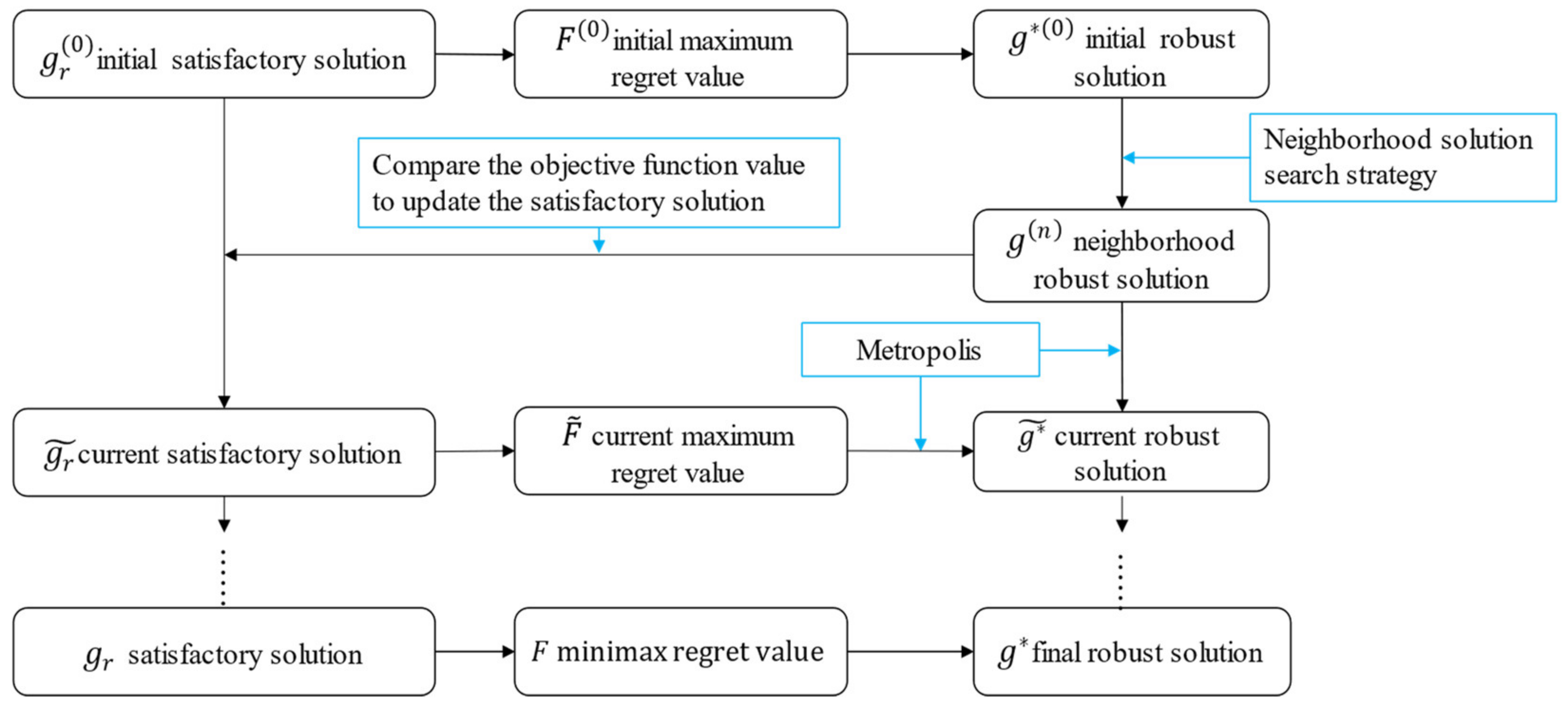
5. Simulated Annealing Algorithm Design

5.1. The Framework of the Designed Algorithm

The general train plan optimization problem has long been classified as a large-scale and complex NP-hard problem, and it is more difficult to solve the robust optimization problem of train plans that need to satisfy multiple demand scenarios. Considering that the simulated annealing algorithm has the advantages of strong search ability for new solutions, great applicability, and high degree of robustness, it has been proved to be able to effectively solve optimization problems of various types for train plans. Therefore, in this section, we will design a corresponding simulated annealing algorithm in accordance with the characteristics of the robust optimization problem for a train plan able to satisfy multiple demand scenarios.

As we know, the calculation of the maximum regret value is dependent on the optimal solution corresponding to each demand scenario. However, plenty of studies have shown that the calculation scale increases geometrically with increasing numbers of stations and trains. Usually, it is only possible to obtain an approximation of the optimal solution, and in this research this is referred to as the satisfactory solution for each demand scenario. Obviously, the maximum regret value calculated using the satisfactory solution for each demand scenario will not be accurate. To estimate the maximum regret value as accurately as possible in order to ensure the optimization quality of the robust solution during the iterative process, it is necessary not only to generate a robust neighborhood solution through continuous iteration on the basis of the initial robust solution, subsequently optimizing the robust solution, but also to improve the satisfactory solution for each demand scenario in combination with the updated robust solution. Thus, the simulated annealing algorithm framework was constructed as shown in Figure 4, with the specific process detailed in the following.

Firstly, an existing algorithm, which designed for the optimization of train plans for single-day demand in ref. [16], was used to obtain the satisfactory solutions under various demand scenarios. On the basis of this, the corresponding maximum regret value was calculated using the satisfactory solution for each demand scenario, and the satisfactory solution for a given demand scenario that corresponded to the minimax regret value was selected as the initial robust solution.

Before generating the neighborhood solution, it was necessary to evaluate the service level of each currently running train on the basis of the passenger flow assignment under each demand scenario. The overall idea of passenger flow assignment is as follows. Assuming that the generalized travel expense of each candidate train is known by all ODs, the train with the least expense will be chosen by all ODs. However, due to limitations such as train capacity, not all ODs are able to take the train with the least expense. When the number of passengers carried by the train in the rail section exceeds the train transportation capacity, after calculating the generalized travel expense of each candidate train again, the excess OD passenger flow needs to be transferred to other trains with the lowest relative travel expense and enough remaining capacity in the candidate train set, in order to minimize total passenger travel expense as much as possible, while guaranteeing that all passenger demand will be met. For the specific passenger flow assignment process, refer to Refs. [32,33].

Secondly, the service level of each train in the current robust solution was evaluated, and on this basis in combination with passenger travel choices under each demand scenario, the neighborhood solution was constructed. Then, for each demand scenario, it was checked and judged whether it was better to use the robust neighborhood solution that its corresponding satisfactory solution, and if so, the current satisfactory solution for that demand scenario was replaced with the robust neighborhood solution. Note that the construction of the robust neighborhood solution is the most critical innovation in this algorithm. Compared with existing methods for constructing neighborhood solutions only on the basis of single-day demand, this algorithm needs to be combined with passenger travel choices under multiple demand scenarios at the same time in order to adjust trains.

Next, the maximum regret value corresponding to the robust neighborhood solution was estimated using the updated satisfactory solution for each demand scenario, and this was compared with the maximum regret value of the current robust solution. Then, on the basis of the Metropolis criterion of the simulated annealing algorithm, it was judged whether to accept the robust neighborhood solution as the current robust solution.

Finally, the above process was repeated until the given algorithm termination conditions were met.

In the above algorithm framework, the initial robust solution can be generated directly using the existing train plan optimization method. Thus, the key innovation in this algorithm is the generation of the robust neighborhood solution search strategy. Next, we will introduce this search strategy, and the following contains the detailed steps of the algorithm.

5.2. Robust Neighborhood Search Strategy for Multiple Demand Scenarios

On the basis of the passenger flow assignment under each demand scenario and the evaluation of the service quality for each OD and each train, the following strategies were designed and implemented to update the current train plan.

(1)

Adjust the number of trains

Randomly delete some trains from the current train plan on the basis of the passenger seat rates of trains. Denote $L^{\prime }$ as the current number of trains and ${\alpha }_{max}$ as the maximum ratio of deleted trains. The ${\alpha }_{max}$ gradually decreases as the temperature drops during the solving process, so that the search range of the algorithm is wider during the early stages, while the algorithm converges faster during later stages. First, randomly generate a ratio $\alpha$, which must satisfy $\alpha \in \left(0,{\alpha }_{max}\right)$, and determine the current number of deleted trains as $L^{\prime }\times \alpha$. Then, on the basis of the passenger flow assignment, calculate the passenger seat rate ${\eta }_r^l$ for each train under each demand scenario, and take the average value of all demand scenarios as the train’s average passenger seat rate ${\eta }^l$. Finally, for each currently operating train, calculate the probability $p^{l-}=\left({\eta }_{max}-{\eta }^l\right)/{\displaystyle \sum }_{l\in L^{\prime } }\left({\eta }_{max}-{\eta }^l\right)$, where ${\eta }_{max}=\underset{l\in L^{\prime }}{\max }\left\{{\eta }^l\right\}$ is the maximum passenger seat rate of all of the trains, and then use this probability and the roulette method to select the $L^{\prime }\times \alpha$ trains to delete and release the passenger flow corresponding to each demand scenario.

For the released passenger flow in each demand scenario, firstly, try to distribute them among the operating trains with available capacity. In addition, for the biggest passenger flow that cannot be arranged, select the most suitable candidate trains that are not operating and calculate their average passenger seat rates. If this reaches the specified threshold, choose the train to operate. Any additional candidate trains will depart at the middle time of the maximum time gap in the time period, and the stops will be generated according to the stop mode of the train with the highest average passenger seat rate.

(2)

Adjust train stops

Randomly cancel some stops on the basis of the passenger flow and the stop frequency of each station. Denote $L_c$ as the current number of trains, ${\beta }_{max}$ as the ratio of cancelled stops. ${\beta }_{max}$ will gradually decrease as the temperature drops during the solving process. First, randomly generate the ratio $\beta$, which must satisfy $\beta \in \left(0,{\beta }_{max}\right)$, and determine the current number of cancelled stops as $L_c\times \beta$. Then, for stop $i$ of train $l$, calculate the passenger flow $Q_{l,i}^r$ and the number of trains $N_{l,i}^r$ serving passengers at stop $i$, and for $Q_{l,i}^r\times \left(1/N_{l,i}^r\right)$ of all demand scenarios, take the average value as $Q_{l,i}\times \left(1/N_{l,i}\right)$. Finally, calculate the probability $p^{-}{}_{l,i}=\left(Max-Q_{l,i}\times \left(1/N_{l,i}\right)\right)/{\displaystyle \sum }_{l\in L_c,i\in S_l}\left(Max-Q_{l,i}\times \left(1/N_{l,i}\right)\right)$, where $Max=\underset{l\in L_c,i\in S_l}{\max }\left\{Q_{l,i}\times \left(1/N_{l,i}\right)\right\}$, and then use these probabilities and the roulette method to select the stops that need to be cancelled. In addition, stops at which no passengers get on or off will be cancelled directly.

Meanwhile, randomly add some stops based on the passenger flow of the stop frequency of each station. Denote $L_c$ as the current number of trains, ${\mu }_{max}$ as the ratio of added stops. First, randomly generate the ratio $\mu$, which satisfies $\mu \in \left(0,{\mu }_{max}\right)$, and determine the current number of added stops as $L_c\times \mu$. Then, for the non-stop $i$ of the current train $l$, calculate the passenger flow $Q{\prime }_{l,i}^r$ and the number of trains $N{\prime }_{l,i}^r$ served for passengers at non-stop $i$, for $Q{\prime }_{l,i}^r\times \left(1/N{\prime }_{l,i}^r\right)$ of all demand scenarios, take the average value as $Q{\prime }_{l,i}\times \left(1/N{\prime }_{l,i}\right)$. Finally, calculate the probability $p^{+}{}_{l,i}=\left(Q{\prime }_{l,i}\times \left(1/N{\prime }_{l,i}\right)-Min\right)/{\displaystyle \sum }_{l\in L_c,i\in S_l}\left(Q{\prime }_{l,i}\times \left(1/N{\prime }_{l,i}\right)-Min\right)$, where $Min=\underset{l\in L_c,i\in S_l}{\min }Q{\prime }_{l,i}\times \left(1/N{\prime }_{l,i}\right)$, and then use these probabilities and roulette method to select stops that need to be added.

(3)

Adjust departure time of trains

Randomly select some trains to adjust their departure times according to the passenger departure time deviation. $L^{\prime }$ denotes the current number of trains, and ${\gamma }_{max}$ denotes the maximum adjustment ratio, which gradually decreases as the temperature drops. First, randomly generate the ratio $\gamma$, which must satisfy $\gamma \in \left(0,{\gamma }_{max}\right)$, and determine the current number of adjusted trains as $L^{\prime }\times \gamma$. Then, under each demand scenario, for any operation train $l^{\prime }$, calculate the total passenger departure time deviation, including early departure time $A^{l^{\prime }}$ and delayed departure time $D^{l^{\prime }}$. Finally, calculate the probability $p_{l^{\prime },t}=(A^{l^{\prime }}+D^{l^{\prime }})/{\displaystyle \sum }_{l^{\prime }\in L^{\prime }}(A^{l^{\prime }}+D^{l^{\prime }})$, and then use this probability and the roulette method to select some trains for which to adjust the departure times. If $A^{l^{\prime }}$ is greater than $D^{l^{\prime }}$, the departure time of the train will be advanced, otherwise it will be postponed.

5.3. Algorithm Steps

The relevant parameters in the simulated annealing schedule include: initial temperature ${\Psi }_0$, temperature drop ratio $\theta$, termination temperature ${\Psi }_{end}$, the upper limit of constant temperature iteration $U_{max}$, and number of iterations continuously keeping the optimal solution $\phi$. The algorithm termination condition is that the temperature drops to the termination temperature ${\Psi }_{end}$ or the maximum regret value does not change after $\phi$ iterations.

In summary, the simulated annealing algorithm for the robust optimization of train plan on the basis of multi-day demand scenarios is described in Algorithm 1.

Algorithm 1. Solving the robust optimization of train plan based on multi-day demand scenarios.

Input: High-speed railway line, candidate train set L, demand scenario set R, parameters of simulated annealing schedule.

Output: Robust solution g*, minimax regret value F.

Step1 Initialize parameter

Set the initial temperature value ${\Psi }_0$ the temperature drop ratio $\theta$ the termination temperature ${\Psi }_{end}$, the upper limit of constant temperature iteration $U_{max}$, and the number of iterations, continuously keeping the optimal solution $\phi$. Let the current temperature $\Psi ={\Psi }_0$, and the constant temperature iteration number n = 1.

Step2 Generate initial satisfactory solutions and initial robust solution

Apply the algorithm, solving train plan for single-day demand to generate initial satisfactory solution $g_r^{\left(0\right)}$ for each demand scenario r, and set the current satisfactory solution for each scenario as $\widetilde{g_r}=g_r^{\left(0\right)}$ the corresponding objective value is expressed as $Z^{r*}$. Take the current satisfactory solution for each demand scenario in turn as the robust solution, and calculate their corresponding maximum regret values; finally, choose the solution the corresponds to the minimax regret value $F^{\left(0\right)}$ as the initial robust solution $g^{*\left(0\right)}$. Further, set the current robust solution $\widetilde{g^{*}}=g^{*\left(0\right)}$, and set the current maximum regret value $\tilde{F}=F^{\left(0\right)}$.

Step3 Search robust neighborhood solution

Based on the current robust solution $\widetilde{g^{*}}$, allocate the passenger flow for each demand scenario to operating trains, then use the neighborhood solution search strategy detailed in Section 5.2 to generate a robust neighborhood solution $g^{\left(n\right)}$.

Step4 Update the satisfactory solution for each demand scenario

For any demand scenario, if the robust neighborhood solution $g^{\left(n\right)}$ causes $Z^{r*}>Z^r\left(g^{\left(n\right)}\right)$, update the satisfactory solution for the demand scenario $\widetilde{g_r}=g^{\left(n\right)}$, and set $Z^{r*}=Z^r\left(g^{\left(n\right)}\right)$; otherwise, keep the original satisfactory solution unchanged.

Step5 Judge whether to update the robust solution

Calculate the maximum regret value F′ of the robust neighborhood solution $g^{\left(n\right)}$, and compare it with the current maximum regret value $\tilde{F}$; next, implement the Metropolis criterion: (1) if $F^{\prime }<\tilde{F}$, accept the robust neighborhood solution $g^{\left(n\right)}$ as the current robust solution $\widetilde{g^{*}}$, and let $\tilde{F}=F^{\prime }$; (2) if $F^{\prime }>\tilde{F}$ and $exp\left[-\frac{\left(F^{\prime }-\tilde{F}\right)}{\Psi }\right]\ge rand\left(0,1\right)$ accept the robust neighborhood solution $g^{\left(n\right)}$ as the current robust solution $\widetilde{g^{*}}$, and let $\tilde{F}=F^{\prime }$; (3) otherwise, keep the current maximum regret value $\tilde{F}$ and the current robust solution $\widetilde{g^{*}}$ unchanged.

Step6 Check the number of iterations at the current temperature

If $n=U_{max}$, then drop the temperature, set $\Psi =\Psi \times \theta$, and n = 1; otherwise, set the number of constant temperature iterations n = n + 1, and go to Step 3.

Step7 Check termination condition

If $\Psi <{\Psi }_{end}$ or the current maximum regret value $\tilde{F}$ does not change in $\phi$ iterations, terminate the algorithm and output the final robust solution $g^{*}$; otherwise, let n = 1 and go to Step 3.

6. Experiments and Results

In this section, using the Shijiazhuang–Jinandong high-speed railway corridor in China as an example, a series of computational experiments are carried out to verify the effectiveness of the proposed robust optimization method.

The physical network of the Shijiazhuang–Jinandong high-speed railway corridor is shown in Figure 5. It has a total length of 323 km and has 11 stations, including two endpoint stations and nine intermediate stations; the distances between the stations are 20 km, 23 km, 33 km, 46 km, 48 km, 42 km, 26 km, 20 km, 30 km and 35 km, respectively.

We only optimize the train plan from Shijiazhuang to Jinandong in the downward direction. The range of travel departure times of passengers throughout the day is from 06:00 to 23:00, which is divided into 17 time periods with a length of 1 h. Take the passenger demand for weekdays as the demand scenario set, and select the demand over five days, for which the total number of passengers were 93,967, 91,197, 94,667, 92,433, and 90,563, respectively.

Because Shijiazhuang station and Jinandong station are the stations corresponding to the points of original departure and final arrival of trains on the Shi-Ji high-speed railway line, they are used as the origin–destination stations of each candidate train. To meet passenger demand in each time period on each operation day, the method introduced in Section 3.2 is used to generate the candidate train set that adapts to multi-day demand scenarios. For example, during the period 16:00~17:00, the passenger flow under demand scenario 4 is the highest, so 11 candidate trains need to be arranged for this period, as determined using the formula for calculating the number of candidate trains. By analogy, on the basis of the number of candidate trains that need to be arranged for each time period, it can be obtained that there will be 110 trains throughout the day.

The parameters related to the simulated annealing algorithm are shown in

Table 2. The parameters related to simulated annealing algorithm.

Parameter	Value
Initial temperature	10,000 °C
End temperature	100 °C
Maximum iterations at constant temperature	30
Cooling rate	0.9
Number of iterations continuously keeping the optimal solution	600

, and the parameters related to train operation are shown in

Table 3. The parameters related to train operation.

Parameter	Value
Fixed organizational cost of train operation	4000 Ұ/train
Operation cost per unit travel time of train	150 Ұ/min
Train capacity	946 seats
Stop time at each station (including additional starting and braking time)	intermediate station: 3 min departure and arrival station: 7 min
Train fare rate per person-kilometer 1	0.42 Ұ/km
Passenger unit time value coefficient	37.8 Ұ/h [16]
Train speed	250 km/h
Maximum capacity of passing through each rail section during each time period	10 pairs/h
Maximum train departure interval of service for OD 2	peak hours: 45 min other hours: 70 min

¹ The train fare rate per person-kilometer can be calculated according to the ratio of the number of seats of different seats and the intensity of passenger flow (person/km); ² From analysis of the passenger flow demand on the Shijiazhuang–Jinan high-speed rail line, we know that the peak travel time of most operation days is 8:00~10:00 and 15:00~17:00.

.

6.1. Sensitivity Analysis

Obviously, if there are more operating trains, passengers have more trains available on which to travel, which can shorten their travel time and reduce their travel cost, but the train operation cost will increase accordingly. Conversely, with fewer operating trains, although railway enterprises will enjoy low operation costs, passengers will receive a bad service. Thus, in order to better balance these two aspects, we assign weights to the train operation cost and passenger travel expense, respectively, and explore the impact of these weight values on the train plan.

Firstly, the value range [0, 1] is assigned to weight $\omega$, with an interval of 0.1. A sensitivity analysis is carried out for all demand scenarios, and the average value of the two indicators is obtained in order to describe the change curve of train operation cost and passenger travel expense with $\omega$, as shown in Figure 6. With increasing $\omega$, the weight of the train operation cost gradually increases. During the optimization process, the train operation cost generally shows a decreasing trend; while the weight of the passenger travel expense gradually decreases, the indicator shows an increasing trend. However, when $\omega$ = 0.3, the two indicators are both at a low level, which can be considered to reflect the minimization of both indicators. Therefore, it is reasonable for the weight to take a value of 0.3, which is able to provide better service quality for passengers while also not causing the train operation cost to increase too far.

6.2. Results Analysis

The above example is solved using a computer with a memory of 16 GB and a CPU consisting of 4 cores, and was implemented in the MATLAB R2018a program. At first, it took about 1000 s to find a satisfactory solution for each demand scenario. Taking demand scenario 1 as an example, the convergence process to find a satisfactory solution is shown in Figure 7. The iteration time for solving the robust solution was 5579 s. The convergence process of the minimax regret value is shown in Figure 8. When approaching the number of iterations $\phi$ after which optimal solution remains continuous, the curve tends to eventually become stable, thus proving that the algorithm has achieved excellent convergence performance.

Table 4. Comparison between the robust scheme and the satisfactory scheme for each demand scenario.

Demand Scenario	Trains	Total Objective/Ұ	Train Operation Cost/Ұ	Passenger Travel Expense/Ұ	Maximum Deviation between Robust and Satisfactory Scheme/Ұ	Maximum Deviation Percentage
1	74	8,490,938	1,511,300	11,482,211	\	\
Robust	80	8,578,625	1,532,900	11,598,221	87,687	1.03%
2	71	8,138,830	1,443,500	11,008,257	\	\
Robust	80	8,311,165	1,532,900	11,216,135	172,335	2.12%
3	75	8,399,025	1,533,000	11,341,607	\	\
Robust	80	8,635,289	1,532,900	11,679,170	236,264	2.81%
4	77	8,358,884	1,584,050	11,262,384	\	\
Robust	80	8,532,729	1,532,900	11,532,656	173,845	2.08%
5	80	8,280,392	1,543,700	11,167,545	\	\
Robust	80	8,320,424	1,532,900	11,229,363	40,032	0.48%

presents a comparison of the total objective, train operation cost and passenger travel expense when implementing the satisfactory train plan with those when implementing the robust train plan for each demand scenario. The maximum regret value converges from the initial value of 4,785,241 to 236,264, and the deviation gradually shrinks, so that the maximum deviation percentage is 2.81% (marked in red color). This indicates that during the optimization process, the robust solution approaches the satisfactory solution for each demand scenario as closely as possible.

Figure 9 presents the robust train plan generated for five demand scenarios, and includes basic information such as train origin and destination, number of trains, stop plan, and departure time. There are a total of 80 trains from Shijiazhuang to Jinandong in the train plan, including 3 nonstop trains and 77 trains with alternate stops. There are 21 trains only stopping at large-scale stations such as Shijiazhuangdong station, Hengshuibei station or Dezhoudong station. The use of nonstop trains and trains stopping at large-scale stations ensures that the travel efficiency of ODs with plenty of passenger demand remains at a high level.

To analyze the effect of the robust train plan implemented on each operation day, the following three implementation situations were considered: firstly, the train plan was independently generated and implemented according to passenger demand on each operation day, denoted as $S_{best}$; secondly, these satisfactory schemes were implemented on all operation days, respectively, denoted as $S_1,S_2,\cdots S_5$; thirdly, the robust train plan obtained in this paper was implemented on all operation days, denoted as $S_{robust}$. The average values of the indicators corresponding to the three implementation situations are shown in

Table 5. Comparison of indicators under the three implementation scenarios.

Scheme	Trains	Average Maximum Regret Value/Ұ	Average Total Objective/Ұ	Average Train Operation Cost/Ұ	Average Passenger Travel Expense/Ұ	Average Stop Frequency
$S_{best}$	76	\	8.334 × 106	1.523 × 106	1.125 × 107	6.0
$S_{robust}$	80	1.420 × 105	8.476 × 106	1.533 × 106	1.145 × 107	5.0
$S_1$	74	3.680 × 105	8.702 × 106	1.511 × 106	1.178 × 107	6.2
$S_2$	71	1.554 × 105	8.489 × 106	1.444 × 106	1.151 × 107	5.9
$S_3$	75	2.701 × 105	8.604 × 106	1.533 × 106	1.163 × 107	6.2
$S_4$	77	4.374 × 105	8.771 × 106	1.584 × 106	1.185 × 107	6.5
$S_5$	80	1.480 × 105	8.482 × 106	1.543 × 106	1.146 × 107	5.3

Note: average maximum regret value, average total objective, average train operation cost, and average passenger travel expense to four significant digits.

. The results show that if a train plan is selected from among the satisfactory schemes for all demand scenarios and implemented on all operation days, the total objective value and average maximum regret value will be larger than for the robust train plan (marked with red color in Table 5). This proves that the robust train plan is able to more effectively satisfy multi-day demand than the satisfactory scheme generated by independent optimization of each demand scenario. In addition, the average stop frequency when the robust train plan is lower than in the satisfactory solution, thus shortening passenger travel time, improving service quality for passengers, and reducing train operation cost.

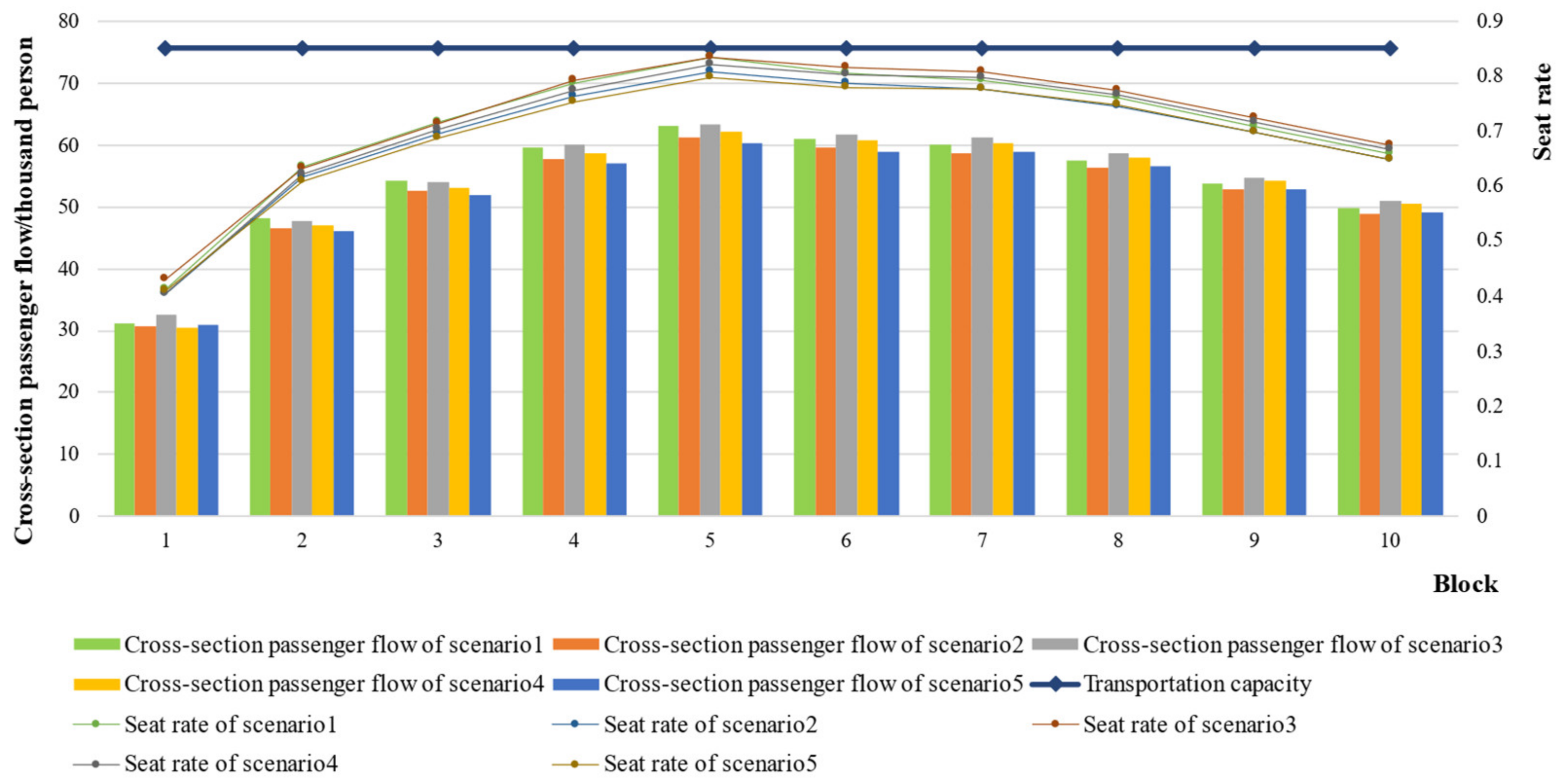
6.3. Analysis of the Matching of Train Operation with Demand for Each Day

Figure 10 displays the matching between the number of trains and OD passenger flow for each time period. During the periods 9:00~11:00 and 15:00~17:00, passenger flow was relatively high, and the number of trains reached 7 to 8, accordingly. In other periods, the passenger flow was relatively low, so the number of trains was reduced, accordingly. This shows that the robust train plan is able to make the number of trains in each time period effectively match the passenger demand in that time period. It should be noted that due to the comprehensive consideration of the operation cost incurred by rail enterprises as well as the supply of train services to passengers, no trains were arranged for some of the OD demand during the time period from 22:00 to 23:00. This is because if we operate some trains during this time period, then the incurred operation cost will be greater than the travel cost saved by passengers traveling using these trains compared with when traveling in advance.

Figure 11 depicts the correspondence between passengers getting on and off and the number of stops at each station. Among the stations through which the trains pass, there are many passengers getting on and off at Shijiazhuangdong station, Xinjinan station, Hengshuibei station and Dezhoudong station, and therefore more trains should stop at these stations. The number of trains serving these stations accounts for about 50% of the total number of trains. Because the passenger flow for Gaochengnan station, Pingyuandong station and Qihe station are relatively lower, correspondingly fewer trains stop at those stations, but still more than 20 trains, thus ensuring that the intervals of trains serving the passenger flows of these stations meet the constraint.

Figure 12 displays the transportation capacity, cross-section passenger flow, and average seat rate for each rail section under each demand scenario. The rail section with the peak transportation volume is that from Xinjinan station to Pingyuandong station. This rail section passes through Hengshuibei station and Dezhoudong station, which have higher passenger flows, so the seat rate is about 80%, and the seat rate of most of the rail sections is above 70%. Therefore, the train transportation capacity is well utilized under each demand scenario in the robust train plan.

Figure 13 displays the passenger departure time deviation for each time period under each demand scenario. Among them, the average passenger departure time deviations under the five demand scenarios (indicated by the red solid line) were, respectively, 16.04 min, 15.45 min, 15.60 min, 17.87 min, and 18.17 min. It can be seen that the departure time deviation in most time periods was below the average value. Especially in time period 11, which had the largest passenger demand, the deviation values were lower than the average values under all demand scenarios, and were only 10.23 min in scenario 5, indicating that the departure times of trains in peak hours conformed to passengers’ expectations. Because the robust train plan must consider the space–time distribution of passenger flow in each demand scenario, there are some differences in meeting passengers’ demand for specific departure times. For example, the departure time deviation in time period 15 exceeds the average value and is close to 40 min in scenarios 4 and 5, while it is below the average value in other demand scenarios. This suggests that the matching degree of trains in time period 15 for demand scenarios 4 and 5 needs to be improved.

6.4. Analysis of the Number of Demand Scenarios Influencing Robust Optimization

With the expansion of the scale of the demand scenarios, the train plan and its indicators obtained by the robust optimization method will inevitably change. It is necessary to verify whether the proposed robust optimization method for train plans has general applicability. Five demand scenarios were added, with total demand of 89,427, 92,530, 95,177, 89,964, and 96,338, respectively. The robust scheme under each demand scale scenario was solved by progressively increasing the number of scenarios, and the maximum regret value was obtained in order to explore the change in deviation between the robust scheme and the satisfactory scheme for each demand scenario.

Table 6. The maximum deviation value and maximum deviation percentage between the robust scheme and the satisfactory scheme under each scale of the demand scenarios.

Scale of Demand Scenarios/Sort	Trains	Maximum Deviation/Ұ	Maximum Deviation Percentage/%
5	80	236,264	2.81
6	78	184,691	2.26
7	83	257,655	3.07
8	78	288,660	3.53
9	84	263,131	3.14
10	79	300,879	3.66

shows the maximum deviation value and maximum deviation percentage between the robust scheme and the satisfactory scheme under each scale of the demand scenarios. With increasing numbers of scenarios, the robust scheme needs to adapt to the fluctuations in the total number and space–time distributions of these demand scenarios, so it is more complicated to adjust the number of trains, stop plans, etc., and the maximum deviation between the robust scheme and the satisfactory scheme is more obvious. However, in terms of the maximum deviation percentage, the difference between the two remains in an acceptable range, and the maximum deviation value does not tend to increase infinitely. This demonstrates that the robust optimization method for train plans proposed in this paper has great general applicability.

7. Conclusions

In this paper the robust optimization problem of high-speed railway train plans was studied in light of passenger demand for multiple operation days. By adjusting the number of trains, the stop plan, and the departure time, passenger demand on each operation day could be effectively met, and train operation efficiency could be guaranteed. The main contributions and conclusions are as follows:

(1)

By regarding the passenger demand on each day as a demand scenario, we constructed a generation strategy for a candidate train set adapted to multi-day demand scenarios in order to provide support for solving the problem of the robust optimization of train plans.

(2)

The regret value was used to measure the deviation of total cost, including train operation cost and passenger travel expense, generated by the robust and optimal train plan for each demand scenario. Then, a robust optimization model of train plans for multi-day demand scenarios was constructed with the aim of minimizing the maximum regret value, and a corresponding simulated annealing algorithm was designed to solve the robust optimization model based on the construction of the robust neighborhood solution search strategy for multi-demand scenarios.

(3)

The Shijiazhuang–Jinandong high-speed railway line was used to verify the efficiency of the model and algorithm. The results showed that the maximum deviation percentage was 2.81% when the robust scheme was implemented on all operation days compared to when the satisfactory scheme was implemented on each operation day, so the robust scheme gradually became close to the satisfactory scheme for each scenario. In addition, if one of the satisfactory schemes were randomly selected for implementation in all demand scenarios on all operation days, the total costs would be larger than those for the robust scheme. It was proved that the robust scheme is able to effectively satisfy different demand scenarios of multiple operation days, and that the proposed robust optimization method for train plans is both valid and feasible.

The following three aspects can be regarded as the focus of our future research.

(1)

The type of train and the transfer of OD in the high-speed railway network are not currently considered. Future work should focus on the robust optimization study of the train plan of high-speed railway networks, taking the transfer of cross-line passenger flow into consideration.

(2)

It is possible to combine the train plan with the timetable to perform coordinated robust optimization in the case of train delays.

(3)

In the study of robust optimization, this paper only considers different passenger demand scenarios on multiple days, but there are many random factors affecting the train operation process. We should consider a variety of different factors as comprehensively as possible to make the model closer to the actual situation.

References

1. Park, B.H.; Seo, Y.I.; Hong, S.P.; Rho, H.L. Column generation approach to line planning with various halting patterns—Application to the korean high speed railway. Asia Pac. J. Oper. Res. 2013, 30, 1–19. [Google Scholar] [CrossRef]
2. Zeng, Q.; Deng, L.B.; Gao, W.; Zhou, W. Optimization Method for Train Plan of Urban Rail Transit with Elastic Demands. In Proceedings of the 12th International Conference of Transportation Professionals (CICTP 2012), Beijing, China, 3–6 August 2012; pp. 1770–1781. [Google Scholar] [CrossRef]
3. Su, H.; Tao, W.; Hu, X. A line planning approach for high-speed rail networks with time-dependent demand and capacity constraints. Math. Probl. Eng. 2019, 2019, 7509586. [Google Scholar] [CrossRef]
4. Zhao, S.; Wu, R.F.; Shi, F. A line planning approach for high-speed railway network with time-varying demand. Comput. Ind. Eng. 2021, 160, 107547. [Google Scholar] [CrossRef]
5. Claessens, M.T.; Dijk, N.M.V.; Zwaneveld, P.J. Cost optimal allocation of rail passenger lines. Eur. J. Oper. Res. 1998, 110, 474–489. [Google Scholar] [CrossRef]
6. Goosuerw, J.W.H.M. Models and Algorithms for Railway Line Planning Problems; Universiteit Maastricht: Maastricht, The Netherlands, 2004. [Google Scholar]
7. Fu, H.; Nie, L.; Meng, L.; Sperry, B.R.; He, Z. A hierarchical line planning approach for a large-scale high speed rail network: The China case. Transp. Res. Part A 2015, 75, 61–83. [Google Scholar] [CrossRef]
8. Liu, Y.; Cao, C. A multi-objective train operational plan optimization approach for adding additional trains on a high-speed railway corridor in peak periods. Appl. Sci. 2020, 10, 5554. [Google Scholar] [CrossRef]
9. Yan, F.; Goverde, R. Combined line planning and train timetabling for strongly heterogeneous railway lines with direct connections. Transp. Res. Part B Methodol. 2019, 127, 20–46. [Google Scholar] [CrossRef]
10. Zhang, C.T.; Qi, J.G.; Gao, Y.; Yang, L.; Gao, Z.; Meng, F. Integrated optimization of line planning and train timetabling in railway corridors with passengers’ expected departure time interval. Comput. Ind. Eng. 2021, 162, 1–22. [Google Scholar] [CrossRef]
11. Yue, Y.; Wang, S.; Zhou, L.; Tong, L.; Saat, M.R. Optimizing train stopping patterns and schedules for high-speed passenger rail corridors. Transp. Res. Part C Emerg. Technol. 2016, 63, 126–146. [Google Scholar] [CrossRef]
12. Jiang, F.; Cacchiani, V.; Toth, P. Train timetabling by skip-stop planning in highly congested lines. Transp. Res. Part B Methodol. 2017, 104, 149–174. [Google Scholar] [CrossRef]
13. Dong, X.; Li, D.; Yin, Y.; Ding, S.; Cao, Z. Integrated optimization of train stop planning and timetabling for commuter railways with an extended adaptive large neighborhood search metaheuristic approach. Transp. Res. Part C Emerg. Technol. 2020, 117, 102681. [Google Scholar] [CrossRef]
14. Barrena, E.; Canca, D.; Coelho, L.C.; Laporte, G. Single-line rail rapid transit timetabling under dynamic passenger demand. Transp. Res. Part B Methodol. 2014, 70, 134–150. [Google Scholar] [CrossRef]
15. Li, X.; Li, D.; Hu, X.; Yan, Z.; Wang, Y. Optimizing train frequencies and train routing with simultaneous passenger assignment in high-speed railway network. Comput. Ind. Eng. 2020, 148, 106650. [Google Scholar] [CrossRef]
16. Zhou, W.L.; Liu, X.H.; Jiang, M. Optimization of train plan on intercity railway based on candidate train set and elastic demand. J. China Railw. Soc. 2020, 42, 1–10. [Google Scholar] [CrossRef]
17. Lin, B.L.; Zhao, Y.N.; Lin, R.; Liu, C. Integrating traffic routing optimization and train formation plan using simulated annealing algorithm. Appl. Math. Model. 2021, 93, 811–830. [Google Scholar] [CrossRef]
18. Kouvelis, P.; Yu, G. Robust Discrete Optimization and Its Applications; Springer: Boston, MA, USA, 1997. [Google Scholar] [CrossRef]
19. Mulvey, J.M.; Vanderbei, R.J.; Zenios, S.A. Robust optimization of large-scale systems. Oper. Res. 1995, 43, 264–281. [Google Scholar] [CrossRef] [Green Version]
20. Hassannayebi, E.; Zegordi, S.H.; Amin-Naseri, M.R.; Yaghini, M. Train timetabling at rapid rail transit lines: A robust multi-objective stochastic programming approach. Oper. Res. 2016, 17, 435–477. [Google Scholar] [CrossRef]
21. Pu, S.; Wang, W.X.; Chen, D.J.; Lv, H.X. The robust model for line planning problems of high-speed passenger train. J. Transp. Syst. Eng. Inf. Technol. 2015, 15, 105–110. [Google Scholar] [CrossRef]
22. Jamili, A.; Aghaee, M.P. Robust stop-skipping patterns in urban railway operations under traffic alteration situation. Transp. Res. Part C Emerg. Technol. 2015, 61, 63–74. [Google Scholar] [CrossRef]
23. Sun, H.J.; Cai, Z.Q.; Peng, C.H. Robust optimization model for passenger transport line planning considering the uncertain passenger flow. J. East China Jiaotong Univ. 2016, 33, 83–90. [Google Scholar] [CrossRef]
24. Cacchiani, V.; Qi, J.G.; Yang, L.X. Robust optimization models for integrated train stop planning and timetabling with passenger demand uncertainty. Transp. Res. Part B 2020, 136, 1–29. [Google Scholar] [CrossRef]
25. Assavapokee, T.; Realff, M.J.; Ammons, J.C. Min-max regret robust optimization approach on interval data uncertainty. Optim. Theory Appl. 2008, 137, 297–316. [Google Scholar] [CrossRef] [Green Version]
26. Bell, D.E. Regret in decision making under uncertainty. Oper. Res. 1982, 30, 961–981. [Google Scholar] [CrossRef]
27. Ning, C.; You, F. Adaptive robust optimization with minimax regret criterion: Multi-objective optimization framework and computational algorithm for planning and scheduling under uncertainty. Comput. Chem. Eng. 2018, 108, 425–447. [Google Scholar] [CrossRef]
28. Ye, Z.F. Research on the reliability of decision-making goals and results of uncertain decision-making methods. J. Ind. Eng. Eng. Manag. 2000, 14, 59–61. [Google Scholar] [CrossRef]
29. Zhou, L.; Yang, X.; Wang, H.; Wu, J.; Chen, L.; Yin, H.; Qu, Y. A robust train timetable optimization approach for reducing the number of waiting passengers in metro systems. Phys. A Stat. Mech. Its Appl. 2020, 558, 124927. [Google Scholar] [CrossRef]
30. Qu, Y.C.; Wang, H.; Wu, J.; Yang, X.; Yin, H.; Zhou, L. Robust optimization of train timetable and energy efficiency in urban rail transit: A two-stage approach. Comput. Ind. Eng. 2020, 146, 106594. [Google Scholar] [CrossRef]
31. Fu, H.L.; Nie, L.; Yang, H.; Tong, L. Research on the method for optimization of candidate-train-set based on train operation plans for high-speed railways. J. China Railw. Soc. 2010, 32, 1–8. [Google Scholar] [CrossRef]
32. Huang, Z.P.; Zhang, Y.Z.; Zhang, Z.; Yang, L. Optimization of train timetables in high-speed railway corridors considering passenger departure time and seat-class preferences. Transp. Lett. 2022, 1–18. [Google Scholar] [CrossRef]
33. Lin, D.Y.; Fang, J.H.; Huang, K.L. Passenger assignment and pricing strategy for a passenger railway transportation system. Transp. Lett. 2019, 6, 320–331. [Google Scholar] [CrossRef]
Figure 1. The distribution of daily passenger demand at Jingzhou station over two months.
Mathematics 10 01278 g001
Figure 2. The fluctuation of the same OD passenger flow on each operation day.
Mathematics 10 01278 g002
Figure 3. The diagram of a candidate train set generation for a given period.
Mathematics 10 01278 g003
Figure 4. The algorithm of the designed framework.
Mathematics 10 01278 g004
Figure 5. Map of the Shi-Ji high-speed railway line.
Mathematics 10 01278 g005
Figure 6. Graph of the sensitivity analysis.
Mathematics 10 01278 g006
Figure 7. Convergence graph of all indicators under scenario 1.
Mathematics 10 01278 g007
Figure 8. Convergence graph of maximum regret value.
Mathematics 10 01278 g008
Figure 9. The train plan of Shi-Ji high-speed railway in the downward direction.
Mathematics 10 01278 g009
Figure 10. Matching between the number of trains and OD passenger flow during each time period.
Mathematics 10 01278 g010
Figure 11. Correspondence between the train stops at each station and passengers getting on and off.
Mathematics 10 01278 g011
Figure 12. Transportation capacity, cross-section passenger flow, and average seat rate of each rail section under each demand scenario.
Mathematics 10 01278 g012
Figure 13. The passenger departure time deviation in each time period under each demand scenario.
Mathematics 10 01278 g013