Estimating Scattering Potentials in Inverse Problems with a Non-Causal Volterra Model

Abstract

In this paper, a finite memory, non-causal Volterra model is proposed to estimate the potential functions in various inverse quantum mechanical problems, where the bound or scattered wave functions are used as inputs of the Volterra system, while the potential is the desired output. Two simple examples are given to show the model capabilities, where in both cases, a really good match is achieved for a very wide range of potential functions. The first example is a simple one-dimensional bound state problem, where the wave function of the first bound state is used as input to determine the model potential. The second example is a one-dimensional scattering problem, where the scattered wave is used as the system input. In both cases, a higher order, non-causal description is needed to be able to give a good estimation to the solution of the inverse problem. The model sensitivity to input perturbations is also examined, showing that the Volterra representation is capable of giving a robust estimate to the underlying dynamical system. The model could be useful in real-life situations, where the scattering potential should be found from measured data, where the precise equations that govern the dynamics of the system are not known.

1. Introduction

Inverse problems are a really important subset of problems in both classical and quantum systems, where one is concerned with the determination of some input parameters, functions, and/or some inner characteristics of a complex system, with using only the output of the general system. These kinds of problems are present in many topics from engineering, e.g., in robotics [1,2], in thermal inverse problems [3], in the determination of material properties [4], etc. to nuclear physics, where usually an unkown potential has to be determined from experimental data [5,6,7,8]. In most of the cases, these problems are mathematically ill-defined, and the method of solution usually depends on the actual problem, the measurement methods, and the a priori knowledge of the system considered. For quantum mechanical problems, a well-known inversion method is the Gelfand-Levitan and Marchenko technique [9,10,11], which is an exact integral approach for Schrödinger-like equations that have many applications in quantum scattering theory. Other integral-based methods similiar to the Gelfand-Levitan and Marchenko equations are also developed for various kinds of problems [12,13,14,15].

In this paper, only simplified inverse quantum mechanical problems are addressed, where the output wave functions (bound states, scattering states) are used to determine the model potential; however, the model can be extended to describe “classical” inverse and non-inverse problems as well. Here, the inverse problem is not solved exactly; instead, an approximate method is used to give the solution to the actual problem in the least squares sense. To this purpose, the quantum mechanical problem is modeled as a non-causal gray-box system, which is identified with standard system identification techniques [16]. Then, the system is modeled with a finite-memory Volterra representation [17], which is capable of grasping various kinds of static and dynamic nonlinearities in a dynamical system described by nonlinear differential equations. This method is very general and can be used for other kinds of direct and inverse problems as well [18,19]. In the system identification of real-life physical systems, usually, a causal representation is used, which means that the dynamical response of the system $y\left[t\right]$ only depends on the actual and the previous values of the excitations, e.g., $y\left[t\right]=F\left(u\right[t],u[t-\mathsf{\Delta }t],u[t-2\mathsf{\Delta }t],$…$u[t-N\mathsf{\Delta }t])$. In contrast, non-causal systems are systems where the output at point t could depend not just on the previous but also the future values of the excitation signals as well, e.g., $y\left[t\right]=F\left(u\right[t],u[t-\mathsf{\Delta }t],$…$u[t-N\mathsf{\Delta }t],u[t+\mathsf{\Delta }t],u[t+2\mathsf{\Delta }t],$…$u[t+M\mathsf{\Delta }t])$, where $y\left[t\right]$ is the output, and $u\left[t\right]$ is the input at point t, which can be time, position, or any variable, on which the input and output functions depend. Non-causal systems can be used in post-processing of sound files, filtering, or image processing, where the pixels of an image can be considered as the variables of the input function [20]. Here, the notions of “past” and “future” are used loosely, as they do not exclusively represent time but rather can represent anything on which the input and output functions depend. In the applications shown in this paper, it turned out that a non-causal description is needed to be able to describe the inverse problem with a good accuracy, where to determine the potential at position x, the local information of the output wave function at points ($x+\mathsf{\Delta }x,x+2\mathsf{\Delta }x,$…$x+M\mathsf{\Delta }x,x,x-\mathsf{\Delta }x,x-2\mathsf{\Delta }x,$…$,x-M\mathsf{\Delta }x$) are used as inputs of the Volterra system. The problems shown here are very simple and are only used to present the method and its capabilities; however, as the model is very flexible, it is possible to extend it to be able to describe real-life systems, e.g., low-energy elastic scattering in nuclear physics, where the measured phase-shifts and differential cross-sections could be used as input data to estimate the potentials. These problems will be addressed in subsequent works. In quantum mechanics, despite its capabilities to describe nonlinear and complex systems, non-causal Volterra series are not extensively used to describe the direct or inverse problems. This work is intended to introduce the Volterra approximation to quantum mechanical systems, and it could lead to many more applications, from tunneling experiments, through low-energy nucleus scattering, up to high-energy hadronic scattering.

The paper is organized as follows. In Section 2, the Volterra model is introduced, which is used to describe the inverse quantum mechanical scattering system. Following the description of the system identification method, in Section 3, the first example is shown, where the one-dimensonal bound state problem is addressed. In Section 4, the Volterra model is used to describe the inverse scattering problem in one dimension, while Section 5 deals with the sensitivity of the Volterra model to input disturbations. At the end, Section 6 concludes the paper.

2. Volterra Model

The Volterra model is a well-known method to represent nonlinear dynamical systems and has a very wide range of applicability from identifying the behavior of electronic devices, such as field effect transistors [21] through the description of biological systems [22], all the way to mechanical engineering, aerospace engineering, and many more real-life problems [23,24]. The model extends the usual linear response theory, where the output of a linear dynamical system can be described by the convolutional integral of the input signal with a $h\left(t\right)$ kernel function as:

$$y\left(t\right)={\int }_{-\infty }^{\infty }h\left(\tau \right)u(t-\tau )d\tau ,$$

(1)

where $y\left(t\right)$ is the output and $u\left(t\right)$ is the input of the system, while $h\left(t\right)$ is the so-called linear response, which acts as the kernel function, which characterizes the system. For linear systems, this description is enough to describe the output; however, many real-life problems have more or less nonlinearities hidden in them, which could easily make the identified linear model practically unusable. For weakly nonlinear systems, the so-called best linear approximation (BLA) [25] is often used, which finds the best linearization of the nonlinear system in a specific operating range in the least squares sense, which can be expressed as the following optimization problem:

$$g_{BLA}\left(t\right):=\arg {\min }_g\mathcal{E}\left[{\left(y-{\int }_{-\infty }^{\infty }g\left(\tau \right)u(t-\tau )d\tau \right)}^2\right],$$

(2)

where $g_{BLA}$ is the linear kernel, which describes the weakly nonlinear input–output relation in the best way possible in the least squares sense. For the sake of generality, the convolutional integral goes from $-\infty$ to $\infty$; however, if one has a strictly causal system, then it goes from 0 to $\infty$. This method works really well in many applications; however, if the system has a stronger nonlinearity or the operating range is wider than what the simple linear approximation can describe, it is necessary to use different methods.

The Volterra model is an extension of the linear theory to nonlinear systems, where the input–output relation of a system of order n is described by a multidimensional convolutional integral descibed as follows [26,27]:

$$\begin{array}{cc}\hfill y\left(t\right)& =h_0+{\int }_{-\infty }^{\infty }{h}_1\left({\tau }_1\right)u(t-{\tau }_1)d{\tau }_1+{\int }_{-\infty }^{\infty }{\int }_{-\infty }^{\infty }{h}_2({\tau }_1,{\tau }_2)u(t-{\tau }_1)u(t-{\tau }_2)d{\tau }_{1}d{\tau }_2+\hfill \\ \hfill & +\dots +{\int }_{-\infty }^{\infty }\dots {\int }_{-\infty }^{\infty }{h}_n({\tau }_1,\dots ,{\tau }_n)u(t-{\tau }_1)\dots u(t-{\tau }_n)d{\tau }_1\dots d{\tau }_n,\hfill \end{array}$$

(3)

where $h_n({\tau }_1,\dots ,{\tau }_n)$ is the n-th order Volterra kernel, $y\left(t\right)$ is the output, while $u\left(t\right)$ is the input of the system at t. This can be written in a more compact form if one defines the n-th order Volterra operator as $H_n\left[u\left(t\right)\right]$ as:

$$H_n\left\{u\left(t\right)\right\}={\int }_{-\infty }^{\infty }\dots {\int }_{-\infty }^{\infty }{h}_n({\tau }_1,\dots ,{\tau }_n)u(t-{\tau }_1)\dots u(t-{\tau }_n)d{\tau }_1\dots d{\tau }_n,$$

(4)

so that Equation (3) can be written as:

$$y\left(t\right)=h_0+H_1\left\{u\left(t\right)\right\}+H_2\left\{u\left(t\right)\right\}+\dots +H_n\left\{u\left(t\right)\right\}$$

(5)

In the Volterra representation in Equation (3), it was implicitly assumed that the kernels are stationary, which means that the kernel functions depend only on the difference ($t-{\tau }_i$); therefore, the n-th order kernel can be written as $h_n({\tau }_1,\dots ,{\tau }_n)$ [28]. In the case that the kernels are non-stationary [29], they explicitly depend on t and can be written as $h_n(t,{\tau }_1,\dots ,{\tau }_n)$. In this work, only stationary kernels are assumed.

In many physical systems, the input–output relationship is hereditary, which means that the output at a specific instant $t_0$ depends on the input excitation on that instant and also on its values before $t_0$. In linear systems this behaviour is encoded into the convolutional integral in Equation (1), however in nonlinear systems the hereditary property [30] can be described by a multidimensional convolutional integral as it was shown in Equation (3). In this case the output at a specific instant is described by polynomial expressions of the input excitations at different $t_i$-s. One important application of such representations is in control engineering, where the (non)linear system has to be controlled in an open- or in a closed loop to reach the desired behaviour [31]. If the system or the controller is nonlinear it is necessary to include nonlinear terms into the model, e.g., in [32,33]. In the case of Volterra operator-integral equations, appearing in the feedback control problems using Volterra models [34], the convergence of the approximations can be studied by the majorant method [35].

In the Volterra representation, the $h_n({\tau }_1,\dots {\tau }_n)$ kernel functions are playing the most important role and have to be defined to be able to model the nonlinear system. If the system is known precisely, it can be calculated analytically; however, it is rarely the case, and those models are mostly used to validate the different methods used for kernel estimation [36]. Measuring the kernel functions is quite cumbersome, and in practical applications, a finite memory approximation is used where the kernel functions are truncated to a finite memory M, so that $h_n({\tau }_1,\dots ,{\tau }_n)$ = 0 if ${\tau }_i>M$ for $i=1\dots n$. This procedure can be extended to non-causal systems as well where the kernels are vanishing if $|{\tau }_n|>M$. As it was noted, measuring the kernels is quite the cumbersome task, and there are many different methods to do it. The simplest one would be to discretize Equation (3) and write it in a matrix form and then solve the linear system of equations by matrix inversion or by iterative methods [37]. This method has its advantages; however, due to the simple non-orthogonal polynomial basis, it also has its drawbacks when one wants to estimate a high number of kernels with this method. To overcome the numerical problems that usually plauge the simple polynomial expansions [38], Equation (3) can be rewritten in an orthogonal polynomial basis using, e.g., Chebyshev polynomials [39]. Another identification method is the frequency domain approach, where the kernels are identified in the frequency space after Fourier transformation [40]. Other, more exotic solutions also exist, which are capable of identifying the Volterra kernels. One of them is the neural network approach [41,42,43], where artificial neural networks are used and trained to be able to describe the input–output relation of the system at a specific operating range. After Taylor expanding the nodes, a one-to-one correspondance can be achived between the neural network and the Volterra representation, so that if the network can learn the system with a good accuracy, the Volterra kernels can be estimated through the Taylor expansion of the neural network structure. The most widely used network structure is the time-delayed neural networks (TDNN) [44], but other types of networks can be used as well. For stationary and non-stationary kernels, the identification problem can be reduced to the solution of a multidimensional integral Volterra equations of the first kind by appliying piecewise constant training signals, in which case an explicit inversion formula could be obtained for the kernel functions [28,45]. Apart from the mentioned methods, if the differential equations that govern the system are known, then the exact Volterra kernels could also be calculated by iterative methods [46]. In the applications shown in this paper, the first and easiest method is used to approximate the truncated kernel functions, where the system of linear equations are solved in the least squares sense.

So far, only systems with a single input and a single output (SISO) were considered; however, in many instances, a system has multiple inputs and a single output (MISO) or multiple inputs and multiple outputs (MIMO). The block diagrams of the possible constructions are summarized in Figure 1.

In the examples shown in the following sections, MISO systems are considered, where the inputs are represented by the output wave functions and/or energies of a quantum system, while the output will be the potential in question. For a MISO system with two inputs $u_1$ and $u_2$, the Volterra representation shown in Equation (3) is modified to include not only the direct (separate) terms of the inputs but also the cross-terms, e.g., $u_1\left({\tau }_1\right)u_2\left({\tau }_2\right)$ or $u_1\left({\tau }_1\right)u_2\left({\tau }_2\right)u_2\left({\tau }_3\right)$, which mix the input variables at different ${\tau }_1$, ${\tau }_2$ and ${\tau }_3$ points. This can be represented with the following multidimensional convolutional integral:

$$\begin{array}{cc}\hfill y\left(t\right)& =h_0+{\displaystyle \sum _{i=1}^N}{H}_1^i\left\{u_i\left(t\right)\right\}+{\displaystyle \sum _{i_1,i_2=1,1}^{N,N}}{H}_2^{i_1,i_2}\{u_{i_1}\left(t\right),u_{i_2}\left(t\right)\}+\hfill \\ \hfill & \dots +{\displaystyle \sum _{i_1,\dots i_N=1,\dots ,1}^{N,\dots ,N}}{H}_n^{i_1,\dots i_N}\{u_{i_1}\left(t\right),\dots u_{i_N}\left(t\right)\},\hfill \end{array}$$

(6)

where the notation ${\sum }_{i_1,\dots ,i_N=1,\dots ,1}^{N,\dots ,N}={\sum }_{i_1=1}^N\dots {\sum }_{i_N=1}^N$ has been used for simplicity, while $u_i$ is the i-th input variable of the MISO system. The $H_n^{i_1,\dots ,i_N}\{u_{i_1}\left(t\right),\dots ,u_{i_N}\left(t\right)\}$ multi-input kernel can be written as:

$$\begin{array}{cc}\hfill H_n^{i_1,\dots ,i_N}\{u_{i_1}\left(t\right),& \dots ,u_{i_N}\left(t\right)\}={\int }_{-\infty }^{\infty }\dots {\int }_{-\infty }^{\infty }{h}_n^{i_1,\dots ,i_N}({\tau }_1,\dots ,{\tau }_n)\times \hfill \\ \hfill & \times u_{i_1}(t-{\tau }_1)\dots u_{i_N}(t-{\tau }_n)d{\tau }_1\dots d{\tau }_n\hfill \end{array}$$

(7)

where it is straightforward to see that every possible combination of the inputs will appear at each order. It is important to note that the kernel integrals are still going from $-\infty$ to $\infty$, which means that there is no restriction to only causal systems, and Equation (6) can also be used to non-causal systems as well. In practical applications, the system is approximated with a finite memory Volterra model, where the integral is restricted in the range $[-M,M]$, where M will be the memory of the system. After discretization, the integrals can be written as sums over the finite memory values. For the n-th order kernel with one discertized input variable $u\left[t\right]$, it looks like:

$$H_n\left\{u\left[t\right]\right\}=\sum _{k_1=-M}^M\dots \sum _{k_n=-M}^M{h}_n[{\tau }_{k_1},\dots ,{\tau }_{k_n}]\times u[t-{\tau }_{k_1}]\dots u[t-{\tau }_{k_n}],$$

(8)

where the discrete values are distinguished from the continous ones with squared brackets, e.g., $u\left[x\right]$, and ${\tau }_k=k\mathsf{\Delta }\tau$ is a discrete shift in the variables.

In the following two sections, two examples are shown, where the discretized Volterra series representation is used to describe the input–output relation of the inverse quantum mechanical problems. In the examples, the differential equations and the boundary conditions, which govern the dynamics of the system, are known; therefore, it would be possible to solve the direct and/or inverse systems with well-known numerical techniques, e.g., shooting method, Numerov method, Runge–Kutta method, etc. [47,48]. The Volterra method, described in this paper, is only an approximation of such systems, which could consist static and/or dynamic nonlinearities; therefore, it has the advantage, where the exact input–output relationship is unknown or the required time of the numerical computations would be so large that an approximate but much faster solution could be advantageous.

The methods shown in this paper are purely data driven and have a deep connection with machine learning methodology [49], where the behavior of a complex system is set by an optimization problem using training datasets. Well-known models in machine learning are, for example, the artificial neural network architectures, where the input–output relation of the system is modeled by nonlinear relationships between the input variables and the free parameters of the specified model. It was mentioned before that the Volterra kernels could be estimated by using neural network architectures; thus, the two seemingly very different models could be used to describe the same phenomenon. Due to its structure, the Volterra model is also related to polynomial kernel regression [50] and support vector regression [51], and therefore, it can be included in machine learning theory.

3. Bound State Problem

The quantum mechanical bound state problem is a very good benchmark to show the capabilities of the Volterra representation. The dynamical system in question can be expressed by the one-dimensional, time-independent Schrödinger equation, which describes the properties of a single non-relativistic particle in one-dimension [52]:

$$-\frac{{ħ}^2}{2m}\frac{d^2\mathsf{\Psi }\left(x\right)}{d{x}^2}+V\left(x\right)\mathsf{\Psi }\left(x\right)=E\mathsf{\Psi }\left(x\right),$$

(9)

where m is the mass of the particle, E is the energy, $V\left(x\right)$ is the potential, and $\mathsf{\Psi }\left(x\right)$ is the quantum mechanical wave function of the particle. The wave function $\mathsf{\Psi }\left(x\right)$ represents the quantum state of the particle in a non-relativistic quantum system. The Born rule [53,54] states that the probability density of finding the particle at a given space-point is proportional to $\rho \propto {\left|\mathsf{\Psi }\left(x\right)\right|}^2$, and therefore, the probability that the particle can be found between $a\le x\le b$ can be given by:

$$\mathrm{Pr}(a\le x\le b)={\int }_a^b{\left|\mathsf{\Psi }\left(x\right)\right|}^{2}dx,$$

(10)

where $\mathsf{\Psi }\left(x\right)$ is normalized so that ${\int }_{-\infty }^{\infty }{\left|\mathsf{\Psi }\left(x\right)\right|}^{2}dx=1$. The simple Schrödinger equation had great succes in describing many quantum mechanical systems in solid-state, atomic, molecular, and low-energy nuclear physics [55,56].

In the first example, the simple bound-state problem is addressed where the particle is put inside a finite-ranged potential well. A bound state is a localized quantum state, having a definite energy, and it can be obtained by solving the corresponding energy-eigenvalue equation (with some specific boundary conditions), as shown in Equation (9), with an appropriate numerical method. The standard method to find the possible energy levels and the corresponding localized states is the so-called “shooting method” [57], where the energy is adjusted until the matching conditions (continuity of the wave-function and its derivative) and the boundary conditions are satisfied. The problem is sketched in Figure 2, where a particle is shown to be constrained in a finite sized box of length L, which defines the boundary conditions of the Schrödinger equation. In addition to the boundary conditions, there is a potential $V\left(x\right)$ in the box, which will alter the wave function.

In the following calculations, ħ = c = 1 natural system of units is used, and the mass of the particle is set to be $m=1$ MeV, while the length of the box is set to $L=5$ MeV${}^{-1}$. These fixed parameters do not take away from the generality of the method, as it is always possible to extend the model to consider, e.g., the mass of the particle as an input of the system.

The inverse problem in this case means that the unknown $V\left(x\right)$ potential has to be determined from the information of the measured/calculated bound states, which can consist of the wave functions and their corresponding energy eigenvalues. Starting from the Schrödinger equation, the block structure of the identifiable dynamical system is shown in Figure 3, where on the left side, the inner structure is based on the original differential equation, while on the right side, a simple sketch of the system can be seen. The input variables of the MISO system are the normalized wave function ${\mathsf{\Psi }}_N\left(x\right)$ of the first bound state and its corresponding energy eigenvalue $E_0$.

Following the Stone–Weierstrass theorem, it can be proven that a discretized nonlinear dynamical system can be uniformly approximated by a Volterra series [58]. Here, the Volterra representation is used to describe the inverse system, as sketched in Figure 3, which is clearly nonlinear due to the multiplication by the $1/\mathsf{\Psi }\left(x\right)$ part. Therefore, the Volterra representation is an approximate model, where the product of a linear operator ($d^2/d{x}^2$) and a static nonlinearity ($1/\mathsf{\Psi }\left(x\right)$) is approximated by a discrete Volterra series.

To show the capabilities of the model, the eigenvalue problem is solved numerically 10,000 times for different $V\left(x\right)$ potentials, with the step size $\mathsf{\Delta }x=0.0625$ MeV${}^{-1}$, which is then used as “training data” to estimate the Volterra kernels. The potentials used to generate the training data were uniformly distributed random samples in the range $V\in [0,2]$ MeV. A generated random potential and its corresponding first bound state is shown in Figure 4. From each generated sample, only one point is chosen randomly between $0+M\mathsf{\Delta }x$ and $L-M\mathsf{\Delta }x$, where M is the memory of the Volterra system, which is identified. In this way, the problem with an infinite potential at the wall can be omitted, at the cost that the model will not be used to identify the potentials near the walls between $[0,0+M\mathsf{\Delta }x]$ and $[L-M\mathsf{\Delta }x,L]$. This is not a problem when a finite but high enough potential wall is used at the borders, which could constrain the wave function in the region $[0,L]$; however, in this simplified example, it is not necessary, as it is only used to show the capabilities of the model. After generating one sample, a randomly choosen point is included into the training data, with the corresponding neighboring values of the wave functions defined by the memory of the Volterra model, as shown in Figure 4.

After the training data are generated, a system of linear equations can be prepared and solved to obtain the Volterra kernels. Firstly, in the case of the bound state system with input $\mathsf{\Psi }\left(x\right)$, we can construct the following vectors:

$${\mathsf{\Psi }}_1\left(x_i\right)=[\mathsf{\Psi }(x_i-M\mathsf{\Delta }x),\mathsf{\Psi }(x_i-(M-1)\mathsf{\Delta }x),\dots ,\mathsf{\Psi }\left(x_i\right),\dots ,\mathsf{\Psi }(x_i+M\mathsf{\Delta }x)]$$

$$\begin{array}{cc}\hfill {\mathsf{\Psi }}_2\left(x_i\right)=[& \mathsf{\Psi }{(x_i-M\mathsf{\Delta }x)}^2,\mathsf{\Psi }(x_i-M\mathsf{\Delta }x)\mathsf{\Psi }(x_i-(M-1)\mathsf{\Delta }x),\dots ,\hfill \\ \hfill & \mathsf{\Psi }(x_i-M\mathsf{\Delta }x)\mathsf{\Psi }(x_i+M\mathsf{\Delta }x),\dots ,\mathsf{\Psi }{(x_i+M\mathsf{\Delta }x)}^2]\hfill \end{array}$$

$$\begin{array}{cc}\hfill {\mathsf{\Psi }}_3\left(x_i\right)=& [\mathsf{\Psi }{(x_i-M\mathsf{\Delta }x)}^3,\mathsf{\Psi }{(x_i-M\mathsf{\Delta }x)}^2\mathsf{\Psi }(x_i-(M-1)\mathsf{\Delta }x),\dots ,\hfill \\ \hfill & \mathsf{\Psi }{(x_i-M\mathsf{\Delta }x)}^2\mathsf{\Psi }(x_i+M\mathsf{\Delta }x),\dots ,\mathsf{\Psi }{(x_i+M\mathsf{\Delta }x)}^3]\hfill \end{array}$$

$$\begin{array}{cc}& ⋮\\ \\ \hfill {\mathsf{\Psi }}_L\left(x_i\right)=& [\mathsf{\Psi }{(x_i-M\mathsf{\Delta }x)}^L,\mathsf{\Psi }{(x_i-M\mathsf{\Delta }x)}^{L-1}\mathsf{\Psi }(x_i-(M-1)\mathsf{\Delta }x),\dots ,\hfill \\ \hfill & \mathsf{\Psi }{(x_i-M\mathsf{\Delta }x)}^{L-1}\mathsf{\Psi }(x_i+M\mathsf{\Delta }x),\dots ,\mathsf{\Psi }{(x_i+M\mathsf{\Delta }x)}^L],\hfill \end{array}$$

(11)

where the lower indices $1,2,\dots ,L$ represent the order of the system, while $x_i$ is the index of the i’th sample, where $i=1\dots N_S$, and $N_S$ is the number of trainig samples. As the second input $E_0$ does not depend on $x_i$, the following vector can be constructed:

$${\mathit{E}}_R=\left[E_0,E_0^2,E_0^3,\dots ,E_0^R\right],$$

(12)

where R is the maximum order of the input variable $E_0$. For the sake of generality, the order L of the input $\mathsf{\Psi }$ could be different than the order R of $E_0$. To include cross-terms with order R in $E_0$ and order L in $\mathsf{\Psi }\left(x\right)$, the following vectors should be constructed:

$${\mathit{C}}^{R,L}\left(x_i\right)=E_0^R{\mathsf{\Psi }}_L\left(x_i\right)$$

(13)

In the most general case, the above generated vectors will contribute to the coefficient matrix of the linear system of equations as follows:

$$\mathit{X}=\left[\begin{array}{cccccccccc}1& {\mathit{E}}_R& {\mathsf{\Psi }}_1\left(x_1\right)& {\mathsf{\Psi }}_2\left(x_1\right)& \dots & {\mathsf{\Psi }}_L\left(x_1\right)& {\mathit{C}}^{1,1}\left(x_1\right)& {\mathit{C}}^{1,2}\left(x_1\right)& \dots & {\mathit{C}}^{R,L}\left(x_1\right)\\ 1& {\mathit{E}}_R& {\mathsf{\Psi }}_1\left(x_2\right)& {\mathsf{\Psi }}_2\left(x_2\right)& \dots & {\mathsf{\Psi }}_L\left(x_2\right)& {\mathit{C}}^{1,1}\left(x_2\right)& {\mathit{C}}^{1,2}\left(x_2\right)& \dots & {\mathit{C}}^{R,L}\left(x_2\right)\\ & & & \dots & \dots & \dots & \dots & \dots & & \\ 1& {\mathit{E}}_R& {\mathsf{\Psi }}_1\left(x_{N_S}\right)& {\mathsf{\Psi }}_2\left(x_{N_S}\right)& \dots & {\mathsf{\Psi }}_L\left(x_{N_S}\right)& {\mathit{C}}^{1,1}\left(x_{N_S}\right)& {\mathit{C}}^{1,2}\left(x_{N_S}\right)& \dots & {\mathit{C}}^{R,L}\left(x_{N_S}\right)\end{array}\right]$$

In general, the coefficient matrix is very huge, even when the memory is set to be small. The number of identifiable parameters can be reduced using the symmetry properties of the Volterra kernels, e.g., $h_2[i,j]=h_2[j,i]$, in which case the identifiable parameter vector will be:

$$\begin{array}{cc}\hfill \mathit{H}=& [h_0,,h_1^E,h_2^E,\dots ,h_R^E,h_1^{\mathsf{\Psi }}[-M\mathsf{\Delta }x],h_1^{\mathsf{\Psi }}[-(M-1)\mathsf{\Delta }x],\dots ,h_1^{\mathsf{\Psi }}\left[M\mathsf{\Delta }x\right],\hfill \\ \hfill & h_2^{\mathsf{\Psi }}[-M\mathsf{\Delta }x,-M\mathsf{\Delta }x],h_2^{\mathsf{\Psi }}[-M\mathsf{\Delta }x,-(M-1)\mathsf{\Delta }x],\dots ,h_2^{\mathsf{\Psi }}[M\mathsf{\Delta }x,M\mathsf{\Delta }x],\hfill \\ \hfill & h_3^{\mathsf{\Psi }}[-M\mathsf{\Delta }x,-M\mathsf{\Delta }x,-M\mathsf{\Delta }x],\dots ,h_3^{\mathsf{\Psi }}[M\mathsf{\Delta }x,M\mathsf{\Delta }x,M\mathsf{\Delta }x],\dots ,h_L^{\mathsf{\Psi }}[M\mathsf{\Delta }x,\dots ,M\mathsf{\Delta }x],\hfill \\ \hfill & h_{1,1}^{E,\mathsf{\Psi }}[-M\mathsf{\Delta }x],\dots ,h_{1,1}^{E,\mathsf{\Psi }}\left[M\mathsf{\Delta }x\right],h_{1,2}^{E,\mathsf{\Psi }}[-M\mathsf{\Delta }x,-M\mathsf{\Delta }x],\dots ,h_{R,L}^{E,\mathsf{\Psi }}[M\mathsf{\Delta }x,\dots ,M\mathsf{\Delta }x]{]}^T\hfill \end{array}$$

(14)

Considering the construction of the coefficient matrix $\mathit{X}$, the output vector will have the following form:

$$\mathit{Y}={\left[V\left[x_1\right],V\left[x_2\right],\dots ,V\left[x_{N_S}\right]\right]}^T$$

(15)

where $V\left[x_i\right]$ is the value of the potential at point $x_i$. The least-squares [59] solution of the linear system of equations can be obtained by taking the pseudo-inverse of $\mathit{X}$ and multiplying by the output vector $\mathit{Y}$ as follows:

$$\mathit{H}={\left({\mathit{X}}^T\mathit{X}\right)}^{-1}{\mathit{X}}^T\mathit{Y}$$

(16)

In this work, due to the system’s short memory and noiseless data, the least squares calculation, without extra regularization and constraints, was enough to obtain the kernel functions; however, in the case when the training data have some additive noise and/or the memory is longer and/or the order of the system is larger, other methods are necessary to obtain them [60]. It is worth mentioning that using the monomial basis, the order and memory of the system has to be (at least) guessed correctly, because the identification without the sufficient higher-order terms could bias the lower-order kernel estimation. This problem can be overcome by using orthogonalized series, e.g., the Wiener series representation [50], in which case the kernels with different orders could be estimated independently of each other. Here, the order and the memory of the system are determined by first estimating a higher-order kernel with longer memories and then by observing the mean squared error (MSE) (defined in Equation (17)), which truncates the identified system.

$$\mathrm{MSE}=\frac{1}{N}\sum _{i=1}^N{\left(V_i^{\mathrm{true}}\left(x^{*}\right)-V_i^{\mathrm{model}}\left(x^{*}\right)\right)}^2,$$

(17)

where i is the number of the generated sample, $x^{*}$ is a randomly chosen point, $V_i^{\mathrm{true}}$ is the true potential, and $V_i^{\mathrm{model}}$ is the potential calculated by the Volterra representation. In the following, the identification process is shown in the opposite direction, starting from the simplest model; however, the identification method is understood, as it has been described previously.

For the first estimation, let us assume that the system only depends on $E_0$ linearly, which means it only gives a bias shift in the output of the system, while for the wave function ${\mathsf{\Psi }}_N\left(x\right)$, there are no such restrictions. This is a reasonable assumption, as it will be shown later, but to be able to show the error function dependence on the memory and on the order of the Volterra system in a 3D graph, it was necessary to fix the order of $E_0$. As it turns out, the linear $E_0$ dependence is sufficient without any higher order or cross-terms. In Figure 5, the mean squared error (defined in Equation (17)) dependence on the memory and on the order of the Volterra system (with $E_0$ is fixed to a linear order) is shown, where it can be easily seen that the higher the order and/or higher the memory, the better the agreement between the true output and the model output. It can also be seen that it is necessary to include higher order terms, as the increase of the memory cannot describe the data well if there is no nonlinearity in the model.

Regarding the assumption that the system only depends on the other output $E_0$ linearly, the MSE using different orders of $E_0$, and some cross-terms, are shown in Figure 6, where it can be seen that at the zeroth order (which means there is no $E_0$ term), the model cannot describe the data; however, the linear order is just enough, as the errors with the inclusion of higher order terms or cross-terms are not changing after the linear term is included. It is worth mentioning that even if the higher order terms are included in the Volterra representation, the kernel function for these terms will be zero, as the system does not depend on those variables.

For further analysis, the identified system will be a 5th order Volterra system, with $M=5$ discrete memory, where the input $E_0$ stays at a linear order with no cross-terms. This system gives a mean squared error of $\mathrm{MSE}=0.0003$, which corresponds to a relative error of approximately a few percent, and it is sufficient to give really good approximations to the potential functions. In Figure 7, the comparison of the model output with some of the training data is shown, where as expected, a very good agreement is reached with the 5th order Volterra system.

The identified model is also capable of giving good results to potentials, which were not present in the training sets, as it can be seen in Figure 8, where the agreement with the true potentials is very good. It is worth noting that the training sets were nothing like the potentials shown in Figure 8, because the potentials used in the training sets were only uniformly distributed random samples, and from each random sample, only 1 data point was used for training. This is a really good indicator that the identified model describes the structure of the real dynamical system and it is not just a fit to the data.

4. Scattering Problem

In the previous section, the bound state solutions of the Schrödinger equation were considered, which lead to discrete energy levels. In this section, the unbound, scattering solutions will be addressed, where the energy is not constrained and could take any positive value $E>0$. The scattering states, in contrast to the bound states, are not localized in space, and therefore, the corresponding wave functions are not normalized for the probability but for the probability current, which is defined (in one dimension) as:

$$j=\frac{ħ}{2mi}\left[{\mathsf{\Psi }}^{*}\frac{\partial \mathsf{\Psi }}{\partial x}-\mathsf{\Psi }\frac{\partial {\mathsf{\Psi }}^{*}}{\partial x}\right],$$

(18)

where ${\mathsf{\Psi }}^{*}$ is the complex conjugate of the wave function, while i is the imaginary unit. The probability current can be interpreted as the flux of the probability in the direction $+x$, at position x. In the asymptotic region (far from the scattering potential), the solution of the Schrödinger equation takes the form of incoming and outgoing plane waves $\mathsf{\Psi }\left(x\right)\propto e^{\pm ikx}$, which is used to describe the initial conditions of the second order differential equation. In the scattering case, there is no need to find the energy eigenvalues to fit the boundary conditions; therefore, it requires a different approach than the shooting method used in the bound state problem. Generally, for second order ordinary differential equations a higher order Runge–Kutta method (e.g., 4th order) is a reliable method to find the solutions [61] due to its small accumulated error, which in the case of order 4, and with the discrete step size $\mathsf{\Delta }x$ is $\mathcal{O}\left(\mathsf{\Delta }{x}^4\right)$. A problem, which is closely related to scattering and the Schrödinger equation, and also requires a very precise numerical scheme, is the so-called Variable Phase equation [62], which describes the phase shifts of the scattered states through a first order, nonlinear differential equation.

The next application of the Volterra approximation will be the inverse quantum scattering problem in one dimension, where an initial wave function $\varphi \left(x\right)=e^{ikx}$ is scattered on a bounded potential $V\left(x\right)$, giving a scattered wave $\mathsf{\Psi }\left(x\right)$. To generate the training data to the inverse system, the Schrödinger equation has to be solved for different potentials. In practical calculations, it is more convenient to reformulate the Schrödinger equation into an integral form, and the process can be described by the one-dimensional Lippmann–Schwinger equation [63]:

$$\mathsf{\Psi }\left(x\right)=\varphi \left(x\right)+{\int }_{-\infty }^{\infty }d{x}^{\prime }G(x,x^{\prime })\mathsf{\Psi }\left(x^{\prime }\right),$$

(19)

where $\varphi \left(x\right)=e^{ikx}$ is the initial wave function with wave number k, $\mathsf{\Psi }\left(x\right)$ is the scattered wave function, while $G(x,x^{\prime })$ is the Green function of the Schrödinger operator in one dimension, which has the following form [64]:

$$G(x,x^{\prime })=-\frac{i}{2}\frac{e^{ik|x-x^{\prime }|}}{k}$$

(20)

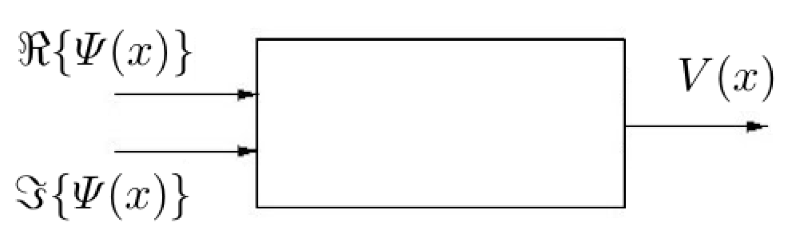
Assuming that the potential vanishes at some distance, after discretization and some manipulation with the indices, the integral equation in Equation (19) can be rewritten in the form of a system of linear equations, which can be solved with standard techniques. Here, however, the inverse problem is the topic of interest, which is very complicated to solve. In this case, the scattered wave function is used as the input, and the potential is the output of the system. The block structure of the inverse system can be seen in Figure 9, where the real and imaginary parts of the scattered wave $\mathsf{\Psi }\left(x\right)$ are used as input variables, and the $V\left(x\right)$ potential is the output variable of the system. However, it is worth noting that in real-life scattering experiments, the measured quantities are the transmission coefficients, phase-shifts, scattering cross-sections, etc., which usually depend on the asymptotic behavior of the wave functions. Although there are several possibilities to simplify the problem (e.g., Born approximation, WKB approximation), here, we assume that the scattered wave function is known everywhere (if this is not the case, it is still possible to estimate the potential with using the momentum-dependent phase shifts as inputs and the Fourier transform of the potential as the output, which could be a good method to analyze real-life data).

In this analysis, the wave number of the incoming wave is fixed at $k=0.5$ MeV, while the potential can vary between $V\in [-2,0]$ MeV, which will be the operating range of the identified system. Furthermore, the system is constructed so that the potential vanishes if $\left|x\right|>2$ MeV${}^{-1}$. In this way, the Lippmann–Schwinger equation can be solved numerically, and its solutions can be used as training data to identify the inverse system. One solution of the discretized Lippman–Schwinger equation with the mentioned constraints can be seen in Figure 10, where on the upper side there is a generated potential, while on the bottom side there is the output wave function with its real and imaginary parts shown. To identify the inverse system, only the red dotted part of the potential is used; however, this also means that near $\pm 2$ MeV${}^{-1}$, the wave function above or below $\pm 2$ MeV${}^{-1}$ has to be used because of the finite memory of the system. For this reason, the system is solved between $x\in [-3,3]$ MeV${}^{-1}$ where for the output $V\left(x\right)$, only the values between $-2$ MeV${}^{-1}$$\le x\le$ 2 MeV${}^{-1}$ are used, while for the input variables, the values up to $\left|x\right|\le M\mathsf{\Delta }x$ can be used as well if the memory (M) of the system requires it.

It is also possible to construct different kind of systems; for example, a system with a broader x and potential that approaches zero continuously at some distance; however, to further demonstrate the capabilities of the Volterra model, the system that was described previously is sufficient.

The identification of the system, which describes the inverse scattering problem, was shown in the previous section. Random potential functions are generated between $x\in [-2,2]$ MeV${}^{-1}$, which was discretized to get 80 points between this interval. After discretization, the Lippmann–Schwinger equation is solved on a larger $x\in [-3,3]$ MeV${}^{-1}$ interval, where the potential is considered zero if $\left|x\right|>2$, to achieve the training data. From each generated sample (from each solution), only one point and the values corresponding to the system memory are used as training data.

As it was shown in the previous section, the Volterra kernels could be estimated in the least squares sense by constructing a coefficient matrix $\mathit{X}$ from the input variables; then, we multiply the output with the pseudo-inverse of $\mathit{X}$. In the bound state problem, only one input was x-dependent, while here, both inputs depend on x; hence, the coefficient matrix and the corresponding $\mathit{H}$ vector have to be adjusted accordingly. Following Equation (11), the two input vectors ${\mathsf{\Psi }}_j^{\Re }\left(x_i\right)$ and ${\mathsf{\Psi }}_j^{\Im }\left(x_i\right)$ can be constructed for the real and imaginary parts of the wave functions, where j represents the order ($j=1\dots L$) and $x_i$ is the space point in the i’th sample. Due to the x-dependence in both of the inputs, the cross-terms will also differ from the previous example. For the simplest case, where both inputs are on the first order, it looks like:

$$\begin{array}{cc}\hfill & {\mathit{C}}^{1,1}\left(x_i\right)=[\Re \left\{\mathsf{\Psi }(x_i-M\mathsf{\Delta }x)\right\}\Im \left\{\mathsf{\Psi }(x_i-M\mathsf{\Delta }x)\right\},\dots ,\Re \left\{\mathsf{\Psi }(x_i-M\mathsf{\Delta }x)\right\}\Im \left\{\mathsf{\Psi }(x_i+M\mathsf{\Delta }x)\right\}\hfill \\ \hfill & \Re \left\{\mathsf{\Psi }(x_i-(M-1)\mathsf{\Delta }x)\right\}\Im \left\{\mathsf{\Psi }(x_i-M\mathsf{\Delta }x)\right\},\dots ,\Re \left\{\mathsf{\Psi }(x_i-(M-1)\mathsf{\Delta }x)\right\}\Im \left\{\mathsf{\Psi }(x_i+M\mathsf{\Delta }x)\right\}\hfill \\ \hfill & \dots ,\Re \left\{\mathsf{\Psi }(x_i+M\mathsf{\Delta }x)\right\}\Im \left\{\mathsf{\Psi }(x_i+M\mathsf{\Delta }x)\right\}],\hfill \end{array}$$

(21)

where for simplicity, it is assumed that both $\Re \left\{\mathsf{\Psi }\right(x\left)\right\}$ and $\Im \left\{\mathsf{\Psi }\right(x\left)\right\}$ have the same memory M. In the cross-terms, all the possible combinations of the real and imaginary parts have to be included, which is indicated by the first term in the second line in Equation (21). The higher order terms can be constructed the same way as the first order terms by taking all the possible combinations of the two inputs, which can have different orders. In this example, the memory of both inputs are fixed to the same value, and the coefficient matrix looks like:

$$\mathit{X}=\left[\begin{array}{cccccccccc}\hfill 1& \hfill {\mathsf{\Psi }}_1^{\Re }\left(x_1\right)& \hfill \dots & {\mathsf{\Psi }}_R^{\Re }\left(x_1\right)& {\mathsf{\Psi }}_1^{\Im }\left(x_1\right)& \dots & {\mathsf{\Psi }}_L^{\Im }\left(x_1\right)& {\mathit{C}}^{1,1}\left(x_1\right)& \dots & {\mathit{C}}^{R,L}\left(x_1\right)\\ \hfill 1& \hfill {\mathsf{\Psi }}_1^{\Re }\left(x_2\right)& \hfill \dots & {\mathsf{\Psi }}_R^{\Re }\left(x_2\right)& {\mathsf{\Psi }}_1^{\Im }\left(x_2\right)& \dots & {\mathsf{\Psi }}_L^{\Im }\left(x_2\right)& {\mathit{C}}^{1,1}\left(x_2\right)& \dots & {\mathit{C}}^{R,L}\left(x_2\right)\\ & & & \dots & \dots & \dots & \dots & & & \\ \hfill 1& \hfill {\mathsf{\Psi }}_1^{\Re }\left(x_{N_S}\right)& \hfill \dots & {\mathsf{\Psi }}_R^{\Re }\left(x_{N_S}\right)& {\mathsf{\Psi }}_1^{\Im }\left(x_{N_S}\right)& \dots & {\mathsf{\Psi }}_L^{\Im }\left(x_{N_S}\right)& {\mathit{C}}^{1,1}\left(x_{N_S}\right)& \dots & {\mathit{C}}^{R,L}\left(x_{N_S}\right)\end{array}\right]$$

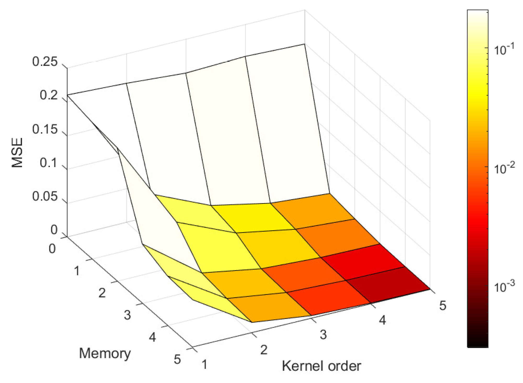
From the coefficient matrix, it is straightforward to construct the parameter vector $\mathit{H}$, which now consists of the parameters for the two x-dependent inputs and the new cross-terms as well. After the training data are generated, the coefficient matrix and the parameter and output vectors are constructed; the parameter identification goes as it was described in the previous section. In Figure 11, the mean squared error dependence on the memory and order of the system is shown when the cross-terms are neglected. On the upper figure, it can be seen that the MSE has a decreasing tendency when more memory is added to the system and/or the system has higher order kernels. On the bottom figure, the MSE dependence on the memory of the system is examined when the order of the system is kept at the same value. From this figure, it can be deduced that there is a limit to what can be achieved by only adding more and more memories to the system, as for each order the MSE will decrease, but the rate of this decline will slow down eventually. In conclusion, the higher order terms are necessary to describe the inverse scattering problem so the system is nonlinear in essence.

So far, the cross-terms are completely unable to simply show the memory and system order dependence of the mean squared error. In Figure 12, the kernel order dependence of the MSE is shown for a system with memory $M=5$ with and without the first cross-term $H_1\{\Re \left\{\mathsf{\Psi }\left(x\right)\right\},\Im \left\{\mathsf{\Psi }\left(x\right)\right\}\}$, where the notation $H_1\{\Re \left\{\mathsf{\Psi }\left(x\right)\right\},\Im \left\{\mathsf{\Psi }\left(x\right)\right\}\}$ corresponds to the ${\mathit{C}}^{1,1}\left(x_i\right)$ vector in Equation (21). It can be seen that the cross-terms indeed play a huge role in the description of the problem, as the MSE will be significantly lower in each order if the first cross-term is included. The 2nd, 3rd, and higher order cross-terms were not included in the examination, as the first order cross-term was sufficient to describe the system within a few percent accuracy.

In Figure 13, two examples are shown, where the identified system was a fourth order Volterra model, with $M=5$ memories, including the first order cross kernel $H_1\{\Re \left\{\mathsf{\Psi }\left(x\right)\right\},\Im \left\{\mathsf{\Psi }\left(x\right)\right\}\}$. In both cases, a really good match is achieved. Adding more terms could improve the model, as it was seen in Figure 11, where the errors tend to get smaller with the inclusion of higher order terms.

5. Stability of the Inverse System and the Effects of Input Noise

In this section, the stability of the inverted system is addressed, which is an important aspect of any numerical method, especially in real-life situations, where the input and/or output data have some additional noise. A well-posed problem requires that a unique solution exists, which continuously changes with the variation of the initial conditions of the system. Inverse problems are often ill-posed and are highly sensitive to the changes in the data. In the system identification sense, the stability of a dynamical system means that the output does not have large changes when there are small changes in its input. In linear system theory, there are well-developed techniques, which can be used to describe the different stability criteria, e.g., marginal stability or asymptotic stability; however, for nonlinear systems, it is much harder to prove such conditions. The stability of a system could be improved with regularization techniques, which are often used in real-life measurements, where measurement noise disturbs the data.

In this paper, only the underlying, noiseless, nonlinear systems were used in the identification of the Volterra kernels, and neither regularization nor an additional noise model were taken into account to impose extra conditions, e.g., smoothness. In this sense, the Volterra model is only able to describe the original dynamical system in a specified operation range given by the training data; hence, the sensitivity of the identified Volterra system is only as good as it is in the original dynamical system. To investigate the behavior of the Volterra model to additional disturbances, firstly, the identifiable nonlinear system is investigated, whose structure is shown in Figure 3 and is described by the Schrödinger equation. In this system, the inputs are the wave function $\mathsf{\Psi }\left(x\right)$ and the energy eigenvalue E, while the output is the potential function $V\left(x\right)$. To see the behavior of the system to additional disturbances, let us add the noise terms $n_{\mathsf{\Psi }}\left(x\right)$ and $n_E$ to the inputs $\mathsf{\Psi }\left(x\right)$ and E. Furthermore, let us assume that the x-dependent $n_{\mathsf{\Psi }}\left(x\right)$ disturbance is described by a continuous random process, which is uncorrelated with the input $\mathsf{\Psi }\left(x\right)$. After rearranging the terms in the original Schrödinger equation and adding the extra noise terms, the corresponding input–output relation will be:

$$\frac{1}{2m(\mathsf{\Psi }\left(x\right)+n_{\mathsf{\Psi }}\left(x\right))}\frac{d^2(\mathsf{\Psi }\left(x\right)+n_{\mathsf{\Psi }}\left(x\right))}{d{x}^2}+(E+n_E)=V\left(x\right)+\mathsf{\Delta }V\left(x\right),$$

(22)

where $n_{\mathsf{\Psi }}\left(x\right)$ and $n_E$ are the additional noises on the wave function and the energy eigenvalues, respectively, while $\mathsf{\Delta }V\left(x\right)$ is the corresponding change in the potential function due to the disturbances on the input variables. Assuming that the disturbances are small, e.g., $|n_{\mathsf{\Psi }}\left(x\right)|\ll |\mathsf{\Psi }\left(x\right)|$ for every x, the term in the denominator can be approximated by $\mathsf{\Psi }\left(x\right)+n_{\mathsf{\Psi }}\left(x\right)\approx \mathsf{\Psi }\left(x\right)$, and the output difference $\mathsf{\Delta }V\left(x\right)$ can be expressed as:

$$\mathsf{\Delta }V\left(x\right)\approx \frac{1}{2m\mathsf{\Psi }\left(x\right)}\frac{d^2{n}_{\mathsf{\Psi }}\left(x\right)}{d{x}^2}+n_E,$$

(23)

where it can be seen that the most problematic part is the second derivative of $n_{\mathsf{\Psi }}\left(x\right)$, because even if $|n_{\mathsf{\Psi }}\left(x\right)|\ll |\mathsf{\Psi }\left(x\right)|$ is satisfied for every x, the second derivative of $n_{\mathsf{\Psi }}\left(x\right)$ could still be much larger than the second derivative of the noiseless wave function; therefore, the error in $\mathsf{\Psi }\left(x\right)$ could give a dominant contribution to the measured output. In contrast, the error in the energy does not give a dominant contribution to $\mathsf{\Delta }V$ if $|n_E|\ll |E|$.

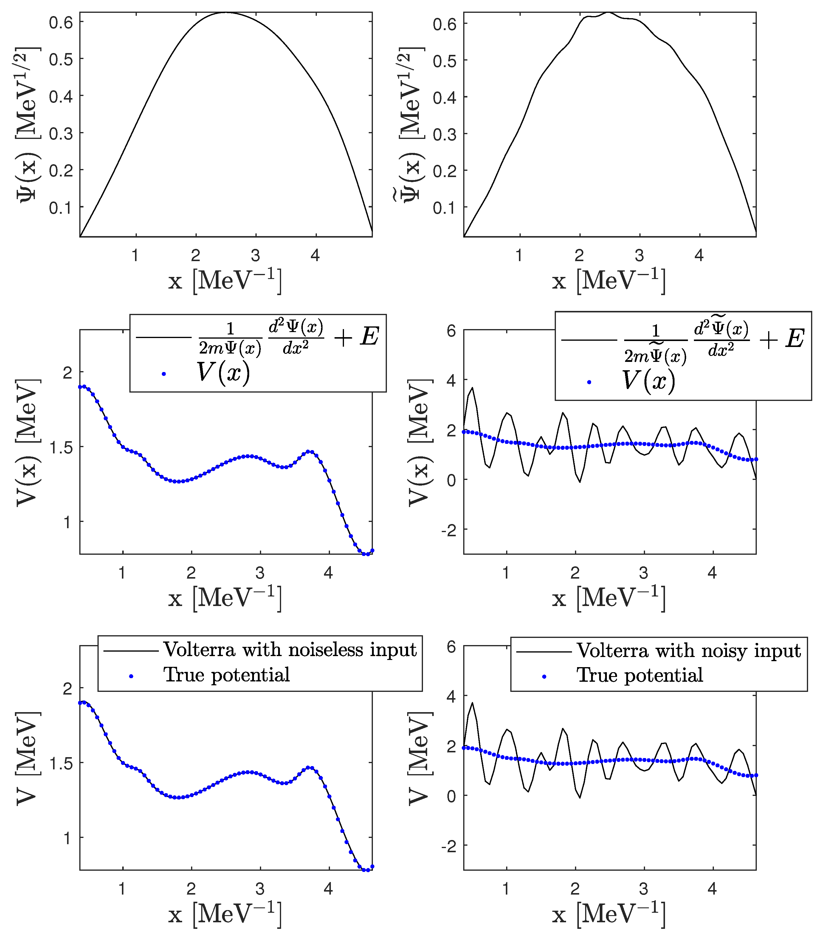
To see the effects of the mentioned behavior, a simple error calculation is made to the bound state problem described in Section 3 for a randomly generated potential and the corresponding bound state wave function and energy eigenvalue. The input noise of the wave function $n_{\mathsf{\Psi }}\left(x\right)$ is assumed to be a band-limited Gaussian noise, with zero mean and a standard deviation, which is 1–2% of the input $u\left(x_i\right)$ variables. The bandwidth is set to be $0.3$ times the Nyquist rate, to suppress the high-frequency parts of the noise function. Due to its little effect on the output, and to simplify the calculations, the error of the energy $n_E$ is neglected from now on. The results can be seen in Figure 14, where it can be seen that the original dynamical model is quite sensitive to the input noise, which is the expected behavior. From the bottom two figures, which show the results of the identified Volterra system, with and without noise, it can be seen that the identified model shows the same behavior as the original system. This is also expected as the identification has been done to noiseless input and output data. It is also reassuring that the Volterra model does not break down to the inclusion of previously unknown additional noise, which was not present at the identification stage.

It is also interesting to check how the output noise (generated by the input noise) behaves regarding averaging. Generally, in system identification, the noise has to be modeled, e.g., with parametric or non-parametric noise models [65], and in addition, extra care should be taken when the noise is correlated, which is usually the case in real measurements. If the correlation is small, and the noise is Gaussian, the simple weighted average is still a robust estimator independent of the details of the correlation; however, it is in exchange for a non-optimal error for the average [66]. The Volterra representation estimates the true model with a combination of products of the input variables, which all have additive noise terms; therefore, it is not that straightforward to analyze the propagated errors and its correlations. In real experiments, this has to be addressed thoroughly; however, here, only an estimation will be given. It can been seen from Equation (23) that in the true model, the dominant error comes from the second derivative of the input errors; therefore, at least in the original model, the input-filtered Gaussian noise will (at least approximately) stay as a Gaussian with the same zero mean and with some other variance. Let us assume that the Volterra model estimates this behavior; therefore, through averaging the model output, one could obtain the true potential. To see this, a simple calculation is made with the identified Volterra model, where the number of samples used for averaging is set to be $N_{sample}=10,100,1000$, and 5000, respectively. The results are shown in Figure 15, where it can be seen that the uncertainty of the output is getting smaller with the increasing number of samples.

6. Conclusions

In this paper, a non-causal Volterra model representation is used to describe the inverse problem in quantum mechanics, where an unknown potential has to be found from the information carried by the wave functions. The Volterra model is capable of describing nonlinear dynamical systems and can be used in many applications in engineering. Here, it is used to describe quantum mechanical inverse problems, whose solutions are not straightforward. The non-causal description, where an output at x depends not just on the previous but also the future values of the input, seems to be necessary to describe the inverse problems in quantum mechanics. To show the model capabilities, two simple examples were given. First, the quantum mechanical bound state problem is addressed, where using the wave function and its corresponding energy eigenvalue, the potential in a box could be estimated through a 5th order Volterra model with a finite memory. In this example, there was no need for cross-terms in the Volterra representation, as the energy eigenvalue only acts as a shift in the inverse problem. The second example is a simplified one-dimensional quantum scattering problem, where a particle, described by a free wave function, is scattered on some bounded potential, giving a scattered wave. In the inverse problem, the real and imaginary parts of the scattered wave functions are used as inputs of the system, while the potential acts as the output. For this problem, a 4th order Volterra system is identified, where it seemed to be necessary to include at least the first order cross-term to be able to give satisfactory results. In both examples, higher order terms were necessary to describe the inverse problems, which indicates that they are nonlinear in nature. The stability of the Volterra model has been investigated using the bound state problem, where it has been observed that even with additional input noise, the Volterra representation is able to reproduce the potentials through averaging the model output.

The non-causal Volterra model described here is very general and can be used in many problems from engineering to quantum mechanics. Its main advantage is that it is capable of describing nonlinear dynamical systems with static or dynamic nonlinearities, which often arise in inverse problems. The disadvantage of the Volterra representation is the numerical complexity of the kernel estimation for complex systems, where the memory could be large. One of the possible applications of the model could be the determination of potentials in scattering experiments, where even if the underlying dynamics are well known, the experimental setup could bring in extra nonlinearities in the system, which has to be modeled. Simplified nonlinear dynamical models could also be identified by this method through experiments, which is also a great advantage of the Volterra method. For future applications, the model will be extended to describe real-life scattering data, where the measured phase-shifts and differential cross-sections will be used as input variables.

References

- Ogawa, T.; Kanada, H. Solution for Ill-Posed Inverse Kinematics of Robot Arm by Network Inversion. J. Robot. 2010, 2010, 870923. [Google Scholar] [CrossRef] [Green Version]
- Craig, J.J. Introduction to Robotics: Mechanics and Control; Addison-Wesley: Reading, MA, USA, 1986. [Google Scholar]
- Jaluria, Y. Solution of Inverse Problems in Thermal Systems. J. Therm. Sci. Eng. Appl. 2019, 12, 011005. [Google Scholar] [CrossRef]
- Gelin, J.C.; Ghouati, O. An inverse method for material parameters estimation in the inelastic range. Comp. Mech. 1995, 16, 143–150. [Google Scholar] [CrossRef]
- Mackintosh, R.S.; Cooper, S.G. Using inverse scattering methods to study inter-nucleus potentials. J. Phys. G Nucl. Part. Phys. 1998, 24, 1599–1610. [Google Scholar] [CrossRef]
- Mackintosh, R.; Cooper, S. Exchange contributions to nucleus-nucleus potentials deduced from RGM phase shifts using inversion. Nucl. Phys. A 1995, 589, 377–394. [Google Scholar] [CrossRef]
- Kukulin, V.I.; Mackintosh, R.S. The application of inversion to nuclear scattering. J. Phys. G Nucl. Part. Phys. 2004, 30, R1–R55. [Google Scholar] [CrossRef]
- Lipperheide, R.; Fiedeldey, H. Inverse problem for potential scattering at fixed energy. Z. Phys. A 1978, 286, 45–56. [Google Scholar] [CrossRef]
- Egorova, I.; Gladka, Z.; Lange, T.; Teschl, G. Inverse Scattering Theory for Schrödinger Operators with Steplike Potentials. Zhurnal Mat. Fiz. Anal. Geom. 2015, 11, 123–158. [Google Scholar] [CrossRef] [Green Version]
- Kay, I.; Moses, H. The determination of the scattering potential from the spectral measure function. Il Nuovo Cimento 1961, 22, 689–705. [Google Scholar] [CrossRef]
- Yagle, A.E. Discrete Gel’fand-Levitan and Marchenko matrix equations and layer stripping algorithms for the discrete two-dimensional Schrödinger equation inverse scattering problem with a nonlocal potential. Inverse Probl. 1998, 14, 763–778. [Google Scholar] [CrossRef] [Green Version]
- Bruckstein, A.M.; Levy, B.C.; Kailath, T. Differential methods in inverse scattering. SIAM J. Appl. Math. 1985, 45, 312–335. [Google Scholar] [CrossRef]
- Chadan, K.; Sabatier, P.C. Inverse Problems in Quantum Scattering Theory; Springer: Berlin/Heidelberg, Germany, 1989. [Google Scholar]
- Faddeyev, L.D.; Seckler, B. The Inverse Problem in the Quantum Theory of Scattering. J. Math. Phys. 1963, 4, 72–103. [Google Scholar] [CrossRef]
- Newton, R.G. Inversion of reflection data for layered media: A review of exact methods. Geophys. J. Int. 1981, 65, 191–215. [Google Scholar] [CrossRef] [Green Version]
- Ljung, L. Perspectives on system identification. Ann. Rev. Contr. 2010, 34, 1–12. [Google Scholar] [CrossRef] [Green Version]
- Palm, G.; Poggio, T. The Volterra Representation and the Wiener Expansion: Validity and Pitfalls. J. Appl. Math. 1977, 33, 195–216. [Google Scholar] [CrossRef]
- Cheng, C.; Peng, Z.; Zhang, W.; Meng, G. Volterra-series-based nonlinear system modeling and its engineering applications: A state-of-the-art review. MSSP 2017, 87, 340–364. [Google Scholar] [CrossRef]
- Palm, G.; Pöpel, B. Volterra representation and Wiener-like identification of nonlinear systems: Scope and limitations. Quart. Rev. Biophys. 1985, 18, 135–164. [Google Scholar] [CrossRef]
- Tan, L.; Jiang, J. Digital Signal Processing: Fundamentals and Applications; Elsevier: Amsterdam, The Netherlands, 2018. [Google Scholar]
- Stegmayer, G.; Pirola, M.; Orengo, G.; Chiotti, O. Towards a Volterra series representation from a Neural Network model. WSEAS Trans. Syst. 2004, 3, 432–437. [Google Scholar]
- Korenberg, M.J.; Hunter, I.W. The identification of nonlinear biological systems: Volterra kernel approaches. Ann. Biomed. Eng. 2007, 24, 250–268. [Google Scholar] [CrossRef]
- Paula, N.C.G.; Marques, F.D.; Silva, W.A. Volterra Kernels Assessment via Time-Delay Neural Networks for Nonlinear Unsteady Aerodynamic Loading Identification. AIAA J. 2018, 57, 1–11. [Google Scholar]
- Balajewicz, M.; Nitzsche, F.; Feszty, D. Application of Multi-Input Volterra Theory to Nonlinear Multi-Degree-of-Freedom Aerodynamic Systems. AIAA J. 2010, 48, 56–62. [Google Scholar] [CrossRef]
- Kamyad, A.V.; Mehne, H.H.; Borzabadi, A.H. The Best Linear Approximation for Nonlinear Systems. Appl. Math. Comp. 2005, 167, 1041–1061. [Google Scholar] [CrossRef]
- Fréchet, M. Sur les fonctionnelles continues. Ann. L’Ecole Norm. Supér. 1910, 27, 193–216. [Google Scholar] [CrossRef] [Green Version]
- Boyd, S.; Chua, L.O. Analytical Foundations of Volterra Series. IMA J. Math. Contrl. Inf. 1984, 1, 243–282. [Google Scholar] [CrossRef]
- Sidorov, D. Integral Dynamical Models: Singularities, Signals and Control; World Scientific Series on Nonlinear Science Series A; World Scientific: Singapore, 2014; Volume 87. [Google Scholar]
- Sidorov, D.N.; Sidorov, N.A. Generalized solutions in the problem of dynamical systems modeling by Volterra polynomials. Autom. Remote Control 2011, 72, 1258–1263. [Google Scholar] [CrossRef]
- Meshkov, S.I. Stationary mode of a nonlinear elastically hereditary oscillator. J. Appl. Mech. Tech. Phys. 1970, 11, 458–462. [Google Scholar] [CrossRef]
- Franklin, G.F.; Powell, J.D.; Emami-Naeini, A. Feedback Control of Dynamic Systems, 7th ed.; Pearson: Stanford, CA, USA, 2014. [Google Scholar]
- Aliyev, T.; Gatzke, E. Prioritized constraint handling NMPC using Volterra series models. Optim. Control Appl. Methods 2010, 31, 415–432. [Google Scholar] [CrossRef]
- Yoon, Y.; Sun, Z. Robust Motion Control for Tracking Time-Varying Reference Signals and Its Application to a Camless Engine Valve Actuator. IEEE Trans. Ind. Electron. 2016, 63, 5724–5732. [Google Scholar] [CrossRef]
- Belbas, S.A.; Bulka, Y. Numerical Solution of Multiple Nonlinear Volterra Integral Equations. Appl. Math. Comput. 2011, 217, 4791–4804. [Google Scholar] [CrossRef] [Green Version]
- Sidorov, D.; Sidorov, N. Numerical Solution of Multiple Nonlinear Volterra Integral Equations. Banach J. Math. Anal. 2012, 6, 1–10. [Google Scholar] [CrossRef]
- Thomas, E.G.F.; van Hemmen, J.L.; Kistler, W.M. Calculation of Volterra kernels for solutions of nonlinear differential equations. J. Appl. Math. 2006, 61, 1–21. [Google Scholar] [CrossRef] [Green Version]
- Stepniak, G.; Kowalczyk, M.; Siuzdak, J. Volterra Kernel Estimation of White Light LEDs in the Time Domain. Sensors 2018, 18, 1024. [Google Scholar] [CrossRef] [PubMed] [Green Version]
- Sarkas, I.; Mavridis, D.; Papamichail, M.; Papadopoulos, G. Volterra Analysis Using Chebyshev Series. Proc. IEEE Int. Symp. Circ. Syst. 2007, 1931–1934. [Google Scholar] [CrossRef]
- Sarkas, I.; Mavridis, D.; Papamichail, M. Large and small signal distortion analysis using modified Volterra series. Analog Integr. Circ. Sig. Process 2008, 54, 133–142. [Google Scholar] [CrossRef]
- Zhang, B.; Billings, S. Volterra series truncation and kernel estimation of nonlinear systems in the frequency domain. Mech. Syst. Sign. Proc. 2017, 84, 39–57. [Google Scholar] [CrossRef]
- Marmarelis, V.; Zhao, X. Volterra models and three-layer perceptrons. IEEE Trans. Neural Netw. 1997, 8, 1421–1433. [Google Scholar] [CrossRef] [Green Version]
- Zhong, K.; Chen, L. An Intelligent Calculation Method of Volterra Time-Domain Kernel Based on Time-Delay Artificial Neural Network. Math. Prob. Eng. 2020, 2020, 1–11. [Google Scholar] [CrossRef]
- Wray, J.; Green, G. Calculation of the Volterra kernels of non-linear dynamic systems using an artificial neural network. Biol. Cybern. 1994, 71, 187–195. [Google Scholar] [CrossRef]
- Waibel, A.; Hanazawa, T.; Hinton, G.; Shikano, K.; Lang, K. Phoneme recognition using time-delay neural networks. IEEE Trans. Acoust. Speech Signal Process. 1989, 37, 328–339. [Google Scholar] [CrossRef]
- Apartsyn, A.S. Nonclassical Linear Volterra Equations of the First Kind; Walter de Gruyter: Berlin, Germany, 2003. [Google Scholar]
- Hélie, T.; Hasler, M. Volterra series for solving weakly non-linear partial differential equations: Application to a dissipative Burgers equation. Int. J. Control 2004, 77, 1071–1082. [Google Scholar] [CrossRef]
- Simos, T.; Williams, P. A finite-difference method for the numerical solution of the Schrödinger equation. J. Comput. Appl. Math. 1997, 79, 189–205. [Google Scholar] [CrossRef] [Green Version]
- Mowlavi, A.A.; Arabshahi, H. Application of Runge-Kutta Numerical Methods to Solve the Schrodinger Equation for Hydrogen and Positronium Atoms. Res. J. Appl. Sci. 2010, 5, 315–319. [Google Scholar] [CrossRef] [Green Version]
- Mitchell, T. Machine Learning; McGraw Hill: New York, NY, USA, 1997. [Google Scholar]
- Franz, M.O.; Schölkopf, B. A Unifying View of Wiener and Volterra Theory and Polynomial Kernel Regression. Neural Comput. 2006, 18, 3097–3118. [Google Scholar] [CrossRef] [PubMed]
- Smola, A.J.; Schölkopf, B. A tutorial on support vector regression. Stat. Comput. 2004, 14, 199–222. [Google Scholar] [CrossRef] [Green Version]
- Griffiths, D.J.; Schroeter, D.F. Introduction to Quantum Mechanics, 3rd ed.; Cambridge University Press: Cambridge, UK, 2018. [Google Scholar]
- Landsman, N.P. Born Rule and Its Interpretation; Springer: Berlin/Heidelberg, Germany, 2009; pp. 64–70. [Google Scholar]
- Bohm, A.R.; Uncu, H.; Komy, S.R. A brief survey of the mathematics of quantum physics. Rep. Math. Phys. 2009, 64, 5–32. [Google Scholar] [CrossRef]
- Mihály, L.; Martin, M.C. Solid State Physics: Problems and Solutions, 2nd ed.; John Wiley & Sons: Hoboken, NJ, USA, 2009. [Google Scholar]
- Lim, Y.K. Problems and Solutions on Atomic, Nuclear and Particle Physics; World Scientific Publishing: Singapore, 2000. [Google Scholar]
- Killingbeck, J. Shooting methods for the Schrödinger equation. J. Phys. A Math. Gen. 1987, 20, 1411–1417. [Google Scholar] [CrossRef]
- Lesiak, C.; Krener, A. The existence and uniqueness of Volterra series for nonlinear systems. IEEE Trans. Autom. Control 1978, 23, 1090–1095. [Google Scholar] [CrossRef]
- Golub, G.; Loan, C. Orthogonalization and Least squares. In Matrix Computations, 3rd ed.; University Press: Baltimore, MD, USA, 1996. [Google Scholar]
- Skyvulstad, H.; Petersen, Ø.W.; Argentini, T.; Zasso, A.; Øiseth, O. The use of a Laguerrian expansion basis as Volterra kernels for the efficient modeling of nonlinear self-excited forces on bridge decks. J. Wind Eng. Ind. Aerodyn. 2021, 219, 104805. [Google Scholar] [CrossRef]
- Lambert, J.D. Numerical Methods for Ordinary Differential Systems: The Initial Value Problem; John Wiley & Sons, Inc.: Hoboken, NJ, USA, 1991. [Google Scholar]
- Viterbo, V.; Lemes, N.; Braga, J. Variable phase equation in quantum scattering. Rev. Bras. Ensino Física 2014, 36, 1–5. [Google Scholar] [CrossRef] [Green Version]
- Baym, G. Lectures on Quantum Mechanics; W. A. Benjamin, Inc.: Reading, MA, USA, 1969. [Google Scholar]
- Barlette, V.E.; Leite, M.M.; Adhikari, S.K. Integral equations of scattering in one dimension. Am. J. Phys. 2001, 69, 1010–1013. [Google Scholar] [CrossRef] [Green Version]
- Schoukens, J.; Pintelon, R.; Rolain, Y. Mastering System Identification in 100 Exercises; John Wiley & Sons: Hoboken, NJ, USA, 2012. [Google Scholar]
- Schmelling, M. Averaging correlated data. Phys. Scr. 1995, 51, 676–679. [Google Scholar] [CrossRef]
Figure 1.
Block diagrams of the possible systems, where the MIMO and MISO systems contain only two inputs and .
Figure 2.
Sketch of the quantum mechanical bound state problem, where a particle is constrained in a finite sized box, with a potential inside.
Figure 3.
Identifiable system for the quantum mechanical bound state problem in one dimension. On the left side, the underlying dynamical system is shown, while on the right side, the simplified sketch of the MISO system in question is shown, where is the normalized wave function and is the energy of the first bound state.
Figure 4.
One generated random potential and its corresponding bound sate, which is used to identify the Volterra kernels. From every sample, one randomly generated point (red circle) is chosen for the training data. If the memory of the Volterra system is , the corresponding neighboring points are also used, which is indicated by red crosses on the bottom figure.
Figure 5.
Mean squared error dependence on the memory and order of the Volterra representation of the inverse system.
Figure 6.
MSE dependence on the order of the input, where some cross-terms are also included. The error after the linear order is not decreasing, which indicates that the system only depends on linearly.
Figure 7.
Comparison of the training data with the output of the identified 5th order Volterra system. The black lines are the training samples, while the blue dotted lines are the model outputs.
Figure 8.
Comparison of the true potential and the calculated potential from the Volterra model in two different cases. The black lines are the true potentials, while the blue dotted lines are the model calculations given by the identified 5th order Volterra system.
Figure 9.
Identifiable system for the inverse quantum scattering problem. The two inputs are the real and imaginary parts of the scattered wave function, while the output is the scattering potential.
Figure 10.
Solution of the Lippmann–Schwinger equation for the potential function shown in the upper figure for an initial wave function , with MeV. The part of the potential marked by red dots are the values, which are used as outputs of the system. The lower figure shows the imaginary and real values of the scattered wave function, which are used as inputs of the Volterra system.
Figure 11.
Mean squared error dependence on the memory and on the order of the Volterra system without cross-terms. On the bottom figure, the MSE dependence on the memory is shown at fixed kernel orders.
Figure 12.
The mean squared error dependence on the kernel order with and without the first cross-term in the Volterra representation, when the memory is fixed to .
Figure 13.
Comparison of the true potential and the estimated potential for two different configurations, calculated by the identified 4th order Volterra model, including the first-order cross kernel , with memories.
Figure 14.
Output sensitivity test for the inverse bound state problem, with an additive band-limited Gaussian noise on the input wave function . The left side shows a noiseless case, while the three figures in the right column show the noisy results. The upper two figures show the noiseless and noisy input wave functions, the middle two figures show the results of the true dynamical model, while the bottom two figures show the results obtained by the Volterra model for the noiseless and for the noisy case, respectively.
Figure 15.
Averaging the output of the identified Volterra model to noisy inputs. The black lines are the outputs of the Volterra model, while the blue dots are the true potentials that correspond to the noiseless inputs.
Publisher’s Note: MDPI stays neutral with regard to jurisdictional claims in published maps and institutional affiliations. |
© 2022 by the author. Licensee MDPI, Basel, Switzerland. This article is an open access article distributed under the terms and conditions of the Creative Commons Attribution (CC BY) license (https://creativecommons.org/licenses/by/4.0/).
Share and Cite
MDPI and ACS Style
Balassa, G. Estimating Scattering Potentials in Inverse Problems with a Non-Causal Volterra Model. Mathematics 2022, 10, 1257. https://doi.org/10.3390/math10081257
AMA Style
Balassa G. Estimating Scattering Potentials in Inverse Problems with a Non-Causal Volterra Model. Mathematics. 2022; 10(8):1257. https://doi.org/10.3390/math10081257
Chicago/Turabian StyleBalassa, Gábor. 2022. "Estimating Scattering Potentials in Inverse Problems with a Non-Causal Volterra Model" Mathematics 10, no. 8: 1257. https://doi.org/10.3390/math10081257
Note that from the first issue of 2016, this journal uses article numbers instead of page numbers. See further details here.